Neural Disaggregation via Spatially Coherent Architectures

Abstract.

Open data is frequently released spatially and temporally aggregated, usually to comply with privacy policies. Varying aggregation levels (e.g., zip code, census tract, city block) complicate the integration across variables needed to provide multi-variate training sets for downstream AI/ML systems. In this work, we consider models to disaggregate spatial data, learning a function from a low-resolution irregular partition (e.g., zip code) to s high-resolution irregular partition (e.g., city block). We propose a hierarchical architecture that aligns each geographic aggregation level with a layer in the network such that all aggregation levels can be learned simultaneously by including loss terms for all intermediate levels as well as the final output. We then consider additional loss terms that compare the re-aggregated output against ground truth to further improve performance. To balance the tradeoff between training time and accuracy, we consider three training regimes, including a layer-by-layer process that achieves competitive predictions with significantly reduced training time. For situations where limited historical training data is available, we study transfer learning scenarios and show that a model pre-trained on one city variable can be fine-tuned for another city variable using only a few hundred samples, highlighting the common dynamics among variables from the same built environment and underlying population. Evaluating these techniques on four datasets across two cities, three variables, and two application domains, we find that geographically coherent architectures provide a significant improvement over baseline models as well as typical heuristic methods, advancing our long-term goal of synthesizing any variable, at any location, at any resolution.

1. Introduction

High-quality, longitudinal, and freely available urban data, coupled with advances in machine learning, improve our understanding and management of urban environments (Han and Howe, 2023). Over the last two decades, cities have increasingly released datasets publicly on the web, proactively, in response to transparency regulation. For example, in the US, all 50 states and the District of Columbia have passed some version of the federal Freedom of Information (FOI) Act. While this first wave of open data was driven by FOI laws and made national government data available primarily to journalists, lawyers, and activists, a second wave of open data, enabled by the advent of open source and web 2.0 technologies, was characterized by an attempt to make data “open by default” to civic technologists, government agencies, and corporations (Verhulst et al., 2020).

Open data affords study of urban dynamics (Vogel et al., 2011; Yu et al., 2017), but, with few exceptions (Zhang et al., 2020; Singh and Chen, 2023), models assume access to individual-level data, while privacy concerns motivate the release of aggregated data (Green et al., 2017) such that aggregated data tends to be the norm in some fields (Burrell et al., 2004; Lozano et al., 2009; Law et al., 2018). Although aggreggation can protect individual privacy (Ullah et al., 2021; Erkin et al., 2013; He et al., 2007) (without strong guarantees (Jia et al., 2022; Brauneck et al., 2023)), it complicates integration of multiple datasets (e.g., aligning tract-level to block-level data) and destroys information useful for training. For example, demographers have studied disaggregation techniques to uncover local hotspots erased by tract-level aggregation (Monteiro et al., 2018).

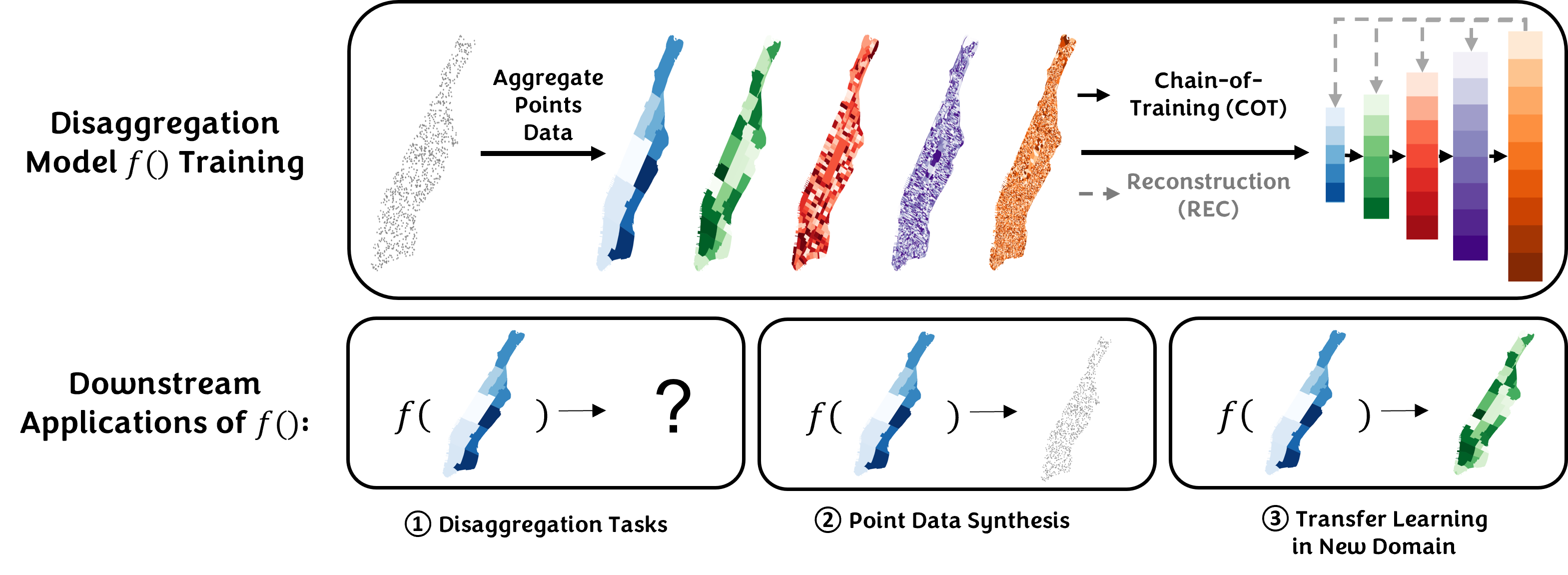
Figure 1. (Top) Individual events aggregated a multiple levels are used to train a model to disaggregate multiple levels simultaneously, with our proposed Chain-of-Training (COT) and Reconstruction (REC) strategy. (Bottom) These disaggregation functions can then be used in downstream applications to synthesize data, even for out-of-domain variables.

In this work, we consider learning techniques to synthesize higher-resolution urban data from lower-resolution aggregated urban data. We consider a set of spatiotemporal events (taxi pickups, 911 calls, tweets, etc.) that each occur within a given irregular polygonal region (census tract, zip code, city block, etc.) at a particular time. The disaggregation problem, then, is to learn a function from a coarse partitioning to a fine partitioning of the same domain that is predictive on unseen data. This function can be learned from historical event data when available, and in some cases can be learned from related variables. Figure 1 illustrates the setting.

Spatial disaggregation methods in the demography literature tend to rely on heuristics: areal weighting, which assumes all variables are constant per unit area (Comber and Zeng, 2019), and dasymetric mapping (Comber and Zeng, 2019), which assumes sufficient auxiliary data is available to predict the target variable using linear methods. Disaggregation has also been considered in the machine learning literature, outside of the spatiotemporal context, where the goal is to learn individual-level models given group-level aggregated data (Zhang et al., 2020; Monteiro et al., 2019a). However, these approaches explicitly seek a linear model where the target variable at the individual level is linearly determined only by the features at its group level as opposed to the interdependent features of other groups. In a spatiotemporal context, any region may influence any other: traffic on the bridge can increase wait times in midtown.

In this paper, we evaluate neural architectures for the disaggregation problem. Our overarching approach is to use a geographically coherent architecture, where certain layers in the network correspond to real aggregation levels. This approach introduces additional loss terms that penalize the model if the intermediate layers deviate from their real-world distributions. Intuitively, we encourage the model to “show its work” in computing the final output by ensuring that the intermediate results also agree with ground truth. The introduced loss terms, one for each level, are then weighted to account for the relative resolutions at each level. We refer to this strategy of using a spatially coherent architecture with area-weighted loss terms as Chain-of-Training (COT).

We then consider reconstruction (REC) error: the final output at high resolution can be re-aggregated to provide predictions at intermediate resolutions. These predictions can be compared with ground truth and included as additional loss terms to enforce self-consistency. We consider three strategies: a bridge strategy, where each level $i$ is used to reconstruct level $i-1$, a bottomup strategy, where the finest level is used to reconstruct all coarser levels, and a full strategy, where all possible reconstructions are included.

We also consider three training regimes for COT when the goal is to learn disaggregations to multiple levels: separate models for each target level, one overall model that produces estimates at all levels simultaneously, and a layer-by-layer training process where each aggregation level is trained then frozen before adding the next level and repeating the process. We find that the layer-by-layer regime significantly reduces training time and approximates the best results of training separate models for each level. We then show that a sampling scheme can be used to generate a realistic individual-level dataset of events that achieves high mutual information with the original data. Finally, we relax the assumption that longitudinal historical data is always available and consider pre-training on a variable A then fine-tuning on variable B.

Overall, we make the following contributions:

• We propose a spatially coherent architecture (COT) equipped with area-weighted loss terms to learn to disaggregate spatial data. Each layer corresponds to an aggregation level, affording a multi-task learning approach that allows all levels to be trained simultaneously. Together, these features deliver an 6.38% improvement over a baseline neural model and a 26.64% improvement over the best classical methods.

• We propose additional loss terms based on comparing reconstuctions with ground truth, encouraging self-consistency during training. Training strategies using these reconstruction terms improve performance an additional 1.15% for 2 out of 4 datasets.

• We consider both raster and vector representations of aggregated spatiotemporal data. We find that although raster representations better accommodate computer vision techniques (e.g., convolutional layers), the error introduced by converting into and out of raster formats are prohibitive.

• We propose and evaluate three training strategies for learning multiple disaggregations: separate training, joint training, and a layer-by-layer training approach. We find that the layer-by-layer approach significantly reduces training time while approximating the performance of training separate models.

• We show that individual-level datasets re-sampled from learned disaggregated regions are similar to the original dataset (via mutual information and Kullback–Leibler (KL) divergence.

• We consider a transfer learning setting, relaxing the assumption of longitudinal training data for every variable. We show the conditions under which parameters learned from one city variable can be used to make predictions from another.

• We evaluate proposed methods on four real datasets covering multiple experimental conditions: (same city, different variable); (same city, different application domain); (different city, same variable). These experiments show that proposed techniques can improve performance across all conditions.

2. Related Work

Spatial Disaggregation

Spatial disaggregation is frequently used in demography to infer individual records from spatially aggregated regions such as census data (Qiu et al., 2019; Wardropa et al., 2018), in applications including disease mapping (Arambepola et al., 2020) and vaccination coverage (Utazi et al., 2018). The area of spatial disaggregation is highly relevant to our study.

The common approach is areal weighting (AW), which assumes the value per unit area is constant (Goodchild et al., 1993). This method is common in practice due to its simplicity, general reliability, and ability to computed from a single variable. Pycnophylactic interpolation (PI), first introduced by Tobler in 1979 (Tobler, 1979), works similarly to areal weighting, but with a refinement to avoid discontinuties at the boundaries. PI distributes the values from source regions to target regions in an iterative manner, considering a weighted average of its nearest neighbors to avoid discontinuities while preserving the total count. Dasymetric mapping/interpolation/weighting (DM) approach is a family of methods that use the relationships between multiple variables to improve the estimated distribution. Unlike areal weighting scheme, dasymetric mapping uses auxiliary information to generate a weighted distribution of source values onto the target regions. Recent methods incorporate machine learning approaches to model the relationships between auxiliary data and source values and determine the weights for disaggregation (Qiu et al., 2019; Monteiro et al., 2018, 2019b). Sources of auxiliary information include satellite images (Stevens et al., 2015), 3D building information (Qiu et al., 2019), mobile phone usage data (Deville et al., 2014), terrain elevation and human settlement (Monteiro et al., 2019b), and other variables more broadly available at high spatial and temporal resolution. Despite the popularity of dasymetric mapping methods in spatial disaggregation, there are several potential limitations of them (Comber and Zeng, 2019). They are wholly dependent on auxiliary variables, which are not always available (e.g., remote sensing images or land type data in population disaggregation tasks). Additionally, the performance of the model depends on the quality of the auxiliary information and the relevance between the auxiliary data and source values.

Learning From Aggregated Observations

In addition to the spatial disaggregation methods, it is also possible to learn individual level probabilistic models from aggregated data, without direct decomposing aggregated data into individual instances. The problem is generally referred to as learning from aggregated observations, where supervision labels are given to sets of instances instead of individual instances, while the goal is still to make inferences on unseen individuals (Zhang et al., 2020; Singh and Chen, 2023; Law et al., 2018). Zhang et al. (Zhang et al., 2020) present a general probabilistic framework capable of accommodating a variety of aggregate observations for various tasks, such as classification and regression. They showed that simple maximum likelihood solutions can be applied to various differentiable models such as deep neural networks and gradient boosting machines. Ma et al. (Ma et al., 2020) studied the problem of learning nonlinear dynamics from aggregated data, where individual trajectory data is not available. They proposed a partial differential equation to describe the density evolution of aggregated data, which is subsequently combined with Wasserstein generative adversarial network (WGAN) in the training process. Wei et al. (Wei et al., 2023) studies a more specific problem — classification from aggregate observations (CFAO), where the supervision is provided to groups of instances, instead of individual instances. They presented a novel universal method of CFAO, which generates unbiased estimators of the classification risk for arbitrary losses.

Open Data Integration

Our motivation in this work is to improve the utility of open data for use in machine learning applications. Integration of open data through the discovery of join and union relationships shares this motivation. Miller proposed discovering queries that translate one dataset into another (Miller, 2018). Nargesian et al. (Nargesian et al., 2018) presented a probabilistic approach to identify tables within extensive repositories that can be effectively combined with a query table. They employed three statistical models that explain the generation of unionable attributes from three domains. Additionally, they proposed a data-driven approach that automatically determines the best model to use for each pair of attributes. Khatiwada et al. introduced ALITE (Khatiwada et al., 2022) to scalably integrate tables discovered through join, union, or related table search operations. ALITE relaxes schema assumptions around shared attributes, completeness, and acyclic join patterns and showed that ALITE outperforms previous algorithms for data integration via Full Disjunction. Khatiwada et al. (Khatiwada et al., 2023) proposed using semantic relationships between pairs of columns to enhance the precision of the union search. This line of work can serve as both a producer and consumer of both aggregated and disaggregated data.

3. Datasets

In our research, we utilize four distinct datasets that are across different domains and city grids. These datasets include NYC taxi data, NYC bikeshare data, NYC 911 call data, and Chicago taxi data. Each dataset contains individual-level records.

• NYC Taxi Data: NYC taxi trip data is collected from NYC Open Data portal from 01/01/2016 to 06/30/2016. The raw data are presented in tabular format. Each record summarizes the information for one single taxi trip, which contains the longitude and latitude of the location of the trip start.

• NYC Bikeshare Data: NYC bikeshare data is collected from NYC DOT 01/01/2021 to 06/30/2021. Similar to the taxi data, the raw data are presented in tabular format. Each data point represents one bike trip, including the longitude and latitude of the location where the bike was unlocked.

• NYC 911 Call Data: NYC 911 call data is collected from NYC Open Data portal from 01/01/2021 to 06/29/2021. Similar to the taxi and bikeshare data, each data record summarizes the call information, including the longitude and latitude of the location where the call was made.

• Chicago Taxi Data Data: Chicago taxi data is collected from Chicago Data portal from 01/01/2022 to 12/31/2022. Similar to NYC datasets, each data point summarizes each taxi trip information, including the longitude and latitude of the location where the passenger was picked up.

These datasets collectively represent two examples of mobility events in the same city (taxi and bikeshare in NYC), one example of mobility data from a different city (taxi data in Chicago), and one example of non-mobility data in the same city (911 calls in NYC). This collection enables study of the influence of the built environment (same application domain, different city), behavioral dynamics (same city, different application domain), and variance (same city, same application domain, but different variable).

For NYC, we have restricted our experiments to the Manhattan region (see Figure 2). We use four distinct pre-defined geographic levels offering varying levels of spatial resolution: Public Use Microdata Areas (PUMA), Neighborhood Tabulation Areas (NTA), Census Tracts (TRACT), and Census Blocks (BLOCK). We obtain the 2010 geographic boundaries for these levels from the NYC open data portal. Additionally, we define a custom level of geographic resolution called EXTREME, which was created by dividing each BLOCK region into three sub-regions. Figure 2 shows the resolutions of five geographic levels in NYC. The EXTREME level is used to a) evaluate the limits of the learning strategy, and b) provide a basis for synthesizing individual-level datasets (See §4.7).

For Chicago, we encounter a distinct set of pre-defined geographic structures compared to those in NYC. We select three primary geographic levels: Community Areas (COM), Census Tracts (TRACT), and Census Blocks (BLOCK). These levels offer varying degrees of spatial resolution and allow us to capture different aspects of Chicago’s urban landscape. We also generate an additional EXTREME geographic resolution level, constructed by dividing each Census Block into three smaller regions. When selecting the specific community areas to include in our study, we have chosen 15 out of 77 community areas that are located around the city center. This selection enables us to capture a representative sample of diverse neighborhoods within Chicago while avoiding large regions of low activity to aid in interpretation. Those 15 areas alone comprise over 10,000 census blocks. Working with all 77 community areas comprise 45,000 census blocks, significantly increasing processing time for limited additional signal; we are considering optimizing training in sparse regions as part of future work.

In both cities, the geographic levels we use exhibit containment: each region at level $i$ is wholly contained in some region at level $i-1$. While not all of our techniques require this property, it is common to find in political boundaries in practice. See Section §4.3 for more details.

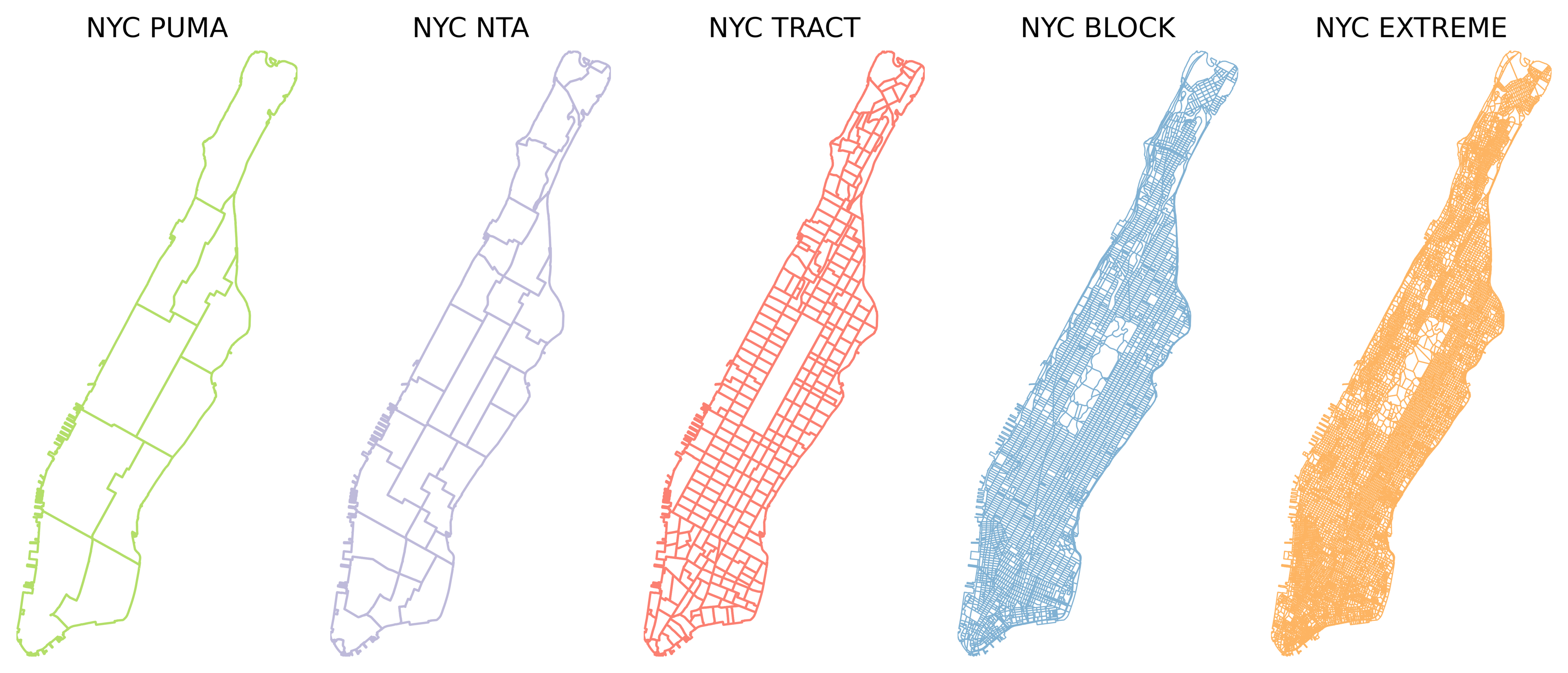
Figure 2. Five distinct geographic aggregation levels for the same NYC area. PUMA regions are largest and EXTREME regions are smallest.

3.1. Data Processing

We construct two representations of aggregated spatiotemporal event data: vector and raster. Given a dataset of individual events $(lat,lon,time)$, the two representations are constructed as follows.

Vector

We aggregate the event counts by hour and region for each of the five geographic levels. For example, there are 10 Public Use Microdata Areas (PUMA); a single hour of data is represented as simply a 10-element vector. The order of elements is arbitrary. More generally, the dataset is represented as $X\in\mathbb{R}^{N\times d}$, where $N$ is the total number of hours, and $d$ is the number of regions at a given geographic level (e.g., $d$ = 10 for PUMA; $d$=32 for NTA).

Raster

We first define a 128$\times$256 grid and plot the $N$ regions at each geographic level. Each region has a corresponding value from the vector input — $X_{n},n\in\{1,2,\dots,N\}$, and the number of pixels located within the region — $C_{n},n\in\{1,2,\dots,N\}$. Then each pixel in each region takes the value of $\frac{X_{n}}{C_{n}}$. For pixels that are shared by more than one regions, we assign them to the smaller regions to avoid overlapping issue. This representation captures the shape of, and spatial relationships between, individual regions and affords the use of convolutional layers to model local and non-local influences. The cost is that we lose information during translation since the raster representation does not represent region boundaries precisely, especially at BLOCK and EXTREME level.

3.2. Data Statistics

We computed descriptive statistics, including means and standard deviations, for the counts of each dataset at different geographic levels. These statistics are shown in Table 1. The standard deviations are large demonstrating the significant variability in the count values between regions. For instance, Inwood in upper Manhattan have considerably fewer taxi rides compared to the more central areas of Manhattan. In the case of the NYC 911 Call and Chicago Taxi data, we notice significantly smaller average values at the BLOCK and EXTREME levels. This observation can be attributed to the nature of emergency incidents and taxi demand, which may vary in frequency across different regions within the city. As a result, the average values of these datasets are lower at the more granular levels. For all three NYC datasets, we use the month of June as the test split, the month of May as the validation split, and the rest as training data. For Chicago taxi data, we use the month of December as the test split and November as the validation split, and the rest as training data.

Data	PUMA	NTA	TRACT	BLOCK	EXTREME
NYC Taxi	1443.01	450.94	50.99	3.85	1.27
	(1776.03)	(689.15)	(73.26)	(8.02)	(3.59)
NYC Bikeshare	189.53	59.23	6.7	0.5	0.17
	(279.24)	(97.86)	(13.06)	(2.53)	(1.41)
NYC 911 Call	23.25	7.27	0.82	0.06	0.02
	(14.22)	(7.05)	(1.34)	(0.32)	(0.19)
Data	COM	TRACT	BLOCK	EXTREME	-
Chicago Taxi	27.71	2.39	0.06	0.04	-
	(64.61)	(10.91)	(1.7)	(1.35)	-

Table 1. Descriptive statistics of four datasets. The numbers are the average hourly taxi/bike/call counts per geographic region. The standard deviations are in the parenthesis.

4. Models

In this section, we will begin by providing an overview of the traditional methods commonly employed for the task of disaggregation. Following that, we will articulate the details of our proposed COT architecture and REC loss. The traditional methods are consider as baseline models to be compared against.

4.1. Baseline Models

As our baseline, we tested several simple, traditional disaggregation methods, as well as neural models:

• Constant Weighting (CW): The event count for a region in the output is assumed to be $\frac{1}{N}$ of the count in the containing region in the input, where $N$ is the number of output regions contained in the input region. That is, this heuristic assumes the events are uniformly distributed, regardless of size and shape of the region.

• Areal Weighting (AW): The event count for an output region $r$ contained in an input region $c$ is assumed to be proportional to the fractional area of $r$ in $c$. That is, $|r|=\frac{A(r)|c|}{A(c)}$, where $A(r)$ is the area of region $r$ and $|c|$ is the event count in region $c$. That is, this heuristic assumes events are uniform per unit area.

• Historical Ratios (HR): The event count of an output region $r$ is assumed to be a fixed proportion of the count of an input region $c$. The fixed proportion is computed as the average proportion from all historical timesteps.

• Feedforward Neural Network (FNN): The event count for an output region $r$ is assumed to be a (non-linear) function of all input regions, not just the containing region. The function is modeled as a multi-layer feedforward neural network trained on historical data. This approach attempts to capture the interdependencies between regions: high traffic at Penn Station can correlate with high traffic in the upper east side, for example.

• Convolutional Neural Network (CNN): The event count at each output region $r$ is extracted from the raster representation at the output aggregation level (e.g., city blocks). That raster representation in turn is learned from the raster representation of the input aggregation level (e.g., PUMA) using a typical UNet architecture (Ronneberger et al., 2015). This approach models the non-linear relationships between regions, while emphasizing local effects through convolutional layers.

• Long Short Term Memory (LSTM): Where FNN only models the spatial connections (by assuming that each timestep is an independent smaple), LSTM can capture temporal patterns. We chose T=5 as the temporal sequence length across all our experiments based on the study (Han and Howe, 2023). Otherwise, this model is similar in inputs and outputs to FNN.

4.2. Chain of Training (COT)

Across all methods, the error is influenced by the difference between the input and output resolutions: Given PUMA data, it is harder to predict accurate values at the city block level than at the census tract level. Based on this observation, we considered that constraining the model to learn accurate intermediate aggregations, step-by-step, could improve performance. We therefore employ a spatially coherent architecture design that is compatible with any multilayer network using the vector representation (FNN, LSTM), where selected layers in the network correspond to real aggregation layers. We then introduce a new loss term for each spatially coherent layer to encourage the model to make accurate predictions at the intermediate steps as well as the final output. These loss terms are simple to implement, since we have access to ground truth at all levels simultaneously, as with other hierarchical models in computer vision (Ying et al., 2019; Wurster et al., 2022) or time-series modeling (Taieb et al., 2017; Abolghasemi et al., 2019). This architecture and corresponding loss terms encourage the model to ”show its work” in computing the final output.

We propose a training strategy called Chain-of-Training (COT), invoking the similar concept of chain of thought in LLM prompt engineering. This approach provides several benefits: 1) The final predicted output is penalized if it is inconsistent with intermediate results, 2) the overall performance is (as we will show) improved, 3) multiple aggregation levels can be predicted in a single model, if desired, reducing training time (at a small cost in accuracy), and 4) spatially coherent layers trained separately (using potentially different architectures) can be meaningfully spliced together into a single model post hoc, since they have a common real-world interpretation that is independent of the architecture or training regime. See Figure 3 for an illustrative example involving FNN.

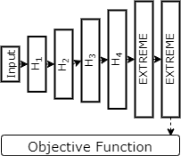
(a) FNN

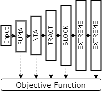
(b) FNN + COT

Figure 3. FNN model architectures to disaggregate from PUMA to EXTREME level. (a) the architecture of a regular FNN model. The hidden dimensions could be of any values. We only calculate the loss using the output from the last layer. (b) The four hidden layers have the dimension sizes that are equal to the number of regions at PUMA, NTA, TRACT, and BLOCK levels. We calculate losses at those four levels, as well as the last layer.

We adopt the following notation to discuss the objective function:

• $g_{i}$ for $i\in\{0,1,\dots,N\}$ denotes a geographic aggregation level. The levels are labeled in ascending order in terms of number of regions, i.e., the lowest resolution is assigned 0 and the highest resolution is assigned $N$. In our experiments, the input is always the lowest resolution, e.g. PUMA for NYC. Therefore, it is assigned with the categorical level $g_{0}$. Level $g_{N}$ has the largest number of regions, which is EXTREME. Level $(g_{1},g_{2},\dots,g_{N-1})$ are intermediate levels.

• $|g_{i}|$ denotes the number of regions at geographic level $g_{i}$

• $|g_{b}|$ denotes the number of regions at the BLOCK level, which we use to normalize the loss terms, as described next.

• $x_{i}\in\mathbb{R}^{|g_{i}|}$ denotes the ground truth vector at geographic level $g_{i}$. We sometimes include a superscript $(n)$ to denote the $n$th sample.

• $\hat{x}_{i}\in\mathbb{R}^{|g_{i}|}$ denotes a prediction of the disaggregated vector at geographic level $g_{i}$. The model used to make the prediction will be clear from context. Each model is capable of making predictions at any level. We sometimes include a superscript $(n)$ to denote the $n$th sample.

Ensuring compatible loss units

With COT, we calculate losses at the target aggregation level as well as all intermediate levels. These losses are combined and back-propagated jointly. L1 loss is frequently used for disaggregation accuracy. However, since L1 loss divides by the size of the vector, meaning that the L1 loss will have different units at each aggregation level and cannot be meaningfully combined. For example, the L1 loss $\frac{|\hat{x}_{i}-x_{i}|}{|g_{i}|}$ at the TRACT level is in units of ”events per TRACT region” while the L1 loss at the BLOCK level is in units of ”events per BLOCK region.” The loss at $g_{0}$ will be incomparable to the loss at, say, $g_{4}$. Therefore, we normalize all loss terms to be events-per-region at a selected aggregation level. In our experiments, we normalize to the BLOCK level to assist with interpretation: we consider taxi rides per city block as more familiar than taxi rides per PUMA region, for example.

For non-COT models (e.g., baseline FNN and LSTM), we use the following loss as the objective function at the target level $g_{i}$:

(1) $$COT_{i}=\frac{1}{|g_{b}|}\sum_{n=0}^{|g_{i}|-1}|\hat{x}_{i}^{(n)}-x_{i}^{(n)}|$$

With COT models, which combines losses at fine and intermediate levels, the objective function is:

(2) $$\mathcal{L}_{COT}=\alpha_{0}COT_{0}+\alpha_{1}COT_{1}+\dots+\alpha_{N}COT_{N}$$

where $\alpha_{i}$ is a hyperparameter weight for geographic level $i$. We will describe a how to set these weights deterministically, without tuning, in Section 4.4.

4.3. Reconstruction Loss (REC)

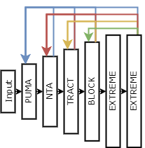
(a)

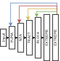
(b)

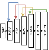
(c)

Figure 4. Three reconstruction schemes involving different subsets of the $\frac{n(n-1)}{2}$ possibilities. (a) Full reconstruction: each level $k$ is used to reconstruct all previous levels $i<k$. (b) BottomUp reconstruction: the output at level $N$ is used to reconstruct all previous levels $i<N$. (c) Bridge reconstruction: each level $i$ is only used to reconstruct its immediate predecessor at level $i-1$.

The disaggregation task shares similarities with the super-resolution task, which aims to recover high-resolution images from their corresponding low-resolution counterparts. While supervised methods are commonly used in this domain, there are also weakly- or unsupervised approaches (Wang et al., 2020). Yuan et al.(Yuan et al., 2018) introduced a cycle-in-cycle framework to facilitate the learning of mappings between low-resolution and high-resolution images, as well as the reverse mappings from high-resolution to low-resolution. This framework enables the model to capture the underlying relationships between the two resolution levels by leveraging the concept of cycle consistency. Cycle consistency refers to the idea that if we transform a low-resolution image to the high-resolution domain and subsequently transform it back to the low-resolution domain, the resulting image should ideally be similar to the original high-resolution image. This principle holds true in the reverse direction as well. By incorporating cycle consistency into the training process, the model is encouraged to generate outputs that are coherent and consistent across different resolutions.

In our disaggregation task, we adopt a similar reconstruction (REC) process: we predict the output aggregation level (say, BLOCK) with a forward pass, then re-aggregate to produce predictions at intermediate levels (TRACT, NTA, PUMA). These reconstructed predictions can then be compared with ground truth or with the predictions from the forward pass to produce additional loss terms. In our experiments, we only compare with ground truth. These reconstruction loss terms, in contrast to the core loss terms from COT, help ensure self-consistency, because an invariant of the disaggregation problem is conservation of events: the total events in region $c$ at level $i$ should equal the sum of events in regions $r_{0},r_{1},...,r_{n}$ at level $i+1$ contained in $c$. Given the containment property, these reconstruction terms are straightforward to compute. If the containment property does not hold, meaning that a region $r$ at level $i+1$ may not be wholly contained in any region at level $i$, the computation involves finding the intersection of polygons and allocating events proportionally by area. In our domains, the containment property holds. Then any aggregation level $g_{k}$ can be used to reconstruct any level $g_{i}$ for $i<k$, generating $\frac{n(n-1)}{2}$ possible new loss terms. We consider three reconstruction strategies using subsets of these loss terms in our evaluation:

• REC-Full: Each aggregation level $k$ is used to reconstruct all aggregation levels $i<k$. The average loss of all reconstructions for each level $i$ is then included in the loss function. For example, in Figure 4(a), the reconstructed PUMA values are from NTA, TRACT, BLOCK, and EXTREME (shown as blue lines). The intuition is to penalize any divergence from self-consistency among intermediate levels, at the risk of involving too many competing objectives that need to be balanced.

• REC-BottomUp: The final output at level $n$ is used to reconstruct all previous levels $i<n$, but no other reconstructions are used. The intuition is that we want to constrain the final output as much as possible and relax conditions on the intermediate levels. See Figure 4(b).

• REC-Bridge: Each level $i$ is only used to reconstruct its immediate predecessor at level $i-1$. For example, we use BLOCK to reconstruct TRACT, but not NTA. The intuition is reduce the total number of competing objectives but still ensure consistency between intermediate levels. See Figure 4(c)).

Example: Full Reconstruction Loss

We adopt the following additional notation to discuss the objective functions:

• $M_{i,j}$ is an $|g_{i}|\times|g_{j}|$ binary matrix representing the containment relationship between aggregation levels $g_{i}$ and $g_{j}$. A value of 1 at position $M[c,r]$ indicates that region $r$ at level $j$ is contained in region $c$ at level $i$.

• $\hat{x}_{j\rightarrow i}$ for $i<j$ is the reconstructed vector at geographic level $g_{i}$ using the prediction at level $g_{j}$, that is $\hat{x}_{j\rightarrow i}=M_{i,j}\hat{x}_{j}$

The REC loss at level $g_{i}$ from level $g_{j}$ is the sum of errors divided by the number of reference regions (city blocks in our experiments):

(3) $$REC_{j\rightarrow i}=\frac{1}{|g_{b}|}\sum_{n=1}^{|g_{i}|}|\hat{x}_{j\rightarrow i}^{(n)}-x_{i}^{(n)}|$$

The combined REC loss at level $g_{i}$ from all higher levels is:

(4) $$REC_{i}=\sum_{j=i+1}^{N}REC_{j\rightarrow i}$$

In the final objective function in the full reconstruction case, we sum estimates for each level $i$. The estimate at level $i$ is the average of all predictions for level $i$, including the core COT prediction. Specifically:

(5) $$\mathcal{L}_{\textit{COT+Full}}=\sum_{i=0}^{N-1}\frac{\alpha_{i}}{N-i+1}\left(COT_{i}+\sum_{j=i+1}^{N}REC_{j\rightarrow i}\right)$$

For the other reconstruction schemes, the loss functions are similar, only varying in the which REC terms we include:

(6) $$\mathcal{L}_{\textit{COT+Bottomup}} =\sum_{i=0}^{N-1}\frac{\alpha_{i}}{N-i+1}\left(COT_{i}+REC_{N\rightarrow i}\right)$$

(7) $$\mathcal{L}_{\textit{COT+Bridge}} =\sum_{i=0}^{N-1}\frac{\alpha_{i}}{N-i+1}\left(COT_{i}+REC_{i+1\rightarrow i}\right)$$

4.4. Weighting Loss Terms

In our final objective function, we combine losses from different levels together. However, as mentioned in §4.2, the error scales with the target resolution (as one would expect). Consequently, the loss from the EXTREME level can overwhelm the losses from other levels. In preliminary experiments, the error at the EXTREME level was 10X that of the PUMA level. When we used L1 error (without normalizing to BLOCK), the opposite occurred: error at the lower resolution levels would dominate those at the higher resolution by a factor of up to 100x. To counteract this imbalance, we normalize to BLOCK as described in Section 4.2, but we also derive weights for the loss terms based on ratios between the numbers of regions. These ratios scale approximately exponentially in the level $i$: Each region at level $i$ tends to be split into about 2-3 regions at level $i+1$. We therefore compute weights as the logarithm of the ratios to counteract this growth. Specifically:

$$\alpha_{i}=log_{2}(\frac{|g_{N}|}{|g_{i}|}),i\in\{0,1,\dots,N-1\},\;\;\;\alpha_{N}=1$$

By assigning higher weights to the losses from coarser levels with fewer regions, we effectively emphasize their importance in the learning process. This approach helps to balance the contributions from different levels and encourage accurate predictions at intermediate levels, which in turn produces more accurate output predictions. We report on an ablation study in Section 5.2.

For NYC data, all disaggregation tasks start from PUMA level to NTA, TRACT, BLOCK, and EXTREME levels. Therefore, we have four disaggregation tasks. Likewise, we have three disaggregation tasks for Chicago taxi data, which all start from COM level. All training-based models are trained with the training set and monitored with the validation set. The batch size is 8 and learning rate is 1e-4. We use early stop setting to prevent over-fitting the training data. The final results are reported on the held-out test set. The errors are calculated with Equation 1, with the unit of “per block, per hour”. The unit provides easier interpretation and allows the comparison of results across different disaggregation resolutions.

4.5. Training Regimes

We propose three training regimes for the disaggregation models: 1) Separate Training: train separate models for each target level. 2) Joint Training: train one overall model that disaggregates from PUMA to EXTREME. This model can be used to produce estimates at all levels simultaneously. 3) Layer-by-Layer Training: a layer-by-layer training process where each aggregation level is trained then frozen before adding the next level and repeating the process. For example, we first train the model to disaggregate from PUMA to NTA, the layers of which are used to initiate the model that disaggregates from PUMA to TRACT and kept frozen (not updated through back-propagation). We repeat the same process for BLOCK and EXTREME level disaggregation. Our spatially coherent architecture COT enables this layer-by-layer training strategy .

4.6. Transfer Learning

As mentioned in §1, we do not always have access to complete historical data for training. In these cases, we can consider whether a model pre-trained on one variable can be used to make predictions for another variable. We can use our models in this transfer learning setting by training on, say, taxi data, then fine-tuning on a limited amount of bikeshare or 911 data. This approach can significantly increase the value of open data, by allowing one dataset to be used in different applications. The idea is reasonable, given the interconnectedness of city dynamics as a complex system (Howe et al., 2022): everything depends on everything else. Moreover, the main signals being learned by any model are influenced by the built environment, human activity, and population density patterns, all of which tend to be exhibited in any spatiotemporal dataset in the same domain.

4.7. Event Data Synthesis

While the EXTREME aggregation level are high-resolution (smaller than city blocks) they are still spatially aggregated and cannot be directly used by applications expecting individual event data. A simple approach is to use COT to learn a high-resolution aggregation, then simply sample these regions to generate individual points. If a region has $k$ events, we can sample $k$ events at random locations within its boundaries. Although this simple approach will violate the constraints of the built environment (e.g., locating taxi-rides within hotel lobbies) it is simple to compute and can be controlled by the aggregation levels.

Quality control is important for the synthesized data. Quantitatively, we can compare the distributions of real and synthesized points over the extreme regions. Two statistics are appropriate to measure their similarities — Mutual Information (MI) and KL-divergence statistics. MI measures the probabilistic dependency between two variables. The higher the value, the more information the two variables share between each other. In other words, knowing one of the two variables reduces the uncertainty about the other. KS statistics is used to test the null hypothesis that two independent samples are drawn from the same continuous distribution. In our case, we want to test whether the two taxi frequency distributions are from the same distribution. KL divergence is a a measure of entropy increase due to the use of an approximation distribution to the true distribution rather than the true distribution itself. Qualitatively, we can visualize the distributions of real and synthesized points. Some notable patterns (e.g., clustering) and discrepancies can be compared.

5. Experimental Results

In this section, we present our experimental results that answer the following questions:

1. Do neural methods improve performance over conventional heuristic methods? (Yes) (Section §5.1)

2. Does the proposed COT strategy improve performance? (Yes) Do REC losses improve performance? (Sometimes) Which REC  scheme works the best? (BottomUp) Is the weighting scheme effective? (Yes, and is required) (Section §5.2)

3. How do different training regimes (separate models, joint model, layer-by-layer) balance tradeoffs between error and training time? (Separate models are lowest error, but slowest; layer-by-layer outperforms joint model and significantly reduces training time) (Section §5.3)

4. Can we fine-tune a disaggregation model trained on one variable and have it perform competitively on a differnet variable? (Yes) (Section §5.4)

5. Can disaggregation models synthesize realistic individual events from aggregated values? (Yes) (Section §5.5)

5.1. Neural Outperforms Classical Methods

Figure 5 visualizes the errors of the disaggregation task using both classical and neural methods. We observe that — 1) As the target disaggregation resolution increases, the error increases across all methods, as expected. Predicting city block dynamics from large regional aggregates is a difficult problem. 2) Heuristic-based disaggregation methods, such as CW (Constant Weighting) and AW (Areal Weighting), are non-competitive across all resolutions and datasets. The underlying heuristics are reasonable but cannot capture the dynamics at higher resolution. The distribution of taxi rides, bikeshare trips, and 911 calls follows human activity patterns, which are influenced by the built environment, temporal effects, and non-linear interactions between regions. 3) The HR (Historical Ratio) method demonstrates significant performance improvement over the heuristic methods. This improvement can be attributed to the ability of HR to capture temporal patterns from historical data. However, HR still overlooks the non-linear temporal and spatial variations present in the data, limiting its overall accuracy. 4) Neural-based methods outperform the simple methods in almost all disaggregation tasks. LSTM models, in particular, show superior performance compared to models that solely rely on spatial information, since the LSTM models capture the non-independence of the timesteps. LSTM emerges as the best-performing baseline model among all tested methods. CNN models exhibit worse performance than HR models when disaggregating from PUMA to EXTREME resolution, particularly in the case of NYC taxi and bikeshare datasets. This performance discrepancy can be attributed to the loss of information that occurs during the conversion from vector inputs to image representations in CNN models. Overall, the results show that learning from historical data, especially LSTM models, improves performance for this task.

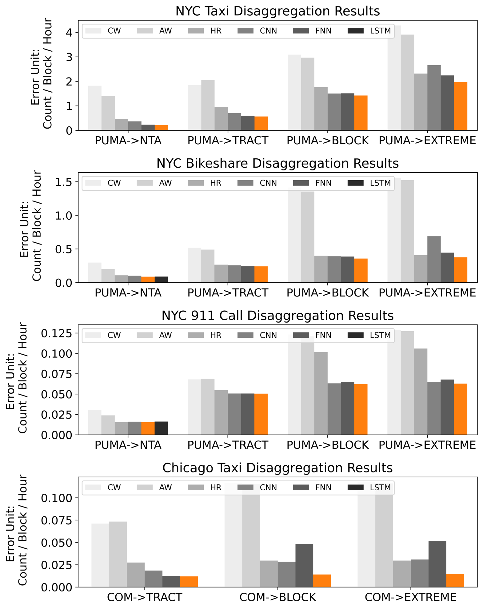
Figure 5. Disaggregation results from heuristic and neural models on four datasets. X-axis is the target disaggregation level. Y-axis is the error in number events per city block per hour. Different colors indicate different models; orange indicates best.

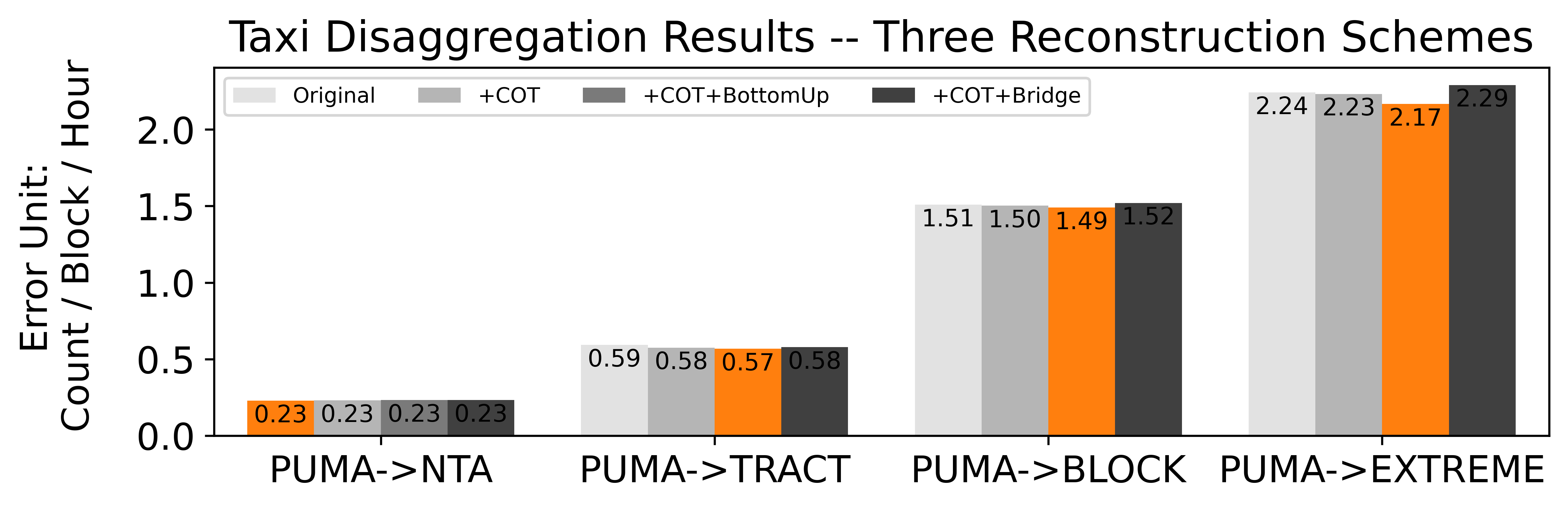
Figure 6. Disaggregation results for different reconstruction schemes on NYC Taxi dataset. X-axis shows the disaggregation resolutions. Y-axis shows the error per city block, per hour. Different color represents different reconstruction methods; orange is best.

5.2. COT & REC Improve Neural Results

Full and BottomUp reconstruction improve performance situationally

We trained FNN models using COT and the three reconstruction methods. The results are visualized in Figure 6. +COT+Bridge yields worse results compared to the plain results across all tasks. We conjecture that since the last layers in any model are those that are most influenced by training, the reconstructions at the early layers used by bridge are not engaging with the training process as much, confounding the model. +COT+Full achieves the best performances when disaggregating from the PUMA to BLOCK resolution. +COT+BottomUp outperforms the other two schemes when disaggregating from the PUMA to TRACT and EXTREME. Both +COT+Full and +COT+BottomUp improve performance and are comparable. We conjecture that reaggregating from the EXTREME level, where error is highest, is most responsive to backlpropagation. In the following, we present results from only these two schemes.

The weighting scheme mediates performance

In §4.4 we derived a weighting scheme to balance the losses of different geographic levels. We trained FNN with COT and REC  with and without the weighting; results appear in Table 3. The PUMA $\rightarrow$ NTA task (the lowest resolution) does not benefit, since there is only one loss term such that relative weighting has no effect. For the three other tasks (PUMA to TRACT, BLOCK, and EXTREME), the weighted models outperform their unweighted counterparts. The unweighted models are worse than the baseline in some cases, suggesting overfitting. Overall, the deterministic weighting scheme mediates performance when including the additional loss terms, since the error scales exponentially with the geographic aggregation level (each region at level $i$ splits into approximately 2-3 regions at level $i+1$).

Main result: COT & REC improve neural results

For our main result, we trained FNN and LSTM models with COT, COT+Full and COT+BottomUp across all datasets, using the area-aware weighting scheme. For statistical significance tests, we use bootstrap sampling for 10,000 iterations (Jurafsky and Martin, 2008; Sonderegger and Buscaglia, 2020): On each iteration, we sample the predictions, then calculate error and compute the proportion that are better than the baseline to provide an empirical estimate of the p-value. We use 0.05 as the significance level. Table 2 shows the results. With the NYC taxi dataset, COT results consistently outperform the baseline results in most disaggregation tasks, except for the PUMA to NTA task. Both COT+Full and COT+BottomUp further improve the results significantly. The LSTM model equipped with our improvements are consistently best.

COT alone also outperforms the baseline results, except for the PUMA to NTA task. For the other three datasets (NYC bikeshare, NYC 911 call, and Chicago taxi), the COT results usually outperform the plain results in all disaggregation tasks, and the differences are statistically significant. In the two tasks where the baseline results are better (NYC 911 call, LSTM, PUMA to BLOCK/EXTREME), the differences are insignificant. The inclusion of either Full or BottomUp reconstruction strengthens the performance in some tasks, but not consistently. REC loss terms in some cases decreases performance, particularly with the NYC bikeshare and 911 call datasets. The NYC taxi and bikeshare datasets involve higher resolution targets, a more difficult task. The magnitude of the difference between the baseline result and our results tends to increase, with two exceptions at the EXTREME level, suggesting that the harder the task, the more these methods help.

Overall, COT consistently improves disaggregation results across different datasets and tasks. The incorporation of Full or BottomUp reconstruction schemes generally improves performance further, but not always. The magnitude of the improvement and the varying effects of the REC schemes depend on the specific dataset, disaggregation task, and model configuration.

Different Cities and Domains Have Impacts on the Results

Our selection of four real datasets allowed us to explore multiple experimental conditions, including same city and same application domain (NYC taxi and NYC bikeshare), same city and different application domain (NYC taxi/bikeshare and NYC 911 call), and different cities with either the same or different application domains (NYC taxi/bikeshare/911 call and Chicago taxi). Based on the results presented above, we observe that: 1) Same city, same domain (taxi, bikeshare): The results consistently showed similar patterns across both datasets. The COT strategy consistently produced the best results, demonstrating its robustness and effectiveness. Additionally, incorporating the REC losses situationally improved the performance of COT even further. Furthermore, fine-tuning the taxi models on the bikeshare data yielded competitive results, indicating the potential for cross-domain learning within the same city. 2) Same city, different domain (taxi, 911 call): In this scenario, COT still emerged as the top-performing method on both datasets. However, the REC  losses did not consistently enhance the results on the 911 call data and occasionally led to worse performance. This suggests that our proposed approaches may be more compatible with mobility-related data rather than emergency call data. Nevertheless, fine-tuning the taxi models on the 911 call data showed promising results, indicating that even with different domains, datasets from the same city share common underlying urban dynamics, such as population activity. 3) Different city, same or different domain (NYC taxi/bikeshare/911 call, Chicago taxi): In this case, COT consistently outperformed other methods on all datasets, affirming the robustness and city invariance of COT ’s performance. This finding indicates that our proposed methods are compatible with different city structures and can effectively handle disaggregation tasks in various urban environments.

Dataset	Model	Resolutions	Plain	+COT	+COT +BottomUp	+COT +Full	Diff
NYC Taxi	FNN	PUMA $\rightarrow$ NTA	0.2276	0.2302	0.2328	0.2328	-0.0026
		PUMA $\rightarrow$ TRACT	0.5927	0.5752*	0.5679*	0.5695*	+0.0248
		PUMA $\rightarrow$ BLOCK	1.5090	1.5023*	1.4908*	1.4890*	+0.0200
		PUMA $\rightarrow$ EXTREME	2.2425	2.2328*	2.1683*	2.2025*	+0.0742
	LSTM	PUMA $\rightarrow$ NTA	0.2097	0.2101	0.2084	0.2084	+0.0013
		PUMA $\rightarrow$ TRACT	0.5621	0.5448*	0.5392*	0.5429*	+0.0230
		PUMA $\rightarrow$ BLOCK	1.4215	1.4136*	1.3813*	1.3926*	+0.0401
		PUMA $\rightarrow$ EXTREME	1.9699	1.9546	1.9588	1.9540*	+0.0159
NYC Bikeshare	FNN	PUMA $\rightarrow$ NTA	0.0868	0.0806*	0.0815*	0.0815*	+0.0063
		PUMA $\rightarrow$ TRACT	0.2417	0.2314*	0.2302*	0.2321*	+0.0114
		PUMA $\rightarrow$ BLOCK	0.3861	0.3675*	0.3886	0.3913	+0.0186
		PUMA $\rightarrow$ EXTREME	0.4452	0.4224*	0.4501	0.4456	+0.0227
	LSTM	PUMA $\rightarrow$ NTA	0.0891	0.0830*	0.0825*	0.0825*	+0.0066
		PUMA $\rightarrow$ TRACT	0.2412	0.2335*	0.2337*	0.2316*	+0.0095
		PUMA $\rightarrow$ BLOCK	0.3572	0.3447*	0.3610	0.3585	+0.0125
		PUMA $\rightarrow$ EXTREME	0.3749	0.3688*	0.4497	0.3805	+0.0060
NYC 911 Call	FNN	PUMA $\rightarrow$ NTA	0.0156	0.0156	0.0157	0.0157	0.0000
		PUMA $\rightarrow$ TRACT	0.0506	0.0502*	0.0531	0.0531	+0.0004
		PUMA $\rightarrow$ BLOCK	0.0649	0.0638*	0.0913	0.0884	+0.0011
		PUMA $\rightarrow$ EXTREME	0.0678	0.0667*	0.0956	0.0952	+0.0011
	LSTM	PUMA $\rightarrow$ NTA	0.0162	0.0156*	0.0156*	0.0156*	+0.0006
		PUMA $\rightarrow$ TRACT	0.0505	0.0502*	0.0530	0.0527	+0.0003
		PUMA $\rightarrow$ BLOCK	0.0624	0.0625	0.0913	0.0894	-0.0001
		PUMA $\rightarrow$ EXTREME	0.0628	0.0630	0.0958	0.0950	-0.0001
Chicago Taxi	FNN	COM $\rightarrow$ TRACT	0.0126	0.0125	0.0127	0.0127	+0.0001
		COM $\rightarrow$ BLOCK	0.0484	0.0193*	0.0214*	0.0211*	+0.0290
		COM $\rightarrow$ EXTREME	0.0519	0.0223*	0.0242*	0.0413*	+0.0296
	LSTM	COM $\rightarrow$ TRACT	0.0120	0.0114*	0.0117*	0.0115*	+0.0005
		COM $\rightarrow$ BLOCK	0.0140	0.0130*	0.0145	0.0140	+0.0010
		COM $\rightarrow$ EXTREME	0.0147	0.0133*	0.0143*	0.0138*	+0.0013

Table 2. Disaggregation results of plain neural models and our proposed COT strategy and REC losses. The unit of the error is count/block/hour. Bold numbers indicate the best result in the corresponding disaggregation task. * indicates statistical significance test from bootstrap sampling. {Diff} column presents the difference between Plain results and the best result of {+COT, +COT+Full, +COT+BottomUp}. Positive difference means improvement.

Dataset	Resolutions	FNN	+COT	+COTW	+COT +BottomUp	+COT +BottomUpW	+COT +Full	+COT +FullW
NYC Taxi	PUMA $\rightarrow$ NTA	0.2276	0.2313	0.2302	0.2308	0.2328	0.2308	0.2328
	PUMA $\rightarrow$ TRACT	0.5927	0.5773	0.5752	0.5739	0.5679	0.5715	0.5695
	PUMA $\rightarrow$ BLOCK	1.5090	1.5157	1.5023	1.5449	1.4908	1.5884	1.4890
	PUMA $\rightarrow$ EXTREME	2.2425	2.2045	2.2328	2.2849	2.1683	2.3131	2.2025

Table 3. Disaggregation results of weighted and unweighted models. The column with the $\{\}^{W}$ indicates the results from weighted models, while the other column shows the unweighted results. Underlined numbers are the better ones within each pair of unweighted and unweighted results. The unit of the error is count/block/hour.

Dataset	Resolutions	FNN+COT			FNN+COT+Full			FNN+COT+BottomUp
NYC Taxi		Separate	Joint	Layer- by-Layer	Separate	Joint	Layer- by-Layer	Separate	Joint	Layer- by-Layer
	PUMA $\rightarrow$ NTA	0.2607(16)	0.4497(-)	0.2607(15)	0.2662(14)	0.3502(-)	0.2662(13)	0.2662(14)	0.3770(-)	0.2662(13)
	PUMA $\rightarrow$ TRACT	0.6263(13)	0.8858(-)	0.6667(2)	0.6314(16)	0.7111(-)	0.6709(6)	0.6356(12)	0.8373(-)	0.6683(4)
	PUMA $\rightarrow$ NTA	1.7155(3)	1.9163(-)	1.7068(4)	1.6024(14)	1.8486(-)	1.6216(3)	1.5477(10)	7.6979(-)	1.5895(3)
	PUMA $\rightarrow$ NTA	2.8417(7)	2.8417(7)	2.8740(6)	2.5815(43)	2.5815(43)	2.5722(12)	2.3414(21)	2.3414(21)	2.4216(10)

Table 4. Evaluation of training regimes. The {Separate} column shows the results the models that are separately trained for each disaggreagtion task. The {Separate-Extraction} column shows the results by extracting and evaluating the intermediate outputs of the separatedly trained PUMA to EXTREME models. The {Layer} column shows the results of layer-by-layer training regime. The unit of the error is count/block/hour. The training time is included in the parenthesis.

5.3. Layer-by-Layer Training Significantly Reduces Training Time

We proposed three training regimes for our disaggregation models in Section §4.5: train separate models for each aggregation level, train one joint model to learn all levels simultaneously, and a layer-by-layer training regime. The results are reported in Table 4. Separately trained models for each task offer the lowest error, but are the most expensive to train. Training one joint model from PUMA to EXTREME and extracting intermediate results as predictions for the intermediate tasks is effective at reducing training time, but the error increases significantly. The layer-by-layer regime, freezing each intermediate layer after training, allows $N$ passes on the training data while significantly reducing training time in all cases. The results are competitive with the separately trained models, in two cases improving performance, suggesting that this training regime may be preferred in practical settings.

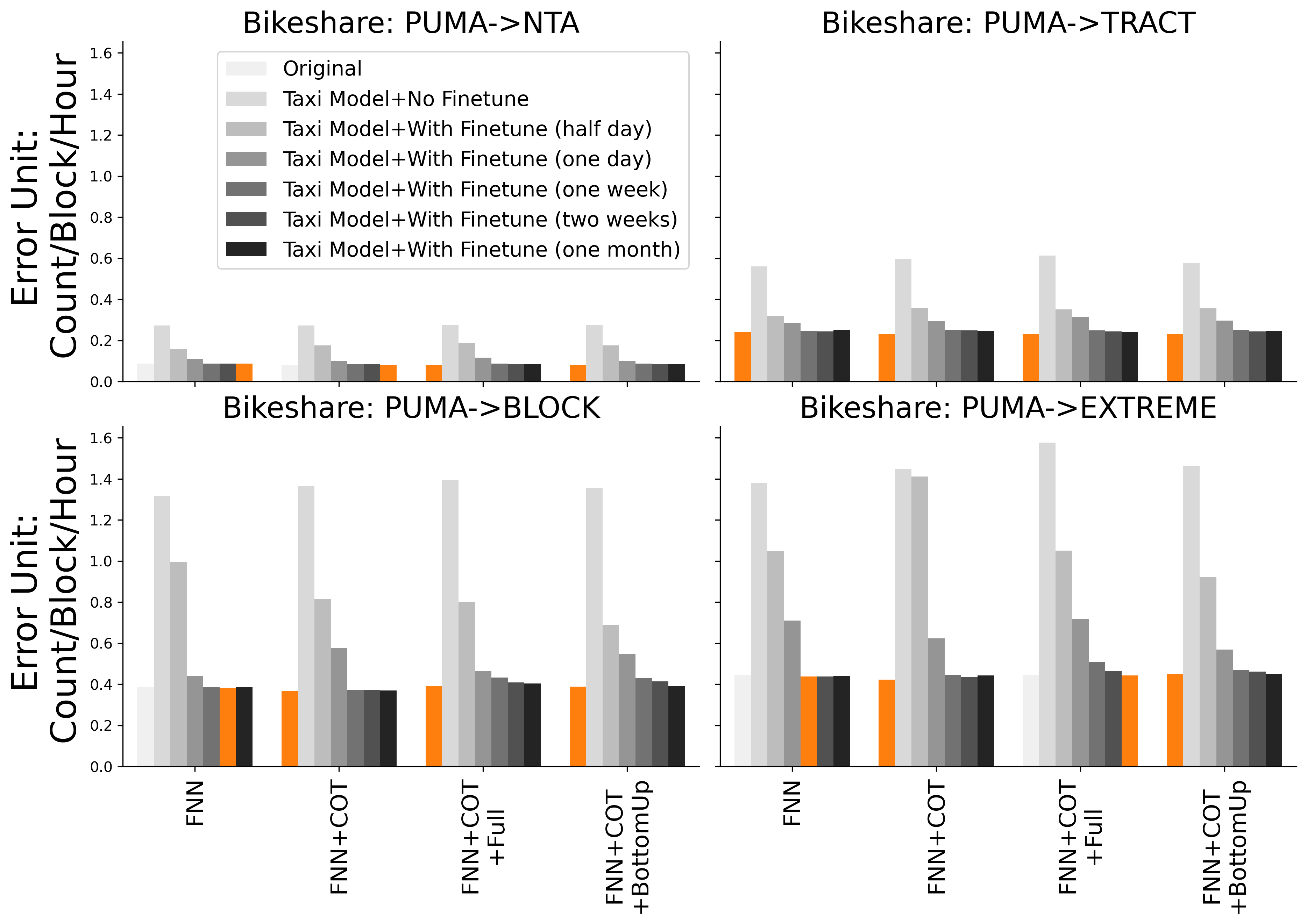
Figure 7. Transfer learning results when training on the NYC taxi dataset and fine-tuning (and evaluating) on bikeshare and 911-call datasets. Each subplot is a different disaggregation task. The X-axis is the model used, and each bar is a different amount of data used for fine-tuning. The unit of the error is count/block/hour. Orange indicates the best result.

5.4. Transfer Learning is Effective with Limited Fine-tuning

We trained FNN models on NYC taxi data and evaluated on bikeshare and 911-Call in the same NYC domain. We fine-tuned with a half day (12 hour-long samples), one day (24), one week (168 samples), two weeks (336), and one month (720). Figure 7 shows the results: Fine-tuning with only a week of data achieves results comparable with the specialized model trained from scratch on a full year. This result has significant implications for practical settings: Training data is not uniformly available for all variables due to technical, privacy, and political effects. But because cities are complex systems, all variables are interdependent (Howe et al., 2022). This result shows that pre-training can capture city dynamics resulting from the built environment and human activity, and that those signals tend to be predictive for multiple variables. We envision developing a core model with a large historical record, then fine-tuning for different tasks in the same city, analogous to a language model being fine-tuned for more specialized language tasks. Transfer learning across city domains, however, is an open problem.

5.5. Realistic Synthesis of Individual Events

In our experiments, we have assumed the desired output is still aggregated, just at a higher resolution. But many applications assume access to individual events (Zhang et al., 2020; Singh and Chen, 2023; Law et al., 2018). A simple strategy is to use uniform sampling of a high-resolution output to synthesize individual events. To test this approach, we use FNN to disaggregate PUMA to EXTREME with the NYC taxi data. Then, for each EXTREME region with $k$ events, we draw $k$ samples, each at a random location. Figure 8 shows an example of a set of regions in Manhattan. We draw samples from this set of regions to synthesize an individual dataset for two time periods on 06/01/2016, from 12AM-1AM and 12PM-1PM. We then measure the mutual information and KL divergence (using Python implementations) of the result distribution relative to the original distribution in the same time period and area. The results are reported in Table 5.

The normalized MI scores are 0.5430 and 0.7631 for the two time periods respectively. Both MI scores are higher than 0.5, indicating that two distributions share more than half their information. The KL-divergence are 0.4405 and 0.3941. Even with this naive sampling strategy, the KL divergence indicates a reasonable approximation: we would need about the same amount of auxiliary information to encode our predictions as the true distribution (0.39) as we would to encode the data from three hours later as the true distribution (0.31). Qualitatively, Figure 8 depicts the distributions of both real and synthesized taxi location points within the tract region at 12AM. The model generated slightly smaller numbers of taxi rides compared to the real counts, with differences of 12 rides. While these differences are present, they are not significant compared with all taxi counts within an entire tract region. In terms of the spatial distributions, the synthesized points capture the major clusters observed in the real taxi rides for both time periods, such as the clusters in the middle left and middle bottom areas. This suggests that the synthesized points closely approximate the general patterns and trends present in the real data. However, the synthesized points also scatter in regions where no real taxi rides can occur, making this simple approach unsuitable for some applications. A more sophisticated strategy would be to sample the areas with respect to the built environment.

Time	Normalized MI	KL-Divergence
12AM-1AM	0.5430	0.4405
12PM-1PM	0.7631	0.3941

Table 5. Statistics to measure similarities between two frequency distributions.

On the other hand, the presence of discrepancies between the real and synthesized data points can have benefits, particularly in terms of privacy protection. As highlighted in the introduction, individual privacy is a significant motivator for not releasing individual-level data. A closely matching distribution could be used as the basis of a privacy attack. For instance, clusters within very small areas may reveal the address of frequent riders. We consider our methods as providing better control over the tradeoffs between faithful distribution and privacy (though without formal privacy guarantees, which are atypical for transportation data anyway).

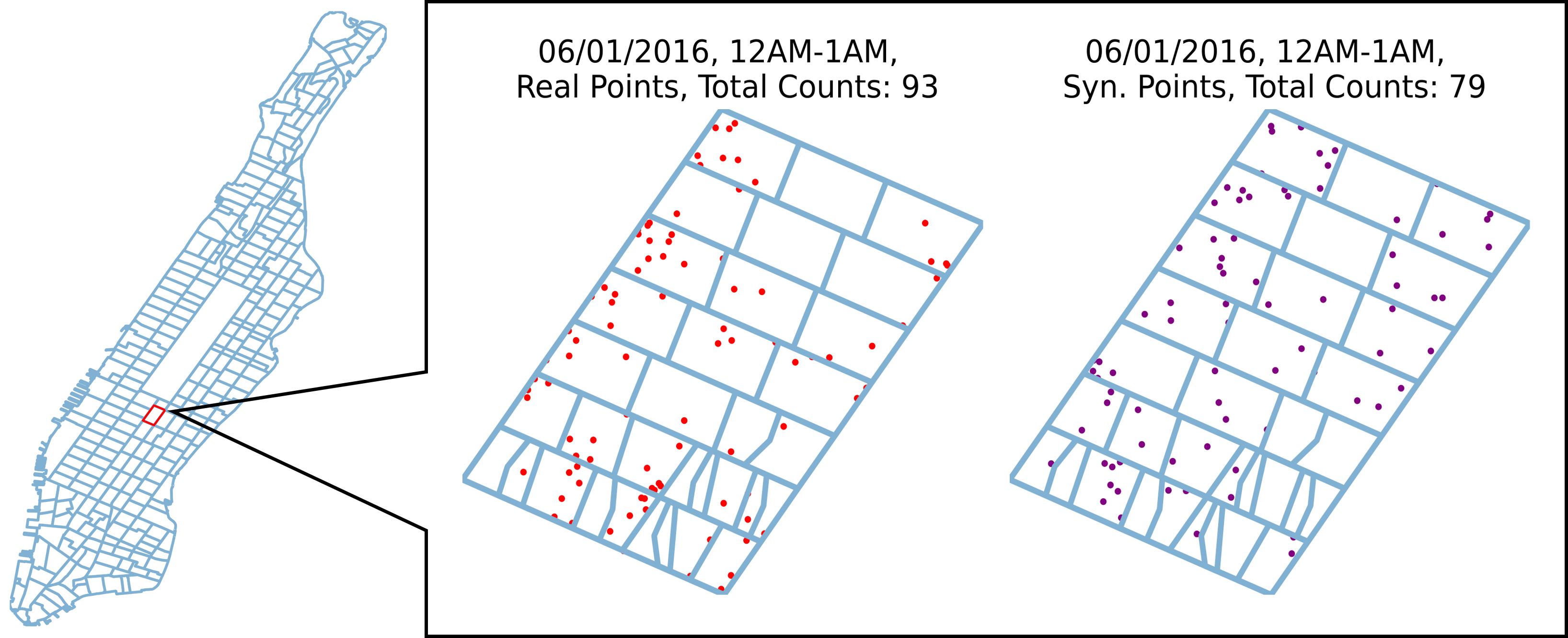
Figure 8. (Left) Randomly selected single tract region. (Right) The distributions of real and synthesized taxi rides are qualitatively similar.

6. Discussion and Conclusions

In this work, our objective is to synthesize high-resolution urban data by disaggregating low-resolution aggregated data. We considered various neural-based models capable of capturing non-linear relationships in space and time to improve over conventional heuristic methods in the literature. We demonstrated that all neural methods outperformed heuristic methods in almost all tasks, because real data violated the underlying assumptions: traffic and 911 calls are not uniformly distributed over subregions, nor do they scale based on area. By employing FNN and CNN models, we were able to capture spatial connections among different regions, while LSTM models further incorporated temporal interdependence such that LSTM models consistently produced the best results.

We introduced a spatially coherent architecture, where layers in the model correspond to real-world aggregation levels, along with a corresponding training strategy Chain-of-Training (COT), which penalized the model from allowing these intermediate layers from diverging from the ground truth too much. This approach explouts the fundamental properties of the problem: Given individual events, we can compute ground truth for any aggregation level needed. We also proposed Reconstruction (REC) losses, which reaggregate the output predictions to produce predictions at intermediate levels, which can then be compared with ground truth. This hierarchical approach allows us to optimize not only the loss at the final target level but also back-propagate the losses at the intermediate levels. Both COTand RECare compatible with any domain and any core architecture (e.g., LSTMs and CNNs). We also proposed a training regime to preserve performance while signfiicantly reducing training time, by training layer-by-layer, making a full pass on the training data for each layer, then freezing the weights and training the next layer. In this way, we make $N$ passes on the training data at a fraction of the training time.

Our experimental results consistently demonstrated the effectiveness of COT, with statistically significant enhancements observed in almost all tasks. The results for RECwere more situational, but typically outperformed baseline models with statistical significance. The layer-by-layer training offers competitive performance while significantly reducing training time.

Since not all variables are available with significant training data, we considered the transferability of a model trained on one variable for predictions on another (in the same city). With only a week of fine-tuning 911-Call data (168 samples), the taxi model exhibited performance comparable to that of the specialized model trained on longitudinal 911 call data. This result exposes that the underlying dynamics of human activity appear in all variables for the same city, opening new applications that integrate multiple data sources to overcome limited data availability (Khatiwada et al., 2022).

To produce the event-level data needed by some applications, we evaluated a naive method to synthesize individual points via uniform sampling within high-resolution regions. We show that the synthesized points have a similar distribution to the original, though they may violate constraints in the built environment. An improved synthesis model is left as future work.

There are some limitations to the study that we plan to address in future research: 1) The reliance on the containment property for the accurate reconstruction of fine values back to coarse values in our REC method. Currently, we assume that each region at level $i$ is contained in a region at level $i-1$, which disallows arbitrary partitionings of the domain. The basic concept of spatially coherent architectures and COTloss does not depend on this property, but our implementation and some aspects of RECdo. 2) Our current transfer learning experiments only consider scenarios where datasets are from the same city, meaning that they share the same geographic structures/grids. However, a practical situation may arise where one city has access to historical data that another city does not. Learning to ignore the influence of the built environment while retaining the dynamics of human activity is a challenging problem, but would dramatically increase the utility of open data by allowing cross-city models to be trained and learned.

References

- (1)
- Abolghasemi et al. (2019) Mahdi Abolghasemi, Rob J Hyndman, Garth Tarr, and Christoph Bergmeir. 2019. Machine learning applications in time series hierarchical forecasting. arXiv:1912.00370 [cs.LG]
- Arambepola et al. (2020) Rohan Arambepola, Tim C. D. Lucas, Anita K. Nandi, Peter W. Gething, and Ewan Cameron. 2020. A simulation study of disaggregation regression for spatial disease mapping. Statistics in Medicine 41 (2020), 1 – 16.
- Brauneck et al. (2023) Alissa Brauneck, Louisa Schmalhorst, Mohammad Mahdi Kazemi Majdabadi, Mohammad Bakhtiari, Uwe Völker, Jan Baumbach, Linda Baumbach, and Gabriele Buchholtz. 2023. Federated Machine Learning, Privacy-Enhancing Technologies, and Data Protection Laws in Medical Research: Scoping Review. J Med Internet Res 25 (30 Mar 2023), e41588. https://doi.org/10.2196/41588
- Burrell et al. (2004) J. Burrell, Tim Brooke, and R. Beckwith. 2004. Vineyard Computing: Sensor Networks in Agricultural Production. Pervasive Computing, IEEE 3 (02 2004), 38– 45. https://doi.org/10.1109/MPRV.2004.1269130
- Comber and Zeng (2019) Alexis J. Comber and Wen Zeng. 2019. Spatial interpolation using areal features: A review of methods and opportunities using new forms of data with coded illustrations. Geography Compass (2019), .
- Deville et al. (2014) Pierre Deville, Catherine Linard, Samuel Martin, Marius Gilbert, Forrest R. Stevens, Andrea E. Gaughan, Vincent D. Blondel, and Andrew J. Tatem. 2014. Dynamic population mapping using mobile phone data. Proceedings of the National Academy of Sciences of the United States of America 111, 45 (Sept. 2014), 15888–15893. https://doi.org/10.1073/pnas.1408439111
- Erkin et al. (2013) Zekeriya Erkin, Juan Ramon Troncoso-pastoriza, R.L. Lagendijk, and Fernando Perez-Gonzalez. 2013. Privacy-preserving data aggregation in smart metering systems: an overview. IEEE Signal Processing Magazine 30, 2 (2013), 75–86. https://doi.org/10.1109/MSP.2012.2228343
- Goodchild et al. (1993) M F Goodchild, Luc Anselin, and Uwe Deichmann. 1993. A Framework for the Areal Interpolation of Socioeconomic Data. Environment and Planning A 25 (1993), 383 – 397.
- Green et al. (2017) Ben Green, Gabe Cunningham, Ariel Ekblaw, Paul M. Kominers, Andrew Linzer, and Susan P. Crawford. 2017. Open Data Privacy: A risk-benefit, process-oriented approach to sharing and protecting municipal data. In . , , .
- Han and Howe (2023) Bin Han and Bill Howe. 2023. Adapting to Skew: Imputing Spatiotemporal Urban Data with 3D Partial Convolutions and Biased Masking. arXiv:2301.04233 [cs.CV]
- He et al. (2007) W. He, X. Liu, H. Nguyen, K. Nahrstedt, and T. Abdelzaher. 2007. PDA: Privacy-Preserving Data Aggregation in Wireless Sensor Networks. In IEEE INFOCOM 2007 - 26th IEEE International Conference on Computer Communications. , , 2045–2053. https://doi.org/10.1109/INFCOM.2007.237
- Howe et al. (2022) Bill Howe, Jackson Brown, Bin Han, Bernease Herman, Nic Weber, An Yan, Sean Yang, and Yiwei Yang. 2022. Integrative urban AI to expand coverage, access, and equity of urban data. The European Physical Journal Special Topics 231 (04 2022). https://doi.org/10.1140/epjs/s11734-022-00475-z
- Jia et al. (2022) Bin Jia, Xiaosong Zhang, Jiewen Liu, Yang Zhang, Ke Huang, and Yongquan Liang. 2022. Blockchain-Enabled Federated Learning Data Protection Aggregation Scheme With Differential Privacy and Homomorphic Encryption in IIoT. IEEE Transactions on Industrial Informatics 18, 6 (2022), 4049–4058. https://doi.org/10.1109/TII.2021.3085960
- Jurafsky and Martin (2008) Daniel Jurafsky and James Martin. 2008. Speech and Language Processing: An Introduction to Natural Language Processing, Computational Linguistics, and Speech Recognition. Vol. 2. , .
- Khatiwada et al. (2023) Aamod Khatiwada, Grace Fan, Roee Shraga, Zixuan Chen, Wolfgang Gatterbauer, Renée J. Miller, and Mirek Riedewald. 2023. SANTOS: Relationship-Based Semantic Table Union Search. Proc. ACM Manag. Data 1, 1, Article 9 (may 2023), 25 pages. https://doi.org/10.1145/3588689
- Khatiwada et al. (2022) Aamod Khatiwada, Roee Shraga, Wolfgang Gatterbauer, and Renée J. Miller. 2022. Integrating Data Lake Tables. Proc. VLDB Endow. 16, 4 (dec 2022), 932–945. https://doi.org/10.14778/3574245.3574274
- Law et al. (2018) Ho Chung Law, Dino Sejdinovic, Ewan Cameron, Tim Lucas, Seth Flaxman, Katherine Battle, and Kenji Fukumizu. 2018. Variational Learning on Aggregate Outputs with Gaussian Processes. In Advances in Neural Information Processing Systems, S. Bengio, H. Wallach, H. Larochelle, K. Grauman, N. Cesa-Bianchi, and R. Garnett (Eds.), Vol. 31. Curran Associates, Inc., . https://proceedings.neurips.cc/paper_files/paper/2018/file/24b43fb034a10d78bec71274033b4096-Paper.pdf
- Lozano et al. (2009) Aurelie Lozano, Hongfei Li, Alexandru Niculescu-Mizil, Yan Liu, Claudia Perlich, Jonathan Hosking, and Naoki Abe. 2009. Spatial-temporal causal modeling for climate change attribution, In . Proceedings of the ACM SIGKDD International Conference on Knowledge Discovery and Data Mining , , 587–596. https://doi.org/10.1145/1557019.1557086
- Ma et al. (2020) Shaojun Ma, Shu Liu, Hongyuan Zha, and Haomin Zhou. 2020. Learning Stochastic Behaviour of Aggregate Data. In International Conference on Machine Learning. , , .
- Miller (2018) Renée J. Miller. 2018. Open Data Integration. Proc. VLDB Endow. 11, 12 (aug 2018), 2130–2139. https://doi.org/10.14778/3229863.3240491
- Monteiro et al. (2019a) João Monteiro, Bruno Martins, Patricia Murrieta-Flores, and João M. Pires. 2019a. Spatial Disaggregation of Historical Census Data Leveraging Multiple Sources of Ancillary Information. ISPRS International Journal of Geo-Information 8, 8 (2019), . https://doi.org/10.3390/ijgi8080327
- Monteiro et al. (2019b) João Monteiro, Bruno Martins, Patricia Murrieta-Flores, and João M. Pires. 2019b. Spatial Disaggregation of Historical Census Data Leveraging Multiple Sources of Ancillary Information. ISPRS International Journal of Geo-Information 8, 8 (2019), . https://doi.org/10.3390/ijgi8080327
- Monteiro et al. (2018) João Monteiro, Bruno Martins, and João Pires. 2018. A hybrid approach for the spatial disaggregation of socio-economic indicators. International Journal of Data Science and Analytics 5 (03 2018). https://doi.org/10.1007/s41060-017-0080-z
- Nargesian et al. (2018) Fatemeh Nargesian, Erkang Zhu, Ken Q. Pu, and Renée J. Miller. 2018. Table Union Search on Open Data. Proc. VLDB Endow. 11, 7 (mar 2018), 813–825. https://doi.org/10.14778/3192965.3192973
- Qiu et al. (2019) Yue Qiu, Xuesheng Zhao, Deqin Fan, and Songnian Li. 2019. Geospatial Disaggregation of Population Data in Supporting SDG Assessments: A Case Study from Deqing County, China. ISPRS Int. J. Geo Inf. 8 (2019), 356.
- Ronneberger et al. (2015) Olaf Ronneberger, Philipp Fischer, and Thomas Brox. 2015. U-Net: Convolutional Networks for Biomedical Image Segmentation. CoRR abs/1505.04597 (2015), . arXiv:1505.04597 http://arxiv.org/abs/1505.04597
- Singh and Chen (2023) Rahul Singh and Yongxin Chen. 2023. Learning Gaussian Hidden Markov Models From Aggregate Data. IEEE Control Systems Letters 7 (2023), 478–483. https://doi.org/10.1109/LCSYS.2022.3187352
- Sonderegger and Buscaglia (2020) Derek Sonderegger and Robert Buscaglia. 2020. Introduction to Statistical Methodology, Second Edition. , .
- Stevens et al. (2015) Forrest R. Stevens, Andrea E. Gaughan, Catherine Linard, and Andrew J. Tatem. 2015. Disaggregating Census Data for Population Mapping Using Random Forests with Remotely-Sensed and Ancillary Data. PLOS ONE 10, 2 (02 2015), 1–22. https://doi.org/10.1371/journal.pone.0107042
- Taieb et al. (2017) Souhaib Ben Taieb, James W. Taylor, and Rob J. Hyndman. 2017. Coherent Probabilistic Forecasts for Hierarchical Time Series. In Proceedings of the 34th International Conference on Machine Learning (Proceedings of Machine Learning Research, Vol. 70), Doina Precup and Yee Whye Teh (Eds.). PMLR, , 3348–3357. https://proceedings.mlr.press/v70/taieb17a.html
- Tobler (1979) Waldo R. Tobler. 1979. Smooth Pycnophylactic Interpolation for Geographical Regions. J. Amer. Statist. Assoc. 74, 367 (1979), 519–530. http://www.jstor.org/stable/2286968
- Ullah et al. (2021) Ata Ullah, Muhammad Azeem, Humaira Ashraf, Abdulellah A. Alaboudi, Mamoona Humayun, and NZ Jhanjhi. 2021. Secure Healthcare Data Aggregation and Transmission in IoT—A Survey. IEEE Access 9 (2021), 16849–16865. https://doi.org/10.1109/ACCESS.2021.3052850
- Utazi et al. (2018) CE Utazi, Julia Thorley, V. Alegana, Mjgs Ferrari, Kristine Nilsen, Saki Takahashi, C. Jessica E. Metcalf, Justin Lessler, and AJ Tatem. 2018. A spatial regression model for the disaggregation of areal unit based data to high-resolution grids with application to vaccination coverage mapping. Statistical Methods in Medical Research 28 (2018), 3226 – 3241.
- Verhulst et al. (2020) Stefaan Verhulst, Andrew Young, Andrew Zahuranec, Susan Ariel Aaronson, Ania Calderon, and Matt Gee. 2020. The emergence of a third wave of open data. , (2020), .
- Vogel et al. (2011) Patrick Vogel, Torsten Greiser, and Dirk Christian Mattfeld. 2011. Understanding bike-sharing systems using data mining: Exploring activity patterns. Procedia-Social and Behavioral Sciences 20 (2011), 514–523.
- Wang et al. (2020) Senzhang Wang, Jiannong Cao, and Philip Yu. 2020. Deep learning for spatio-temporal data mining: A survey. IEEE transactions on knowledge and data engineering (2020), .
- Wardropa et al. (2018) N. A. Wardropa, W. C. Jochema, T. J. Birda, H. R. Chamberlaina, David J. Clarkea, D. Kerra, Lars Bengtssona, S. Juranc, V. Seamand, and A. J. Tatema. 2018. Spatially disaggregated population estimates in the absence of national population and housing census data. In . , , .
- Wei et al. (2023) Zixi Wei, Lei Feng, Bo Han, Tongliang Liu, Gang Niu, Xiaofeng Zhu, and Heng Tao Shen. 2023. A Universal Unbiased Method for Classification from Aggregate Observations. arXiv:2306.11343 [cs.LG]
- Wurster et al. (2022) Skylar W. Wurster, Hanqi Guo, Han-Wei Shen, Tom Peterka, and Jiayi Xu. 2022. Deep Hierarchical Super Resolution for Scientific Data. IEEE Transactions on Visualization and Computer Graphics , (2022), 1–14. https://doi.org/10.1109/TVCG.2022.3214420
- Ying et al. (2019) Rex Ying, Jiaxuan You, Christopher Morris, Xiang Ren, William L. Hamilton, and Jure Leskovec. 2019. Hierarchical Graph Representation Learning with Differentiable Pooling. arXiv:1806.08804 [cs.LG]
- Yu et al. (2017) Haiyang Yu, Zhihai Wu, Shuqin Wang, Yunpeng Wang, and Xiaolei Ma. 2017. Spatiotemporal recurrent convolutional networks for traffic prediction in transportation networks. Sensors 17, 7 (2017), 1501.
- Yuan et al. (2018) Yuan Yuan, Siyuan Liu, Jiawei Zhang, Yongbing Zhang, Chao Dong, and Liang Lin. 2018. Unsupervised Image Super-Resolution Using Cycle-in-Cycle Generative Adversarial Networks. In 2018 IEEE/CVF Conference on Computer Vision and Pattern Recognition Workshops (CVPRW). , , 814–81409. https://doi.org/10.1109/CVPRW.2018.00113
- Zhang et al. (2020) Yivan Zhang, Nontawat Charoenphakdee, Zhenguo Wu, and Masashi Sugiyama. 2020. Learning from Aggregate Observations. In Proceedings of the 34th International Conference on Neural Information Processing Systems (Vancouver, BC, Canada) (NIPS’20). Curran Associates Inc., Red Hook, NY, USA, Article 670, pages.