Value function estimation using conditional diffusion models for control
Abstract
A fairly reliable trend in deep reinforcement learning is that the performance scales with the number of parameters, provided a complimentary scaling in amount of training data. As the appetite for large models increases, it is imperative to address, sooner than later, the potential problem of running out of high-quality demonstrations. In this case, instead of collecting only new data via costly human demonstrations or risking a simulation-to-real transfer with uncertain effects, it would be beneficial to leverage vast amounts of readily-available low-quality data. Since classical control algorithms such as behavior cloning or temporal difference learning cannot be used on reward-free or action-free data out-of-the-box, this solution warrants novel training paradigms for continuous control. We propose a simple algorithm called Diffused Value Function (DVF), which learns a joint multi-step model of the environment-robot interaction dynamics using a diffusion model. This model can be efficiently learned from state sequences (i.e., without access to reward functions nor actions), and subsequently used to estimate the value of each action out-of-the-box. We show how DVF can be used to efficiently capture the state visitation measure for multiple controllers, and show promising qualitative and quantitative results on challenging robotics benchmarks.
1 Introduction
The success of foundation models [1, 2] is often attributed to their size [3] and abundant training data, a handful of which is usually annotated by a preference model trained on human feedback [4]. Similarly, the robotics community has seen a surge in large multimodal learners [5, 6, 7], which also require vast amounts of high-quality training demonstrations. What can we do when annotating demonstrations is prohibitively costly, and the sim2real gap is too large? Recent works show that partially pre-training the controller on large amounts of low-returns data with missing information can help accelerate learning from optimal demonstration [8, 9]. A major drawback of these works lies in the compounding prediction error: training a preference model on optimal demonstrations and subsequently using this model in reinforcement learning (RL) or behavior cloning (BC) approaches includes both the uncertainty from the preference bootstrapping, as well as the RL algorithm itself. Instead, we opt for a different path: decompose the value function, a fundamental quantity for continuous control, into components that depend only on states, only on rewards, and only on actions. These individual pieces can then be trained separately on different subsets of available data, and re-combined together to construct a value function estimate, as shown in later sections.
Factorizing the value function into dynamics, decision and reward components poses a major challenge, since it requires disentangling the non-stationarity induced by the controller from that of the dynamical system. Model-based approaches address this problem by learning a differentiable transition model of the dynamic system, through which the information from the controller can be propagated [10, 11, 12, 13]. While these approaches can work well on some benchmarks, they can be complex and expensive: the model must predict high-dimensional observations, and determining the value of an action may require unrolling the model for multiple steps into the future.
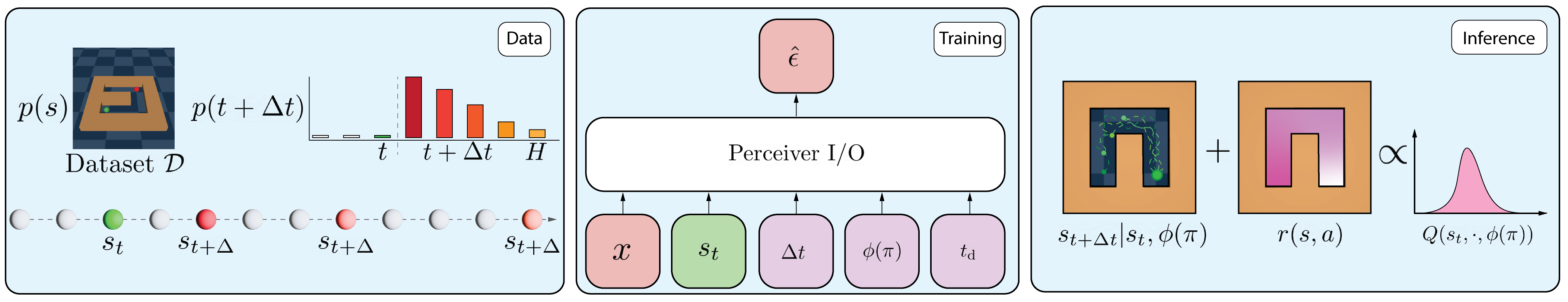
In this paper, we show how we can estimate the environment dynamics in an efficient way while avoiding the dependence of model-based rollouts on the episode horizon. The model learned by our method (1) does not require predicting high-dimensional observations at every timestep, (2) directly predicts the future state without the need of autoregressive unrolls and (3) can be used to estimate the value function without requiring expensive rollouts or temporal difference learning, nor does it need action or reward labels during the pre-training phase. Precisely, we learn a generative model of the discounted state occupancy measure, i.e. a function which takes in a state, action and timestep, and returns a future state proportional to the likelihood of visiting that future state under some fixed policy. This occupancy measure has a resemblance to successor features [14], and can be seen as its generative, normalized version. By scoring these future states by the corresponding rewards, we form an unbiased estimate of the value function. We name our proposed algorithm Diffused Value Function (DVF). Because DVF represents multi-step transitions implicitly, it avoids having to predict high-dimensional observations at every timestep and thus scales to long-horizon tasks with high-dimensional observations. Using the same algorithm, we can handle settings where reward-free and action-free data is provided, which cannot be directly handled by classical TD-based methods. Specifically, the generative model can be pre-trained on sequences of states without the need for reward or action labels, provided that some representation of the data generating process (i.e., logging policy) is known.
We highlight the strengths of DVF both qualitatively and quantitatively on challenging robotic tasks, and show how generative models can be used to accelerate tabula rasa learning.
2 Preliminaries
Reinforcement learning
Let be a Markov decision process (MDP) defined by the tuple , where is a state space, is the set of starting states, is an action space, is a one-step transition function111 denotes the entire set of distributions over the space ., is a reward function and is a discount factor. The system starts in one of the initial states . At every timestep , the policy samples an action . The environment transitions into a next state and emits a reward . The aim is to learn a Markovian policy that maximizes the return, defined as discounted sum of rewards, over an episode of length :
| (1) |
where denotes the joint distribution of obtained by rolling-out in the environment for timesteps starting at timestep . To solve Eq. 1, value-based RL algorithms estimate the future expected discounted sum of rewards, known as the value function:
| (2) |
for , and . Alternatively, the value function can be written as the expectation of the reward over the discounted occupancy measure:
| (3) |
where and as defined in [15].
Diffusion models
Diffusion models form a class of latent variable models [17] which represent the distribution of the data as an iterative process:
| (4) |
for latents with conditional distributions parameterized by . The joint distribution of data and latents factorizes into a Markov Chain with parameters
| (5) |
which is called the reverse process. The posterior , called the forward process, typically takes the form of a Markov Chain with progressively increasing Gaussian noise parameterized by variance schedule :
| (6) |
where can be either learned or fixed as hyperparameter. The parameters of the reverse process are found by minimizing the variational upper-bound on the negative log-likelihood of the data:
| (7) |
Later works, such as Denoising Diffusion Probabilistic Models [DDPM, 18] make specific assumptions regarding the form of , leading to the following simplified loss with modified variance scale :
| (8) |
by training a denoising network to predict noise from a corrupted version of at timestep . Samples from can be generated by following the reverse process:
| (9) |
3 Methodology
Through the lens of Eq. 3, the value function can be decomposed into three components: (1) occupancy measure , dependent on states and policy, (2) reward model dependent on states and actions and (3) policy representation , dependent on the policy. Equipped with these components, we could estimate the value of any given policy in a zero-shot manner. However, two major issues arise:
-
•
For offline222Online training can use implicit conditioning by re-collecting data with the current policy training, has to be explicitly conditioned on the target policy, via the policy representation .
-
•
Maximizing directly as opposed to indirectly via is too costly due to the large size of diffusion denoising networks.
If both challenges are mitigated, then the value function can be estimated by first sampling a collection of states from the learned diffusion model and then evaluating the reward predictor at those states . A similar result can be derived for the state-action value function by training a state-action conditionned diffusion model , from which a policy can be decoded using e.g. the information projection method such as in [20].
3.1 Challenge 1: Off-policy evaluation through conditioning
Explicit policy conditioning has (and still remains) a hard task for reinforcement learning settings. Assuming that the policy has a lossless finite-dimensional representation , passing it to an ideal value function network as could allow for zero-shot policy evaluation. That is, given two policy sets , training on and then swapping out for where would immediately give the estimate of .
We address this issue by studying sufficient statistics of . Since the policy is a conditional distribution, it is possible to use a kernel embedding for conditional distributions such as a Reproducing Kernel Hilbert Space [21, 22], albeit it is ill-suited for high-dimensional non-stationary problems. Recent works have studied using the trajectories as a sufficient statistic for evaluated a key states [23]. Similarly, we studied two policy representations:
-
1.
Scalar: Given a countable policy set indexed by , we let . One example of such sets is the value improvement path, i.e. the number of training gradient steps performed since initialization.
-
2.
Sequential: Inspired by [21], we embed using its rollouts in the environment . In the case where actions are unknown, then the sequence of states can be sufficient, under some mild assumptions333One such case is MDPs with deterministic dynamics, as it allows to figure out the corresponding action sequence., for recovering .
Both representations have their own advantages: scalar representations are compact and introduce an ordering into the policy set , while sequential representations can handle cases where no natural ordering is present in (e.g. learning from offline data).
3.2 Challenge 2. Maximizing the value with large models
In domains with continuous actions, the policy is usually decoded using the information projection onto the value function estimate (see [20]) by minimizing
| (10) |
However, (a) estimating requires estimation of which cannot be pre-trained on videos (i.e. state sequences) and (b) requires the differentiation of the sampling operator from the network, which, in our work, is parameterized by a large generative model. The same problem arises in both model-free [20] and model-based methods [24], where the networks are sufficiently small that the overhead is minimal. In our work, we circumvent the computational overhead by unrolling one step of Bellman backup
| (11) |
and consequently
| (12) |
allowing to learn instead of and using it to construct the state value function.
3.3 Practical algorithm
As an alternative to classical TD learning, we propose to separately estimate the occupancy measure , using a denoising diffusion model and the reward , using a simple regression in symlog space [24]. While it is hard to estimate the occupancy measure directly, we instead learn a denoising diffusion probabilistic model [DDPM, 18], which we call the de-noising network. Since we know what the true forward process looks like at timestep , the de-noising network is trained to predict the input noise.
The high-level idea behind the algorithm is as follows:
-
1.
Pre-train a diffusion model on sequences of states and, optionally, policy embeddings . This step can be performed on large amounts of demonstration videos without the need of any action nor reward labels. The policy embedding can be chosen to be any auxiliary information which allows the model to distinguish between policies444In MDPs with deterministic transitions, one such example is .. This step yields .
-
2.
Using labeled samples, train a reward predictor . This reward predictor will be used as importance weight to score each state-action pair generated by the diffusion model.
-
3.
Sample a state from and score it using , thus obtaining an estimate proportional to the value function of policy at state .
-
4.
Optionally: Maximize the resulting value function estimator using the information projection of onto the polytope of value functions (see Eq. 10) and decoding a new policy . If in the online setting, use to collect new data in the environment and update to .
Algorithm 1 describes the exact training mechanism, which first learns a diffusion model and maximizes its reward-weighted expectation to learn a policy suitable for control. Note that the method is suitable for both online and offline reinforcement learning tasks, albeit conditioning on the policy representation has to be done explicitly in the case of offline RL.
DVF can also be shown to learn an occupancy measure which corresponds to the normalized successor features [14] that allows sampling future states through the reverse diffusion process.
4 Experiments
4.1 Mountain Car
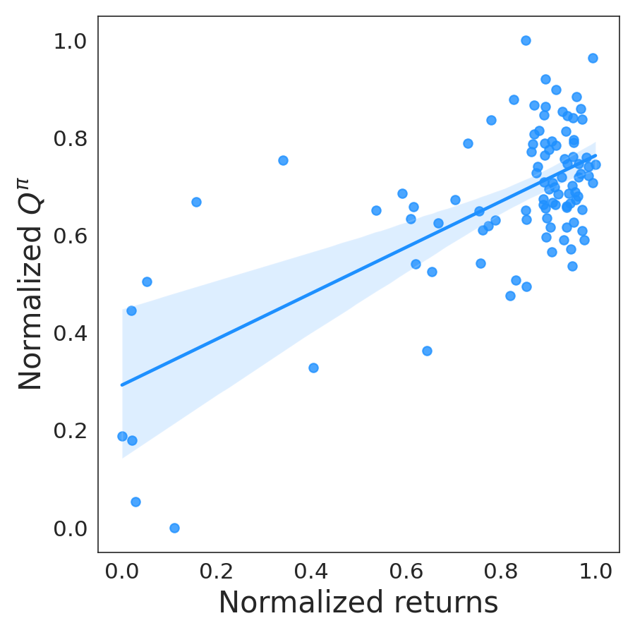
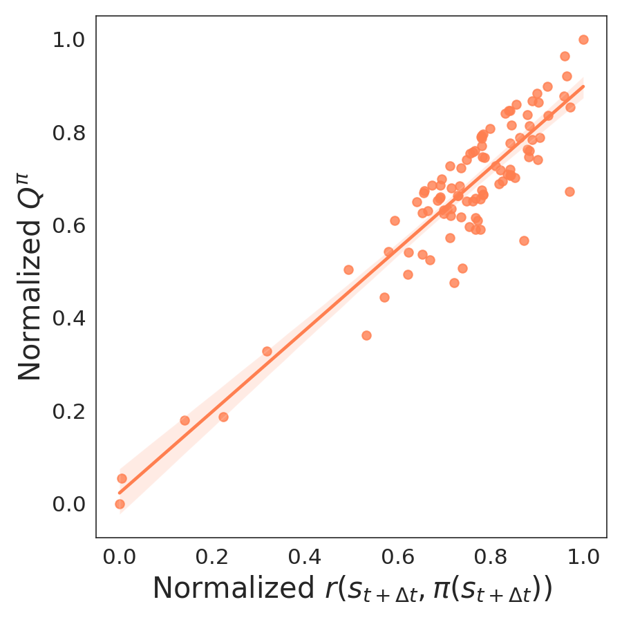
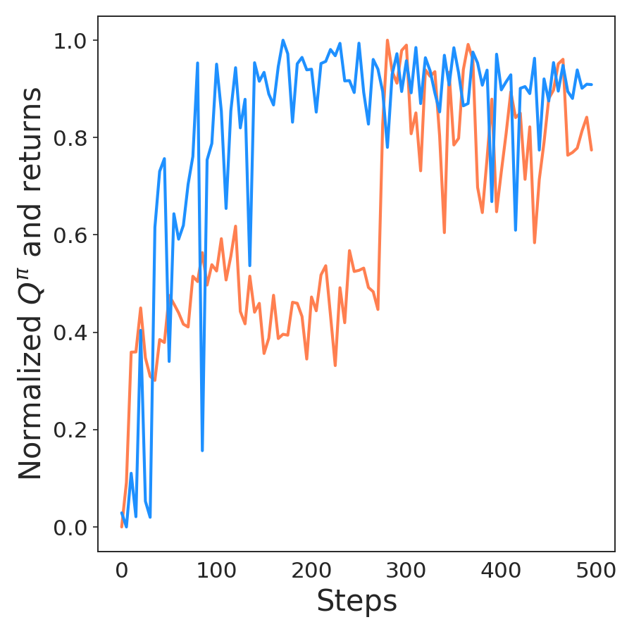
Before studying the behavior of DVF on robotic tasks, we conduct experiments on the continuous Mountain Car problem, a simple domain for analysing sequential decision making methods. We trained DVF for 500 gradient steps until convergence, and computed correlations between the true environment returns, the value function estimator based on the diffusion model, as well as the reward prediction at states sampled from . Fig. 2 shows that all three quantities exhibit strong positive correlation, even though the value function estimator is not learned using temporal difference learning.
4.2 Maze 2d
We examine the qualitative behavior of the diffusion model of DVF on a simple locomotion task inside mazes of various shapes, as introduced in the D4RL offline suite [25]. In these experiments, the agent starts in the lower left of the maze and uses a waypoint planner with three separate goals to collect data in the environment (see Fig. 3(a) and Fig. 3(c) for the samples of the collected data). The diffusion model of DVF is trained on the data from the three data-collecting policies, using the scalar policy conditioning described in Section 3.1.
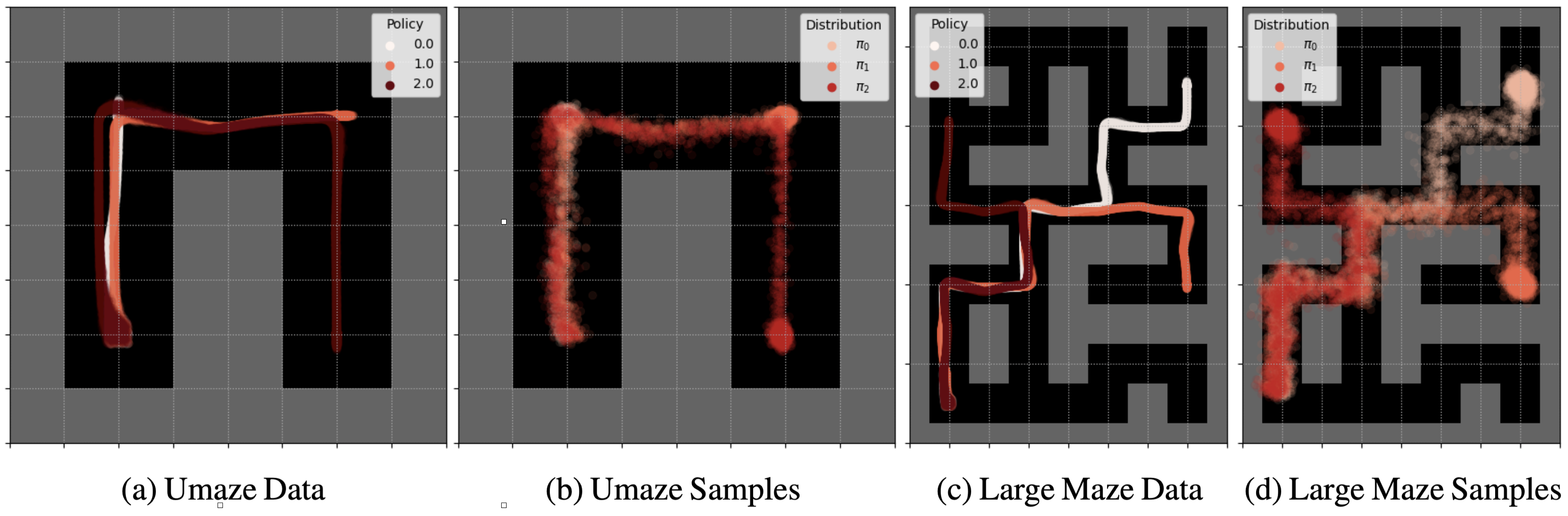
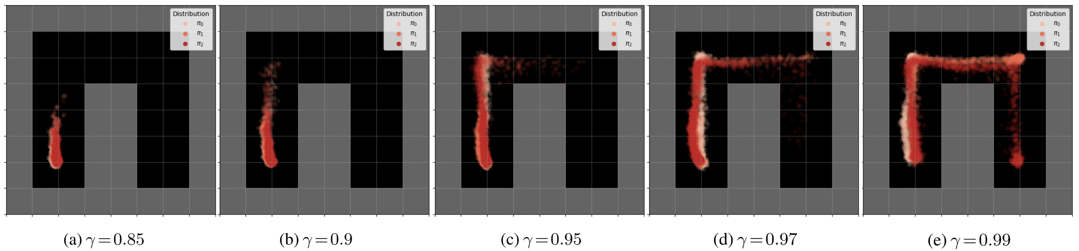
Fig. 3 shows full trajectories sampled by conditioning the diffusion model on the start state in the lower left, the policy index, and a time offset. Fig. 4 shows sampled trajectories as the discount factor increases, leading to sampling larger time offsets.
The results show the ability of the diffusion model to represent long-horizon data faithfully, and highlight some benefits of the approach. DVF can sample trajectories without the need to evaluate a policy or specify intermediate actions. Because DVF samples each time offset independently, there is also no concern of compounding model error as the horizon increases. Additionally, the cost of predicting from is for DVF, while it is for classical autoregressive models.
4.3 PyBullet
Our final set of experiments consists in ablations performed on offline data collected from classical PyBullet environments555Data is taken from https://github.com/takuseno/d4rl-pybullet/tree/master, as oppposed to D4RL, which has faced criticism due to poor sim2real transfer capabilities [26]. We compare DVF to behavior cloning and Conservative Q-learning [27], two strong offline RL baselines. We also plot the average normalized returns of each dataset to facilitate the comparison over 5 random seeds. Medium dataset contains data collected by medium-level policy and mixed contains data from SAC [20] training.
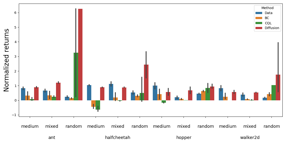
Fig. 5 highlights the ability of DVF to match and sometimes outperform the performance of classical offline RL algorithms, especially on data of lower quality, e.g. coming from a random policy. In domains where online rollouts can be prohibitively expensive, the ability to learn from low-quality, incomplete offline demonstrations is a strength of DVF. This benchmark also demonstrates the shortcomings of scalar policy representation, which is unknown for a given offline dataset, and also doesn’t scale well when the number of policies is large (e.g. number of gradient steps in logging policy ). For this reason, we opted for a sequential policy representation.
5 Related works
Offline pre-training for reinforcement learning
Multiple approaches have tried to alleviate the heavy cost of training agents tabula rasa by pre-training some parts of the system offline. For example, inverse dynamics models which predict the action leading from the current state to the next state have seen success in complex domains such as Atari [28], as well as Minecraft [8, 9]. Return-conditioned sequence models have also seen a rise in popularity, specifically due to their ability to learn performance-action-state correlations over long horizons [29].
Unsupervised reinforcement learning
Using temporal difference [30] for policy iteration or evaluation requires all data tuples to contain state, action and reward information. However, in some real-world scenarios, the reward might only be available for a small subset of data (e.g. problems with delayed feedback [31]). In this case, it is possible to decompose the value function into a reward-dependent and dynamics components, as was first suggested in the successor representation framework [14, 16]. More recent approaches [15, 32, 33, 34] use a density model to learn the occupancy measure over future states for each state-action pair in the dataset. However, learning an explicit multi-step model such as [15] can be unstable due to the bootstrapping term in the temporal difference loss, and these approaches still require large amounts of reward and action labels. While our proposed method is a hybrid between model-free and model-based learning, it avoids the computational overhead incurred by classical world models such as Dreamer [24] by introducing constant-time rollouts. The main issue with infinite-horizon models is the implicit dependence of the model on the policy, which imposes an upper-bound on the magnitude of the policy improvement step achievable in the offline case. Our work solves this issue by adding an explicit policy conditioning mechanism, which allows to generate future states from unseen policy embeddings.
Diffusion models
Learning a conditional probability distribution over a highly complex space can be a challenging task, which is why it is often easier to instead approximate it using a density ratio specified by an inner product in a much lower-dimensional latent space. To learn an occupancy measure over future states without passing via the temporal difference route, one can use denoising diffusion models to approximate the corresponding future state density under a given policy. Diffusion has previously been used in the static unsupervised setting such as image generation [18] and text-to-image generation [35]. Diffusion models have also been used to model trajectory data for planning in small-dimensional environments [36]. However, no work so far has managed to efficiently predict infinite-horizon rollouts.
6 Discussion
In this work, we introduced a simple model-free algorithm for learning reward-maximizing policies, which can be efficiently used to solve complex robotic tasks. Diffused Value Function (DVF) avoids the pitfalls of both temporal difference learning and autoregressive model-based methods by pre-training an infinite-horizon transition model from state sequences using a diffusion model. This model does not require any action nor reward information, and can then be used to construct the state-action value function, from which one can decode the optimal action. DVF fully leverages the power of diffusion models to generate states far ahead into the future without intermediate predictions. Our experiments demonstrate that DVF matches and sometimes outperforms strong offline RL baselines on realistic robotic tasks based on PyBullet, and opens an entire new direction of research.
7 Limitations
The main limitation of our method is that it operates directly on observations instead of latent state embeddings, which requires tuning the noise schedule for each set of tasks, instead of using a unified noise schedule similarly to latent diffusion models [37]. Another limitation is the need to explicitly condition the rollouts from the diffusion model on the policy, something that single-step models avoid. Finally, online learning introduces the challenge of capturing the non-stationarity of the environment using the generative model , which, in itself, is a hard task.
References
- Chowdhery et al. [2022] A. Chowdhery, S. Narang, J. Devlin, M. Bosma, G. Mishra, A. Roberts, P. Barham, H. W. Chung, C. Sutton, S. Gehrmann, et al. Palm: Scaling language modeling with pathways. arXiv preprint arXiv:2204.02311, 2022.
- Touvron et al. [2023] H. Touvron, T. Lavril, G. Izacard, X. Martinet, M.-A. Lachaux, T. Lacroix, B. Rozière, N. Goyal, E. Hambro, F. Azhar, et al. Llama: Open and efficient foundation language models. arXiv preprint arXiv:2302.13971, 2023.
- Kaplan et al. [2020] J. Kaplan, S. McCandlish, T. Henighan, T. B. Brown, B. Chess, R. Child, S. Gray, A. Radford, J. Wu, and D. Amodei. Scaling laws for neural language models. arXiv preprint arXiv:2001.08361, 2020.
- Ouyang et al. [2022] L. Ouyang, J. Wu, X. Jiang, D. Almeida, C. Wainwright, P. Mishkin, C. Zhang, S. Agarwal, K. Slama, A. Ray, et al. Training language models to follow instructions with human feedback. Advances in Neural Information Processing Systems, 35:27730–27744, 2022.
- Brohan et al. [2023] A. Brohan, Y. Chebotar, C. Finn, K. Hausman, A. Herzog, D. Ho, J. Ibarz, A. Irpan, E. Jang, R. Julian, et al. Do as i can, not as i say: Grounding language in robotic affordances. In Conference on Robot Learning, pages 287–318. PMLR, 2023.
- Stone et al. [2023] A. Stone, T. Xiao, Y. Lu, K. Gopalakrishnan, K.-H. Lee, Q. Vuong, P. Wohlhart, B. Zitkovich, F. Xia, C. Finn, et al. Open-world object manipulation using pre-trained vision-language models. arXiv preprint arXiv:2303.00905, 2023.
- Driess et al. [2023] D. Driess, F. Xia, M. S. Sajjadi, C. Lynch, A. Chowdhery, B. Ichter, A. Wahid, J. Tompson, Q. Vuong, T. Yu, et al. Palm-e: An embodied multimodal language model. arXiv preprint arXiv:2303.03378, 2023.
- Baker et al. [2022] B. Baker, I. Akkaya, P. Zhokov, J. Huizinga, J. Tang, A. Ecoffet, B. Houghton, R. Sampedro, and J. Clune. Video pretraining (vpt): Learning to act by watching unlabeled online videos. Advances in Neural Information Processing Systems, 35:24639–24654, 2022.
- Fan et al. [2022] L. Fan, G. Wang, Y. Jiang, A. Mandlekar, Y. Yang, H. Zhu, A. Tang, D.-A. Huang, Y. Zhu, and A. Anandkumar. Minedojo: Building open-ended embodied agents with internet-scale knowledge. arXiv preprint arXiv:2206.08853, 2022.
- Yu et al. [2020] T. Yu, G. Thomas, L. Yu, S. Ermon, J. Y. Zou, S. Levine, C. Finn, and T. Ma. Mopo: Model-based offline policy optimization. Advances in Neural Information Processing Systems, 33:14129–14142, 2020.
- Argenson and Dulac-Arnold [2020] A. Argenson and G. Dulac-Arnold. Model-based offline planning. arXiv preprint arXiv:2008.05556, 2020.
- Kidambi et al. [2020] R. Kidambi, A. Rajeswaran, P. Netrapalli, and T. Joachims. Morel: Model-based offline reinforcement learning. arXiv preprint arXiv:2005.05951, 2020.
- Yu et al. [2021] T. Yu, A. Kumar, R. Rafailov, A. Rajeswaran, S. Levine, and C. Finn. Combo: Conservative offline model-based policy optimization. Advances in neural information processing systems, 34:28954–28967, 2021.
- Dayan [1993] P. Dayan. Improving generalization for temporal difference learning: The successor representation. Neural Computation, 5(4):613–624, 1993.
- Janner et al. [2020] M. Janner, I. Mordatch, and S. Levine. Generative temporal difference learning for infinite-horizon prediction. arXiv preprint arXiv:2010.14496, 2020.
- Barreto et al. [2016] A. Barreto, W. Dabney, R. Munos, J. J. Hunt, T. Schaul, H. Van Hasselt, and D. Silver. Successor features for transfer in reinforcement learning. arXiv preprint arXiv:1606.05312, 2016.
- Sohl-Dickstein et al. [2015] J. Sohl-Dickstein, E. Weiss, N. Maheswaranathan, and S. Ganguli. Deep unsupervised learning using nonequilibrium thermodynamics. In International Conference on Machine Learning, pages 2256–2265. PMLR, 2015.
- Ho et al. [2020] J. Ho, A. Jain, and P. Abbeel. Denoising diffusion probabilistic models. Advances in Neural Information Processing Systems, 33:6840–6851, 2020.
- Jaegle et al. [2021] A. Jaegle, S. Borgeaud, J.-B. Alayrac, C. Doersch, C. Ionescu, D. Ding, S. Koppula, D. Zoran, A. Brock, E. Shelhamer, et al. Perceiver io: A general architecture for structured inputs & outputs. arXiv preprint arXiv:2107.14795, 2021.
- Haarnoja et al. [2018] T. Haarnoja, A. Zhou, P. Abbeel, and S. Levine. Soft actor-critic: Off-policy maximum entropy deep reinforcement learning with a stochastic actor. In International conference on machine learning, pages 1861–1870. PMLR, 2018.
- Song et al. [2013] L. Song, K. Fukumizu, and A. Gretton. Kernel embeddings of conditional distributions: A unified kernel framework for nonparametric inference in graphical models. IEEE Signal Processing Magazine, 30(4):98–111, 2013.
- Mazoure et al. [2022] B. Mazoure, T. Doan, T. Li, V. Makarenkov, J. Pineau, D. Precup, and G. Rabusseau. Low-rank representation of reinforcement learning policies. Journal of Artificial Intelligence Research, 75:597–636, 2022.
- Harb et al. [2020] J. Harb, T. Schaul, D. Precup, and P.-L. Bacon. Policy evaluation networks. arXiv preprint arXiv:2002.11833, 2020.
- Hafner et al. [2023] D. Hafner, J. Pasukonis, J. Ba, and T. Lillicrap. Mastering diverse domains through world models. arXiv preprint arXiv:2301.04104, 2023.
- Fu et al. [2020] J. Fu, A. Kumar, O. Nachum, G. Tucker, and S. Levine. D4rl: Datasets for deep data-driven reinforcement learning, 2020.
- Körber et al. [2021] M. Körber, J. Lange, S. Rediske, S. Steinmann, and R. Glück. Comparing popular simulation environments in the scope of robotics and reinforcement learning. arXiv preprint arXiv:2103.04616, 2021.
- Kumar et al. [2020] A. Kumar, A. Zhou, G. Tucker, and S. Levine. Conservative q-learning for offline reinforcement learning. arXiv preprint arXiv:2006.04779, 2020.
- Schwarzer et al. [2021] M. Schwarzer, N. Rajkumar, M. Noukhovitch, A. Anand, L. Charlin, D. Hjelm, P. Bachman, and A. Courville. Pretraining representations for data-efficient reinforcement learning. arXiv preprint arXiv:2106.04799, 2021.
- Lee et al. [2022] K.-H. Lee, O. Nachum, M. S. Yang, L. Lee, D. Freeman, S. Guadarrama, I. Fischer, W. Xu, E. Jang, H. Michalewski, et al. Multi-game decision transformers. Advances in Neural Information Processing Systems, 35:27921–27936, 2022.
- Sutton and Barto [2018] R. S. Sutton and A. G. Barto. Reinforcement learning: An introduction. MIT press, 2018.
- Howson et al. [2021] B. Howson, C. Pike-Burke, and S. Filippi. Delayed feedback in episodic reinforcement learning. arXiv preprint arXiv:2111.07615, 2021.
- Eysenbach et al. [2020] B. Eysenbach, R. Salakhutdinov, and S. Levine. C-learning: Learning to achieve goals via recursive classification. arXiv preprint arXiv:2011.08909, 2020.
- Eysenbach et al. [2022] B. Eysenbach, T. Zhang, R. Salakhutdinov, and S. Levine. Contrastive learning as goal-conditioned reinforcement learning. arXiv preprint arXiv:2206.07568, 2022.
- Mazoure et al. [2022] B. Mazoure, B. Eysenbach, O. Nachum, and J. Tompson. Contrastive value learning: Implicit models for simple offline rl, 2022.
- Rombach et al. [2022] R. Rombach, A. Blattmann, D. Lorenz, P. Esser, and B. Ommer. High-resolution image synthesis with latent diffusion models. In Proceedings of the IEEE/CVF Conference on Computer Vision and Pattern Recognition, pages 10684–10695, 2022.
- Janner et al. [2022] M. Janner, Y. Du, J. B. Tenenbaum, and S. Levine. Planning with diffusion for flexible behavior synthesis. arXiv preprint arXiv:2205.09991, 2022.
- Rombach et al. [2022] R. Rombach, A. Blattmann, D. Lorenz, P. Esser, and B. Ommer. High-resolution image synthesis with latent diffusion models. In Proceedings of the IEEE/CVF Conference on Computer Vision and Pattern Recognition (CVPR), pages 10684–10695, June 2022.
Appendix
7.1 Experimental details
Model architecture
DVF uses a Perceiver I/O model [19] with convolution encodings for states, sinusoidal encoding for diffusion timestep and a linear layer for action embedding. The Perceiver I/O model has positional encodings for all inputs, followed by 8 blocks with 4 cross-attention heads and 4 self-attention heads and latent size 256. The scalar policy representation was encoded using sinusoidal encoding, while the sequential representation was passed through the convolution and linear embedding layers and masked-out to handle varying context lengths, before being passed to the Perceiver model.
| Hyperparameter | Value |
|---|---|
| Learning rate | |
| Batch size | |
| Discount factor | 0.99 |
| Max gradient norm | 100 |
| MLP structure | DenseNet MLP |
| Add LayerNorm in between all layers | Yes |
| Hyperparameter | Value |
|---|---|
| DVF | |
| Number of future state samples | 32 |
| BC coefficient | 0.1 (offline) and 0 (online) |
| CQL | |
| Regularization coefficient | 1 |
All experiments were run on the equivalent of 2 V100 GPUs with 32 Gb of VRAM and 8 CPUs.
Dataset composition
The Maze2d datasets were constructed based on waypoint planning scripts provided in the D4RL repository, and modifying the target goal locations to lie in each corner of the maze (u-maze), or in randomly chosen pathways (large maze). The PyBullet dataset has a data composition similar to the original D4RL suite, albeit collected in the PyBullet simulator instead of MuJoCo.
7.2 Additional results
We include three videos of the training of the diffusion model on the large maze dataset shown in Fig. 4 for 128, 512 and 1024 diffusion timesteps, in the supplementary material. Note that increasing the number of timesteps leads to faster convergence of the diffusion model samples to the true data distribution.