Simulation of ab initio optical absorption spectrum of $\beta$-carotene with fully resolved $S_{0}$ and $S_{2}$ vibrational normal modes

Abstract

Electronic absorption spectrum of $\beta$-carotene ($\beta$-Car) is studied using quantum chemistry and quantum dynamics simulations. Vibrational normal modes were computed in optimized geometries of the electronic ground state $S_{0}$ and the optically bright excited $S_{2}$ state using the time-dependent density functional theory. By expressing the $S_{2}$ state normal modes in terms of the ground state modes, we find that no one-to-one correspondence between the ground and excited state vibrational modes exists. Using the ab initio results, we simulated $\beta$-Car absorption spectrum with all 282 vibrational modes in a model solvent at $300\ \text{K}$ using the time-dependent Dirac-Frenkel variational principle (TDVP) and are able to qualitatively reproduce the full absorption lineshape. By comparing the 282-mode model with the prominent 2-mode model, widely used to interpret carotenoid experiments, we find that the full 282-mode model better describe the high frequency progression of carotenoid absorption spectra, hence, vibrational modes become highly mixed during the $S_{0}\rightarrow S_{2}$ optical excitation. The obtained results suggest that electronic energy dissipation is mediated by numerous vibrational modes.

1 Introduction

Pigment molecules in Nature form the basis of life on Earth by enabling organisms to utilize the solar energy. Carotenoids form a unique class of pigments with a conjugated polyene chain, responsible for light absorption in green-blue color region. Over 700 carotenoid molecules are found in Nature. They primarily play a role as coloring materials, what underlie a vital and complex signalling processes ¹, ². In photosynthesis carotenoids are essential in solar energy harvesting and in photoprotection from oxygen damage. The latter emerge on microscopic level, when light illumination is high, by formation of energy trapping states ³, ⁴. This trapping has been related to quenching of the chlorophyll excited states by carotenoid singlet state ⁵, ⁶, or by excitonic interaction between chlorophyll and the carotenoid which is controlled by carotenoid conformations ⁷, ⁸. Carotenoids become thus responsible for regulation of excitation energy fluxes in photosynthesis in volatile conditions of daylight irradiation. One of the possible mechanisms of such behavior involves a limited conformational rearrangement of the protein scaffold, that could act as a molecular switch to activate or deactivate the quenching mechanism ⁹. A strong correlation between carotenoid and local environment deformations is necessary for such mechanism to exist.

However, the primary deformations leading to carotenoid flexibility are the molecular vibrations. They are usually induced during photon absorption (and emission) and following excitation relaxation processes. Probing excitation and vibration mediated relaxation processes in carotenoids, necessary for understanding fundamental physical processes involved in their functioning, is possible by performing time-resolved optical spectroscopy experiments. It is well established that carotenoids demonstrate a complex structure of electronic excited states ¹⁰, ¹¹ with at least three electronic states necessary to fully capture excitation long-time dynamics. Direct optical excitation induces electronic $S_{0}\rightarrow S_{2}$ transition, where $S_{0}$ is the electronic ground state and $S_{2}$ is the first optically accessible (bright) electronic state, and the optically dark electronic state $S_{1}$ lies between $S_{0}$ and $S_{2}$. Additional intramolecular charge-transfer (CT) states have been proposed in peridinin in agreement with the experimental results ¹², ¹³. Quantum chemical calculations using the time-dependent density functional theory with the Tamm−Dancoff approximation ¹⁴, ¹⁵, ¹⁶ demonstrate presence of CT state, which appears as the third and second excited singlet state, respectively. Energy of the CT state has been shown to decrease dramatically in solvents of increasing polarity, while the energy of the dark $S_{1}$ state remains comparatively constant ¹⁷. Several other types of electronic excited states have been suggested, however, their existence and involvement in relaxation process is still debatable ¹⁸. Specific spectral features have been assigned to $S_{1}$ and CT states and these may play an important role in deexcitation processes ¹³, ¹⁹, ⁹.

Vibrational heating and cooling is involved in the relaxation process via the electonic-vibrational (vibronic) coupling ²⁰. Indeed, the strong vibronic coupling is rooted in a broad electronic absorption spectra, more specifically, in a strong vibronic shoulder for a range of different carotenoids as observed experimentally ²¹. This feature is often associated with two vibrational modes: C-C symmetric and asymmetric stretching vibrations with cumulative Huang-Rhys factor larger than 1. These modes are known to be active in Raman spectra and their frequencies scale linearly with the conjugation length in carotenoids ¹¹. While molecular vibrations affect symmetry properties of molecules, they do not affect the oscillator strength of the dark state ²². Such empirical effective 2-mode model has been extensively used for spectroscopy simulations ²³, ²⁴, ²⁵, ²⁶, ²⁷, ²⁰. However, the two vibrational modes do not capture the high energy vibrational wing and it is not clear whether the two modes are sufficient to accurately describe the more complex ultrafast internal conversion and energy transfer processes.

In this paper we present quantum chemistry and quantum dynamics description of vibrational manifold of $\beta$-Car in its electronic states $S_{0}$ and $S_{2}$. We find that numerous vibrational modes become highly mixed during the $S_{0}\rightarrow S_{2}$ optical excitation, resulting in a complex $S_{2}$ state wavepacket. We are able to reveal the full absorption spectrum, including the high-energy vibrational shoulder, however, qualitatively correct vibrational peak ratios require the raw quantum chemistry results to be scaled. Simulations thus suggest that pathways responsible for the ultrafast electronic excitation relaxation and internal conversion are mediated by numerous vibrational modes resulting in a rapid and efficient electronic energy dissipation.

2 Theoretical Methods

Quantum chemical analysis starts from the complete molecular Hamiltonian including both electronic and vibrational degrees of freedom (DOFs) ²⁸, ²⁹. Using the Born-Oppenheimer approximation the full Schrödinger equation is split into separate equations for electronic and nuclear DOFs. The stationary Schrödinger equation for electrons then parametrically depends on the nuclear coordinates

$$\hat{H}_{el}(\boldsymbol{R})\Phi_{m}(\boldsymbol{R})=E_{m}(\boldsymbol{R})\Phi_{m}(\boldsymbol{R}).$$ (1)

Here $\hat{H}_{el}$ includes electron kinetic energy, electronic interaction with nuclei, electron-electron interactions and internuclear interaction energy, $\boldsymbol{R}\equiv R_{1},R_{2}...$ labels nuclei coordinates. Eigenvalues $E_{m}(\boldsymbol{R})$ and the corresponding eigenstates $\Phi_{m}(\boldsymbol{R})$, which parametrically depend on nuclei configuration, characterize electronic system.

Electronic energy minimum of the electronic ground state denotes the reference point - the equilibrium molecular structure. If the nuclear configuration deviates from the minimum, the electronic energy is increased, hence, the electronic energy can be treated as the potential energy for nuclei DOFs. For small deviations from the energy minimum, we use the harmonic approximation, where the potential energy operator is expanded up to quadratic terms. So, the potential energy for nuclei displacements in electronic state $n$ can be written as (using Einstein summation convention for repeating indices)

$$U_{n}(\boldsymbol{u})\approx\frac{1}{2}\mathcal{H}_{ij}^{(n)}u_{i}u_{j},$$ (2)

where we introduce mass-weighted Cartesian coordinates $u_{i}=\sqrt{M_{i}}\left(R_{i}-R_{i0}^{n}\right)$, as the shifts of nuclei from their equilibrium positions, and

$$\mathcal{H}_{ij}^{(n)}=\frac{1}{\sqrt{M_{i}M_{j}}}\left.\frac{\partial^{2}E_{n}(\boldsymbol{R})}{\partial R_{i}\partial R_{j}}\right|_{\text{min}},$$ (3)

is the Hessian matrix with derivatives taken at the global minimum of the state $n$. Schrödinger equation for the nuclear wavefunctions with respect to the specific electronic state $n$ is

$$\left(\hat{T}+\hat{U}_{n}(\boldsymbol{u})\right)\chi_{n\alpha}(\boldsymbol{u})=\varepsilon_{n\alpha}\chi_{n\alpha}(\boldsymbol{u}).$$ (4)

Here $\alpha$ is the vibrational quantum state index with energy $\varepsilon_{n\alpha}$ and wavefunction $\chi_{\alpha n}$. Vibrational Schrödinger equation splits into independent set of equations in the normal coordinate representation; we denote these coordinates by $Q_{k}$. Normal modes are obtained by diagonalizing the Hessian matrix for each electronic state $n$. Solving the eigenstate equation

$$\mathcal{H}_{ij}^{(n)}L_{jk}^{(n)}=\omega_{nk}^{2}L_{ik}^{(n)},$$ (5)

yields normal mode frequencies $\omega_{nk}$, where $k$ labels normal modes. The Hessian eigenvectors $L_{ik}^{(n)}$ relate normal modes $k$ and nuclei displacements $u_{i}$. Placing eigenvectors in columns, we form the matrix $L^{(n)}$, whose rank is $M=3N-6$ (six of the modes are physically irrelevant as 3 of them correspond to the uniform translation of the whole molecule along Cartesian axes, while the other 3 are uniform rotations about these axes, they are excluded), and it is used to transform mass-weighted Cartesian internal coordinates $u_{i}$ into normal coordinates $Q_{k}^{(n)}=\left(L^{(n)}\right)_{kl}^{-1}u_{l}$.

Complete description of the vibronic molecular states, when electronic and vibrational state is known, is given by the state vectors $|n\bm{\alpha}_{n}\rangle$, where $\bm{\alpha}_{n}$$\equiv(\alpha_{n1},\alpha_{n2},...,\alpha_{nK})$ is the $M-$dimensional vector denoting vibrational states of all vibrational modes in electronic state $n$. As normal modes are harmonic, vibrational Hamiltonian in electronic state $n$ is given by

$$\hat{H}^{(n)}=\frac{1}{2}\sum_{k}\left(\left(\hat{P}_{k}^{(n)}\right)^{2}+\omega_{nk}^{2}\left(\hat{Q}_{k}^{(n)}\right)^{2}\right)|n\rangle\langle n|.$$ (6)

Absorption spectrum of a vibronic system involves all possible optical transitions from the vibronic ground state $|g\bm{\beta}\rangle$ to the excited states $|e\bm{\alpha}\rangle$. Starting from the linear response theory, the absorption spectrum is given by the Fourier transform of the linear response function

$$S(\omega)=\frac{\omega}{nc}\text{Re}\int_{0}^{\infty}\text{d}te^{i\omega t}F\left(t\right),$$ (7)

where n is the refraction index and c is the speed of light ³⁰, ²⁸, and

$$F\left(t\right)=\langle g\bm{\alpha}|e^{i\hat{H}_{g}t}\hat{\bm{P}}e^{-i\hat{H}_{e}t}\hat{\bm{P}}|g\bm{\alpha}\rangle,$$ (8)

is the dipole operator correlation function. In the Born approximation the polarization operator $\hat{\bm{P}}$ acts only on electronic DOFs, hence, $\hat{\boldsymbol{P}}=\bm{\mu}_{eg}^{(el)}\left(|e\rangle\langle g|+|g\rangle\langle e|\right)$ and $\bm{\mu}_{eg}^{(el)}$ is the electronic transition dipole. Matrix elements of the polarization operator are given by

$$\langle e\bm{\alpha}|\hat{\bm{P}}|g\bm{\beta}\rangle=\bm{\mu}_{eg}^{(el)}\int\text{d}^{N}\boldsymbol{u}\prod_{j,k}\chi_{e\alpha_{j}}^{\star}(\boldsymbol{u})\chi_{g\beta_{k}}(\boldsymbol{u}).$$ (9)

The multi-dimensional integral correspond to vibrational overlaps between vibrational wavefunction in different electronic states. Integral computation is not trivial, because the sets of normal modes in different electronic states are not orthogonal, transformation of one set of normal modes into another is necessary ³¹, ³², ³³.

Difference of the set of normal modes in different electronic states are characterized as follows. In electronic state $n$ the deviation of atomic Cartesian coordinates $R_{i}$ from the equilibrium position $R_{i0}^{(n)}$ may be expressed via the normal modes via relation

$$\sqrt{M_{i}}\left(R_{i}-R_{i0}^{(n)}\right)=L_{ij}^{(n)}Q_{j}^{(n)},$$ (10)

and allow us to relate the relative mass-weighted atom shifts $D_{i}^{(mn)}\equiv\sqrt{M_{i}}\left(R_{i0}^{(m)}-R_{i0}^{(n)}\right)$ between the equilibrium positions in electronic states $m$ and $n$ as

$$D_{i}^{(mn)}=L_{ij}^{(n)}Q_{j}^{(n)}-L_{ij}^{(m)}Q_{j}^{(m)}.$$ (11)

Then the normal mode coordinates in state $m$ can be expressed in terms of state $n$ normal mode coordinates as

$$Q_{i}^{(m)}=a_{ij}^{(mn)}Q_{j}^{(n)}-d_{i}^{(mn)},$$ (12)

where the expansion coefficient of the $i$th normal mode in the $m$th state in terms of the $j$th mode in $n$th state is

$$a_{ij}^{(mn)}\equiv\left(L^{(m)}\right)_{ik}^{-1}L_{kj}^{(n)},$$ (13)

and the $i$th normal mode potential displacement in the $m$th state, with respect to the position in the $n$th state, is

$$d_{i}^{(mn)}\equiv\left(L^{(m)}\right)_{ik}^{-1}D_{k}^{(mn)}.$$ (14)

These are the two quantities that relate normal modes in different electronic states. Likewise, normal mode momentum is also expanded in terms of the $a_{kj}^{(eg)}$ coefficients (and zero displacement)

$$P_{i}^{(m)}\equiv a_{ij}^{(mn)}P_{j}^{(n)}.$$ (15)

Further on we consider two electronic states: the ground state $|g\rangle$ and the electronic excited state $|e\rangle$. Instead of evaluating propagators in Eq. (8) by computing the multi-dimensional vibrational overlaps in Eq. (9), we choose to specify a vibronic state basis using the coherent state representation, and propagate it following the TDVP.

We begin with writing dimensionless Hamiltonian by introducing the dimensionless momentum $\hat{p}_{k}^{(n)}\equiv\sqrt{\omega_{nk}}^{-1}\hat{P}_{k}^{(n)}$ and coordinate $\hat{q}_{k}^{(n)}\equiv\sqrt{\omega_{nk}}\hat{Q}_{k}^{(n)}$ operators for $n=g,e$. After inserting them in Eq. (6), follows that the electronic ground state Hamiltonian is

$$\hat{H}^{(g)}=\sum_{k}\frac{\omega_{gk}}{2}\left(\left(\hat{p}_{k}^{(g)}\right)^{2}+\left(\hat{x}_{k}^{(g)}\right)^{2}\right)|g\rangle\langle g|,$$ (16)

and the electronic excited state $|e\rangle$ Hamiltonian is

$$\hat{H}^{(e)} =\left(\varepsilon_{e}+\Lambda_{e}^{\text{vib}}+\sum_{k}\frac{\omega_{ek}}{2}\left(\left(\hat{p}_{k}^{(e)}\right)^{2}+\left(\hat{x}_{k}^{(e)}\right)^{2}\right)\right)|e\rangle\langle e|$$

$$-\sum_{k}\omega_{ek}\tilde{d}_{k}^{(eg)}\hat{x}_{k}^{(e)}|e\rangle\langle e|,$$ (17)

where $\tilde{d}_{k}^{(eg)}\equiv\sqrt{\omega_{ek}}d_{k}^{(eg)}$ is the dimensionless displacement and $\Lambda_{e}^{\text{vib}}\equiv\frac{1}{2}\sum_{k}\omega_{ek}\left(\tilde{d}_{k}^{(eg)}\right)^{2}$ is the total vibrational reorganization energy. The resulting operators in Eqs. (16-17) read

$$\hat{x}_{k}^{(n)}\equiv\beta_{nk,j}a_{kj}^{(ng)}\hat{q}_{j}^{(g)},$$ (18)

$$\hat{p}_{k}^{(n)}\equiv\beta_{nk,j}^{-1}a_{kj}^{(ng)}\hat{p}_{j}^{(g)},$$ (19)

where $\beta_{nk,j}\equiv\sqrt{\omega_{nk}/\omega_{gj}}$. Eq. (18) and (19) describe the dimensionless coordinate and momentum of the $k$th normal mode about its equilibrium point in the $n$th electronic state. Terms $\beta_{nk,j}$ appear due to the normal mode mixing and different vibrational frequencies in state $g$ and $e$. We also add $\varepsilon_{e}$ as the purely electronic excitation energy and set $\varepsilon_{g}=0\ \text{cm}^{-1}$. The total system Hamiltonian is the sum over all electronic state terms $\hat{H}_{S}=\hat{H}^{(g)}+\hat{H}^{(e)}$.

Solvent effects will be simulated by considering energy fluctuations of the molecular environment. Thermal fluctuations are induced by a set of the quantum harmonic oscillators of a given temperature, we will refer to this subsystem as the phonon bath. The phonon bath Hamiltonian is

$$\hat{H}_{\text{B}}=\sum_{p}\frac{w_{p}}{2}\left(\hat{\rho}_{p}^{2}+\hat{\chi}_{p}^{2}\right),$$ (20)

where $w_{p}$ is the frequency of the $p$th phonon mode, while $\hat{\rho}_{p}$ and $\hat{\chi}_{p}$ are the momentum and the coordinate operators, respectively. Interaction between the system electronic states and the phonon bath is included using the displaced oscillator model ²⁹, with the system-bath interaction Hamiltonian

$$\hat{H}_{\text{S-B}}=-\sum_{p}w_{p}f_{ep}\hat{\chi}_{p}|e\rangle\langle e|,$$ (21)

here $f_{ep}$ is the electron-phonon coupling strength of the $p$th phonon mode to the electronic state $e$. The electronic ground state is taken as the reference point so it is not affected by bath fluctuations $f_{gp}=0$. Notice, that the system-bath coupling has the same form as the last term in Eq. (17). The electronic state energy modulation by the intramolecular and intermolecular vibrations is treated equivalently. Likewise, we get additional contribution to the reorganization energy $\Lambda_{e}^{\mathrm{\text{ph}}}=\frac{1}{2}\sum_{p}w_{p}f_{ep}^{2}$. Usually, all excited electronic states are described as having the same coupling strength to the bath, thus, changing all states’ energies by the same amount. For simplicity, we absorb $\Lambda_{e}^{\mathrm{\text{ph}}}$ into the definition of the excited state energy $\varepsilon_{e}$, however, $\Lambda_{e}^{\mathrm{\text{ph}}}$ is still used to define the electron-phonon coupling strengths $f_{ep}$. The full model Hamiltonian is the sum of terms

$$\hat{H}=\hat{H}_{S}+\hat{H}_{\text{B}}+\hat{H}_{\text{S-B}}.$$ (22)

Fluctuation characteristics of the phonon bath can be represented by the spectral density function

$$C_{e}^{"}\left(\omega\right)=\frac{\pi}{2}\sum_{p}f_{ep}^{2}w_{p}^{2}\left[\delta\left(\omega-w_{p}\right)-\delta\left(\omega+w_{p}\right)\right],$$ (23)

where $\delta\left(\omega\right)$ is the Dirac delta function. Integration of Eq. (23) over the complete frequency range defines the phonon bath reorganization energy in the $n$th electronic state

$$\Lambda_{e}^{\text{ph}}=\frac{1}{\pi}\int_{0}^{\infty}\frac{C_{e}^{"}\left(w\right)}{w}\text{d}w=\frac{1}{2}\sum_{p}w_{p}f_{ep}^{2}.$$ (24)

Many theories have been proposed to evaluate the linear response function and the necessary polarization operator matrix elements (Eqs. 8, 9). Notibly, the foundational theory by Yan and Mukamel ³⁴, Franck-Condon approaches ³⁵, ³⁶, ³⁷, as well as, the theories that include include non-Condon effects ³⁸, ³⁹, ⁴⁰, ⁴¹.

We chose to compute the linear response function by propagating the Davydov $\text{D}_{2}$ trial wavefunction originating from the molecular chain soliton theory ⁴², ⁴³. For $N$ electronic states, we can write an arbitrary state of the system as a superposition – the Davydov $\text{D}_{2}$ wavefunction is

$$|\Psi\left(t\right)\rangle =\sum_{n}\alpha_{n}(t)\underbrace{|n\rangle\times|\tilde{\lambda}_{1}\left(t\right),\tilde{\lambda}_{2}\left(t\right),\ldots,\tilde{\lambda}_{K}\left(t\right)\rangle}_{\text{molecule state}}$$

$$\times\underbrace{|\lambda_{1}\left(t\right),\lambda_{2}\left(t\right),\ldots,\lambda_{P}\left(t\right)\rangle}_{\text{solvent phonon state}}.$$ (25)

It utilises coherent state representation for all vibrational modes. For the shifted harmonic oscillator model, coherent states results in an exact dynamics ⁴⁴. $\alpha_{n}\left(t\right)$ is the amplitude of electronic state $|n\rangle$, in our case $n=g,e$. Vibrational and phonon bath modes are represented using coherent states $|\lambda\left(t\right)\rangle=\exp\left(\lambda\left(t\right)\hat{b}^{\dagger}-\lambda^{\star}\left(t\right)\hat{b}\right)|0\rangle$, defined with respect to electronic ground state vibrational modes, where $\lambda\left(t\right)$ is the coherent state parameter, and $|0\rangle$ is the vacuum state of a quantum harmonic oscillator. $\hat{b}_{i}^{\dagger}$ and $\hat{b}_{i}$ are the corresponding bosonic creation and annihilation operators. Only the electronic ground state normal modes are represented by the coherent states, modes of the excited state are expanded in terms of the ground state coherent states. Davydov type wavefunctions have been extensively used to model single molecule, as well as, their aggregate dynamics ⁴⁵, ⁴⁶, ⁴⁷, ⁴⁸, ⁴⁹, linear and nonlinear spetra ⁵⁰, ⁵¹, ⁵², ⁵³, ⁵⁴.

Time evolution of the Davydov $\text{D}_{2}$ wavefunction is obtained by applying the Euler-Lagrange equation

$$\frac{\text{d}}{\text{d}t}\left(\frac{\partial\mathcal{L}\left(t\right)}{\partial\dot{\eta}_{i}^{\star}\left(t\right)}\right)-\frac{\partial\mathcal{L}\left(t\right)}{\partial\eta_{i}^{\star}\left(t\right)}=0,$$ (26)

to each of the time-dependent parameter $\eta_{i}=\alpha_{n},\tilde{\lambda}_{k},\lambda_{p}$, where

$$\mathcal{L}\left(t\right)=\frac{\text{i}}{2}\left(\langle\Psi|\frac{\text{d}}{\text{d}t}\Psi\rangle-\langle\frac{\text{d}}{\text{d}t}\Psi|\Psi\rangle\right)-\langle\Psi|\hat{H}|\Psi\rangle,$$ (27)

is the Lagrangian of the model given in terms of the Hamiltonian $\hat{H}$. For convenience, we ommit explicitly writing time dependence. Euler-Lagrange equation yields a system of coupled differential equations for the $\alpha_{n}$, $\tilde{\lambda}_{k}$, $\lambda_{p}$ parameters of the Davydov $\text{D}_{2}$ wavefunction, see Supplementary Information for the full derivation. Equations describing model dynamics while system is in the excited state $|e\rangle$ are

$$\frac{\text{d}}{\text{d}t}\alpha_{e}= -\text{i}\alpha_{e}\left(\varepsilon_{e}+\Lambda_{e}^{\text{vib}}+\sum_{k,j}\frac{\omega_{ek}^{2}+\omega_{gj}^{2}}{4\omega_{gj}}\left(a_{kj}^{(eg)}\right)^{2}\right)$$

$$+\text{i}\alpha_{e}\left(\sum_{k}\frac{\omega_{ek}}{2}d_{k}^{(eg)}x_{k}^{(e)}+\sum_{q}w_{q}\frac{f_{eq}}{\sqrt{2}}\text{Re}\lambda_{q}\right),$$ (28)

$$\frac{\text{d}}{\text{d}t}\tilde{\lambda}_{k}= -\text{i}\sum_{j}\frac{\omega_{ej}}{\sqrt{2}}\beta_{ej,k}a_{jk}^{(eg)}\left(x_{j}^{(e)}-d_{j}^{(eg)}+\text{i}p_{j}^{(e)}\right),$$ (29)

$$\frac{\text{d}}{\text{d}t}\lambda_{q}= -\text{i}w_{q}\left(\lambda_{q}-\frac{f_{eq}}{\sqrt{2}}\right).$$ (30)

where $x_{k}^{(e)}=\beta_{ek,j}a_{kj}^{(eg)}\sqrt{2}\text{Re}\tilde{\lambda}_{j}$ and $p_{k}^{(e)}=\beta_{ek,j}^{-1}a_{kj}^{(eg)}\sqrt{2}\text{Im}\tilde{\lambda}_{j}$ are the expectation values of operators in Eq. (18) and (19). The resulting system of equations for the ground state $|g\rangle$ dynamics can be solved analytically $\alpha_{g}\left(t\right)=\alpha_{g}\left(0\right)\exp\left(-\frac{\text{i}}{2}\sum_{k}\omega_{gk}t\right)$, $\tilde{\lambda}_{k}\left(t\right)=\tilde{\lambda}_{k}\left(0\right)\exp\left(-\text{i}\omega_{gk}t\right),$ $\lambda_{q}\left(t\right)=\lambda_{q}\left(0\right)\exp\left(-\text{i}w_{q}t\right)$. Separation of equations into the ground and the excited state manifold is convenient for the computation of the optical observables using the response function theory. Terms due to the mixing of normal modes remain present in Eq. (28) and (29). In the latter, evolution of the $k$th mode is influenced by the motion of all other $j$th modes. Eqs. (28-30) were solved numerically using the adaptive step size Runge-Kutta algorithm.

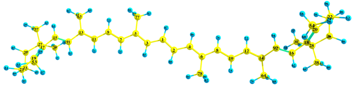
Figure 1: The structure and atom numeration of the C2v symmetry-carotene.

Temperature of the normal vibrational modes, as well as, the phonon modes, is included by performing the Monte Carlo simulation to generate the thermal ensemble of the Davydov $\text{D}_{2}$ wavefunction trajectories. At the zero time, before optical excitation, in each trajectory, the initial coherent state displacements $\tilde{\lambda}_{q}\left(0\right)$, $\lambda_{p}\left(0\right)$ are sampled from the Glauber-Sudarshan distribution ⁵⁵

$$\mathcal{P}\left(\lambda\right)=\mathcal{Z}^{-1}\exp\left(-\left|\lambda\right|^{2}\left(\text{e}^{\frac{\omega}{k_{\text{B}}T}}-1\right)\right),$$ (31)

where $\mathcal{Z}$ is the partition function of a single coherent state $|\lambda\rangle$ with the corresponding frequency $\omega$, $k_{\text{B}}$ is the Boltzmann constant and $T$ is the model temperature. Observables averaged over the thermal ensemble will be denotes as $\left\langle\ldots\right\rangle$. We found $500$ trajectories to be sufficient to obtain converged ensemble for the model of $\beta$-Car as described in the next section.

3 Simulation results

3.1 Normal modes of $\beta$-Car in $S_{0}$ and $S_{2}$ electronic states

We consider a model of $\beta$-Car in thermal equilibrium with a solvent at $300\ \text{K}$. For the photon absorption process, $\beta$-Car is described by the electronic ground state $|S_{0}\rangle\equiv|g\rangle$ and the excited state $|S_{2}\rangle\equiv|e\rangle$. The optically dark excited state $|\text{S}_{1}\rangle$ does not directly participate in electronic absorption process and is excluded.

The electronic Schrödinger equation of the $\beta$-Car molecule was solved using the Density functional theory (DFT) method for the ground electronic state $S_{0}$, and the time-dependent density functional theory (TD-DFT) method for the electronic excited state $S_{2}$, from which atom equilibrium positions $R_{0}^{g}$, $R_{0}^{e}$ are acquired. The GAMESS ⁵⁶ and Gaussian-16 codes ⁵⁷ were used.

The calculation methods were based on the experience from previous calculations of resonance RAMAN spectra of carotenoids, investigation of dependence between the position of the $S_{0}\text{$\rightarrow$}S_{2}$ transition and the frequency of ν1 Raman band ⁵⁸, ⁵⁹. The most RAMAN intense band, ν1, located at around 1500 $\text{cm}^{-1}$, arises from the stretching of the C=C bonds. Previous calculations of the ν1 Raman bands in the ground electronic state $S_{0}$ were performed for another carotenoid, lycopene, using the DFT method with B3LYP/6-31G, B3LYP/TZVP, B3LYP/6-31G(2df,p), BP86/6-31G(d), BPW91/6-31G(d), B3P86/6-31G(d), B3PW91/6-31G(d), and SVWN/6-31G(d) potentials ⁶⁰. It was shown that all methods based on the DFT are able to perform calculation of vibrational frequencies with an overall root-mean-square error of 34−48 $\text{cm}^{-1}$ ⁶¹. Also, it was shown that the dependence of the Raman peak frequency shift, compared between the computed in vacuum and experimental, are linear over the whole spectra ⁵⁸, using the B3LYP/6-311G(d,p) method, a scaling factor 0.9613 has to be used ⁶¹, ⁵⁸. On the other hand, energy of the $\beta$-Car corresponding to the first optically allowed transition in the gas phase was reported to be between 2.85 and 2.93 eV ⁵⁹. This value is 0.62 eV higher than the excitation energy calculated using TD-DFT at the B3LYP/6-311G(d,p) level (2.224 eV) ⁵⁸. Other methods give similar result: Tamm-Dancoff approximation (TDA) blyp/6-31G(d) – 2.15 eV, TD b3lyp/cc-pvdz – 2.19 eV , TD b3lyp/cc-pvtz – 2.21 eV.

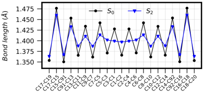
Figure 2: The polyene chain C-C bond lengths in the electronic ground state $S_{0}$ and the excited state $S_{2}$ calculated using the TD-SCF B3LYP/6-311G(d,p) method.

Equilibrium structures of excited states, optimized using the TDA ⁶² and TD-DFT ⁶³, ⁶⁴ with the BLYP functional and DZP basis set, in contrast to B3LYP, yields correct energetic order of the two lowest $\beta$-Car excited states, and it has been shown to reach an accuracy of 0.2 eV for the $S_{1}$ excitation energy in carotenoids ⁶⁵. But later this has been explained by a fortuitous cancellation of errors caused by the neglect of double excitations in the ground and excited states ⁶⁶.

We performed geometry optimization using various methods, with TD-SCF,TDA-SCF basis sets and b3lyp/6-311G(d,p), blyp/6-31G(d), b3lyp/cc-pvdz, b3lyp/cc-pvtz potentials. The Car molecule equilibrium structure and enumeration of atoms is shown in Fig. (1), and the changes of the C-C bond lengths along the Car polyene chain in both electronic states calculated using TD-SCF B3LYP/6-311G(d,p) method is shown in Fig. (2). All tested methods give similar alternation of the C-C bond lengths in $S_{0}$ state, close to that shown in Fig. (2). For the $S_{2}$ state, situation is different – methods using TDA-SCF basis set give alternation similar to the $S_{0}$ state case. The largest alternation of the $S_{2}$ state polyene bond lengths was achieved using the TDA blyp/6-31G(d) method. All TD-SCF calculations provide almost 10 times smaller alternation of C-C bond lengths in the middle of the polyene chain, as compared to the TDA-DTF calculations, again, similar to results shown in Fig. (2).

In order to evaluate influence of the chosen method to the vibrational mode frequencies and their bands, we performed calculation of vibrational spectra using TD-SCF, TDA-SCF methods with different basis sets and potentials (b3lyp/6-311G(d,p), blyp/6-31G(d), b3lyp/cc-pvdz, b3lyp/cc-pvtz). In the $S_{0}$ state, valence vibrational frequencies of the C-C bonds of the polyene chain scale equally and agree to within the range of 20 $\text{cm}^{-1}$. The same vibrational frequencies in the $S_{2}$ state also scale equally, with exception of the TDA blyp/6-31G(d) method, as shown in Fig. (3). All tested methods agree on the C-C bond vibrational frequencies in the $S_{2}$ state within a range of 46 $\text{cm}^{-1}$. Previous ν1 Raman band evaluation and correlation with $S_{0}\text{$\rightarrow$}S_{2}$ excitation in gas phase were performed in vacuum using TD-SCF B3LYP/6-311G(d,p) method and the results shown agreement with the experimental observations ⁵⁸, ⁵⁹. Based on this knowledge, all further presented quantum chemistry calculations were performed in vacuum using B3LYP/6-311G(d,p) method as in Ref. ⁵⁹ and scaling factor was not applied.

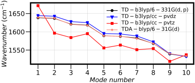
Figure 3: Polyene backbone C-C valence vibrational mode frequencies in the excited state $S_{2}$ calculated using various quantum chemistry methods.

The changes in polyene chain geometry during $S_{0}\text{$\rightarrow$}S_{2}$ electronic excitation causes changes in molecular electronic structure, normal mode frequencies and vibrational mode coordinates. The C–H valence bond vibrations in all $\beta$-Car parts are in the region of 2970–3170 $\text{cm}^{-1}$ for the ground state, and in the region of 2960-3168 $\text{cm}^{-1}$ for the excited state. The lower frequency region is characterized by the change of C=C bond lengths in polyene chain. Here, the $S_{0}$ normal mode frequencies lay in the region of 1558-1674 $\text{cm}^{-1}$ and the corresponding region for $S_{2}$ state is 1533-1636 $\text{cm}^{-1}$. Transition $S_{0}\rightarrow S_{2}$ mainly induces differences in the polyene chain bond lengths between carbon atoms in both electronic states. As a consequence, vibrational frequencies in the $S_{2}$ state become lower by 40-50 $\text{cm}^{-1}$.

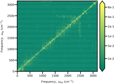
Figure 4: Expansion coefficient absolute value $\left|a_{kj}^{(eg)}\right|$ of the $\beta$-Car normal modes. The $k$th mode in the $S_{2}$ state in expanded in terms of the mode $j$th in the state $S_{0}$ calculated using the TD-SCF B3LYP/6-311G(d,p) method.

Expressing normal mode coordinates in the electronic state $S_{2}$ by normal coordinates of the ground electronic state $S_{0}$, according to the Eq. (12), allows to investigate normal mode mixing upon $S_{0}\rightarrow S_{2}$ electronic transition. In Fig. (4) we plot expansion coefficient absolute value $\left|a_{kj}^{(eg)}\right|$, i.e., the $k$th mode in the $S_{2}$ state in expanded in terms of the mode $j$th in the state $S_{0}$. Largest expansion coefficients lay close the main diagonal, implying that the majority of normal modes are non-negligibly mixed with similar frequency modes. However, certain modes show mixing with modes that has a vastly different frequencies, e.g., modes in a frequency region of $\approx 2500\ \text{cm}^{-1}$ are highly mixed with modes in a frequency range of $1500-2500\ \text{cm}^{-1}$. Strong mixing can also be clearly seen between modes in frequency regions of $0-250\ \text{cm}^{-1}$, $400-750\ \text{cm}^{-1}$, $1000-1500\ \text{cm}^{-1}$. Such a broad frequency mixing range signifies wide range of available vibrational relaxation pathways. At a first glance, expansion coefficients along the $\omega_{ei}=\omega_{gi}$ diagonal may look symmetric, however, they are not, even when absolute values are considered $\left|a_{kj}^{(eg)}\right|\neq\left|a_{jk}^{(eg)}\right|$. This demonstrates that there is no one-to-one correspondence between the $\beta$-Car normal modes in electronic $S_{0}$ and $S_{2}$ states.

Additionaly, we found that during transitions between $S_{0}$ and $S_{2}$ electronic states, transition dipole moment remain comparable. For transition $S_{0}\text{$\rightarrow$}S_{2}$, the transition moment components are $\mu_{02}=\left(8.35,0.71,0.0\right)$ in a.u. $\left(21.28\ \text{Debye}\right)$, while for the $S_{2}\text{$\rightarrow$}S_{0}$, it is equal to $\mu_{20}=\left(9.45,0.57,0.0\right)$ in a.u. $\left(24.06\ \text{Debye}\right)$. Difference between the two transitions are minimal, thus non-Condon effects can be reasonably excluded from calculations. Transition dipole moment is oriented with z component being perpendicular to the plane of polyene chain, while x component is directed along the polyene chain.

3.2 Absorption spectrum of the $\beta$-carotene model

The quantum chemistry results of the $\beta$-Car is now used to compute the absorption spectrum given by the Eq. (7). The Fourier transformation is performed on the linear response function averaged over the thermal ensemble, $\left\langle F\left(t\right)\right\rangle$, single trajectory of the ensemble linear response is defined in the Eq. (8), and equal to

$$F\left(t\right)=\left|\bm{\mu}_{eg}^{(\text{el})}\right|^{2}\text{e}^{\frac{\text{i}}{2}\sum_{k}\omega_{gk}t}\alpha_{g}^{\star}\left(0\right)\alpha_{e}\left(t\right)\\ \times\text{$\exp$$\sum_{k}$$\left(\text{e}^{\text{i}\omega_{gk}t}\tilde{\lambda}_{k}^{\star}\left(0\right)\tilde{\lambda}_{k}\left(t\right)-\frac{1}{2}\left(\left|\tilde{\lambda}_{k}\left(0\right)\right|^{2}+\left|\tilde{\lambda}_{k}\left(t\right)\right|^{2}\right)\right)$}\\ \times\text{$\exp$$\sum_{p}$$\left(\text{e}^{\text{i}w_{p}t}\lambda_{p}^{\star}\left(0\right)\lambda_{p}\left(t\right)-\frac{1}{2}\left(\left|\lambda_{p}\left(0\right)\right|^{2}+\left|\lambda_{p}\left(t\right)\right|^{2}\right)\right)$}.$$ (32)

It is expressed in terms of the dynamical parameters $\alpha_{n}$$\left(t\right)$, $\tilde{\lambda}_{k}\left(t\right)$, $\lambda_{p}\left(t\right)$, therefore it is enough to propagate the excited state dynamics.

For the solvent, the phonon bath modes are defined by uniformly discretizing the spectral density function $C_{e}^{"}\left(\omega\right)$ in frequency domain in the range $\left[w_{\text{min}}=0.1,\ w_{\text{max}}=1250\right]\ \text{cm}^{-1}$ with discretization step size $\Delta_{w}=10\ \text{cm}^{-1}$. Then the frequency of $p$th bath mode is given by $w_{p}=w_{\text{min}}+\left(p-1\right)\Delta_{w}$. Form of the spectral density function was chosen to be the Overdamped Brownian oscillator function $C_{e}^{"}\left(w\right)=2\Lambda_{e}^{\mathrm{ph}}\omega\gamma/(\omega^{2}+\gamma^{2})$. Damping parameter $\gamma=200\ \text{cm}^{-1}$ $\left(167\ \text{fs}\right)$ has been chosen based on the previous modeling of $\beta$-Car ⁶⁷ spectra. Amplitude of the spectral density function is set by normalizing $f_{ep}$ values according to the reorganization energy definition by the Eq. (24). The bath reorganization energy of $\Lambda_{e}^{\text{ph}}=100\ \text{cm}^{-1}$ have been chosen to qualitatively match the line widths of the experimental data.

The simulated absorption spectrum of $\beta$-Car model with 282 normal modes at different temperatures is shown in Fig. (5) along the experimental $\beta$-Car spectrum in diethylamine solvent at room temperature ²⁷. Absorption spectra have been normalized to their maximum value, as well as, aligned on the 0-0 transition band for easier comparison. We find the 282-mode model spectrum to qualitatively reproduce position and amplitudes of the first two absorption peaks, however, it greatly overestimates the amplitude of vibrational peak progression at $300$ K temperature. Also, absorption of the high frequency modes display non-trivial dependence on the temperature. For majority of modes the average thermal energy is much smaller than the energy gap between the vibrational mode energy levels, $k_{\text{B}}T\ll\omega$, thus, for non-mixed modes, dependence of absorption spectrum on temperature would be negligible. However, in Fig. (5) we observe strong dependence of absorption on temperature due to the mode mixing, i.e., thermally excited low frequency vibrational modes contribute to the excitation of the high frequency modes, which results in a wide high frequency absorption shoulder.

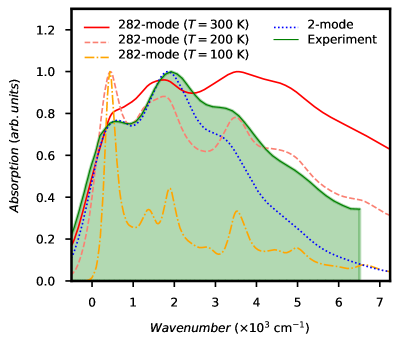
Figure 5: Absorption spectra of $\beta$-Car model, based on B3LYP/6-311G(d,p) method, at different temperatures along the experimental $\beta$-Car spectrum in diethylamine solvent at room temperature (shown as contoured green). The widely used 2-mode model at 300 K temperature is also shown for comparison, model parameters are taken from Ref. ²³. All spectra are normalized to their maximum value and aligned on their 0-0 transition band.

For comparison, we also computed absorption spectrum of a widely used empirical 2-mode $\beta$-Car model at $300$ K temperature, which includes only the C=C and C-C stretching vibrational modes with no mixing between them. Typical model frequencies $\omega_{\text{e,C=C}}=1522\ \text{cm}^{-1}$, $\omega_{e,\text{C-C}}=1157\ \text{cm}^{-1}$ and displacements $d_{\text{C=C}}^{\left(eg\right)}=1.3$, $d_{\text{C-C}}^{\left(eg\right)}=0.9$ are taken from Ref. ²³. To have correct line widths, bath reorganization energy is now set to a much larger $\Lambda_{e}^{\text{ph}}=800\ \text{cm}^{-1}$, this is to account for the lack of the rest $\beta$-Car modes. As shown in Fig. (5), the 2-mode model fits first two peaks well, but underestimates amplitude of the higher frequency progression.

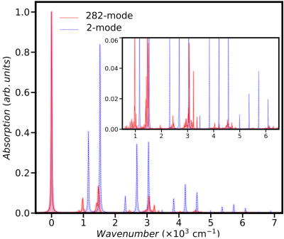
Figure 6: Stick absorption spectrum of the 282-mode model, computed using the B3LYP/6-311G(d,p) method, and the empirical 2-mode model. Purely electronic transition energy is set to $0\ \text{cm}^{-1}$ for both spectra. For visibility, each spectra have been convoluted with the $\tau=1\ \text{ps}$ variance Gaussian function. Inset more closely shows low amplitude sticks, and these has been convoluted with $\tau=5\ \text{ps}$ variance Gaussian function.

To further compare the 282-mode and the 2-mode models, we look at their stick absorption spectrum in Fig. (6). The purely electronic transition energy is set to $0\ \text{cm}^{-1}$ for both spectra. For visibility, spectra have been convoluted with the $\tau=1\ \text{ps}$ variance Gaussian function, $\tau=5\ \text{ps}$ is used for spectra in the inset. The 2-mode model stick spectrum has a straightforward peak progression, i.e., spectrum is a sum of each of the two mode peak progressions. The 282-mode model spectrum has a more complex structure. Even though each of the 282 modes have a small absorption peak, the combined spectrum produces frequency regions with non-negligible absorption intensity. These regions show clear overlap with the absorption peaks of the 2-mode model. The 2-mode spectrum has peaks at $1522\ \text{cm}^{-1}$ and $1157\ \text{cm}^{-1}$ frequencies, produced by the C=C and C-C stretching vibrational modes. The 282-mode spectrum has similar frequency regions, only this time, they are due to the absorption of a large number of mixed normal modes. These modes are responsible for the first two peaks seen in Fig. (5) spectra.

Looking further on in Fig. (6), the 282-mode model has absorption in the $3000\ \text{cm}^{-1}$, $4500\ \text{cm}^{-1}$, $6000\ \text{cm}^{-1}$ frequency regions. These account for the high frequency absorption tail seen in experiments. Due to the C=C and C-C mode progression, the 2-mode model has a peak at these frequencies as well, however, even though visually they look more intese than the 282-mode model peaks, Fig. (5) simulations show it being the opposite. Again, the strong absorption is produced by the summation of a large number of weak intensity absorption peaks. Two harmonic modes simply can not accurately describe absorption over a such a wide range of frequencies, therefore, the high frequency absorption of the 2-mode model is lacking.

4 Discussion

Vibrational modes of carotenoids have been extensively studied by Raman spectroscopy ⁶⁸, ⁶⁹. The frequency of the most Raman active V1 vibration in the $S_{0}$ state is 1642.3 $\text{cm}^{-1}$, which changes to a week Raman vibration of frequency 1584.08 $\text{cm}^{-1}$ in the $S_{2}$ state. The C-C valence bond frequencies in $S_{0}$ state lay in the region of 1018-1353 $\text{cm}^{-1}$, while it is in region of 1156-1370 $\text{cm}^{-1}$ for the $S_{2}$ state. These frequencies are strongly mixed with the polyene chain C-H bond in-plane vibrations, and the C-C valence vibrations of peripheral rings. The strongest V2 Raman active vibration in this region, for the $S_{0}$ state, is 1187.22 $\text{cm}^{-1}$, while the mode with the most similar vibrational form in the $S_{2}$ state has a frequency of 1219 $\text{cm}^{-1}$. Vibrations of lower frequencies are associated with the C-H vibrations outside of the polyene chain, deformations of the peripheral rings, changes of the polyene chain valence angles, dihedral angles and the deformations of the whole molecule by twisting and waving. Frequencies of these vibrations change by no more than 10 $\text{cm}^{-1}$ after the $S_{0}\rightarrow S_{2}$ transition. Difference in the vibrational forms are not as strong for these modes, as were in the case of the polyene chain C-C and C=C valence bond vibrations.

Recently Balevičius Jr. and co-workers ²⁰ have presented an in-depth excitation energy relaxation model in carotenoids by considering four relaxation processes. Simply put, the event of photoexcitation instantaneously promotes the carotenoid molecules to a non-equilibrium state and launches the internal vibrational redistribution (IVR) cascade within the high-frequency optically active modes resulting into transient thermally "hot" state. Generally, it is assumed that the thermally hot carotenoid subsequently transfers vibrational energy to the solvent molecules, i.e., vibrational cooling (VC) takes place. Authors demonstrated how modeling the IVR and VC concurrently, and not subsequently, naturally explains the presence of the highly discussed transient absorption $S^{*}$ signal ⁷⁰ in terms of the vibrationally hot ground state $S_{0}$. The 2-mode model was used, i.e., only the C-C and C=C intramolecular modes were coupled to the thermal bath - their coupling strength remains speculative. Both the IVC and VC relaxation were modeled implicitly by prescribing process timescales. We have shown that the 2-mode (not mixed) model is not sufficient in describing the photon absorption spectrum. In fact, upon photoexcitation many vibrational modes become excited. No two distinctive modes could be isolated in the relevant frequency region. We observe grouping of vibrational modes in the $1000\ \text{cm}^{-1}$ and $1500\ \text{cm}^{-1}$ frequency regions, as shown in Fig. 6. The 2-mode model yields progression of peaks with few strong features at $2700\ \text{cm}^{-1}$ and $4000-6000\ \text{cm}^{-1}$ frequencies. Meanwhile, the 282-mode model has a large number of weak absorption features at these frequencies, however, it is the cumulative effect that combines them into the observed "progression". This entropic factor actually simplifies the overall electronic excitation relaxation picture since each mode is weakly coupled to the electronic transition, therefore, the weak coupling regime could be used in theoretical models of relaxation dynamics. Consequently, the two- or multiple-quanta vibrational excitations become improbable. Hence, only the entropic factor as a cumulative effect of all modes would have decisive impact on both the IVR and VC processes timescales.

In Nature carotenoids participate in energy conversion process together with other types of pigments. Carotenoids play an important role in light-harvesting complexes by transfers their excitation to chlorophylls on a femtosecond timescale. It is especially evident in the peridinin–chlorophyll a protein (PCP), in which the dominant energy transfer occurs from the peridinin $S_{2}$ to chlorophyll $Q_{y}$ state via an ultrafast coherent mechanism. The coherent superposition of the two states functions in a way as to drive the population to the final acceptor state ⁷¹, providing an important piece of evidence in the quest of connecting coherent phenomena and biological functions ⁷². This process is highly sensitive to structural perturbations of the peridinin polyene backbone, which has a profound effect on the overall lifetime of the complex ⁷³. We have found that $\beta$-Car as well undergoes polyene backbone changes, mainly, in its C-C bond lengths.

As well, it has been suggested that the ultrafast population transfer from the carotenoid state $S_{2}$ to the bacteriochlorophyll (BChl) state $Q_{x}$ occurs due to the vibronic coupling of the carotenoid electron-vibrational degrees of freedom to the BChl ⁷⁴. Energy flow pathway opened up by the resonance of the energy gap between the carotenoid vibrational levels, and the BChl $|g\rangle_{\text{BChl}}\rightarrow|Q_{x}\rangle$ transition is the primary reason for its ultrafast nature. We, hence, suggest, that by going beyond the 2-mode model and taking into account more carotenoid vibrational modes, in turn, more vibrational levels, the probability of resonance between the carotenoid and BChl would greatly increased, changing the overall population transfer rate.

In conclusion, we have presented a $\beta$-Car model with fully explicit treatment of all its 282 vibrational normal modes, which were computed using the quantum chemical methods. Additionally, we described how to treat the $\beta$-Car excited states dynamics when in contact with solvent at finite temperature. We found $\beta$-Car to change bond lengths between the polyene chain atoms during the $S_{0}\rightarrow S_{2}$ electronic transition, as well as, that the there is no one-to-one correspondence between the ground and the excited state vibrational modes, i.e., modes on different electronic states are highly mixed and should not be treated as being the same. Model absorption spectrum qualitatively match the experimental data, it better describe the high frequency progression of the carotenoid spectrum than the typical 2-mode carotenoid model. Derivation of the Davydov $D_{2}$ ansatz equations of motion for the $\beta$-carotene model using Dirac-Frenkel variational method. We thank the Research Council of Lithuania for financial support (grant No: S-MIP-20-47). Computations were performed on resources at the High Performance Computing Center, “HPC Sauletekis” in Vilnius University Faculty of Physics.

References

- Tian 2015 Tian, L. Recent advances in understanding carotenoid-derived signaling molecules in regulating plant growth and development. Front. Plant Sci. 2015, 6, 790
- Weaver et al. 2018 Weaver, R. J.; Santos, E. S.; Tucker, A. M.; Wilson, A. E.; Hill, G. E. Carotenoid metabolism strengthens the link between feather coloration and individual quality. Nat. Commun. 2018, 9, 73
- Murchie and Harbinson 2014 Murchie, E. H.; Harbinson, J. Non-Photochemical Fluorescence Quenching Across Scales: From Chloroplasts to Plants to Communities; Springer, Dordrecht, 2014; pp 553–582
- Ruban 2016 Ruban, A. V. Nonphotochemical chlorophyll fluorescence quenching: Mechanism and effectiveness in protecting plants from photodamage. Plant Physiol. 2016, 170, 1903–1916
- Ruban et al. 2007 Ruban, A. V.; Berera, R.; Ilioaia, C.; Van Stokkum, I. H.; Kennis, J. T.; Pascal, A. A.; Van Amerongen, H.; Robert, B.; Horton, P.; Van Grondelle, R. Identification of a mechanism of photoprotective energy dissipation in higher plants. Nature 2007, 450, 575–578
- Holt et al. 2005 Holt, N. E.; Zigmantas, D.; Valkunas, L.; Li, X. P.; Niyogi, K. K.; Fleming, G. R. Carotenoid cation formation and the regulation of photosynthetic light harvesting. Science 2005, 307, 433–436
- Llansola-Portoles et al. 2017 Llansola-Portoles, M. J.; Sobotka, R.; Kish, E.; Shukla, M. K.; Pascal, A. A.; Polívka, T.; Robert, B. Twisting a -carotene, an adaptive trick from nature for dissipating energy during photoprotection. J. Biol. Chem. 2017, 292, 1396–1403
- Bode et al. 2009 Bode, S.; Quentmeier, C. C.; Liao, P. N.; Hafi, N.; Barros, T.; Wilk, L.; Bittner, F.; Walla, P. J. On the regulation of photosynthesis by excitonic interactions between carotenoids and chlorophylls. Proc. Natl. Acad. Sci. U. S. A. 2009, 106, 12311–12316
- Cupellini et al. 2020 Cupellini, L.; Calvani, D.; Jacquemin, D.; Mennucci, B. Charge transfer from the carotenoid can quench chlorophyll excitation in antenna complexes of plants. Nat. Commun. 2020, 11, 1–8
- Polívka and Sundström 2004 Polívka, T.; Sundström, V. Ultrafast dynamics of carotenoid excited states-from solution to natural and artificial systems. Chem. Rev. 2004, 104, 2021–2071
- Llansola-Portoles et al. 2017 Llansola-Portoles, M. J.; Pascal, A. A.; Robert, B. Electronic and vibrational properties of carotenoids: from in vitro to in vivo. J. R. Soc. Interface 2017, 14, 20170504
- Bautista et al. 1999 Bautista, J. A.; Connors, R. E.; Raju, B. B.; Hiller, R. G.; Sharples, F. P.; Gosztola, D.; Wasielewski, M. R.; Frank, H. A. Excited State Properties of Peridinin: Observation of a Solvent Dependence of the Lowest Excited Singlet State Lifetime and Spectral Behavior Unique among Carotenoids. J. Phys. Chem. B 1999, 103, 8751–8758
- Frank et al. 2000 Frank, H. A.; Bautista, J. A.; Josue, J.; Pendon, Z.; Hiller, R. G.; Sharples, F. P.; Gosztola, D.; Wasielewski, M. R. Effect of the Solvent Environment on the Spectroscopic Properties and Dynamics of the Lowest Excited States of Carotenoids. J. Phys. Chem. B 2000, 104, 4569–4577
- Tamm 1991 Tamm, I. Relativistic Interaction of Elementary Particles. Sel. Pap. 1991, 9, 157–174
- Dancoff 1950 Dancoff, S. M. Non-adiabatic meson theory of nuclear forces. Phys. Rev. 1950, 78, 382–385
- Andreussi et al. 2015 Andreussi, O.; Knecht, S.; Marian, C. M.; Kongsted, J.; Mennucci, B. Carotenoids and light-harvesting: From DFT/MRCI to the Tamm-Dancoff approximation. J. Chem. Theory Comput. 2015, 11, 655–666
- Vaswani et al. 2003 Vaswani, H. M.; Hsu, C. P.; Head-Gordon, M.; Fleming, G. R. Quantum chemical evidence for an intramolecular charge-transfer state in the carotenoid peridinin of peridinin-chlorophyll-protein. J. Phys. Chem. B 2003, 107, 7940–7946
- Hashimoto et al. 2018 Hashimoto, H.; Uragami, C.; Yukihira, N.; Gardiner, A. T.; Cogdell, R. J. Understanding/unravelling carotenoid excited singlet states. J. R. Soc. Interface 2018, 15, 20180026
- Premvardhan et al. 2005 Premvardhan, L.; Papagiannakis, E.; Hiller, R. G.; Van Grondelle, R. The charge-transfer character of the S0 S2 transition in the carotenoid peridinin is revealed by stark spectroscopy. J. Phys. Chem. B 2005, 109, 15589–15597
- Balevičius et al. 2019 Balevičius, V.; Wei, T.; Di Tommaso, D.; Abramavicius, D.; Hauer, J.; Polívka, T.; Duffy, C. D. The full dynamics of energy relaxation in large organic molecules: From photo-excitation to solvent heating. Chem. Sci. 2019, 10, 4792–4804
- Mendes-Pinto et al. 2013 Mendes-Pinto, M. M.; Sansiaume, E.; Hashimoto, H.; Pascal, A. A.; Gall, A.; Robert, B. Electronic absorption and ground state structure of carotenoid molecules. J. Phys. Chem. B 2013, 117, 11015–11021
- Wei et al. 2019 Wei, T.; Balevičius, V.; Polívka, T.; Ruban, A. V.; Duffy, C. D. How carotenoid distortions may determine optical properties: Lessons from the orange carotenoid protein. Phys. Chem. Chem. Phys. 2019, 21, 23187–23197
- Polívka et al. 2001 Polívka, T.; Zigmantas, D.; Frank, H. A.; Bautista, J. A.; Herek, J. L.; Koyama, Y.; Fujii, R.; Sundström, V. Near-infrared time-resolved study of the S1 state dynamics of the carotenoid spheroidene. J. Phys. Chem. B 2001, 105, 1072–1080
- Christensson et al. 2009 Christensson, N.; Milota, F.; Nemeth, A.; Sperling, J.; Kauffmann, H. F.; Pullerits, T.; Hauer, J. Two-dimensional electronic spectroscopy of -carotene. J. Phys. Chem. B 2009, 113, 16409–16419
- Balevičius et al. 2016 Balevičius, V.; Abramavicius, D.; Polívka, T.; Galestian Pour, A.; Hauer, J. A Unified Picture of S* in Carotenoids. J. Phys. Chem. Lett. 2016, 7, 3347–3352
- Fox et al. 2017 Fox, K. F.; Balevičius, V.; Chmeliov, J.; Valkunas, L.; Ruban, A. V.; Duffy, C. D. The carotenoid pathway: What is important for excitation quenching in plant antenna complexes? Phys. Chem. Chem. Phys. 2017, 19, 22957–22968
- Gong et al. 2018 Gong, N.; Fu, H.; Wang, S.; Cao, X.; Li, Z.; Sun, C.; Men, Z. All-trans--carotene absorption shift and electron-phonon coupling modulated by solvent polarizability. J. Mol. Liq. 2018, 251, 417–422
- Valkunas et al. 2013 Valkunas, L.; Abramavicius, D.; Mancal, T. Molecular Excitation Dynamics and Relaxation; John Wiley & Sons, Ltd, 2013
- May and Kühn 2011 May, V.; Kühn, O. Charg. Energy Transf. Dyn. Mol. Syst. Third Ed.; Wiley-VCH Verlag GmbH & Co. KGaA: Weinheim, Germany, 2011
- Letokhov 1998 Letokhov, V. Uspekhi Fiz. Nauk; Oxford University Press, 1998; Vol. 168; p 591
- Duschinsky 1937 Duschinsky, F. On the Interpretation of Eletronic Spectra of Polyatomic Molecules. Acta Physicochim. U.R.S.S. 1937, 7, 551–566
- Sando et al. 2001 Sando, G. M.; Spears, K. G.; Hupp, J. T.; Ruhoff, P. T. Large electron transfer rate effects from the Duschinsky mixing of vibrations. J. Phys. Chem. A 2001, 105, 5317–5325
- Meier and Rauhut 2015 Meier, P.; Rauhut, G. Comparison of methods for calculating Franck-Condon factors beyond the harmonic approximation: How important are Duschinsky rotations? Mol. Phys. 2015, 113, 3859–3873
- Yan and Mukamel 1986 Yan, Y. J.; Mukamel, S. Eigenstate-free, Green function, calculation of molecular absorption and fluorescence line shapes. J. Chem. Phys. 1986, 85, 5908–5923
- Borrelli and Peluso 2003 Borrelli, R.; Peluso, A. Dynamics of radiationless transitions in large molecular systems: A Franck-Condon-based method accounting for displacements and rotations of all the normal coordinates. J. Chem. Phys. 2003, 119, 8437–8448
- Ianconescu and Pollak 2004 Ianconescu, R.; Pollak, E. Photoinduced cooling of polyatomic molecules in an electronically excited state in the presence of dushinskii rotations. J. Phys. Chem. A 2004, 108, 7778–7784
- Borrelli et al. 2013 Borrelli, R.; Capobianco, A.; Peluso, A. Franck-Condon factors-Computational approaches and recent developments. Can. J. Chem. 2013, 91, 495–504
- Niu et al. 2010 Niu, Y.; Peng, Q.; Deng, C.; Gao, X.; Shuai, Z. Theory of excited state decays and optical spectra: Application to polyatomic molecules. J. Phys. Chem. A 2010, 114, 7817–7831
- Borrelli et al. 2012 Borrelli, R.; Capobianco, A.; Peluso, A. Generating function approach to the calculation of spectral band shapes of free-base chlorin including Duschinsky and Herzberg-Teller effects. J. Phys. Chem. A 2012, 116, 9934–9940
- Baiardi et al. 2013 Baiardi, A.; Bloino, J.; Barone, V. General time dependent approach to vibronic spectroscopy including franck-condon, herzberg-teller, and duschinsky effects. J. Chem. Theory Comput. 2013, 9, 4097–4115
- Toutounji 2020 Toutounji, M. Spectroscopy of Vibronically Coupled and Duschinskcally Rotated Polyatomic Molecules. J. Chem. Theory Comput. 2020, 16, 1690–1698
- Davydov 1979 Davydov, A. S. Solitons in molecular systems. Phys. Scr. 1979, 20, 387–394
- Scott 1991 Scott, A. C. Davydov’s soliton revisited. Phys. D Nonlinear Phenom. 1991, 51, 333–342
- Choi 2004 Choi, J. R. Coherent states of general time-dependent harmonic oscillator. Pramana - J. Phys. 2004, 62, 13–29
- Sun et al. 2010 Sun, J.; Luo, B.; Zhao, Y. Dynamics of a one-dimensional Holstein polaron with the Davydov ansätze. Phys. Rev. B - Condens. Matter Mater. Phys. 2010, 82, 014305
- Chorošajev et al. 2016 Chorošajev, V.; Rancova, O.; Abramavicius, D. Polaronic effects at finite temperatures in the B850 ring of the LH2 complex. Phys. Chem. Chem. Phys. 2016, 18, 7966–7977
- Wang et al. 2016 Wang, L.; Chen, L.; Zhou, N.; Zhao, Y. Variational dynamics of the sub-Ohmic spin-boson model on the basis of multiple Davydov D1 states. J. Chem. Phys. 2016, 144, 024101
- Jakučionis et al. 2018 Jakučionis, M.; Chorošajev, V.; Abramavičius, D. Vibrational damping effects on electronic energy relaxation in molecular aggregates. Chem. Phys. 2018, 515, 193–202
- Jakučionis et al. 2020 Jakučionis, M.; Mancal, T.; Abramavičius, D. Modeling irreversible molecular internal conversion using the time-dependent variational approach with sD2 ansatz. Phys. Chem. Chem. Phys. 2020, 22, 8952–8962
- Sun et al. 2015 Sun, K. W.; Gelin, M. F.; Chernyak, V. Y.; Zhao, Y. Davydov Ansatz as an efficient tool for the simulation of nonlinear optical response of molecular aggregates. J. Chem. Phys. 2015, 142, 212448
- Zhou et al. 2016 Zhou, N.; Chen, L.; Huang, Z.; Sun, K.; Tanimura, Y.; Zhao, Y. Fast, Accurate Simulation of Polaron Dynamics and Multidimensional Spectroscopy by Multiple Davydov Trial States. J. Phys. Chem. A 2016, 120, 1562–1576
- Chorošajev et al. 2017 Chorošajev, V.; Marčiulionis, T.; Abramavicius, D. Temporal dynamics of excitonic states with nonlinear electron-vibrational coupling. J. Chem. Phys. 2017, 147, 74114
- Somoza et al. 2017 Somoza, A. D.; Sun, K. W.; Molina, R. A.; Zhao, Y. Dynamics of coherence, localization and excitation transfer in disordered nanorings. Phys. Chem. Chem. Phys. 2017, 19, 25996–26013
- Chen et al. 2019 Chen, L.; Gelin, M. F.; Domcke, W. Multimode quantum dynamics with multiple Davydov D2 trial states: Application to a 24-dimensional conical intersection model. J. Chem. Phys. 2019, 150, 24101
- Glauber 1963 Glauber, R. J. Coherent and incoherent states of the radiation field. Phys. Rev. 1963, 131, 2766–2788
- Schmidt et al. 1993 Schmidt, M. W.; Baldridge, K. K.; Boatz, J. A.; Elbert, S. T.; Gordon, M. S.; Jensen, J. H.; Koseki, S.; Matsunaga, N.; Nguyen, K. A.; Su, S. et al. General atomic and molecular electronic structure system. J. Comput. Chem. 1993, 14, 1347–1363
- Frisch et al. 2016 Frisch, M. J.; Trucks, G. W.; Schlegel, H. B.; Scuseria, G. E.; Robb, M. A.; Cheeseman, J. R.; Scalmani, G.; Barone, V.; Petersson, G. A.; Nakatsuji, H. et al. Gaussian 16 Revision C.01. 2016; Gaussian Inc. Wallingford CT
- Macernis et al. 2014 Macernis, M.; Sulskus, J.; Malickaja, S.; Robert, B.; Valkunas, L. Resonance raman spectra and electronic transitions in carotenoids: A density functional theory study. J. Phys. Chem. A 2014, 118, 1817–1825
- Macernis et al. 2015 Macernis, M.; Galzerano, D.; Sulskus, J.; Kish, E.; Kim, Y. H.; Koo, S.; Valkunas, L.; Robert, B. Resonance Raman spectra of carotenoid molecules: Influence of methyl substitutions. J. Phys. Chem. A 2015, 119, 56–66
- Liu et al. 2010 Liu, W. L.; Wang, D. M.; Zheng, Z. R.; Li, A. H.; Su, W. H. Solvent effects on the S0 S2 absorption spectra of -carotene. Chinese Phys. B 2010, 19, 013102–6
- Wong 1996 Wong, M. W. Vibrational frequency prediction using density functional theory. Chem. Phys. Lett. 1996, 256, 391–399
- Hirata and Head-Gordon 1999 Hirata, S.; Head-Gordon, M. Time-dependent density functional theory within the Tamm-Dancoff approximation. Chem. Phys. Lett. 1999, 314, 291–299
- Casida 1995 Casida, M. E. Time-Dependent Density Functional Response Theory for Molecules; 1995; pp 155–192
- Dreuw and Head-Gordon 2005 Dreuw, A.; Head-Gordon, M. Single-reference ab initio methods for the calculation of excited states of large molecules. Chem. Rev. 2005, 105, 4009–4037
- Dreuw 2006 Dreuw, A. Influence of geometry relaxation on the energies of the S1 and S2 states of violaxanthin, zeaxanthin, and lutein. J. Phys. Chem. A 2006, 110, 4592–4599
- Starcke et al. 2006 Starcke, J. H.; Wormit, M.; Schirmer, J.; Dreuw, A. How much double excitation character do the lowest excited states of linear polyenes have? Chem. Phys. 2006, 329, 39–49
- Balevičius et al. 2015 Balevičius, V.; Pour, A. G.; Savolainen, J.; Lincoln, C. N.; Lukeš, V.; Riedle, E.; Valkunas, L.; Abramavicius, D.; Hauer, J. Vibronic energy relaxation approach highlighting deactivation pathways in carotenoids. Phys. Chem. Chem. Phys. 2015, 17, 19491–19499
- de Oliveira et al. 2010 de Oliveira, V. E.; Castro, H. V.; Edwards, H. G.; de Oliveiraa, L. F. C. Carotenes and carotenoids in natural biological samples: A Raman spectroscopic analysis. J. Raman Spectrosc. 2010, 41, 642–650
- Tschirner et al. 2009 Tschirner, N.; Schenderlein, M.; Brose, K.; Schlodder, E.; Mroginski, M. A.; Thomsen, C.; Hildebrandt, P. Resonance Raman spectra of -carotene in solution and in photosystems revisited: an experimental and theoretical study. Phys. Chem. Chem. Phys. 2009, 11, 11471–11478
- Polívka and Sundström 2009 Polívka, T.; Sundström, V. Dark excited states of carotenoids: Consensus and controversy. Chem. Phys. Lett. 2009, 477, 1–11
- Roscioli et al. 2017 Roscioli, J. D.; Ghosh, S.; LaFountain, A. M.; Frank, H. A.; Beck, W. F. Quantum Coherent Excitation Energy Transfer by Carotenoids in Photosynthetic Light Harvesting. J. Phys. Chem. Lett. 2017, 8, 5141–5147
- Meneghin et al. 2018 Meneghin, E.; Volpato, A.; Cupellini, L.; Bolzonello, L.; Jurinovich, S.; Mascoli, V.; Carbonera, D.; Mennucci, B.; Collini, E. Coherence in carotenoid-to-chlorophyll energy transfer. Nat. Commun. 2018, 9, 3160
- Ghosh et al. 2017 Ghosh, S.; Bishop, M. M.; Roscioli, J. D.; LaFountain, A. M.; Frank, H. A.; Beck, W. F. Excitation Energy Transfer by Coherent and Incoherent Mechanisms in the Peridinin-Chlorophyll a Protein. J. Phys. Chem. Lett. 2017, 8, 463–469
- Perlík et al. 2015 Perlík, V.; Seibt, J.; Cranston, L. J.; Cogdell, R. J.; Lincoln, C. N.; Savolainen, J.; Šanda, F.; Mančal, T.; Hauer, J. Vibronic coupling explains the ultrafast carotenoid-to-bacteriochlorophyll energy transfer in natural and artificial light harvesters. J. Chem. Phys. 2015, 142, 212434