Transcendental Idealism of Planner:
Evaluating Perception from Planning Perspective for Autonomous Driving

Abstract

Evaluating the performance of perception modules in autonomous driving is one of the most critical tasks in developing the complex intelligent system. While module-level unit test metrics adopted from traditional computer vision tasks are feasible to some extent, it remains far less explored to measure the impact of perceptual noise on the driving quality of autonomous vehicles in a consistent and holistic manner. In this work, we propose a principled framework that provides a coherent and systematic understanding of the impact an error in the perception module imposes on an autonomous agent’s planning that actually controls the vehicle. Specifically, the planning process is formulated as expected utility maximisation, where all input signals from upstream modules jointly provide a world state description, and the planner strives for the optimal action by maximising the expected utility determined by both world states and actions. We show that, under practical conditions, the objective function can be represented as an inner product between the world state description and the utility function in a Hilbert space. This geometric interpretation enables a novel way to analyse the impact of noise in world state estimation on planning and leads to a universal metric for evaluating perception. The whole framework resembles the idea of transcendental idealism in the classical philosophical literature, which gives the name to our approach.

1 Introduction

Autonomous driving has recently emerged as a rapidly advancing realm in both academia and industry, attracting a surge of interest from scientific and engineering communities. As a complex system, an autonomous vehicle (AV) comprises numerous hardware components and interactive onboard modules. One such core component is the onboard perception module (Feng et al., 2022), which serves as the major source of real-time characterisation of the dynamic and stochastic environment an AV navigates through.

To evaluate and improve the perception module, conventional perception tasks (such as detection and tracking) have been well-defined and established with corresponding performance measurements in computer vision for benchmarking (Lin et al., 2014; Caesar et al., 2020). Despite their great success in advancing perceptual information processing modules, almost all such metrics exclusively focus on the perception-centric performance in a deployment-agnostic fashion, ignoring the actual impact of the result to the entire AV system. Indeed, not all perception errors render the same consequence on AV planning: missing an obstacle in front of an AV moving forward is obviously far more serious than one behind. This problem is further compounded by the heterogeneity of perceptual errors that share few semantics in common (‘How does an error of 5m/s in velocity compare to that of a size 25% larger?’), where manual engineering based on intuition is widely adopted (Caesar et al., 2020; Deng et al., 2021). Although these issues are typically addressed through integration road tests in the real world, the process is extremely costly and time-consuming, if not infeasible (Wachenfeld & Winner, 2016; Åsljung et al., 2017). Consequently, tools are in great demand to effectively and efficiently measure the performance of perception in the context of the entire AV system before test or deployment on the road. Unfortunately, these solutions still remain largely unexplored in the literature.

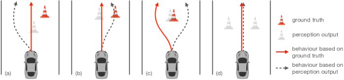
Figure 1: Illustration of behaviour change versus driving cost. The change in AV behaviour due to a perception error is not always correlated to the cost of consequence. In (a) the AV has to circumvent the erroneously perceived cone by making a large detour. While in (b) the AV only needs to make a slight detour to the right, yet it inevitably hits the cone. In this case, although the behaviour change is far less than that of (a), the consequence is significantly worse (‘hitting an object’ versus ‘making a large detour’). In (c) the consequence of either way is indifferent to the AV moving forward, yet the change in behaviour is considerable in terms of the spatiotemporal motion. In (d), though two falsely detected cones are close to the AV on both sides when passing by without collision, the AV still decides to maintain the same motion as in the ground truth case. In this scenario, the AV’s final behaviour remains the same regardless of the perception error, yet the cost of passing by two close obstacles already changes the planning process, which cannot be captured by the metrics that only look at the AV behaviour or planning result.

Recently, the community has begun to approach this problem with some initial efforts (Sun et al., 2020; Philion et al., 2020; Deng et al., 2021; Ivanovic & Pavone, 2022). Despite encouraging results, these preliminary solutions only address certain aspects of the problem, either implicitly relying on weak correlation between behaviour change and driving cost (Philion et al., 2020), inferring the holistic cost via local properties (Ivanovic & Pavone, 2022), or at coarse levels (Sun et al., 2020). In this work, we propose a principled and universal framework to quantify how noise in perception input affects AV planning. This is achieved by explicitly analysing the planning process in the context of expected utility maximisation (Osborne & Rubinstein, 1994), and evaluating the change in the utility function critical to the AV reasoning subject to input perception errors. We show that, under some practical conditions (Section 3.3), the planning process can be formulated as an optimisation problem with a linear objective function in a Hilbert space, where the utility to optimise is the inner product of an action-wise utility function and the world state distribution represented by perception. This geometric interpretation reveals many natural and insightful properties of the problem. For instance, any input error can be decomposed into two components: one does not affect the utility comparison (planning-invariant error), and the other one directly changes the planning problem (planning-critical error). Based on this novel insight, we derive a metric to quantify the consequence of a perception error in changing the planning process.

We want to emphasise the necessity of understanding the impacts of perception errors on an autonomous driving system via the planning process, rather than solely from the final result (i.e. the AV behaviour, or the trajectory output from the planner), as proposed by previous works (Philion et al., 2020). This results from the fact that the final planning result does not necessarily reflect how AVs evaluate the situation, reason with the environment, and assess the costs of actions. In fact, the correlation between behaviour change and the actual consequence is weak, or even negative in many common cases, as illustrated in Figure 1. In addition, most works implicitly or explicitly integrate a priori knowledge of the consequences of perception errors into the metric design. The complexity of such impact on autonomous driving, however, is far beyond handcrafted rules, defeating their purposes despite tremendous amounts of manual efforts. For instance, Deng et al. (2021) assume that the severity of an error should be weighted proportional to the reciprocal of its cubed Manhattan distance to the AV, regardless of its position relative to the latter. These presumptions, without convincing justification, could introduce biases that conceal crucial facts for evaluation purposes (see Section 5.2.2 for an example). In contrast, we make few such assumptions and solely rely on the planning process to infer the error consequence in a completely unbiased fashion, which enables our solution to capture many critical or subtle cases. In this regard, the core principle of our design resembles the philosophical concept of transcendental idealism proposed by Immanuel Kant in his classical work Critique of Pure Reason (Kant, 1781), which argues that, due to the limitation of the observer’s sensibility, the cognition of external objects is processed never as they are per se, but via the cognitive faculties and subject to the interpretation of the observer’s experience. For the same reason, the properties (e.g. ignorability, impact) of a perception error (an external object) ipso facto should be understood through the corresponding disturbance it causes to the AV planner (the observer) and measured by the extra loss incurred from the planning viewpoint, which gives the name to our framework: transcendental idealism of planner (TIP). Our code is available at https://github.com/qcraftai/tip.

2 Literature Review

Metrics for AV Perception Evaluation. Recent works aimed to assess the performance of perception from the autonomous driving system viewpoint mostly approach the problem in heuristic ways. Multiple heterogeneous detection metrics are directly combined to produce a single score for detector evaluation in the popular nuScenes benchmark (Caesar et al., 2020). Considering neural planners, Philion et al. (2020) implicitly hypothesise that consequences of perception errors on driving are directly correlated to the change in the planned spatiotemporal trajectories of an AV, and propose the planning KL-divergence (PKL) to measure the impact. While intuitive, it fails to incorporate the context of the environment and does not precisely reflect the real cost of perception noises in many common traffic scenarios. To address the specific problem of object representation, Deng et al. (2021) study how object shapes can affect autonomous driving and devise the support distance error (SDE) to quantify the effect. In another recent work, Ivanovic & Pavone (2022) look into the planning process and employ sensitivity as a probe of the input signal’s contribution to AV behaviour. This, however, only leverages local properties of differentiable cost functions to infer global results. In comparison, our approach systematically captures the global properties of the planning process and applies to more general cases. For convenience, the comparison of these metrics is summarised in Appendix D.

Planning for Autonomous Vehicles. In this work, we consider both behavioural decision making and motion planning as the planning process, which generates the vehicle behaviour for the controller to execute given the observation up to the planning time. There is a rich literature to address this fundamental problem for AVs, which can be roughly categorised into utility-based and utility-free methods. The former typically relies on a utility function to encode the predefined goals and strives for the optimal behaviour to accomplish the maximum return, via solving an optimisation problem with an explicit cost function manually engineered or learnt to guide vehicle trajectory generation (Buehler et al., 2009; Werling et al., 2010; Paden et al., 2016; Fan et al., 2018; Ajanovic et al., 2018), searching for the action policy with best reward return in the reinforcement learning framework (Kuefler et al., 2017; Schwarting et al., 2018; Kendall et al., 2019; Bronstein et al., 2022), etc.  The latter learns to drive by directly mapping input signals (raw or processed sensor data) into AV behaviours or vehicle control commands by leveraging deep learning from massive data (Bojarski et al., 2016; Guez et al., 2019; Grigorescu et al., 2020) as an alternative, which has attracted increasing attention from the research community recently. In spite of some promising results, nontrivial challenges still remain for this paradigm. For instance, behaviour cloning (Muller et al., 2005; Bansal et al., 2019; Prakash et al., 2021), one of the most popular strategies along this line, seeks to approach the human driving capability by learning from a large corpus of driving records available from human daily driving activities. Besides the considerable demand for supervised driving experiences to cover as many rare situations as possible for reliability, it suffers from generalisation issues by domain shift between training and deployment (Codevilla et al., 2019; Haan et al., 2019), as well as the inability, due to its open-loop learning nature, to infer long-term interaction between the AV and the environment (Zhang et al., 2022), a critical merit for handling complex traffic situations. In this work, we aim to exploit the properties of AV planners with explicit rewarding mechanisms to shed light on the impacts of perception noise on this process, and focus on utility-based planning.

3 Planning as Expected Utility Maximisation

To introduce our approach, we first present preliminary math basics to facilitate discussion, then review the expected utility maximisation as the optimal AV action framework, followed by its interpretation in a Hilbert space, based on which our metric for perception evaluation is derived.

3.1 Preliminaries

Unless otherwise specified explicitly, all notation follows the standardised one in (Goodfellow et al., 2016). A probability space $\{\Phi,\mathcal{F},\mathcal{P}\}$ is defined by a sample space $\Phi$, an event space $\mathcal{F}$ (a $\sigma$-algebra on $\Phi$), and a Borel probability measure $\mathcal{P}$ on $\mathcal{F}$. A random variable $X\mathrel{\mathop{\mathchar 58\relax}}\Phi\rightarrow\mathbb{R}^{d}$ ($d\in\mathbb{N}$) is induced from $\{\Phi,\mathcal{F},\mathcal{P}\}$ with distribution function ${F}_{X}(x)$. When absolutely continuous, ${F}_{X}(x)=\int_{-\infty}^{x}f_{X}(t)\operatorname{d\!}t$, where $f_{X}(x)$ is the probability density function (PDF). $L^{2}({\mathcal{X}},\rho)$ denotes the space of square-integrable functions, and $\rho$ is a Lebesgue measure accordingly. A Hilbert space ${\mathcal{H}}=({\mathcal{T}},\left\langle\cdot,\cdot\right\rangle)$ is defined on a complete space ${\mathcal{T}}$ with inner-product $\left\langle\cdot,\cdot\right\rangle_{\mathcal{H}}$ and induced norm $\mathinner{\!\left\lVert\cdot\right\rVert}_{\mathcal{H}}$. Let $S\subset{\mathcal{H}}$ be a subspace of ${\mathcal{H}}$, $S^{\perp}=\{x\in{\mathcal{H}}|\left\langle x,y\right\rangle,\forall y\in S\}$ is the orthogonal complement of $S$ (i.e. the set of all vectors orthogonal to $S$). $\textup{span}(S)$ is the linear span of a set $S$. $n_{v}\coloneqq{v}/{\mathinner{\!\left\lVert v\right\rVert}}$ is an element of unit length in a normed vector space by normalising element $v$.

3.2 Autonomous Vehicles as Rational Agents

An AV is an intelligent agent that aims to accomplish some predefined goals in an interactive and uncertain environment. It is constantly faced with planning problems in the dynamic surroundings, and the quality of planning determines how well the goals can be achieved. By the classical expected utility maximisation (EUM) theory (Osborne & Rubinstein, 1994), at any given time $t$, an AV aims to achieve the maximum expected reward, defined by the utility function ${U}$, via execution of the optimal action ${a}^{*}_{t}$ such that

$$\vspace{-0.5mm}{a}^{*}_{t}=\operatorname*{arg\,max}\nolimits_{{a}\in\mathcal{D}_{{a},t}}~{}\mathbb{E}\left[{U}(S_{t},{a})\right],$$ (1)

where $\mathcal{D}_{{a},t}$ is the set of all feasible AV actions at time $t$; ${s}\in{\mathcal{S}}$ is the state random variable at time $t$ with distribution function ${F}_{S_{t}}({s})$ in the world state space ${\mathcal{S}}$; and

$$EU({F}_{S_{t}},a)\coloneqq\mathbb{E}\left[{U}(S_{t},{a})\right]=\scalebox{1.3}{$\int$}_{{s}\in{\mathcal{S}}}~{}{U}({s},{a})\operatorname{d\!}{F}_{S_{t}}({s}).$$

Intuitively, the utility function encodes the goal or reward the AV is supposed to achieve (e.g. reaching a destination in time, avoiding collision with other objects). ${F}_{S_{t}}({s})$ captures uncertainty about the stochastic environment given all world knowledge and historical observations up to $t$, which are estimated by modules like localisation and perception (Luo et al., 2021a, b). Architectures of many modern AV planners still follow the concept of this classical framework as its variants (Paden et al., 2016; Fan et al., 2018; Sadat et al., 2020; Bronstein et al., 2022; Zhang et al., 2022).

3.3 Expected Utility Maximisation in Hilbert Space

To gain some insights into the expected utility of (1) and how input noises affect the planning process, we introduce an interpretation in the Hilbert space to leverage geometric tools available from linear algebra. We first establish the conditions under which a probability measure can be embedded into a Hilbert space, followed by the interpretation of EUM from a geometric perspective in Section 4. For brevity, all proofs are left in Appendix G.

Theorem 3.1 (Probability Measure Embeddings in the Hilbert Space).

Let $\{{\mathcal{X}},{\mathtt{d}}\}$ be a compact metric space with ${\mathtt{d}}$ as the metric function, ${p}$ be a Borel probability measure on ${\mathcal{X}}$, and $X$ be a random variable on ${\mathcal{X}}$ with distribution function ${F}_{X}(x)$. If ${F}_{X}(x)$ is absolutely continuous and the density function $f_{X}$ is square-integrable, i.e. $f_{X}\in L^{2}$, then there exists a unique element$\mu_{p}\in{\mathcal{H}}$ such that

$$\mathbb{E}_{X}\left[g(x)\right]=\left\langle{\mu_{p}},g\right\rangle_{{\mathcal{H}}},~{}\forall g\in{\mathcal{H}},\vspace{-1mm}$$ (2)

where element $\mu_{p}$ denotes the embedding of probability measure ${p}$ in the Hilbert space ${\mathcal{H}}=(L^{2},\left\langle\cdot,\cdot\right\rangle)$, with the inner product given by

$$\left\langle g,h\right\rangle_{{\mathcal{H}}}\coloneqq\scalebox{1.1}{$\int$}_{x}~{}g(x)h(x)\rho(\operatorname{d\!}x).\vspace{-1mm}$$

The critical condition of ${F}_{X}(x)$ being absolutely continuous with a square-integrable density function $f_{X}$ in Theorem 3.1 is general and includes many common distributions as special cases (see Appendix F). The mapping from probability measures of continuous random variables to ${\mathcal{H}}$ established by Theorem 3.1 is also injective by the following result.

Theorem 3.2 (Injection of Probability Measure Embeddings).

Let ${p}$ and ${q}$ be two Borel probability measures defined on a compact metric space $\{{\mathcal{X}},{\mathtt{d}}\}$ with absolutely continuous distribution functions, then ${p}={q}$ almost everywhere if and only if $\mu_{p}=\mu_{q}$, where $\mu_{p}$ and $\mu_{q}$ are the embeddings of ${p}$ and ${q}$ in ${\mathcal{H}}$, respectively.

A similar result for mixed distributions is also available in Theorem G.4 for deterministic perception results (treated as Dirac delta distributions) and guarantees that following discussion on probabilistic perception results can be readily extended to these cases. Under the conditions in the aforementioned results, the EUM of (1) can be rewritten as

$${a}^{*}=\operatorname*{arg\,max}\limits_{{a}\in\mathcal{D}_{{a}}}\mathbb{E}_{{p}({s})}\left[{U}({s},{a})\right]=\operatorname*{arg\,max}\limits_{{a}\in\mathcal{D}_{{a}}}\left\langle{\mu_{p}},{U}_{a}\right\rangle_{{\mathcal{H}}}.$$ (3)

Given this injective correspondence between ${p}$ and $\mu_{p}$, we can leverage many tools in algebra (e.g. inner product, orthogonality, projection) to analyse the impact of perception errors on AV planning via the EUM in ${\mathcal{H}}$, where the topological structure is exclusively determined by its inner product.

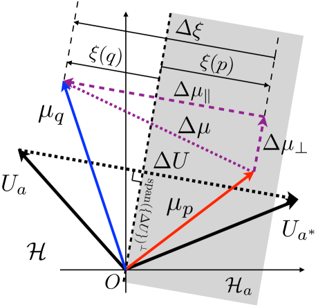
Figure 2: Illustration of EUM in ${\mathcal{H}}$. $\Delta{U}={U}_{{a}^{*}}-{U}_{{a}}$ defines the behaviour direction; $\xi$ is the preference score; $\mu_{p}$ and $\mu_{q}$ are the embeddings of the ground truth and perception results, respectively; $\Delta\mu$ is the perception error, which is decomposed into the planning-critical error (PCE) $\Delta\mu_{\parallel}$, and the planning-invariant error (PIE) $\Delta\mu_{\perp}$; and the shaded area corresponds to ${\mathcal{H}}_{a}$. Note that ${\footnotesize\langle{\Delta\mu_{\parallel}},{\Delta{U}}\rangle}<0$.

4 Perception Evaluation via AV Planning

In this section, we derive the effect of perception errors on planning via the theoretical foundation established in Section 3. Without loss of generality, we assume that the perception module is the only source for world state estimation in the following discussion.

4.1 Breakdown of Perception Errors

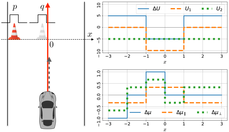
Figure 3: An example of PCE $\Delta\mu_{\parallel}$ and PIE $\Delta\mu_{\perp}$. An AV is moving forward on a $6$m-wide road; there is a cone in front on a line across the road (the $x$ axis). The ground truth distribution of the cone location ${p}$ is $\mathcal{U}_{[-3,-2]}$, a uniform distribution with support $[-3,-2]$, while the perception predicts its location distribution ${q}$ to be $\mathcal{U}_{[-1,0]}$. The 2m-wide AV has two action options: (i) to keep moving forward (${a}^{*}$, the solid line with an arrowhead), and the utility function is ${U}_{1}(x)=-10\cdot\bm{1}{x\in[-1,1]}$ with $x$ being the position of the cone (only large loss for collision with the cone); (ii) to come to a full stop before the line via hard braking (${a}$, the dashed line with an arrowhead), and the utility function is a constant ${U}_{2}(x)=-5$ (loss of hard braking is consistent regardless of the cone position). Note that $\Delta\mu_{\parallel}$ is of the same shape as $\Delta{U}={U}_{1}-{U}_{2}$ (up to a negative constant), and $\left\langle\Delta{U},\Delta\mu_{\perp}\right\rangle_{{\mathcal{H}}}=0$. In this example, PCE accounts for 33.3% of the error energy, while PIE for 66.6%. See Figure 8(b) for another case where ${\footnotesize\left\langle\Delta\mu,\Delta{U}\right\rangle_{{\mathcal{H}}}>0}$.

Consider a general case where the candidate action set is $\mathcal{D}_{a}=\{{a}_{i}\}$, and each action is associated with a distinct utility function ${U}({s},{a}_{i})\in{\mathcal{H}}$ such that, $\forall{a}_{i},{a}_{j}\in\mathcal{D}_{a}$,

$$\mathinner{\!\left\lVert{U}({s},{a}_{i})-{U}({s},{a}_{j})\right\rVert}_{\mathcal{H}}>0\Leftrightarrow{a}_{i}\neq{a}_{j}.$$

Let ${a}^{*}$ be the optimal action per EUM of (3) given the ground truth world state distribution ${p}({s})$. For any ${a}\neq{a}^{*}$, $\Delta{U}({{a}^{*}},{a})={U}_{{a}^{*}}-{U}_{{a}}$; the planning half-space in ${\mathcal{H}}$ is

$${\mathcal{H}}_{{a}}\coloneqq\{f|\left\langle f,\Delta{U}({{a}^{*}},{a})\right\rangle_{{\mathcal{H}}}>0,f\in{\mathcal{H}}\}.$$

Given the perception result ${q}({s})$, ${a}^{*}$ is preferred over ${a}$ by EUM if and only if $\mu_{q}\in{\mathcal{H}}_{{a}}$, i.e.

$$\xi({q};{a}^{*},{a})>0\vspace{-2mm}$$ (4)

with

$$\xi({q};\alpha,\beta)\coloneqq\left\langle{\mu_{q}},\Delta{U}({\alpha},\beta)\right\rangle=EU({q},\alpha)-EU({q},\beta)$$ (5)

denoting the $\alpha$-$\beta$ preference score given ${q}$ ($\forall\alpha,\beta\in\mathcal{D}_{a}$), which exclusively decides the result of EUM. As illustrated in Figure 2, the planning result remains ${a}^{*}$ if and only if

$$\mu_{q}\in\scalebox{1.0}{$\bigcap\nolimits_{{a}\in\mathcal{D}_{a}/\{{a}^{*}\}}$}{\mathcal{H}}_{{a}}.$$

When ${q}({s})$ is erroneous (i.e. $\mathinner{\!\left\lVert\mu_{q}-\mu_{p}\right\rVert}_{\mathcal{H}}>0$), the preference score of (4) may be affected, i.e. $\xi({q};{a}^{*},{a})\neq\xi({p};{a}^{*},{a})$, so is the result by EUM. To understand how error $\Delta\mu=\mu_{q}-\mu_{p}$ changes the result of EUM, we further decompose $\Delta\mu$ into two orthogonal components:

$$\Delta\mu=\mu_{q}-\mu_{p}={\Delta\mu}_{\parallel}+{\Delta\mu}_{\perp},\vspace{-2mm}$$ (6)

where

$${\Delta\mu}_{\parallel}=\left\langle\Delta\mu,n_{\Delta{U}}\right\rangle_{{\mathcal{H}}}n_{\Delta{U}}=\frac{\left\langle\Delta\mu,\Delta{U}\right\rangle_{{\mathcal{H}}}}{\mathinner{\!\left\lVert\Delta{U}\right\rVert}_{\mathcal{H}}^{2}}\Delta{U}$$ (7)

is the projection of $\Delta\mu$ onto unit vector $n_{\Delta{U}}$ (denoted behaviour direction), and ${\Delta\mu}_{\perp}\in\textup{span}(\{{\Delta{U}}\})^{\perp}$ is the projection of ${\Delta\mu}$ onto the orthogonal complement of the subspace spanned by the behaviour direction, i.e. $\left\langle\Delta\mu_{\perp},\Delta{U}\right\rangle_{{\mathcal{H}}}=0$. In the presence of error $\Delta\mu$, as illustrated in Figure 2 and Figure 8(a), the change in preference score of (4) is only determined by ${\Delta\mu}_{\parallel}$:

$$\Delta\xi({a}^{*},{a};{q},{p})= ~{}\xi({q};{a}^{*},{a})-\xi({p};{a}^{*},{a})$$ (8)

$$= ~{}{\footnotesize\left\langle\Delta\mu,\Delta{U}\right\rangle_{{\mathcal{H}}}}$$

$$= ~{}{\footnotesize\langle{\Delta\mu_{\parallel}},{\Delta{U}}\rangle}_{{\mathcal{H}}}.$$

For this reason, we denote $\Delta\mu_{\parallel}$ as the planning-critical error (PCE), and $\Delta\mu_{\perp}$ as the planning-invariant error (PIE) (see Figure 3 and Appendix A for more discussion). The observation reveals two pivotal facts: (i) not all errors in perception (world state estimation) are of equivalent impact on planning, and the subspace $\textup{span}(\{{\Delta{U}}\})^{\perp}$ contains all errors that do not affect EUM at all; (ii) errors in subspace $\textup{span}(\{{\Delta{U}}\})$ either negatively affect planning (if ${\footnotesize\left\langle\Delta\mu,\Delta{U}\right\rangle<0}$), or even favour the optimal action ${a}^{*}$ (if ${\footnotesize\left\langle\Delta\mu,\Delta{U}\right\rangle>0}$). Intuitively, $\Delta\xi$ measures the impact of perception error $\Delta\mu$ on the decision between ${a}^{*}$ and ${a}$.

4.2 Estimation of Preference Score $\xi$

In practice, combining (5) and (8), evaluating the impact of a perception error $\Delta\mu$ on ${a}^{*}$-${a}$ decision is reduced to

$$\begin{split}\Delta\xi({a}^{*},~{}&{a};~{}{q},~{}{p})\\ =~{}&\mathbb{E}_{{q}({s})}\left[{U}({s},{a}^{*})\right]-\mathbb{E}_{{p}({s})}\left[{U}({s},{a}^{*})\right]\\ ~{}&-\mathbb{E}_{{q}({s})}\left[{U}({s},{a})\right]+\mathbb{E}_{{p}({s})}\left[{U}({s},{a})\right].\end{split}$$ (9)

Computing these expectations in analytical forms typically requires strong assumptions on the forms of both utility and distribution functions for precise results, or variational methods for approximation (Bishop, 2006), which limits representation capacity or accuracy. For maximum flexibility, we resort to numerical methods by estimating the expected utilities from finite-size samples of world states, and show that the solution is both statistically consistent and uniformly efficient under practical conditions. Specifically, for a fixed action ${a}$, given an i.i.d. sample of the utilities $\{U(S_{i},{a})\}_{i=1}^{n}$ with $S_{i}$ drawn from ${p}_{S}({s})$, an unbiased estimator of the expected utility via U-statistics is

$$EU_{a}=\frac{1}{n}\sum\nolimits_{i=1}^{n}U(S_{i},{a}).$$ (10)

A fast convergence rate via the uniform bound can be achieved by the following observation for the estimator.

Theorem 4.1 (Exponential Convergence Rate).

If there exists an $M\in\mathbb{R}$ such that $\mathinner{\!\left\lvert{U}(S,{a})\right\rvert}<M$ almost surely, then for $EU_{a}$ of (10), $\forall\varepsilon>0$,

$$\textup{Pr}\Big{(}\mathinner{\!\left\lvert EU_{a}-\mathbb{E}\left[{U}(S,{a})\right]\right\rvert}>\varepsilon\Big{)}<2\exp\Big{(}-\frac{n\varepsilon^{2}}{2L}\Big{)},$$ (11)

where $L=\min\Big{(}M^{2},\textup{Var}\left({U}(S,{a})\right)+\frac{M\varepsilon}{3}\Big{)}$.

Note that, the condition of Theorem 4.1, assigning finite values to the utility in the worst or best cases, is a practical necessity even for life-related scenarios (Russell & Norvig, 2020, Chapter 16.3). The exponential convergence rate of $O(e^{-n})$ provided by Theorem 4.1 is significant: it depends on (i) neither the dimensionality of the original state space ${\mathcal{S}}$, i.e. the curse of dimensionality is not invoked (Wasserman, 2010), nor (ii) the distribution and utility functions, i.e. ${U}(S,{a})$ and ${p}_{S}({s})$ can take any arbitrary forms.

Input : A query perception sequence ${{q}(\{{s}_{t}\}_{t=-\tau}^{0})}$, the ground truth ${{p}(\{{s}_{t}\}_{t=-\tau}^{0})}$, sample size $n$

Output : TIP score $\mathscr{I}({q},{p};{U},\mathcal{D}_{a})$

Get the candidate action set $\mathcal{D}_{{a},{p}}$ and the optimal action ${a}^{*}\in\mathcal{D}_{{a},{p}}$ from the planner with the ground truth ${p}$

Get the candidate action set $\mathcal{D}_{{a},{q}}$ from the planner with the query perception input ${q}$

$\mathcal{D}_{a}\leftarrow\mathcal{D}_{{a},{p}}\cup\mathcal{D}_{{a},{q}}$

foreach ${a}\in\mathcal{D}_{a}$ do

       $\{{s}_{{p}}^{(i)}\}_{i=1}^{n}$ $\leftarrow$ $n$ i.i.d. observations from ${p}$

      $\{{s}_{{q}}^{(i)}\}_{i=1}^{n}$ $\leftarrow$ $n$ i.i.d. observations from ${q}$

$${\Delta\xi}_{a}\leftarrow\frac{1}{n}\sum\nolimits_{i=1}^{n} ~{}\Big{[}{U}({s}_{{q}}^{(i)},{a}^{*})-{U}({s}_{{q}}^{(i)},{a})$$

$$~{}~{}~{}~{}-{U}({s}_{{p}}^{(i)},{a}^{*})+{U}({s}_{{p}}^{(i)},{a})\Big{]}$$

end foreach

$\mathscr{I}({q},{p};{U},\mathcal{D}_{a})\leftarrow\min\nolimits_{{a}\in\mathcal{D}_{{a}}}{\Delta\xi}_{a}$

Algorithm 1 TIP Score Computation

4.3 Perception Error Impact on Planning by TIP

Given the consequence of a perception error evaluated on an action ${a}$ in (8) , its impact on AV planning is defined as the maximum reduction of preference scores among all candidate actions in $\mathcal{D}_{a}$:

$$\mathscr{I}({q},{p};{U},\mathcal{D}_{{a}})\coloneqq\min\nolimits_{{a}\in\mathcal{D}_{{a}}}\Delta\xi({a}^{*},{a};{q},{p})\leqslant 0.\vspace{-2mm}$$ (12)

This leads to the optimal sensitivity to the worst case. Other alternatives, nevertheless, are also possible for different trade-offs between selectivity and invariance, e.g. means, top $k$ percentiles (Li & Vasconcelos, 2015). In our case, the action set contains spatiotemporal trajectories the planner considers in all phrases during the whole planning process (see Appendix C for more details). To facilitate the understanding of our approach, the pseudocode is provided in Algorithm 1, which sketches the basic routine to compute the TIP score of a perception input sequence ${q}(\{{s}_{t}\}_{t=-\tau}^{0})$ from $t=-\tau$ to $t=0$ for planning at $t=0$.

It should be noted that, once the planner utility function is established for scenario-independent deployment, TIP score evaluation is a parameter-free process, and results are readily comparable across different scenarios. This advantage is in contrast to other handcrafted metrics like NDS or SDE-APD, which require either manual specification (Caesar et al., 2020) or calibration (Deng et al., 2021), thus may behave inconsistently inside and outside the intended noise dynamic range, as will be seen in Section 5.2.1.

5 Empirical Study

In this section, we evaluate how TIP works empirically via extensive qualitative and quantitative experiments conducted on both synthetic and real data.

5.1 Basic Settings

All AVs used in the experiments are based on the same type of regular passenger vehicles. The planner deployed on the AVs consists of various sub-modules of routing, object motion forecasting, cost generation, path finder, and trajectory optimisation. At each planning time, these sub-modules analyse the environment and input history to establish the target utility function ${U}(\cdot,{s})$ for final trajectory optimisation. The path finder then provides multiple initial paths as candidates for path-wise trajectory optimisation, and the final choice is determined by a utility decider. The goals the planner strives to achieve include motion smoothness, traffic rule compliance, safety, progress to the destination, etc. The final output trajectory is subject to independent Gaussian noise at each time step to account for control inaccuracy. The planner has been extensively verified via rigorous road tests in major cities with millions of population (see Appendix C for more details). Note that, while we adopt a planner following the popular module-based architecture to evaluate the proposed metric in this work, it can also be readily applied to other utility-based alternatives, e.g. planners learnt via the imitation learning (Kuefler et al., 2017), Markov decision process (Zhang et al., 2022), or with trajectory density modelling (Bronstein et al., 2022).

All experiments are implemented in scenarios as the standard protocol in autonomous driving (Riedmaier et al., 2020). The scenarios used are collected from real world road tests (more details in Appendix B). We consider the planning problem at a particular frame in a scenario at a time, and evaluate the utility of an action (a spatiotemporal trajectory the AV executes) for the next three seconds, following the basic setup of (Philion et al., 2020). For comparison, three baselines are adopted from the spectrum of perception metrics: (i) at the conventional end, nuScenes dataset score (NDS) combines several traditional scoring results for 3D object detection into a single performance measure (Caesar et al., 2020), (ii) SDE average precision distance-weighted (SDE-APD) focuses more on detections near the AV in an ego-centric fashion (Deng et al., 2021), and (iii) PKL (Philion et al., 2020) serves as the representative of AV behaviour-based metrics in the literature.

5.2 Results on Synthetic Data

In the first set of experiments, we aim to gain some understanding of various metrics in reaction to common types of perception noises. A dataset is synthesised from our curated road test scenarios by adding controlled noise to the 3D object ground truth of vehicles, to enable clear observation of the sensitivity of metrics to specific perception error types. For this, 1000 5s-long scenarios are assembled, with the number of objects per scene between 30 and 500 and an average AV speed of 5m/s or higher. The ground truth is annotated by professionally trained human operators. All objects in the scenario are labelled with location, heading, category, and bounding box from 3D point clouds recorded by onboard LiDAR sensors during road tests.

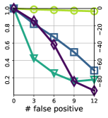
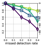
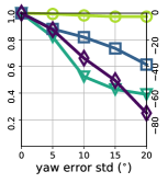
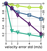
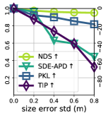
Figure 4: Comparison of metrics on different cases of synthetic noise. The left (right) vertical axes are for NDS and SDE-APD (PKL and TIP).

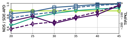
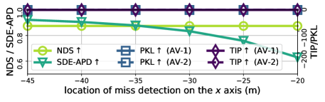
Figure 5: Metrics for AVs of different driving styles. On the $x$-axis are (i) a miss detected stationary obstacle; (ii) another stationary vehicle at $x$=50; and (iii) an AV at $x$=0 moving along the +$x$ direction at 14m/s. AV-1 (‘jerk-averse’) is optimised for driving comfort with braking capped at -4m/s², while AV-2 (‘collision-averse’) is for safety, which can brake as much as -6m/s². The stopping distance is around 30m and 20m, respectively.

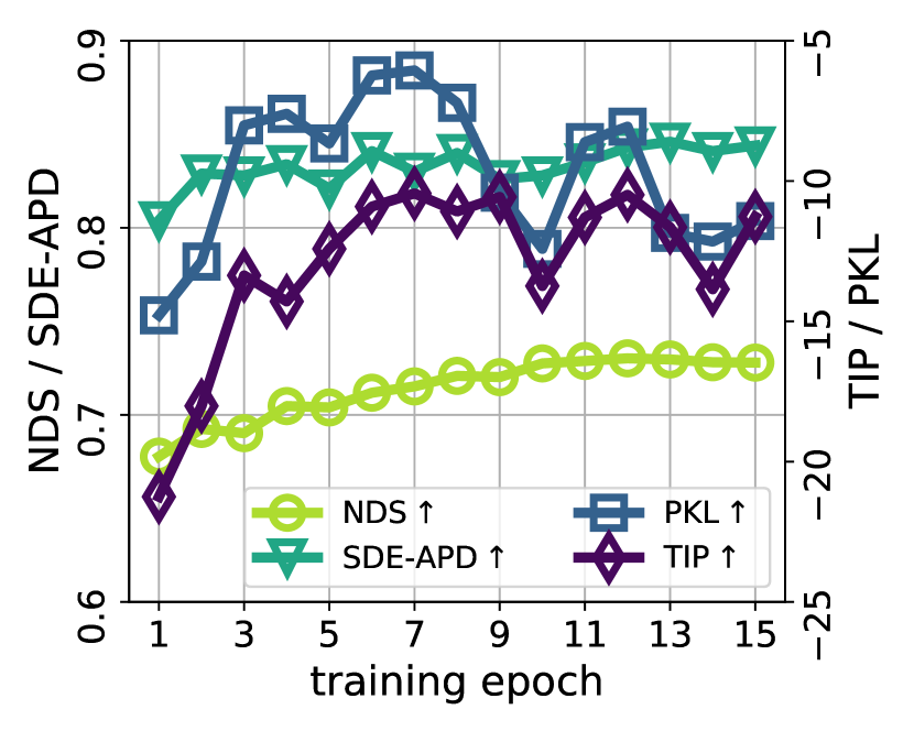
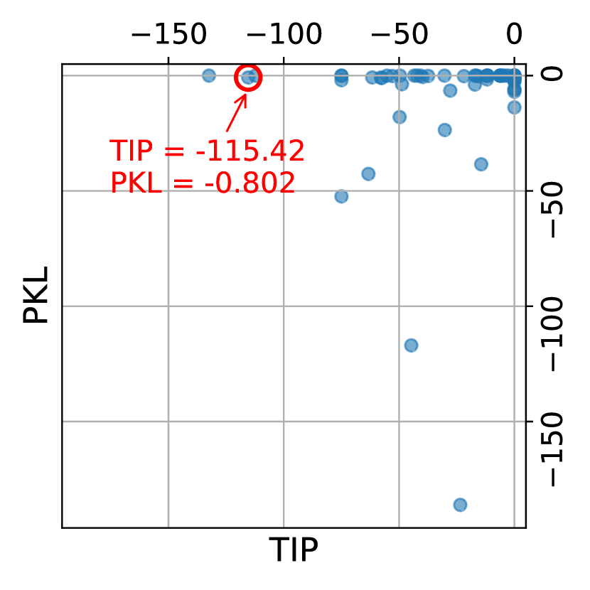
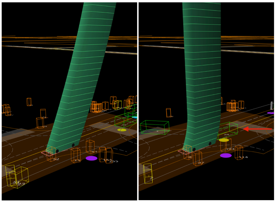
Figure 6: Comparison of metrics on real data. Left: metrics on different checkpoints during training. Middle: scatter plot of impacts of perception noise measured by TIP and PKL. Note the number of data points close to the $x$-axis (PKL = 0), which correspond to critical errors in planning due to the perception noise captured by TIP yet missed by PKL since the AV behaviours are similar with and without the noise. Right (best viewed in colour): the first one is the ground truth with the corresponding AV behaviour (the spatiotemporal trajectory illustrated by the green tube with the $z$-axis as the temporal dimension); the second one shows an outrageous error of a false positive (pointed to by the red arrow), which causes a jerk of $-76.4$m/s³ while the typical limit is around $-1.0$m/s³ (Wang et al., 2018), despite a mild change in behaviour per PKL. PKL and TIP of this case are highlighted by the red circle in the middle scatter plot. See details in Appendix D.1.

5.2.1 Reaction to Different Types of Noise

In total, six types of errors are considered. The false positives are tested by adding ‘ghost’ vehicles scattered within a 70m-by-30m box centred at the AV, with motion properties randomly perturbed from it. The miss detection is created by removing objects from the ground truth randomly with a certain probability (i.e. miss detection rate). Other noises involving location, yaw, velocity and size are sampled from zero-mean Gaussian with different variances and added to corresponding properties of ground truth. The results are shown in Figure 4. While all metrics negatively correlate with all six types of noises, NDS saturates in some cases (e.g. velocity) due to its design. SDE-APD, also handcrafted with parameters calibrated from particular data sources, exhibits varying sensitivity at different noise levels, especially for the velocity (computed by SDE-APD@$t$=1s), as the default matching threshold 0.2m is easily overwhelmed by speed noise larger than 1m/s. In comparison, planner-centric metrics like PKL and TIP, with little manual engineering involved, render more consistent sensitivity across the whole dynamic range of different noises.

5.2.2 Case Study with Different Planners

We further investigate the behaviour of TIP with different planner settings. In a typical miss detection scenario, we remove a stationary vehicle in front of or behind an AV moving forward, as shown in Figure 5. Both SDE-APD and PKL consider closer miss detections, under any circumstances, worse than further ones. TIP, however, predicts that AV-1 regards the one at 30m as the worst: the collision is inevitable even if the obstacles at 20m and 25m are detected; yet the miss detection at 30m leads to a collision that could have been (barely) avoided otherwise. In contrast, no other metrics provide insights at this level of subtlety. This demonstrates the superior resolution of TIP in identifying critical events from the planning perspective that would have been missed by all other baselines (especially SDE-APD, which explicitly incorporates the belief that the closer the miss detection is, the worse it is per se). On the other hand, when the miss detection happens behind the AV, both TIP and PKL ignore its impact. NDS and SDE-APD, however, fail to distinguish errors on both sides of the AV, due to their spatial or directional homogeneity by design (note the symmetry of them in both directions of the $x$-axis).

5.3 Results on Real Data

In the second set of experiments, we study the results from the real perception module deployed on our AVs, which is exemplified by a 3D object detection network that predicts the class, location, heading, velocity and size of objects from LiDAR point clouds. TIP is independent of the specific detector and can be applied to various methods (Lang et al., 2019; Shi et al., 2020; Yin et al., 2021; Li et al., 2023). We develop an effective and efficient pillar-based network, which is trained on 780K LiDAR sweeps using annotations of vehicle, pedestrian and cyclist with a detection range of [-67.2m, 124.8m]$\times$[-51.2m, 51.2m].

5.3.1 Training Checkpoints

A typical challenge in developing a perception model is to determine how much training is needed to reach a satisfactory level of performance. Conventional solutions require a variety of heterogeneous metrics to measure different aspects of an algorithm (e.g. mean average precision for detection, mean squared errors for motion properties). Recently, unified metrics like NDS (Caesar et al., 2020) are also proposed by manual engineering, which hardly confirm the driving quality improvement of a perception model change. In most cases, conclusions can only be made from large-scale real road tests, which are extremely costly (Wachenfeld & Winner, 2016; Åsljung et al., 2017).

We evaluate the performance of our 3D object detection model on the same test scenarios (without any artificial noise) as in Section 5.2 and compare the model output against the ground truth. The model is trained for 15 epochs, with results reported on the left of Figure 6. Unsurprisingly, NDS tends to increase as the training progresses and the final checkpoint models usually achieve the best performance since NDS combines the errors that are aligned with the loss functions optimised during training. When evaluated with the AV involved, however, the observation changes. SDE-APD implies that the training seems to struggle with improving results on close-by objects as the losses are dominated by a large number of far-away yet more challenging objects. From either behaviour or planning perspectives, TIP and PKL both indicate that the last checkpoint model is not among the best possible models during training. Instead, models somewhere in the middle of the training can provide better autonomous driving performance. Actually, neither TIP nor PKL is improved significantly beyond the 7th epoch, suggesting that early termination of training may be even more beneficial to driving. More importantly, we notice that TIP disagrees with PKL on scenarios across models of top performance, and there are quite some critical cases identified by TIP yet missed by PKL. The difference is illustrated in the middle of Figure 6 by the scatter plot of randomly sampled scenarios, where PKL is almost zero while TIP scores are nontrivial in many scenarios, suggesting the drastic impacts of perception errors on the planning process despite similar AV behaviours with or without these errors (see the example on the right of Figure 6 and others discussed in Appendix D.1).

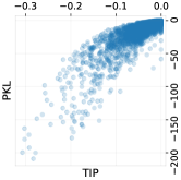
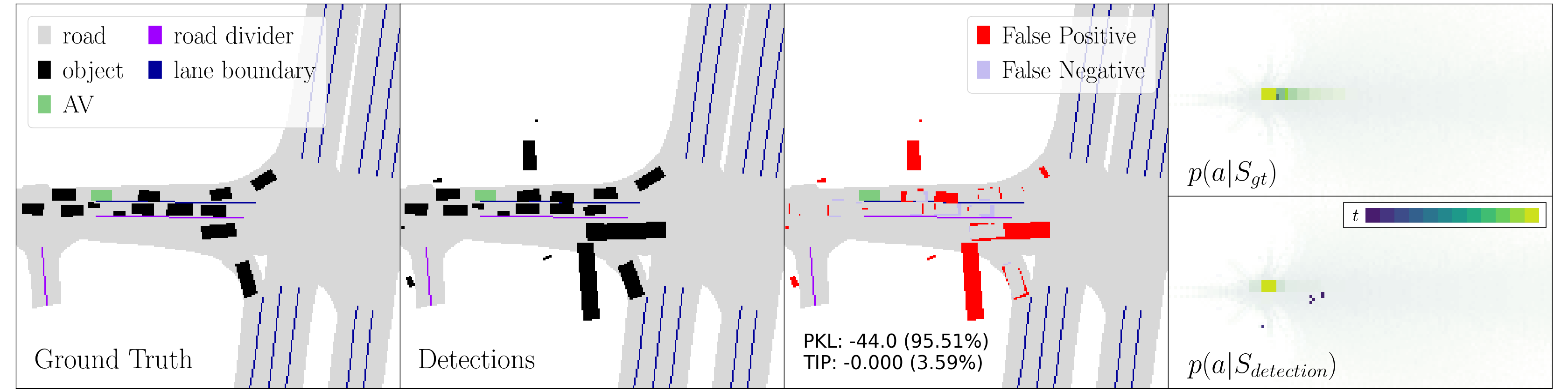
Figure 7: Results of CBGS detector on nuScenes validation set. Left: scatter plot of PKL and TIP scores (note that ranges of both metrics are different from previous experiments since the planners used are distinct). Middle and Right: a typical scenario where PKL deems a large impact on the planner from the perception noise yet TIP considers it insignificant (score percentiles in the whole dataset are also shown in parentheses). Ground truth, detector outputs, their difference, and planner outputs (AV location distributions over time with one solid colour indicating the most likely locations at one time step, which are not plotted to the numeric scale for visual saliency enhancement) are shown, respectively.

5.3.2 More Perception Models

Table 1: Comparison of different perception models.

Detector	NDS$\uparrow$	SDE-APD$\uparrow$	PKL$\uparrow$	TIP$\uparrow$
Pillar	0.730	0.843	-8.1	-10.5
PillarNeXt-1F	0.693	0.852	-9.2	-11.7
PillarNeXt-5F	0.744	0.878	-7.9	-9.1

Table 2: Metric favour rate$\uparrow$ by the subjective evaluation.

Metric	NDS	SDE-APD	PKL
TIP†	82%†vs.18%	66%†vs.34%	61%†vs.39%

To evaluate other 3D detectors, we implement two more models with the recent PillarNeXt (Li et al., 2023) as the basic detector. The first one (PillarNeXt-1F) uses the point cloud only from the current frame for prediction, while the second one (PillarNeXt-5F) leverages 5 consecutive frames around the current one. Results are reported in Table 1. Both models have better performance by SDE-APD. PillarNeXt-1F, however, fails to produce precise velocity from single-frame observation (not reflected by SDE-APD), leading to an inferior performance by the other three metrics. PillarNeXt-5F delivers overall best results across all metrics, despite marginal gaps by PKL and NDS.

5.3.3 Subjective Evaluation

To further justify the soundness of the proposed approach on the scenario level, we also implement a set of subjective evaluations similar to that in (Philion et al., 2020). We collect 258 scenario pairs with actual perception noises and check whether TIP, PKL, SDE-APD or NDS disagree on the relative severity, i.e. one believes the perception error in scenario A is worse than that in scenario B while the other one thinks alternatively. These pairs of scenarios are compared by 10 human drivers to decide which is worse subjectively. The result reported in Table 2 suggests that human drivers side with TIP more over the other three baselines.

5.4 Application to Neural Planners

The proposed framework is also applicable to neural planners with implicitly derived behaviour cost or likelihood functions for inference such as (Bansal et al., 2019; Zeng et al., 2019; Philion et al., 2020). For this, we implement TIP scoring on the neural planner from (Philion et al., 2020), where the output trajectory PDF ${p}({a}|S)$ is adopted in lieu of the utility function ${U}(S,{a})$ for TIP. Given any perception input, the planner produces a distribution of AV future actions ${p}({a}|S)$ and the one with the highest probability (density) is chosen as the AV behaviour ${a}^{*}=\operatorname*{arg\,max}_{a}{p}({a}|S)$.

Under this setting, PKL and TIP evaluate the impact of perception noise on the planner with different nuances, as reflected by the results shown in Figure 7, where the PKL and TIP scores for the CBGS detector (Zhu et al., 2019) on the validation set of nuScenes 3D object detection task (Caesar et al., 2020) are presented. The former considers feasible actions of all road vehicles and aggregates the difference between the action distribution given ground truth and perception inputs across the whole action space. The latter, in contrast, focuses on the optimal action ${a}^{*}$ the AV actually executes (given the ground truth input and subject to kinetic and kinematic constraints) and evaluates the reduction in AV’s favourability on ${a}^{*}$ over any other candidate actions given the two different inputs. Consequently, TIP captures a nontrivial number of scenarios where perception noises affect the behaviour of some general road vehicles but impact not necessarily that much on the AV per se. See Appendix E for more discussion.

6 Notes on Dependence on the Planner

The proposed framework relies on a planner’s reactions to input noises to evaluate perception, a prominent property for all planning-centric metrics (Philion et al., 2020; Ivanovic & Pavone, 2022). Due to this dependence on the planner, evaluation results of these metrics on the same perception input may change as the underlying planner varies. While not necessarily a drawback, it does incur some extra cost to ensure proper application of these metrics. Most importantly, the planner should be sufficiently verified before being deployed with the metrics for evaluation, either by validation on benchmarks (Philion et al., 2020), virtual simulation (Dosovitskiy et al., 2017), or real world road test as for our planner in Section 5.1. In addition, all interpretations of the result should be made in the specific context of the planner employed, and any observations are planner-bound, e.g. numeric scores from the same metric should only be compared against those from the same planner per se.

7 Conclusion

In this work, we have proposed TIP, a principled framework to evaluate perception from the planning perspective for autonomous driving. TIP explicitly exploits properties of utility-based planners and effectively identifies perception noises that may cause large planning changes in the context of expected utility maximisation. Extensive experiments on both synthetic and real data confirm that TIP is capable of distinguishing perception errors that would not be identified by the conventional and ego-centric metrics, or those exclusively focusing on behaviours output from the planner.

Appendix

Appendix A Planning-Critical Errors

When $n_{\Delta\mu_{\parallel}}=n_{\Delta{U}}$, the change in preference score $\Delta\xi({a}^{*},{a};{q},{p})$ of (8) is positive, suggesting that the difference between the expected reward by executing ${a}^{*}$ and that of ${a}$ is even larger with noisy perception input ${q}$ than with the ground truth ${p}$, i.e. the planner is even more confident in choosing ${a}^{*}$ over ${a}$ given the erroneous ${q}$. The breakdown of EUM and an example is shown in Figure 8 for this case. Notably, in the example, although there is a non-trivial probability (1/3) that the AV may not collide with the cone in the ground truth (when the cone is in the range $[-1.5,-1.0]\cup[1.0,1.5]$) even if it moves forward (action ${a}$), the risk is still too high given the cost of collision, and hard braking (action ${a}^{*}$) is preferred for peace of mind since $\xi({p};{a}^{*},{a})=\frac{5}{3}$. The noisy perception, on the other hand, predicts that the AV will almost surely collide with the cone if it moves forward, which makes the AV $100\%$ sure that coming to a stop is absolutely necessary since $\xi({q};{a}^{*},{a})=5$. Note that, insights into the nature of this type of perception error provided by our proposed analytical framework are not possible from other baselines like NDS, SDE-APD, and PKL, which assign non-positive impacts to all kinds of errors.

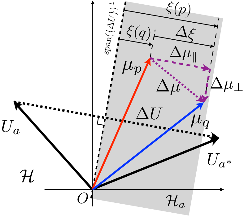
(a) Illustration of EUM in ${\mathcal{H}}$ for PCE ($n_{\Delta\mu_{\parallel}}=n_{\Delta{U}}$).

(b) An example of PIE $\Delta\mu_{\perp}$ and PCE $\Delta\mu_{\parallel}$ when ${\footnotesize\langle{\Delta\mu_{\parallel}},{\Delta{U}}\rangle}>0$ .

Figure 8: Illustration of TIP for the planning-critical error (PCE). In ($a$), $\Delta{U}={U}_{{a}^{*}}-{U}_{{a}}$ defines the behaviour direction; $\xi$ represents the preference score; $\mu_{p}$ and $\mu_{q}$ are the embeddings of the ground truth and perception result, respectively; $\Delta\mu$ is the perception error, which is decomposed into the planning-critical error (PCE) $\Delta\mu_{\parallel}$, and the planning-invariant error (PIE) $\Delta\mu_{\perp}$; and the shaded area corresponds to ${\mathcal{H}}_{a}$. Note that ${\footnotesize\langle{\Delta\mu_{\parallel}},{\Delta{U}}\rangle}>0$ in this case. In ($b$), an AV is moving forward on a road of width $6$m, A cone is in front of the AV, with its position distributed on a line across the road (the $x$ axis). The ground truth distribution ${p}$ is $\mathcal{U}_{[-1.5,1.5]}$, a uniform distribution with support $[-1.5,1.5]$, while the perception believes its location (distributed as ${q}$) is $\mathcal{U}_{[-0.5,0.5]}$. The $2$m-wide AV has two action options: (i) to make a hard brake and come to a full stop before the $x$-axis (${a}^{*}$, the red solid line with an arrowhead), and the utility function is a constant ${U}_{1}(x)=-5$ with $x$ being the position of the cone (loss of hard braking is identical regardless of the cone position); (ii) to move forward (${a}$, the grey dashed line with an arrowhead), and the utility function is ${U}_{2}(x)=-10\cdot\bm{1}{x\in[-1,1]}$ (only large loss for collision with the cone). The $\Delta{U}$ and $\Delta\mu$ are illustrated in the top right, while the decomposition of PIE $\Delta\mu_{\perp}$ and PCE $\Delta\mu_{\parallel}$ are in the bottom right. Note that, $\Delta\mu_{\parallel}$ is of the same shape as $\Delta{U}$ (thus ${\footnotesize\langle{\Delta\mu_{\parallel}},{\Delta{U}}\rangle}>0$), and $\left\langle\Delta{U},\Delta\mu_{\perp}\right\rangle=0$.

Appendix B Scenario Collection

The scenarios used in this work are curated from AV road tests in real world from public roads in urban areas of megacities, e.g. central business districts, populated residential communities, major commercial areas, etc. Each scenario is a 10s-long excerpt extracted from a continuous interval of a road test, which consists of (i) all raw data recordings (LiDAR point clouds, camera images, positioning signals, etc.) from the road test within the interval, and (ii) the portion of offline generated high-definition (HD) and birds-eye view (BEV) raster maps that cover the field of perception during the interval. The duration of a road test ranges from tens of minutes to several hours, and covers various times on both weekdays and weekends from early morning till late night during a period of more than one year, providing a rich blending in weather condition (e.g. sunny, cloudy, rainy, and snowy), traffic intensity (e.g. congested highways during rush hours and crowded streets on holidays), road participant diversity (e.g. private cars, cyclists, pedestrians, and emergency vehicles), and so forth. The scenarios are selected from non-trivial situations (i.e. those with few traffic participants are filtered out) with a balance in AV motion speed, diversity of traffic participants, weather, geographical locations, etc.

Appendix C Autonomous Vehicle Planner

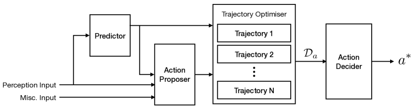
Figure 9: Diagram of the major components in the planner used in the experiment.

Table 3: Comparison of perception metrics for autonomous driving.

Metric	NDS (Caesar et al., 2020)	SDE-APD (Deng et al., 2021)	PKL (Philion et al., 2020)	IPA (Ivanovic & Pavone, 2022)	TIP
Metric Parametri- sation	Manual	Manual + calibration	None	None	None
Evaluable Error Types	Detection, category, velocity, heading, localisation, size	Vehicle size, heading, location	Any perception inputs to the planner	Any perception inputs to the planner in the differentiable cost terms	Any perception inputs to the planner
Perception Input Represen- tation	Deterministic	Deterministic	Deterministic	Deterministic	Either deterministic or probabilistic
Reflecting Actual Severity?	Not necessary	Not necessary	Partially	For small local errors in the differentiable terms only	Yes
Planner Dependence	None	None	Planners with probabilistic trajectory output	Planners with differentiable cost functions	Planners with action-state utility functions
Planner Specifi- cation	None	None	Training data, planner network, learning algorithm (for neural planners)	Cost function weights	Utility function parameters and weights
Planner for Empirical Study	None	None	End-to-end planning architectures trained on nuScenes training set	Learnt from human driving records in nuScenes	Tuned/learnt from real world road test scenarios and human driving records
Planner Validation	None	None	Validated on 4k nuScenes trajectories (<200 miles in total length)	Validated on 4k nuScenes trajectories (<200 miles in total length)	Validated on 100k miles real world urban road test (>100 MPI)

Our planner is designed to control SAE Level 4 AVs operating in urban areas of major modern cities. Its modularised architecture consists of four major components as illustrated in Figure 9:

• The predictor infers the motion information ${s}_{m}$ in the future (i.e. $t>0$) for all dynamic road objects from perception input history (i.e. $t\leqslant 0$) up to the planning time (i.e. $t=0$).

• The action proposer analyses the current environment at the planning time from (i) the perception input, (ii) future object motion input, and (iii) other input signals (e.g. localisation, traffic lights, semantic maps, routing path, etc.), and proposes various sets of behaviours (e.g. ‘go straight’ and ‘lane change’) for the AV with an initial feasible spatiotemporal trajectory for each set.

• The trajectory optimiser takes the results of the above components as input and finds the optimal spatiotemporal trajectory for each behaviour set by numerically solving an optimisation problem with the initial feasible trajectory from the proposer as the starting point.

• The optimal trajectories from all behaviour sets are then submitted to the action decider, which assembles all information to evaluate the utilities of different candidate actions (with corresponding optimal spatiotemporal trajectories), and makes the final decision on ${a}^{*}$.

The utility function ${U}({a},{s})$ of the planner is of the general form

$${U}({s},{a})=\sum\nolimits_{i}\prod\nolimits_{j=1}^{n_{j}}\lambda_{ij}{U}_{ij}({s},{a})+{U}_{s}({s})+{U}_{a}({a}),$$

where $\{\lambda\}$ are the (static) coefficients, the atomic element function ${U}_{i}$ depending on both ${a}$ and ${s}$ characterises the “compatibility” of action ${a}$ and scenario ${s}$, ${U}_{s}({s})$ depicts the current environment, and ${U}_{a}({a})$ evaluates the quality of the action. These terms can be categorised into the following groups.

• The smooth motion group encourages motion without abrupt change in acceleration and penalises large jerks (i.e. the derivative of acceleration).

• The safety distance to obstacles group is designed to keep the AV away from other road objects to minimise the collision likelihoods and guarantee leeway for control. This distance is defined as the $\ell^{2}$ distance between the AV spatiotemporal sweeping contour and a foreign object on the road.

• The legal motion satisfaction group is designed to enforce the AV to strictly follow all applicable traffic rules when in motion. For instance, the cost of crossing solid yellow lines is made significant such that the behaviour is prohibited unless a collision cannot be avoided otherwise. Some other legal options also come at certain costs to discourage high-risk behaviours (e.g. lane changes in crowded scenes).

• The progress to the destination group aims to guide the AV to achieve goals in distant horizons and reach the final destination.

The aforementioned planner deployed onboard our AVs has gone through rigorous road tests in urban areas of major cities with millions of population. Results from 10,000-mile weekly road tests indicate that the planner achieves 111.3 miles per intervention (MPI), confirming that the planner used in this work is a reasonable and validated one.

Appendix D More Comparisons to Related Metrics

In comparison to the other baseline metrics, e.g. PKL (Philion et al., 2020) and IPA (Ivanovic & Pavone, 2022) that are recently proposed for evaluating perception in the context of autonomous driving, our approach provides a universal and principled solution to evaluate the impact of perception noises from the perspective of the planning process of an AV. Highlights of comparison across these two and other perception metrics for autonomous driving are summarised in Table 3.

D.1 Comparison with PKL

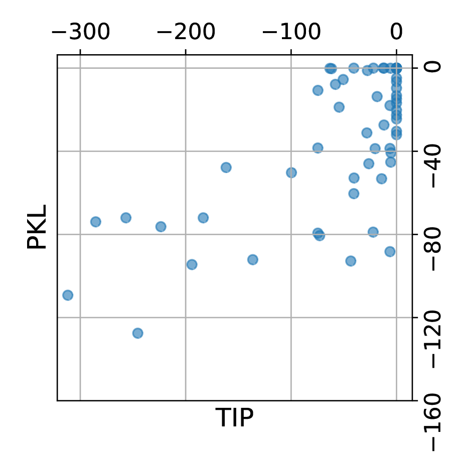
(a) Scatter plot of PKL and TIP scores.

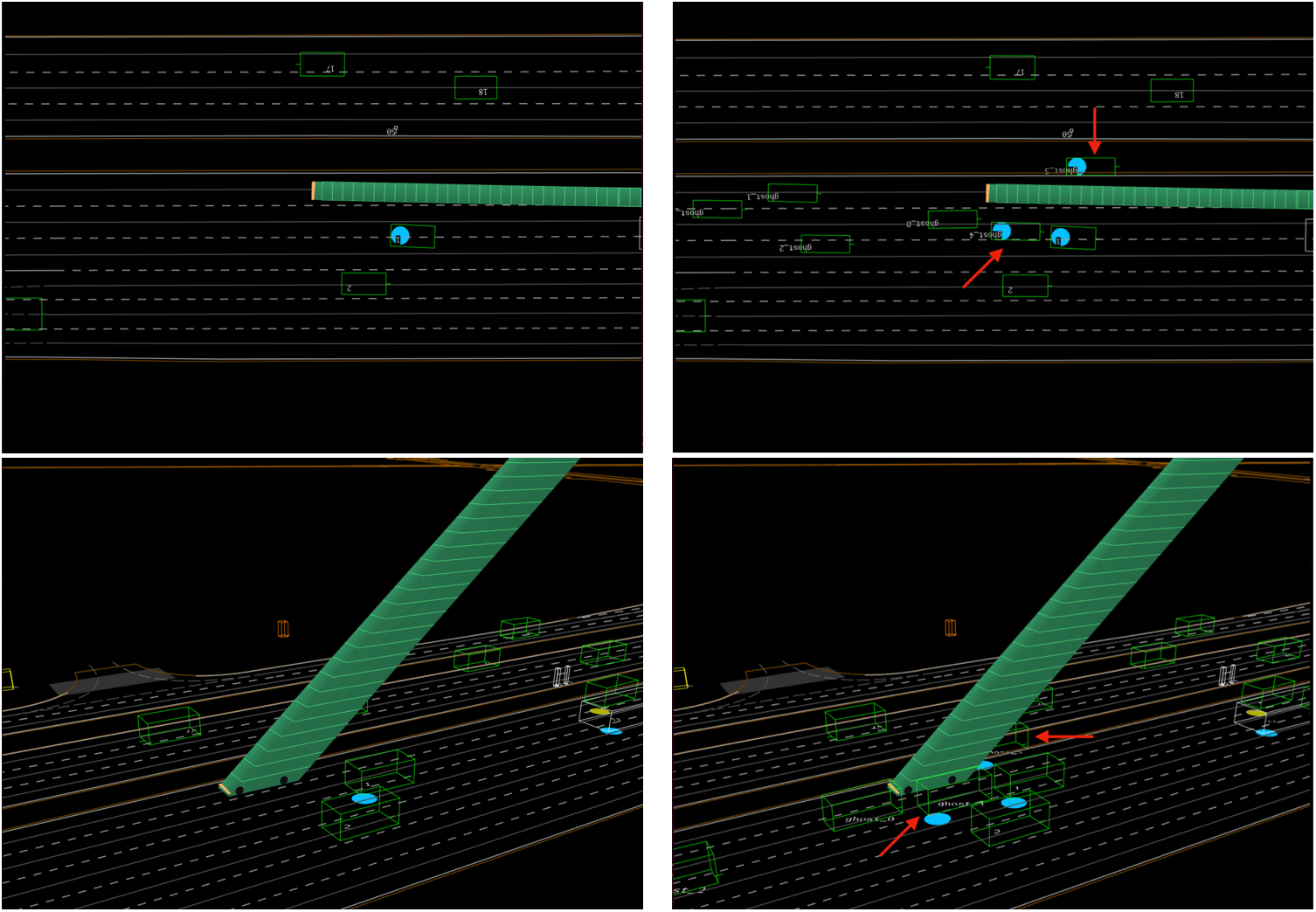
(b) Illustration of AV behaviours in the ground truth and synthetic scenes with false positives.

Figure 10: Result on the false positive synthetic data (best viewed in colour). In ($a$), the data points (downsampled for clarity) close to $x$-axis (PKL = 0) correspond to the cases where the AV behaviours under the ground truth and noisy perception inputs are identical. The data points close to $y$-axis (TIP = 0) correspond to the cases where the AV planning preference between the optimal action and others is identical under ground truth and noisy perception inputs. Note the number of cases where TIP disagrees with PKL on the impact on AV planning. In ($b$), The green tube represents the spatiotemporal trajectory of the AV with the z-axis as the temporal dimension (same for the rest). Bold solid lines are the boundary of driving areas (e.g. curbs, vegetarian zoom dividers), while light solid lines are the centre lines of vehicle lanes with dashed lines as the lane boundaries. Road objects are marked with 3D bounding boxes in green. Sub-figures in the first (second) row are birds-eye view (side view) of the scene and sub-figures in the left (right) column correspond to ground truth (noisy) perception input (same for the rest). In this case, the AV intends to move forward under the ground truth perception input (left column); in the presence of perception input noise (right column), the AV behaviour remains almost unchanged (PKL = -0.248), since two false positive vehicles (pointed by red arrows) on both sides force the AV to keep moving straight, yet the close-to-object cost (safety distance to road obstacles) has changed considerably during planning, leading to a TIP score of -61.654.

More empirical results are provided to better understand the difference between the proposed TIP and PKL (Philion et al., 2020).

Results on Synthetic Data. Figure 10(a) demonstrates a scatter plot for scene-wise TIP and PKL results on the synthetic data generated as described in Section 5.2 with 6 false positives per scene. It is observed that some results are very close to either $x$- or $y$-axis, suggesting that TIP and PKL deviate in deciding if a perception error (i.e. false positive) is crucial to planning in these cases. A typical scenario of such disagreement is shown in Figure 10(b), where the behaviour of the AV does not change significantly with ground-truth or noisy perception inputs (PKL = -0.248), yet the planning process has changed quite a lot (TIP = -61.654) due to the affinity of false positive objects that have drastically change the planning cost to close objects. In this case, TIP is capable of detecting serious perception errors that PKL fails to identify.

Results on Real Data. On the real data, we also have similar observations, which is demonstrated by an actual scene for one such scenario in Figure 11: a falsely detected vehicle in front of the AV does not change the AV’s behaviour considerably (PKL = -0.802), while the significant planning cost change is reflected by TIP with a value -115.42. More individual examples are shown in Figure 12.

Overall, on both synthetic and real data, the proposed TIP is shown to efficiently and effectively capture perception errors critical to AV planning that may be missed by PKL. This confirms our motivation to exploit the actual AV planning process, as opposed to the planning result only, to gain insights into the impact of input perception error on AV driving quality.

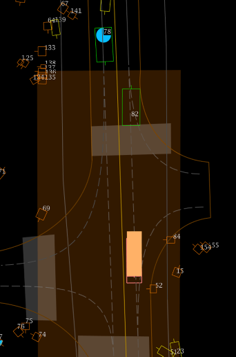
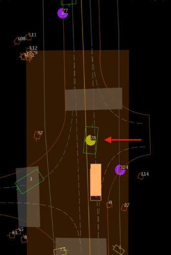
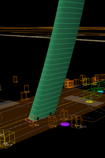
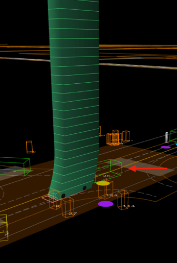
Figure 11: Illustration of AV behaviours in reaction to ground truth and actual noisy perception inputs (best viewed in colour). Under the ground truth perception input (the first and the third pictures), the AV is clear to move forward with soft braking to keep distance to another vehicle (‘82’) in front. Given the noisy perception input (the second and the fourth pictures), however, the AV has to hard brake to avoid a potential collision with the false positive vehicle (‘28’) close to it in front (marked by the red arrow). In both cases, since the AV speed is slow and is braking (either soft or hard), the difference in behaviour is insignificant (PKL = -0.802), yet the consequence of the false positive is by no means trivial: the false positive causes a hard brake and virtual collision (between the behaviours given ground truth perception input and false positive), which is precisely captured by the proposed TIP (-115.42). The kinematic motion for the ground truth scenario (bottom left) is $a=-0.36$m/s², $j=-0.72$m/s³, and for the noisy scenario (bottom right) is $a=-0.36$m/s², $j=-76.4$m/s³. Note how sharp the braking changes in presence of the noisy perception (jerk: $-0.72$m/s³ versus $-76.4$m/s³). Clearly, this is a critical error from the system’s perspective.

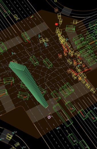
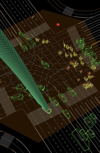
Figure 12: Illustration of more AV behaviours in reaction to ground truth and actual noisy perception inputs (best viewed in colour). Two more outrageous perception errors are shown where an object location is improperly perceived such that it is superimposed with the AV. The ground truth is shown in the first and third pictures and the actual noisy perception in the second and fourth, respectively. For the first case: TIP = -132.4, PKL = 0.0. For the second case: TIP = -75.0, PKL = 0.04.

D.2 Comparison with IPA

Injecting planning-awareness (IPA) is recently proposed by (Ivanovic & Pavone, 2022) to encode the planning error based on the hypothesis that the impact of an object location error is proportional to the gradient magnitude of the planning cost functions involving the AV-object distance. This solution requires differentiability of the planning cost functions, while our approach does not and thus is more applicable to a modularised SAE Level 4 AV that typically comprises a pipeline of individual components including perception (Luo et al., 2021b), prediction (Wang et al., 2023), planning (Bronstein et al., 2022), etc. Even more serious, IPA fails to account for all cases since the local properties (gradients) do not always reflect the global ones (overall losses). To illustrate this, consider a scenario, where the cost of AV being close to an object is $1/d$. Now assume that there are two cases of object location errors.

• Case one: The ground truth distance of an object to the AV is 1m, and the noisy distance estimated by perception is 0.9m. Per IPA defined in (Ivanovic & Pavone, 2022), the result is

  $$\mathinner{\!\left\lvert\left.\frac{\operatorname{d\!}}{\operatorname{d\!}d}(1/d)\right|_{d=1}\right\rvert}\mathinner{\!\left\lvert\Delta d\right\rvert}=1\times\mathinner{\!\left\lvert 1.0-0.9\right\rvert}=0.1,$$

  while the actual cost difference is $\mathinner{\!\left\lvert\frac{1}{0.9}-\frac{1}{1}\right\rvert}=1/0.9-1=0.111$.

• Case two: The ground truth distance of an object to the AV is 2m, and the noisy distance estimated by perception is 2.5m. Per IPA defined in (Ivanovic & Pavone, 2022), the result is

  $$\mathinner{\!\left\lvert\left.\frac{\operatorname{d\!}}{\operatorname{d\!}d}(1/d)\right|_{d=2}\right\rvert}\mathinner{\!\left\lvert\Delta d\right\rvert}=0.25\times\mathinner{\!\left\lvert 2.5-2.0\right\rvert}=0.125,$$

  while the actual cost difference is $\mathinner{\!\left\lvert\frac{1}{2}-\frac{1}{2.5}\right\rvert}=0.5-1/2.5=0.1$.

Obviously, IPA score of case two is larger than case one, while the actual error in planning cost is the other way, as the Taylor series up to first-order terms adopted by IPA cannot precisely delineate the cost function value change over a large input variation.

Appendix E Application to Neural Planners

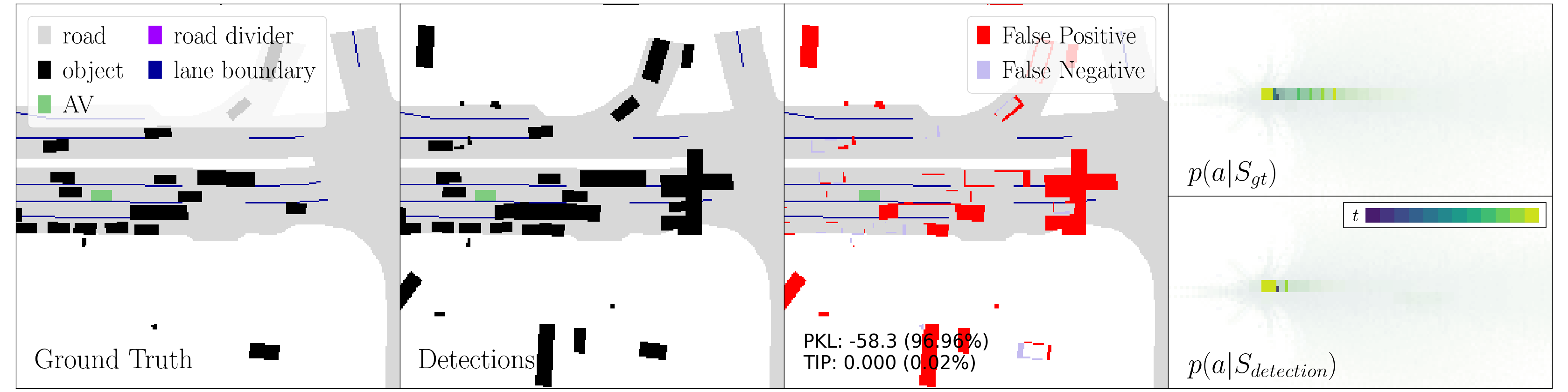
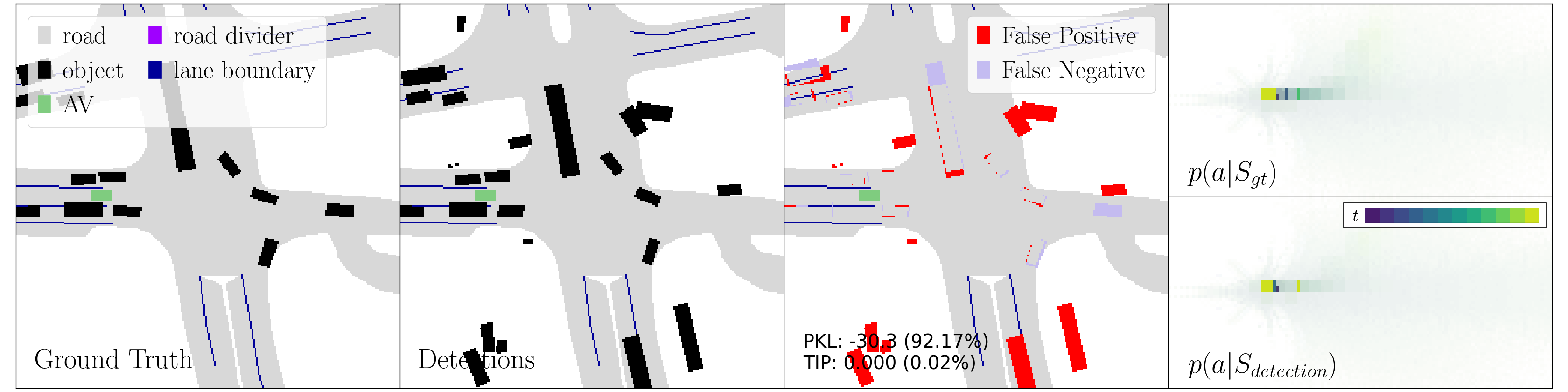
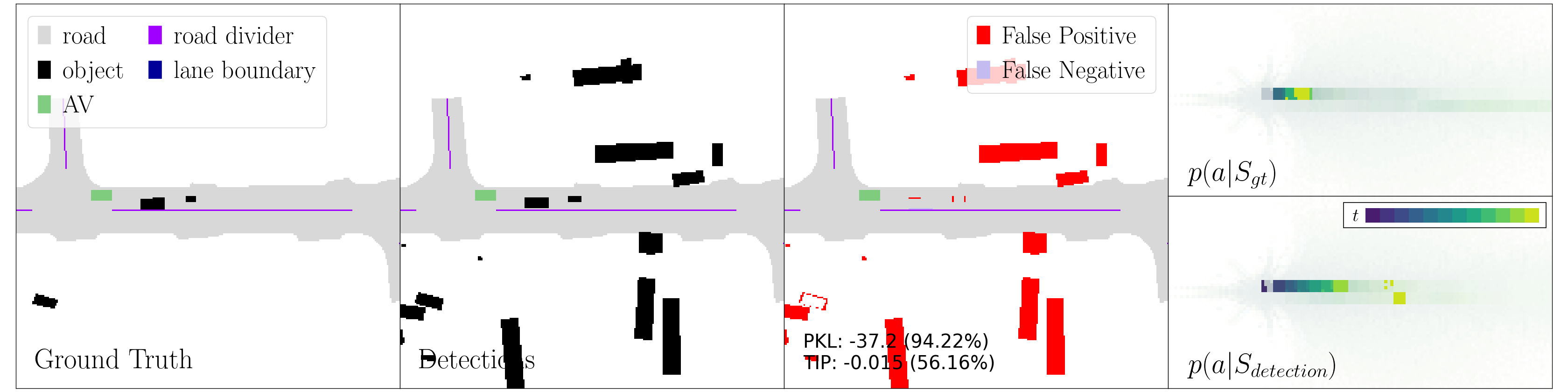
Figure 13: Detection results and metric scores on nuScenes dataset (best viewed in colour). From left to right columns: (i) ground truth annotations; (ii) detection results; (iii) difference between ground truth and detection results, with PKL and TIP scores for the scenario (score percentiles in the whole dataset are also shown in parentheses); and (iv) AV location distributions ${p}({a}|S)={p}(\{l_{t}\}|S)$ at different time steps predicted by the planner, with one colour map corresponding to the location distribution at one time step (the action distribution density has been enhanced for visual saliency and not plotted to the numeric scale, and the most likely positions at each time step are marked with the corresponding solid colour).

Following the discussion in Section 5.4, more scenarios where PKL and TIP scores differ are illustrated in Figure 13 for detection results by the CBGS detector on nuScenes validation dataset. A typical observation is that, for the neural planner employed, when the optimal AV action (subject to kinetic and kinematic constraints) is to remain stationary regardless of the input perception noises (the first two examples in Figure 13), TIP generally predicts an insignificant impact of the error while PKL may be dominated by the difference in low-probability regions where the KL-divergence is considerable (note that the result $p\log\frac{p}{q}$ could be large for any given $p>0$ when $q\rightarrow 0$). For similar reasons, PKL also tends to overestimate the impact in some cases where the AV is not stationary (the third example in Figure 13).

In addition to scoring a particular detection result, the proposed metric can also predict sensitive regions where false positives or true positives are most crucial for a planner. For this, we measure the impact of false negatives by removing vehicles from the ground truth annotations and evaluating the TIP score of the synthetic scene, with results presented in Figure 14. Similarly, the significance of false positives is predicted by adding a ghost vehicle at a location and evaluating the TIP score of the scene, which is illustrated in Figure 15. Overall, the most critical false positives or negatives are identified at the locations along the future spatiotemporal path of the AV that require AV-object interaction. Interestingly, the neural planner may reverse in some cases, producing nontrivial TIP scores for false positives or negatives behind it. This observation is distinct from that in Section 5.2.2, where a false negative behind the AV has no impact on the AV planner that does not reverse.

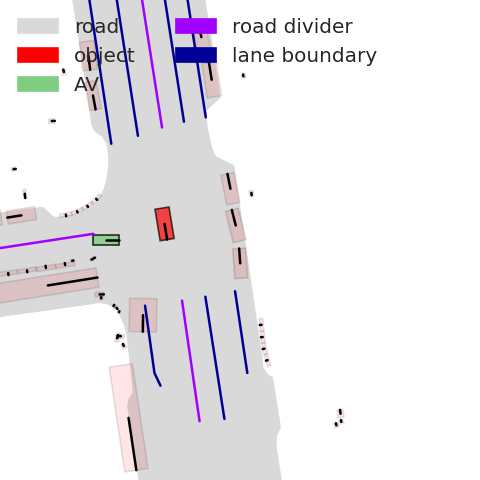
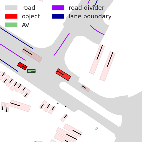
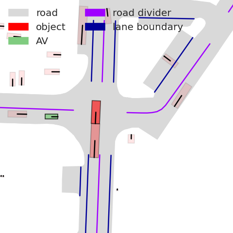
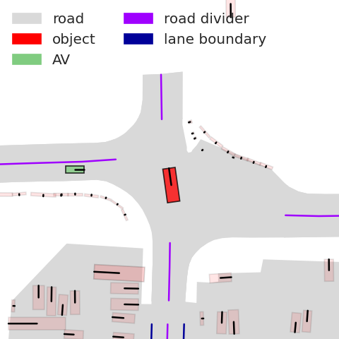
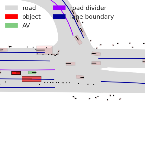
Figure 14: Examples of crucial false negatives predicted by TIP (best viewed in colour). The colour saturation indicates the significance of the error if the corresponding vehicle is missed by the detector.

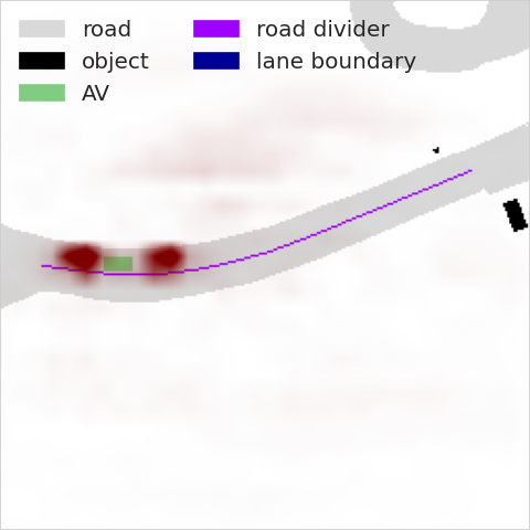
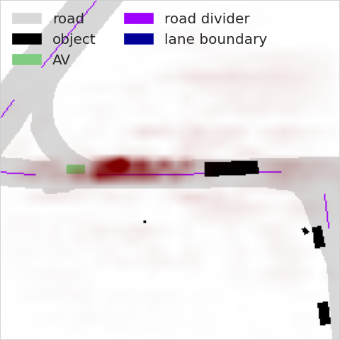
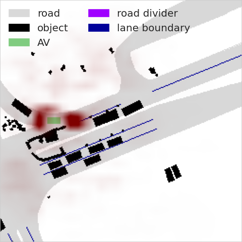
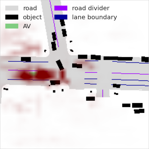
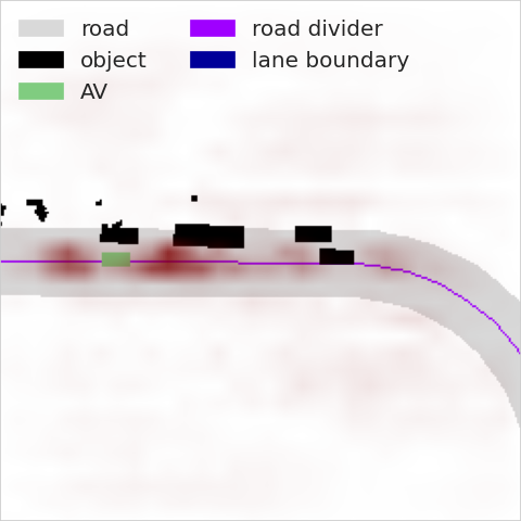
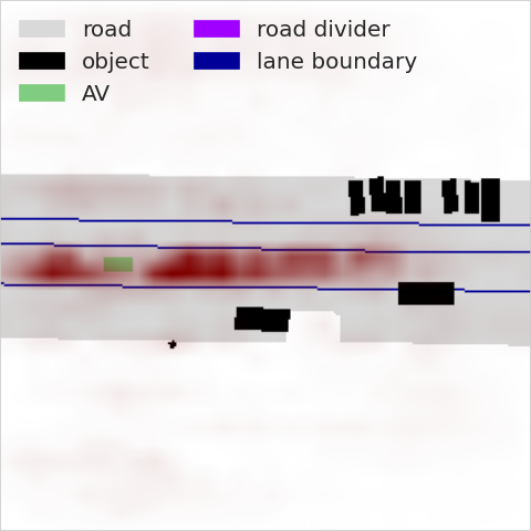
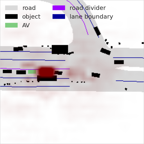
Figure 15: Examples of crucial false positives predicted by TIP (best viewed in colour). The colour saturation indicates the significance of the error if a ghost vehicle is falsely detected at the corresponding location.

Appendix F Examples and Non-Examples of Square-Integrable Density Functions

Theorem 3.1 in the main text requires square-integrability of a density function, which includes many popular cases that may be used for constructing the utility function for planning.

Example 1 (Bounded PDFs).

If both the support and range of the PDF $f(x)$ of a random variable are bounded, then $f(x)$ is square-integrable, e.g. uniform distribution.  

Example 2 (Parametric PDFs).

PDFs of many popular parametric statistical models are square-integrable, e.g.  (sub-)Gaussian, (sub-)Laplace, Gamma (including exponential, Erlang, and $\chi^{2}$ distribution), etc.  

Example 3 (Mixture Models of Countable Components with Square-Integrable PDFs).

The PDF of a mixture model is of the form:

$$f(x)=\sum\nolimits_{i}\alpha_{i}f_{i}(x),~{}\alpha_{i}>0,~{}\sum\nolimits_{i}\alpha_{i}=1,$$ (13)

where $f_{i}(x)$ is the PDF of the $i$-th component out of the countable set $\{f_{i}(x)\}$. $f(x)$ of (13) is square-integrable if $\forall i,f_{i}\in L^{2}$ and $M=\sup_{i}\mathinner{\!\left\lVert f_{i}\right\rVert}_{\mathcal{H}}<+\infty$ as

$$\int\mathinner{\!\left\lvert f(x)\right\rvert}^{2}\operatorname{d\!}x =\int\sum_{i,j}\alpha_{i}\alpha_{j}f_{i}(x)f_{j}(x)\operatorname{d\!}x=\sum_{i,j}\alpha_{i}\alpha_{j}\left\langle f_{i},f_{j}\right\rangle_{\mathcal{H}}$$ (14)

$$\leqslant\sum_{i,j}\alpha_{i}\alpha_{j}\mathinner{\!\left\lVert f_{i}\right\rVert}_{\mathcal{H}}\mathinner{\!\left\lVert f_{j}\right\rVert}_{\mathcal{H}}\leqslant M^{2}<+\infty.$$

A variety of mixture models are included such as Gaussian mixture models and mixtures of Gamma distribution.  

On the other hand, since $\ell^{1}$ and $\ell^{2}$ norms are not necessarily equivalent in infinite-dimensional spaces, there are indeed some density functions $f(x)\in L^{1}$ with infinite $\ell^{2}$ norm.

Non-Example 1 (Square-Unintegrable PDFs).

Let the distribution ${F}_{X}$ of a random variable $X$ be

$${F}_{X}(x)=\begin{cases}0,&x\in(-\infty,0)\\ \frac{1}{\sqrt{a}}x^{\frac{1}{2}},&x\in[0,a]\\ 1,&x\in(a,+\infty)\end{cases}$$

where $a>0$ is the parameter; and the density function is then

$$f(x)=\begin{cases}\frac{1}{2\sqrt{a}}x^{-\frac{1}{2}},&x\in(0,a)\\ 0,&\textnormal{otherwise}\end{cases}$$

where $f(x)$ is not square-integrable since $x^{-1}$ increases too fast as $x\rightarrow 0$.  

Appendix G Proofs of Theorems in the Main Text

G.1 Notations

Besides the notations in Section 3.1, a few more are introduced as follows. A unit step function is $W(x-c)=\bm{1}{x\in[c,+\infty)},c\in\mathbb{R}$. $L^{1}({\mathcal{X}},\rho)$ denotes the space of absolutely integrable functions.

G.2 Embedding Probability Measures in ${\mathcal{H}}$

Proof (Theorem 3.1).

Since ${F}_{X}(x)$ is absolutely continuous, there exists a density function $f_{X}(x)\in L^{1}$ such that

$$\frac{\operatorname{d\!}}{\operatorname{d\!}x}{F}_{X}(x)=f_{X}(x)$$ (15)

almost everywhere. Since $f_{X}(x)\in L^{2}$ , let $M=\mathinner{\!\left\lVert f_{X}\right\rVert}<+\infty$, $\forall g\in{\mathcal{H}}$, we have

$$\mathinner{\!\left\lvert\mathbb{E}_{X}\left[g(x)\right]\right\rvert}= ~{}\mathinner{\!\left\lvert\int_{x}g(x)\operatorname{d\!}F_{X}(x)\right\rvert}$$ (16)

$$= ~{}\mathinner{\!\left\lvert\int_{x}g(x)f(x)\rho(\operatorname{d\!}x)\right\rvert}$$ (17)

$$\leqslant ~{}\int_{x}\mathinner{\!\left\lvert g(x)\right\rvert}\mathinner{\!\left\lvert f(x)\right\rvert}\rho(\operatorname{d\!}x)$$ (18)

$$\leqslant ~{}M||g||_{{\mathcal{H}}},$$ (19)

where (19) follows from the Cauchy-Schwarz inequality (Rudin, 1976, Theorem 11.35). Thus, the linear functional $\mathbb{E}_{X}\left[\cdot\right]$ is bounded on ${\mathcal{H}}$ and

$$\mathbb{E}_{X}\left[g(x)\right]=\int_{x}g(x)\operatorname{d\!}{F}_{X}(x)=\int_{x}f_{X}(x)g(x)\rho(\operatorname{d\!}x)=\left\langle f_{X},g\right\rangle_{\mathcal{H}},~{}\forall g\in{\mathcal{H}},$$

where $\mu_{p}\coloneqq f_{X}\in{\mathcal{H}}$ is the embedding of the probability measure in ${\mathcal{H}}$. Now assume that there exists another element $\mu^{\prime}\in{\mathcal{H}}$ such that

$$\mathbb{E}_{X}\left[g(x)\right]=\left\langle\mu^{\prime},g\right\rangle_{\mathcal{H}},~{}\forall g\in{\mathcal{H}}.$$

Since $\mu_{p}-\mu^{\prime}\in{\mathcal{H}}$, we have

$$\mathinner{\!\left\lVert\mu_{p}-\mu^{\prime}\right\rVert}^{2}_{\mathcal{H}}= ~{}\left\langle\mu_{p}-\mu^{\prime},\mu_{p}-\mu^{\prime}\right\rangle_{\mathcal{H}}$$

$$= ~{}\left\langle\mu_{p},\mu_{p}-\mu^{\prime}\right\rangle_{\mathcal{H}}-\left\langle\mu^{\prime},\mu_{p}-\mu^{\prime}\right\rangle_{\mathcal{H}}$$

$$= ~{}\mathbb{E}_{X}\left[\mu_{p}-\mu^{\prime}\right]-\mathbb{E}_{X}\left[\mu_{p}-\mu^{\prime}\right]$$

$$= ~{}0.$$

Therefore, the embedding $\mu_{p}$ for probability measure ${p}$ in ${\mathcal{H}}$ is a unique equivalence class of the functions that are equal almost everywhere.  

G.3 Injection of Probability Measure Embeddings in ${\mathcal{H}}$

To prove the injection of probability measure embedding in Theorem 3.2, a preliminary result is first introduced.

Lemma G.1 (Lemma 9.3.2 of (Dudley, 2002)).

If $({\mathcal{X}},{\mathtt{d}})$ is a metric space, ${p}$ and ${q}$ are two probability measures on ${\mathcal{X}}$, then $\mathbb{E}_{x\sim{p}(x)}\left[g\right]=\mathbb{E}_{x\sim{q}(x)}\left[g\right],\forall g\in C_{b}({\mathcal{X}})$ if and only if ${p}={q}$, where $C_{b}({\mathcal{X}})$ is the space of all bounded continuous functions on ${\mathcal{X}}$.

Proof (Theorem 3.2).

Now we prove this theorem in the following two directions.

Necessity. Since the embedding of a probability measure is unique in ${\mathcal{H}}$, it is easy to see that $\mu_{p}=\mu_{q}$ if ${p}={q}$.

Sufficiency. Note that, by Weierstrass extreme value theorem (Rudin, 1976, Theorem 4.16), any real continuous function $g\in C({\mathcal{X}})$ on the compact space ${\mathcal{X}}$ is bounded, i.e.$\forall g\in C({\mathcal{X}}),\exists M\in\mathbb{R}$ such that $\mathinner{\!\left\lvert g(x)\right\rvert}<M,\forall x\in{\mathcal{X}}$. It follows that $C({\mathcal{X}})\subset L^{2}({\mathcal{X}})$ since

$$\int_{\mathcal{X}}\mathinner{\!\left\lvert g(x)\right\rvert}^{2}\rho(\operatorname{d\!}x)\leqslant M^{2}\mathinner{\!\left\lvert{\mathcal{X}}\right\rvert}<+\infty.$$

Now if $\mu_{p}=\mu_{q}$ almost everywhere, we have

$$\mathinner{\!\left\lvert\mathbb{E}_{{p}}\left[g(x)\right]-\mathbb{E}_{{q}}\left[g(x)\right]\right\rvert} =\mathinner{\!\left\lvert\left\langle\mu_{p},g\right\rangle-\left\langle\mu_{q},g\right\rangle\right\rvert}=\mathinner{\!\left\lvert\left\langle\mu_{p}-\mu_{q},g\right\rangle\right\rvert}$$ (20)

$$\leqslant\mathinner{\!\left\lVert\mu_{p}-\mu_{q}\right\rVert}_{\mathcal{H}}\mathinner{\!\left\lVert g\right\rVert}_{\mathcal{H}}=0,~{}\forall g\in C({\mathcal{X}}).$$ (21)

Thus ${p}={q}$ by Lemma G.1.  

G.4 Approximation of Expectation for Discrete/Mixed distribution in ${\mathcal{H}}$

While Theorem 1 in the main text only addresses the continuous distribution, a similar result can be found given point-wise continuity conditions for general distribution, which can be decomposed into absolutely continuous and discrete parts (Chung, 2000).

Theorem G.4 (Approximation of Mixed Distribution).

Let ${F}_{ac}(x)$ be an absolutely continuous distribution function with density function $f_{X}(x)$; ${F}_{d}(x)=\sum_{i}b_{i}W(x-a_{i})$ a discrete distribution function of point mass at a countable set $\{a_{i}\}$ such that $b_{i}>0$ and $\sum_{i}b_{i}=1$; ${F}_{X}(x)=\lambda{F}_{ac}(x)+(1-\lambda){F}_{d}(x)$ a mixed distribution function with $\lambda\in(0,1)$ as the convex combination coefficient. If $f_{X}(x)$ is square-integrable, and $g(x)\in L^{2}$ is uniformly continuous at $\{a_{i}\}$, then there exists a sequence of $\{\mu_{{p},n}\}\subset{\mathcal{H}}$ such that

$$\lim_{n\rightarrow\infty}\left\langle{\mu_{{p},n}},g\right\rangle_{{\mathcal{H}}}=\mathbb{E}_{X}\left[g(x)\right].$$ (22)

We start by considering a simple discrete case by the following lemma.

Lemma G.5.

Let ${F}_{X}(x)=W(x-a)$ be a discrete distribution function with point mass at $a\in{\mathcal{X}}$. If $g(x)\in L^{2}$ is continuous at $a$, then there exists a sequence of $\{\mu_{{p},n}\}\subset{\mathcal{H}}$ such that

$$\lim_{n\rightarrow\infty}\left\langle{\mu_{{p},n}},g\right\rangle_{{\mathcal{H}}}=\mathbb{E}_{X}\left[g(x)\right].$$ (23)

Proof (Lemma G.5).

$\forall\varepsilon>0$, since $g(x)$ is continuous at $a$, there exists a a radius $r>0$ such that

$$g(a)-\varepsilon\leqslant g(x)\leqslant g(a)+\varepsilon,~{}\forall x\in B(a,r)$$

with a positive measure $V=\rho(B(a,r))>0$, where $B(a,r)\subset{\mathcal{X}}$ is a neighbourhood of $r$ around $a$. Define

$$h_{\varepsilon}(x)=\frac{1}{V}\bm{1}{x\in B(a,r)}\in{\mathcal{H}}.$$

We have

$$g(a)-\varepsilon<\left\langle h_{\varepsilon},g\right\rangle_{{\mathcal{H}}}<g(a)+\varepsilon.$$

Thus,

$$\lim_{n\rightarrow\infty}\left\langle{h_{\frac{1}{n}}},g\right\rangle_{{\mathcal{H}}}=g(a)=\mathbb{E}_{X}\left[g(x)\right].$$

 

Lemma G.5 implies that the expected value of a function continuous at the point mass of a delta distribution can be approximated by an inner product in ${\mathcal{H}}$ with any arbitrary precision.

Proof (Theorem G.4).

Note that

$$\mathbb{E}_{X}\left[g(x)\right]=\lambda\int_{x}g(x)\operatorname{d\!}{F}_{ac}(x)+(1-\lambda)\sum\nolimits_{i}b_{i}g(a_{i}).$$

Since ${F}_{ac}(x)$ is absolutely continuous, by Theorem 1, there exists a $\mu\in{\mathcal{H}}$ such that

$$\int_{x}g(x)\operatorname{d\!}{F}_{ac}(x)=\left\langle\mu,g\right\rangle_{\mathcal{H}},~{}\forall h\in{\mathcal{H}}.$$ (24)

On the other hand, $\forall\varepsilon>0$, since $g(x)$ is uniformly continuous at $\{a_{i}\}$, there exists a radius $r>0$ such that $\forall i$,

$$g(a_{i})-\varepsilon<g(x)<g(a_{i})+\varepsilon,~{}\forall x\in B(a_{i},r)$$

and $V=\rho(B(a_{i},r))>0$ (translation invariance of Lebesgue measures in $\mathbb{R}^{d}$). Define

$$h_{\varepsilon}(x)=\frac{1}{V}\sum\nolimits_{i}b_{i}\bm{1}{x\in B(a_{i},r)}\in{\mathcal{H}}.$$

We have

$$\sum\nolimits_{i}b_{i}g(a_{i})-\varepsilon=\sum\nolimits_{i}b_{i}g(a_{i})-\varepsilon\sum\nolimits_{i}b_{i}<\left\langle h_{\varepsilon},g\right\rangle_{{\mathcal{H}}}<g(a)+\varepsilon\sum\nolimits_{i}b_{i}=\sum\nolimits_{i}b_{i}g(a_{i})+\varepsilon,$$

Thus

$$\lim_{n\rightarrow\infty}\left\langle{h_{\frac{1}{n}}},g\right\rangle_{{\mathcal{H}}}=\sum\nolimits_{i}b_{i}g(a_{i}).$$ (25)

Combining (24) and (25) leads to

$$\lim_{n\rightarrow\infty}\left\langle{\lambda\mu+(1-\lambda)h_{\frac{1}{n}}},g\right\rangle_{{\mathcal{H}}}=\lambda\int_{x}g(x)\operatorname{d\!}{F}_{ac}(x)+(1-\lambda)\sum\nolimits_{i}b_{i}g(a_{i})=\mathbb{E}_{X}\left[g(x)\right].$$

 

G.5 Uniform Convergence Rate of Expected Utility Estimators

Proof (Theorem 4.1).

Assume that $\{X_{i}\}_{i=1}^{n}$ and independent and $X_{i}\in[a_{i},b_{i}]$ almost surely. Let $\bar{X}=\frac{1}{n}\sum_{i}X_{i}$.

Per Hoeffding’s inequality (Hoeffding, 1963, Theorem 2), for any $\varepsilon>0$,

$$\textup{Pr}\Big{(}\bar{X}-\mathbb{E}\left[\bar{X}\right]>\varepsilon\Big{)}<\exp{\bigg{\{}-\frac{2n^{2}\varepsilon^{2}}{\sum_{i=1}^{n}(b_{i}-a_{i})^{2}}\bigg{\}}}.$$ (26)

By symmetry, it also holds true that, for any $\varepsilon>0$,

$$\textup{Pr}\Big{(}\bar{X}-\mathbb{E}\left[\bar{X}\right]<-\varepsilon\Big{)}<\exp{\bigg{\{}-\frac{2n^{2}\varepsilon^{2}}{\sum_{i=1}^{n}(b_{i}-a_{i})^{2}}\bigg{\}}}.$$ (27)

Combining one-side inequalities of (26) and (27) leads to

$$\textup{Pr}\Big{(}\mathinner{\!\left\lvert\bar{X}-\mathbb{E}\left[\bar{X}\right]\right\rvert}>\varepsilon\Big{)}<2\exp{\bigg{\{}-\frac{2n^{2}\varepsilon^{2}}{\sum_{i=1}^{n}(b_{i}-a_{i})^{2}}\bigg{\}}}\leqslant 2\exp{\bigg{(}-\frac{n\varepsilon^{2}}{2M^{2}}\bigg{)}},~{}\forall\varepsilon>0,$$ (28)

where $M=\sup(\{\mathinner{\!\left\lvert a_{1}\right\rvert},\cdots,\mathinner{\!\left\lvert a_{n}\right\rvert},\mathinner{\!\left\lvert b_{1}\right\rvert},\cdots,\mathinner{\!\left\lvert b_{n}\right\rvert}\})$.

On the other hand, Bernstein inequality (Bernstein, 1946) also provides an improved revision of Chebyshev’s inequality by incorporating both almost-sure bound and variance bound:

$$\textup{Pr}\bigg{(}\mathinner{\!\left\lvert\bar{X}-\mathbb{E}\left[\bar{X}\right]\right\rvert}>\varepsilon\bigg{)}<2\exp\bigg{\{}-\frac{n\varepsilon^{2}}{2\textup{Var}(\bar{X})+2M\varepsilon/3}\bigg{\}},~{}\forall\varepsilon>0.$$ (29)

The proof is completed by setting $X_{i}={U}(S_{i},{a})$ and taking the lowest bound of (28) and (29) for the tail probability of $\mathinner{\!\left\lvert\bar{X}-\mathbb{E}\left[\bar{X}\right]\right\rvert}$.

References

- Ajanovic et al. (2018) Ajanovic, Z., Lacevic, B., Shyrokau, B., Stolz, M., and Horn, M. Search-based optimal motion planning for automated driving. In IROS, 2018.
- Åsljung et al. (2017) Åsljung, D., Nilsson, J., and Fredriksson, J. Using extreme value theory for vehicle level safety validation and implications for autonomous vehicles. IEEE Transactions on Intelligent Vehicles, 2017.
- Bansal et al. (2019) Bansal, M., Krizhevsky, A., and Ogale, A. ChauffeurNet: Learning to drive by imitating the best and synthesizing the worst. In RSS, 2019.
- Bernstein (1946) Bernstein, S. N. The Theory of Probabilities. Gastehizdat Publishing House, 1946.
- Bishop (2006) Bishop, C. M. Pattern Recognition and Machine Learning. Springer-Verlag, 2006.
- Bojarski et al. (2016) Bojarski, M., Del Testa, D., Dworakowski, D., Firner, B., Flepp, B., Goyal, P., Jackel, L. D., Monfort, M., Muller, U., Zhang, J., Zhang, X., Zhao, J., and Zieba, K. End to end learning for self-driving cars. arXiv:1604.07316, 2016.
- Bronstein et al. (2022) Bronstein, E., Palatucci, M., Notz, D., White, B., Kuefler, A., Lu, Y., Paul, S., Nikdel, P., Mougin, P., Chen, H., Fu, J., Abrams, A., Shah, P., Racah, E., Frenkel, B., Whiteson, S., and Anguelov, D. Hierarchical model-based imitation learning for planning in autonomous driving. In IROS, 2022.
- Buehler et al. (2009) Buehler, M., Iagnemma, K., and Singh, S. The DARPA Urban Challenge: Autonomous Vehicles in City Traffic. Springer, 2009.
- Caesar et al. (2020) Caesar, H., Bankiti, V., Lang, A., Vora, S., Liong, V. E., Xu, Q., Krishnan, A., Pan, Y., Baldan, G., and Beijbom, O. nuScenes: A multimodal dataset for autonomous driving. In CVPR, 2020.
- Chung (2000) Chung, K. A Course in Probability Theory. Elsevier Science, 2000.
- Codevilla et al. (2019) Codevilla, F., Santana, E., López, A. M., and Gaidon, A. Exploring the limitations of behavior cloning for autonomous driving. In ICCV, 2019.
- Deng et al. (2021) Deng, B., Qi, C. R., Najibi, M., Funkhouser, T., Zhou, Y., and Anguelov, D. Revisiting 3D object detection from an egocentric perspective. In NeurIPS, 2021.
- Dosovitskiy et al. (2017) Dosovitskiy, A., Ros, G., Codevilla, F., Lopez, A., and Koltun, V. CARLA: An open urban driving simulator. In CoRL, 2017.
- Dudley (2002) Dudley, R. M. Real Analysis and Probability. Cambridge University Press, 2002.
- Fan et al. (2018) Fan, H., Zhu, F., Liu, C., Zhang, L., Zhuang, L., Li, D., Zhu, W., Hu, J., Li, H., and Kong, Q. Baidu Apollo EM motion planner. arXiv:1807.08048, 2018.
- Feng et al. (2022) Feng, D., Harakeh, A., Waslander, S. L., and Dietmayer, K. A review and comparative study on probabilistic object detection in autonomous driving. IEEE Transactions on Intelligent Transportation Systems, 2022.
- Goodfellow et al. (2016) Goodfellow, I., Bengio, Y., and Courville, A. Deep Learning. MIT Press, 2016.
- Grigorescu et al. (2020) Grigorescu, S., Trasnea, B., Cocias, T., and Macesanu, G. A survey of deep learning techniques for autonomous driving. Journal of Field Robotics, 2020.
- Guez et al. (2019) Guez, A., Mirza, M., Gregor, K., Kabra, R., Racanière, S., Weber, T., Raposo, D., Santoro, A., Orseau, L., Eccles, T., Wayne, G., Silver, D., and Lillicrap, T. An investigation of model-free planning. In ICML, 2019.
- Haan et al. (2019) Haan, P. d., Jayaraman, D., and Levine, S. Causal confusion in imitation learning. In NeurIPS, 2019.
- Hoeffding (1963) Hoeffding, W. Probability inequalities for sums of bounded random variables. Journal of the American Statistical Association, 1963.
- Ivanovic & Pavone (2022) Ivanovic, B. and Pavone, M. Injecting planning-awareness into prediction and detection evaluation. In IEEE Intelligent Vehicles Symposium, 2022.
- Kant (1781) Kant, I. Critik der reinen Vernunft. Johann Friedrich Hartknoch, 1781.
- Kendall et al. (2019) Kendall, A., Hawke, J., Janz, D., Mazur, P., Reda, D., Allen, J.-M., Lam, V.-D., Bewley, A., and Shah, A. Learning to drive in a day. In ICRA, 2019.
- Kuefler et al. (2017) Kuefler, A., Morton, J., Wheeler, T., and Kochenderfer, M. Imitating driver behavior with generative adversarial networks. In IEEE Intelligent Vehicles Symposium, 2017.
- Lang et al. (2019) Lang, A., Vora, S., Caesar, H., Zhou, L., Yang, J., and Beijbom, O. PointPillars: Fast encoders for object detection from point clouds. In CVPR, 2019.
- Li et al. (2023) Li, J., Luo, C., and Yang, X. PillarNeXt: Rethinking network designs for 3D object detection in LiDAR point clouds. In CVPR, 2023.
- Li & Vasconcelos (2015) Li, W. and Vasconcelos, N. Multiple instance learning for soft bags via top instances. In CVPR, 2015.
- Lin et al. (2014) Lin, T.-Y., Maire, M., Belongie, S., Hays, J., Perona, P., Ramanan, D., Dollar, P., and Zitnick, L. Microsoft COCO: Common objects in context. In ECCV, 2014.
- Luo et al. (2021a) Luo, C., Yang, X., and Yuille, A. Self-supervised pillar motion learning for autonomous driving. In CVPR, 2021a.
- Luo et al. (2021b) Luo, C., Yang, X., and Yuille, A. Exploring simple 3D multi-object tracking for autonomous driving. In ICCV, 2021b.
- Muller et al. (2005) Muller, U., Ben, J., Cosatto, E., Flepp, B., and LeCun, Y. Off-road obstacle avoidance through end-to-end learning. In NeurIPS, 2005.
- Osborne & Rubinstein (1994) Osborne, M. and Rubinstein, A. A Course in Game Theory. MIT Press, 1994.
- Paden et al. (2016) Paden, B., p, M., Yong, S. Z., Yershov, D., and Frazzoli, E. A survey of motion planning and control techniques for self-driving urban vehicles. IEEE Transactions on Intelligent Vehicles, 2016.
- Philion et al. (2020) Philion, J., Kar, A., and Fidler, S. Learning to evaluate perception models using planner-centric metrics. In CVPR, 2020.
- Prakash et al. (2021) Prakash, A., Chitta, K., and Geiger, A. Multi-modal fusion transformer for end-to-end autonomous driving. In CVPR, 2021.
- Riedmaier et al. (2020) Riedmaier, S., Ponn, T., Ludwig, D., Schick, B., and Diermeyer, F. Survey on scenario-based safety assessment of automated vehicles. IEEE Access, 2020.
- Rudin (1976) Rudin, W. Principles of Mathematical Analysis. McGraw-Hill Book, 1976.
- Russell & Norvig (2020) Russell, S. and Norvig, P. Artificial Intelligence: A Modern Approach. Pearson, 2020.
- Sadat et al. (2020) Sadat, A., Casas, S., Ren, M., Wu, X., Dhawan, P., and Urtasun, R. Perceive, predict, and plan: Safe motion planning through interpretable semantic representations. In ECCV, 2020.
- Schwarting et al. (2018) Schwarting, W., Alonso-Mora, J., and Rus, D. Planning and decision-making for autonomous vehicles. Annual Review of Control, Robotics, and Autonomous Systems, 2018.
- Shi et al. (2020) Shi, S., Guo, C., Jiang, L., Wang, Z., Shi, J., Wang, X., and Li, H. PV-RCNN: Point-voxel feature set abstraction for 3D object detection. In CVPR, 2020.
- Sun et al. (2020) Sun, P., Kretzschmar, H., Dotiwalla, X., Chouard, A., Patnaik, V., Tsui, P., Guo, J., Zhou, Y., Chai, Y., Caine, B., Vasudevan, V., Han, W., Ngiam, J., Zhao, H., Timofeev, A., Ettinger, S., Krivokon, M., Gao, A., Joshi, A., Zhao, S., Cheng, S., Zhang, Y., Shlens, J., Chen, Z., and Anguelov, D. Scalability in perception for autonomous driving: Waymo open dataset. In CVPR, 2020.
- Wachenfeld & Winner (2016) Wachenfeld, W. and Winner, H. The Release of Autonomous Vehicles. Springer Berlin Heidelberg, 2016.
- Wang et al. (2023) Wang, X., Su, T., Da, F., and Yang, X. ProphNet: Efficient agent-centric motion forecasting with anchor-informed proposals. In CVPR, 2023.
- Wang et al. (2018) Wang, Y., Chardonnet, J.-R., and Merienne, F. Speed profile optimization for enhanced passenger comfort: An optimal control approach. In International Conference on Intelligent Transportation Systems, 2018.
- Wasserman (2010) Wasserman, L. All of Statistics: A Concise Course in Statistical Inference. Springer, 2010.
- Werling et al. (2010) Werling, M., Ziegler, J., Kammel, S., and Thrun, S. Optimal trajectory generation for dynamic street scenarios in a frenét frame. In ICRA, 2010.
- Yin et al. (2021) Yin, T., Zhou, X., and Krahenbuhl, P. Center-based 3D object detection and tracking. In CVPR, 2021.
- Zeng et al. (2019) Zeng, W., Luo, W., Suo, S., Sadat, A., Yang, B., Casas, S., and Urtasun, R. End-to-end interpretable neural motion planner. In CVPR, 2019.
- Zhang et al. (2022) Zhang, C., Guo, R., Zeng, W., Xiong, Y., Dai, B., Hu, R., Ren, M., and Urtasun, R. Rethinking closed-loop training for autonomous driving. In ECCV, 2022.
- Zhu et al. (2019) Zhu, B., Jiang, Z., Zhou, X., Li, Z., and Yu, G. Class-balanced grouping and sampling for point cloud 3D object detection. arXiv:1908.09492, 2019.