A derivation of transition density from the observed ${}^{4}{\rm He}(e,e^{\prime})^{4}{\rm He}(0_{2}^{+})$
form factor raising the $\alpha$-particle monopole puzzle

Abstract

Recently, the monopole transition form factor of the electron-scattering excitation of the $0^{+}_{2}$ state ($E_{x}=20.21$ MeV) of the ${}^{4}{\rm He}$ nucleus was observed over a broad momentum transfer range ($0.5\leq q^{2}\leq 5.0\,{\rm fm}^{-2}$) with dramatically improved preision compared with older sets of data; modern nuclear forces, including those derived from the chiral effective field theory, failed to reproduce the form factor, which is called $\alpha$-particle monopole puzzle. To resolve this puzzle by improving the study of spatial structure of the $0^{+}_{2}$ state, we derive in this letter a possible $0^{+}_{1}\!\to\!0^{+}_{2}$ transition density $\rho_{\rm tr}(r)$ for $r\gtrsim 1$ fm from the observed form factor. The shape of the transition density is significantly different from that obtained theoretically in the literature.

1. Introduction

The ⁴He nucleus is the lightest nucleus that exhibits excited states (resonances). One of the important tasks in few-body nuclear physics is to solve the four-nucleon states as a stringent test for ab initio few-body methods and nuclear Hamiltonian. A benchmark test calculation for this purpose was reported in Ref. Kama01 (2001) by seven different few-body research groups. The ⁴He ground state was solved using a realistic interaction, the Argonne V8^′ potential (AV8^′) AV8P97 . Agreement between the results of the significantly different calculational schemes was essentially perfect in terms of the binding energy, the root mean square radius, and the two-body correlation function. The present author participated in the benchmark test together with Hiyama, using the Gaussian expansion method (GEM) for few-body systems Kamimura88 ; Kameyama89 ; Hiyama03 .

One of the next challenging projects was to explain the properties of the second $0^{+}$ state (a resonance) of ⁴He using realistic interactions, simultaneously reproducing the $0^{+}_{1}$ and $0^{+}_{2}$ states with significantly different spatial structures. Hiyama, Gibson, and the present author second2004 (2004), employed the GEM and the AV8^′ + phenomenological central 3N potential to reproduce the binding energies of ³H, ³He and ⁴He($0^{+}_{1})$, and predicted the energy of ⁴He($0^{+}_{2})$ as $-8.19$ MeV measured from the four-body breakup threshold without any additional adjustable parameters on the basis of the bound-state approximation with approximately 100 four-body angular momentum channels in the isospin formalism. The calculated energy of the $0^{+}_{2}$ state with isospin $T\!=\!0$ explained the observed value $-8.09$ MeV with a 100 keV error. The calculated transition form factor of ${}^{4}{\rm He}(e,e^{\prime})^{4}{\rm He}(0_{2}^{+})$ agreed with available data Fro68 ; Wal70 ; Koe83 within large observed errors (Fig. 3 second2004 ).

It was further found that (i) the percentage probabilities of the $S$-, $P$- and $D$-components in the $0^{+}_{2}$ state are almost the same as those of ³H and ³He, and (ii) the overlap amplitude between the ${}^{4}{\rm He}(0^{+}_{n})$ wave function and the ${}^{3}{\rm H}$ wave function (see Fig. 4 of Ref. second2004 ) represents that, in the ground state, the fourth nucleon is located close to the other three nucleons, but it is far away from them in the second 0+ state. These analyses indicate that the second $0^{+}$ state has well-developed $3N+N$ cluster structure with relative $S$-wave motion, not having a monopole breathing mode. This state property was soon confirmed by Horiuchi and Suzuki Horiuchi adopting the stochastic variational method with the correlated Gaussian basis functions stochas-1 ; stochas-2 which was one of the numerical methods used for the benchmark test Kama01 .

Bacca et al. Bacca2013 ; Bacca2015 investigated the second $0^{+}$ state using the effective-interaction hyperspherical harmonic (EIHH) method EIHH2001 ; EIHH1997 , which is also one of the methods for the benchmark calculation Kama01 . Further, they employed the Lorentz integral transformation (LIT) approach LIT1994 ; LIT2007 for the calculation of resonant states. For Hamiltonians, they used (i) Argonne $V_{18}$ (AV18) AV18 potential plus Urbana IX (UIX) UIX 3NF and (ii) a chiral effective field theory ($\chi$EFT) based potential (N³LO NN EFT-NN + N²LO 3NF EFT-3FN-1 ; EFT-3FN-2 ). They found that the calculated results of the transition form factor are strongly dependent on the Hamiltonian and do not agree with the experimental data Fro68 ; Wal70 ; Koe83 , especially in the case of the $\chi$EFT potential. The authors claimed that it was highly desirable to have a further experimental confirmation of the existing data and, in particular, with increased precision.

In response, a new experiment on the transition form factor with significantly improved precision was performed at the Maintz Microtoron by Kegel et al. Kegel . All the four authors of Refs. Bacca2013 ; Bacca2015 participated in this work Kegel as co-authors. The precise results for the form factor are shown in Figs. 3 and 4 Kegel , and confirm previous data Fro68 ; Wal70 ; Koe83 with much higher precision. They found that the ab initio calculations second2004 ; Bacca2013 disagree with the observed form factors; for example, the $\chi$EFT result Bacca2013 is 100% too high with respect to the new data at the peak position.

The authors of Ref. Kegel noticed that, in the momentum transfer range $0.2\leq q^{2}\leq 1\,{\rm fm}^{-2}$, the simplified potential in Ref. second2004 leads to agreement with the experimental data, whereas the realistic calculations Bacca2013 do not (Fig. 4 Kegel ). They showed that the difference did not stem from the numerical methods but from the Hamiltonian; to examine it, they employed the same potential (AV8^′ + central 3N) of Ref. second2004 using their calculation method (EIHH) and reproduced the result of Ref. second2004 as compared in Fig. 4 of Ref. Kegel .

Regarding the explicit information on the spatial structure of the $0^{+}_{2}$ state, the two gross features of the transition density, monopole matrix element $\langle r^{2}\rangle_{\rm tr}$ and transition radius $\mathcal{R}_{\rm tr}$, were extracted based on the behavior of the form factor at $q\sim 0$. It was noticed Kegel that the AV8^′ + central 3N potential is not compatible with the experimental value of $\langle r^{2}\rangle_{\rm tr}$, while the realistic AV18 + UIX fits the value, and the $\chi$EFT potential prediction deviates the most from the experiments even at low momentum values. Further discussion on $\langle r^{2}\rangle_{\rm tr}$ and $\mathcal{R}_{\rm tr}$ is made in Sec. 4 in this letter.

In Ref. Kegel , it was concluded that there is a puzzle that is not caused by the applied few-body methods, but rather by the modeling of the nuclear Hamiltonian, and therfore further theoretical work is needed to resolve the $\alpha$-particle monopole puzzle. On the day of publication of Ref. Kegel , this puzzle was introduced and discussed in a review article by Epelbaum Epelbaum ; Fig. 2 in Ref. Epelbaum summarizes the transition form factors obsereved newly by Ref. Kegel and previously by Refs. Fro68 ; Wal70 ; Koe83 , and values calculated in Ref. second2004 (yellow line) and Ref. Bacca2013 (blue and red lines).

More information regarding the spatial structure of the second $0^{+}$ state is required to solve this puzzle. Thus, the purpose of this letter is to extract a possible mass transition density from the newly observed ${}^{4}{\rm He}(e,e^{\prime})^{4}{\rm He}(0_{2}^{+})$ form factor.

2. Transition form factor and transition density

To discuss the mass transition density, we introduce the mass form factor ${\widetilde{\cal F}}_{{\rm M}0^{+}}(q^{2})$:

$$|{\widetilde{\cal F}}_{{\rm M}0^{+}}(q^{2})|^{2}=|\mathcal{F}_{{\rm M}0^{+}}(q^{2})|^{2}/f_{p}(q^{2}),$$ (1)

where $f_{p}(q^{2})=(1/(1+0.0548q^{2}))^{4}$ denotes the proton finite-size factor ($q$ in fm${}^{-1})$. In Fig. 1, we illustrate the observed data Kegel of $|{\cal F}_{{\rm M}0^{+}}(q^{2})|^{2}$ in the form of $|{\widetilde{\cal F}}_{{\rm M}0^{+}}(q^{2})|/q^{2}$ by the open circles; the relative error in the observed $|{\cal F}_{{\rm M}0^{+}}(q^{2})|^{2}$ is $4\%\!-\!6\%$ except for 11% at the lowest $q^{2}$. We take an approximation of $Q^{2}=q^{2}$ for the four-momentum transfer $Q^{2}$ when using Fig.3 of Ref. Kegel .

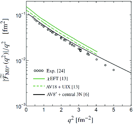
Figure 1: Transition mass form factor $|{\widetilde{\cal F}}_{{\rm M}0^{+}}(q^{2})|$ divided by $q^{2}$. The observed data are shown by the open circles which are transformed from the open circles for $|{\cal F}_{{\rm M}0^{+}}(q^{2})|^{2}$ given in Figs. 3 and 4 of Ref. Kegel ; the relative error in $|{\cal F}_{{\rm M}0^{+}}(q^{2})|^{2}$ is $4\%\!-\!6\%$ except for 11% at the lowest $q^{2}$. The black line represents the calculated form factor provided by Hiyama et al. second2004 using the AV8^′+central 3N potential. The green line (green dashed line) was derived by Bacca et al. Bacca2013 using the $\chi$EFT (AV18+UIX) potential; the lines are transformed from the corresponding lines in Figs. 3 and 4 of Ref. Kegel .

The black line represents the form factor provided by Hiyama et al. second2004 using the AV8^′+central 3N potential. Bacca et al. Bacca2013 derived the green line (green dashed line) using the $\chi$EFT (AV18+UIX) potential; the lines are transformed from the corresponding lines in Figs. 3 and 4 of Ref. Kegel .

In Fig. 2, the observed data are simulated by the blue line which is transformed from the blue line in Figs. 3 and 4 of Ref. Kegel . By virtue of the semi-log plot of Fig. 2, we find that the blue line $(0\leq q^{2}\leq 5.5\,{\rm fm}^{-2})$ is well simulated by a sum of two “straight lines”, namely,

$${\widetilde{\cal F}}_{{\rm M}0^{+}}(q^{2})/q^{2}=a_{1}e^{-b_{1}q^{2}}+a_{2}\,e^{-b_{2}q^{2}}$$ (2)

with $(a_{1},\,a_{2})=(0.092,\,0.035)$ fm² and $(b_{1},\,b_{2})=(0.54,\,2.5)$ fm², which is illustrated in Fig. 2 by the red line; here we fitted the parameters to two significant figures taking the error of the observed data into consideration. This makes it possible to derive a transition mass density from the observed transition form factor as is discussed below.

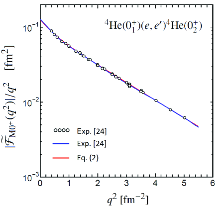
Figure 2: Transition mass form factor $|{\widetilde{\cal F}}_{{\rm M}0^{+}}(q^{2})|$ divided by $q^{2}$. The observed data Kegel are shown by the open circles that are the same as those in Fig. 1. The data are fitted by the blue line, which is transformed from the blue line (the spline polynomial fit function) in Figs. 3 and 4 of Ref. Kegel , whereas the red line shows $|{\widetilde{\cal F}}_{{\rm M}0^{+}}(q^{2})|/q^{2}$ approximated by Eq. (2).

Monopole mass transition density $\rho_{\rm tr}(r)$ is defined as

$$\rho_{\rm tr}(r)=\langle 0^{+}_{2}\,|\frac{1}{4}\sum_{i=1}^{4}\delta({\bf r}-{\bf r}_{i})|\,0^{+}_{1}\rangle,$$ (3)

where the $|\,0^{+}_{1}\rangle$ and $|\,0^{+}_{2}\rangle$ are the four-nucleon wave functions (cf. Eq. (2.1) in Ref. second2004 ), and ${\bf r}_{i}$ is the position vector of $i$th nucleon with respect to the center-of-mass of the four nucleons. This definition is the same as that in Bacca et al. Bacca2015 in their Eq. (9) and Fig. 1. We have

$$\int\,\rho_{\rm tr}(r)\,{\rm d}{\bf r}=0$$ (4)

because the left hand side is the overlap $\langle 0^{+}_{2}\,|\,0^{+}_{1}\rangle$ between the $0^{+}_{1}$ and $0^{+}_{2}$ states.

The form factor ${\widetilde{\cal F}}_{{\rm M}0^{+}}(q^{2})$ is related to the monopole transition density $\rho_{\rm tr}(r)$ as follows:

$${\widetilde{\cal F}}_{{\rm M}0^{+}}(q^{2})=\int e^{i{\bf q}\cdot{\bf r}}\,\rho_{\rm tr}(r)\,{\rm d}{\bf r}.$$ (5)

The density $\rho_{\rm tr}(r)$ can be derived as

$$\rho_{\rm tr}(r)=\frac{1}{(2\pi)^{3}}\int e^{-i{\bf q}\cdot{\bf r}}\,{\widetilde{\cal F}}_{{\rm M}0^{+}}(q^{2})\,{\rm d}{\bf q}$$ (6)

if ${\widetilde{\cal F}}_{{\rm M}0^{+}}(q^{2})$ is provided for all $q^{2}$-range.

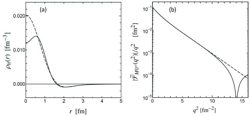
Figure 3: The solid line in (a) illustrates the calculated mass transition mass density $\rho_{\rm tr}(r)$ in Ref. second2004 , which yields the solid-line form factor in (b). The dashed-line form factor in (b) generates the dashed-line density with no central depression in (a).

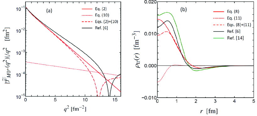
Figure 4: (a) The red solid line is the form factor given by Eq. (2). The red dotted line is the absolute value of example additional form factor Eq. (10) for the central depression of the transition density. The red dashed line denotes the example form factor, Eq. (2) plus Eq. (10), generating the central depression. The black line is the form factor given by Ref. second2004 . (b) The red solid line denotes the transition density Eq. (8). The red dotted line represents the example additional density Eq. (11) for simulating central depression. The red dashed line denotes the example density, Eq. (8) plus Eq. (11), having central depression. The black line is the density given in Fig. 2b of Ref. second2004 . The green line denotes the density calculated using the $\chi$EFT potential given in Fig. 1 of Ref. Bacca2015 .

We examined whether extending Eq. (2) to the range of $q^{2}>5.5$ fm^-2 is meaningful. As a test example, we employed $\rho_{\rm tr}(r)$ and ${\widetilde{\cal F}}_{{\rm M}0^{+}}(q^{2})$ calculated in Ref. second2004 . The density $\rho_{\rm tr}(r)$ $(=\rho_{00}(r)/\sqrt{4\pi}$ second2004 ) is illustrated in Fig. 3a by the solid line with a node at $r=1.62$ fm, whereas $|{\widetilde{\cal F}}_{{\rm M}0^{+}}(q^{2})|/q^{2}$ is shown in Fig. 3b as a solid line with a node at $q^{2}=14.1\,{\rm fm}^{-2}$ $({\widetilde{\cal F}}_{{\rm M}0^{+}}(q^{2})=\sqrt{4\pi}F_{\rm inel}(q^{2})$ second2004 ). The solid-line form factor in the range of $3<q^{2}<5.5\,{\rm fm}^{2}$ extends to $5.5<q^{2}<9\,{\rm fm}^{2}$ to maintain similar decay rates. We approximated the solid-line form factor, as shown in Fig. 3b in the range of $3<q^{2}<9\,{\rm fm}^{-2}$ using the function

$${\widetilde{\cal F}}_{{\rm M}0^{+}}(q^{2})/q^{2}=a_{0}\,e^{-b_{0}q^{2}}$$ (7)

with $a_{0}=0.078\,{\rm fm}^{2}$ and $b_{0}=0.45\,{\rm fm}^{2}$, and extended it to the range $q^{2}>9\,{\rm fm}^{-2}$, as indicated by the dashed line in Fig. 3b; in the range of $q^{2}<9\,{\rm fm}^{-2}$, the dashed line was considered the same as the solid line. We substitute the dashed-line form factor into Eq. (6) and obtain the dashed-line density in Fig. 3a with a node at $r=1.66$ fm. The difference between the solid- and dashed-line form factors in the range of $q^{2}>9\,{\rm fm}^{-2}$ in Fig. 3b appears as a central depression at $r\lesssim 1$ fm on the solid-line density in Fig. 3a, and generates only a small difference in the density for $r\gtrsim 1$ fm. Subsequently, we considered that an extension of Eq. (2) to the range of $q^{2}>5.5$ fm^-2 will be useful for studying the observed form factor.

We extend the form factor Eq. (2) in the range of $q^{2}>5.5\,{\rm fm}^{-2}$, as illustrated in Fig. 4a by the red solid line. Using the form factor in Eq. (2) over the entire $q^{2}$ range, we obtain

$$\rho_{\rm tr}(r)=A_{1}\left(3-\tfrac{1}{2b_{1}}r^{2}\right)\,e^{-\frac{1}{4b_{1}}r^{2}}+A_{2}\left(3-\tfrac{1}{2b_{2}}r^{2}\right)\,e^{-\frac{1}{4b_{2}}r^{2}}$$ (8)

where

$$A_{1}=\frac{a_{1}}{(2\pi)^{3}}\frac{1}{2b_{1}}\left(\frac{\pi}{b_{1}}\right)^{3/2},\qquad A_{2}=\frac{a_{2}}{(2\pi)^{3}}\frac{1}{2b_{2}}\left(\frac{\pi}{b_{2}}\right)^{3/2}$$ (9)

with $A_{1}=4.8\times 10^{-2}\;{\rm fm}^{-3}$ and $A_{2}=4.0\times 10^{-5}\;{\rm fm}^{-3}$. The density $\rho_{\rm tr}(r)$ of Eq. (8) is shown in Fig. 4b using the solid red line with a node at $r=1.82$ fm, which is almost the same node position as that of the dominant first term in Eq. (8) at $r=\!\sqrt{6b_{1}}=1.80$ fm. For comparison, we show in Fig. 4b the transition density given by Hiyama et al. second2004 by the black line calculated using the AV8^′ + central 3N potential and that given by Bacca et al. Bacca2015 by the green line calculated using the $\chi$EFT interaction (extracted from Fig. 1 Bacca2015 ).

3. Central depression of transition density

We focus on the central depression of the transition density $\rho_{\rm tr}(r)$ in Fig. 4b in the range of $r\lesssim 1$ fm as indicated by the black line second2004 and the green line Bacca2015 . As shown above, the red-solid-line density with no central depression in Fig. 4b is generated by the red-solid-line form factor in Fig. 4a. We then attempt to provide an artificial example of a central depression to the red-solid-line density. We considered a small additional transition form factor $\Delta{\widetilde{\cal F}}_{{\rm M}0^{+}}(q^{2})$,

$$\Delta{\widetilde{\cal F}}_{{\rm M}0^{+}}(q^{2})/q^{2}=a_{3}\,e^{-b_{3}q^{2}},$$ (10)

which is related to an additional transition density $\Delta\rho_{\rm tr}(r)$ (note $\int\!\Delta\rho_{\rm tr}(r)\,{\rm d}{\bf r}=0$)

$$\Delta\rho_{\rm tr}(r)=A_{3}\left(3-\tfrac{1}{2b_{3}}r^{2}\right)\,e^{-\tfrac{1}{4b_{3}}r^{2}}$$ (11)

with

$$A_{3}=\frac{a_{3}}{(2\pi)^{3}}\frac{1}{2b_{3}}\left(\frac{\pi}{b_{3}}\right)^{3/2}.$$ (12)

We consider, as an example, $a_{3}=-0.00037$  fm² and $b_{4}=0.090\,{\rm fm}^{2}$, yielding $A_{4}=-0.0017\,{\rm fm}^{-3}$. $\Delta{\widetilde{\cal F}}_{{\rm M}0^{+}}(q^{2})/q^{2}$ and $\Delta\rho_{\rm tr}(r)$ are presented in Fig. 4a and 4b, respectively, indicated by the red dotted line. The summed form factor $({\widetilde{\cal F}}_{{\rm M}0^{+}}(q^{2})+\Delta{\widetilde{\cal F}}_{{\rm M}0^{+}}(q^{2}))/q^{2}$ is shown in Fig. 4a by a red dashed line with a node at $q^{2}=12.2\,{\rm fm}^{-2}$. The transition density $\rho_{\rm tr}(r)+\Delta\rho_{\rm tr}(r)$ is illustrated in Fig. 3b by the red dashed line, which is close to the red-solid line $\rho_{\rm tr}(r)$ within the range of $r\gtrsim 1$ fm.

The central-depression phenomena of the transition density originates from the behavior of the form factor in the range of $q^{2}\gtrsim 10$ fm^-2, and the observed transition form factor Kegel limited to the range of $q^{2}\leq 5\,{\rm fm}^{-2}$ cannot provide information about the central-depression structure at $r\lesssim 1$ fm. However, we considered that using the observed form factor can be used to derive the transition density $\rho_{\rm tr}(r)$ in the range $r\gtrsim 1$ fm, as indicated in Fig. 4b by the solid and dashed red lines, which is significantly different from the black and green lines ($r\gtrsim 1$ fm) obtained in the literature second2004 ; Bacca2013 .

4. Monopole matrix element $\langle r^{2}\rangle_{\rm tr}$ and transition radius $\mathcal{R}_{\rm tr}$

As important information on the spatial structure of the second $0^{+}$ state, the authors of Ref. Kegel extracted, from the observed form factor, the monopole matrix element $\langle r^{2}\rangle_{\rm tr}$ and the transition radius $\mathcal{R}_{\rm tr}$ defined as (cf. Eq. (5) in Ref. Kegel )

$$\langle r^{n}\rangle_{\rm tr}=Z\left|\,\!\int r^{n}\,\rho_{\rm tr}(r)\,{\rm d}{\bf r}\,\right|\quad(n=2\,\,{\rm and}\,\,4,Z=2),\qquad\mathcal{R}_{\rm tr}^{2}=\frac{\langle r^{4}\rangle_{\rm tr}}{\langle r^{2}\rangle_{\rm tr}},$$ (13)

which are obtained by a ${\bf q}\to 0$ expansion of the form factor

$$Z\,|{\widetilde{\cal F}}_{{\rm M}0^{+}}(q^{2})|/q^{2}=\tfrac{1}{6}\langle r^{2}\rangle_{\rm tr}-\tfrac{1}{120}\langle r^{4}\rangle_{\rm tr}\,q^{2}+{\cal O}(q^{4}),$$ (14)

with $e^{i{\bf q}\cdot{\bf r}}\to 1-\tfrac{1}{6}q^{2}r^{2}+\tfrac{1}{120}q^{4}r^{4}+\cdot\cdot\cdot$ for the “monopole” density $\rho_{\rm tr}(r)$ in Eq. (5). They determined the numerical values of $\langle r^{2}\rangle_{\rm tr}$ and $\mathcal{R}_{\rm tr}$, as indicated by the first line in Table I.

We calculate $\langle r^{2}\rangle_{\rm tr}$ and $\mathcal{R}_{\rm tr}$ in Eq. (14) explicitly using the red-solid-line density, Eq (8), with no central depression and the red-dashed-line density, Eq.(8) plus Eq. (11), with central depression. We obtain, for the red-dashed-line density,

$$\langle r^{2}\rangle_{\rm tr}=6\,Z\,|\,a_{1}+a_{2}+a_{3}\,|,\qquad\langle r^{4}\rangle_{\rm tr}=120\,Z\,|\,a_{1}b_{1}+a_{2}b_{2}+a_{3}b_{3}\,|,$$ (15)

where $a_{3}$ and $b_{3}$ are omitted in the case of the red-solid-line density. The numerical values of $\langle r^{2}\rangle_{\rm tr}$ and $\mathcal{R}_{\rm tr}$ are listed in Table I. The two transition densities reproduce the experimental value; however, this is natural because the form factors of Eqs. (2) and (10) are constructed to simulate the behavior of the observed form factor (blue line) at $q^{2}\sim 0$. As expected, the central-depression structure is not reflected in $\langle r^{2}\rangle_{\rm tr}$ and $\mathcal{R}_{\rm tr}$ (that is, the contributions of $a_{3}$ and $b_{3}$ are negligible in Eq. (15)).

Table 1:    Values of $\langle r^{2}\rangle_{\rm tr}$ and $\mathcal{R}_{\rm tr}$.

		$\langle r^{2}\rangle_{\rm tr}\,({\rm fm}^{2})$		$\mathcal{R}_{\rm tr}\,({\rm fm})$
Experiment, Ref. Kegel		$1.53\pm 0.05$		$4.56\pm 0.15$
Red-solid-line density, Eq. (8)		$1.52$		$4.65$
Red-dashed-line density, Eqs. (8) plus (11)		$1.52$		$4.65$

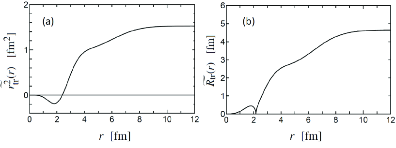
Figure 5: (a) Cumulative monopole matrix element ${\widetilde{r^{2}_{\rm tr}}}(r)$ and (b) Cumulative transition density ${\widetilde{\mathcal{R}_{\rm tr}}}(r)$ defined by Eq. (16). In each of (a) and (b), the lines for the red-solid-line and red-dashed-line densities in Fig. 4b overlap within the thickness of the lines. Here, ${\widetilde{r^{2}_{\rm tr}}}(\infty)=\langle r^{2}\rangle_{\rm tr}=1.52\,{\rm fm}^{2}$ and ${\widetilde{\mathcal{R}_{\rm tr}}}(\infty)=\mathcal{R}_{\rm tr}=4.65\,{\rm fm}^{-2}$ (cf. Table I).

To investigate the range of $r$ that contributes most to $\langle r^{2}\rangle_{\rm tr}$ and $\mathcal{R}_{\rm tr}$, we introduce the cumulative monopole matrix element ${\widetilde{r^{2}_{\rm tr}}}(r)$ and the cumulative transition density ${\widetilde{\mathcal{R}_{\rm tr}}}(r)$ as a function of $r$ by

$${\widetilde{r^{2}_{\rm tr}}}(r)\equiv 4\pi Z\left|\int_{0}^{\,r}\!{r^{\prime}}^{2}\rho_{\rm tr}({r^{\prime}})\,r^{\prime 2}{\rm d}{r^{\prime}}\,\right|,\qquad{\widetilde{\mathcal{R}_{\rm tr}}}(r)\equiv\left|\,\frac{4\pi Z}{\langle r^{2}\rangle_{\rm tr}}\int_{0}^{\,r}\!r^{\prime 4}\rho_{\rm tr}(r^{\prime})\,r^{\prime 2}{\rm d}r^{\prime}\,\right|^{1/2},$$ (16)

where ${\widetilde{r^{2}_{\rm tr}}}(\infty)=\langle r^{2}\rangle_{\rm tr}$ and ${\widetilde{\mathcal{R}_{\rm tr}}}(\infty)=\mathcal{R}_{\rm tr}$. The functions ${\widetilde{r^{2}_{\rm tr}}}(r)$ and ${\widetilde{\mathcal{R}_{\rm tr}}}(r)$ are shown in Figs. 5a and 5b, respectively. In both cases, the dominant contribution comes from the range of $r\gtrsim 3$ fm. Interestingly, this part appears to be minor in the region of Fig. 4b for the transition density. We understand that we must derive the transition density $\rho_{\rm tr}(r)$ up to $r\!\sim\!10$ fm so that $\langle r^{2}\rangle_{\rm tr}$ and $\mathcal{R}_{\rm tr}$ are calculated accurately.

5. Discussions

We have derived a possible $0^{+}_{1}\!\to\!0_{2}^{+}$ transition density $\rho_{\rm tr}(r)$ for $r\gtrsim 1$ fm as in Fig. 4b by the solid red line except for the inner central-depression region, utilizing the information obtained from the newly observed high-precision transition form factor for $0\leq q^{2}\leq 5\,{\rm fm}^{-2}$ Kegel . The shape of the transition density is significantly different from those obtained theoretically in literature second2004 ; Bacca2013 .

We now discuss a problem calculating the energy of the second $0^{+}$ state. Figure 6 schematically illustrates the energy values obtained using the AV8^′+central 3N potential second2004 and by the $\chi$EFT and AV18+UIX potentials Bacca2013 along with the threshold energies of the $\,{}^{3}{\rm H}+p$, ${}^{3}{\rm He}+n$ and their average $3N+N$ configurations Tilley1992 . Note that the observed $0^{+}_{2}$ state is located between the ${}^{3}{\rm H}+p$ and ${}^{3}{\rm He}+n$ thresholds and only 0.01 MeV above the $3N+N$ threshold with a rather narrow width of $\Gamma_{\rm p}=0.50$ MeV Tilley1992 for a $S$-wave resonance.

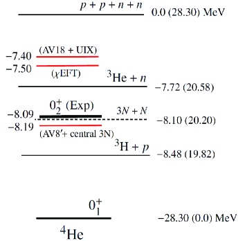
Figure 6: Schematic illustration of the $0^{+}_{2}$ energy obtained using the AV8^′+central 3N potential Ref. second2004 and by the AV18+UIX and $\chi$EFT potentials Bacca2013 along with the threshold energies of the ${}^{3}{\rm H}+p$, ${}^{3}{\rm He}+n$, their averaged $3N+N$, and $p+p+n+n$ configurations Tilley1992 .

In Ref. second2004 which took the isospin-formalism, the $0^{+}_{2},T\!=\!0$ state was obtained only 0.1 MeV below the observed level as a bound state measured from the $3N+N$ threshold. On the other hand, in Ref. Bacca2013 , the energy of the $0^{+}_{2}$ state obtained as a resonance with the two realistic interactions is $\sim\!0.7$ MeV above the observed $0^{+}_{2}$ level and even above the ${}^{3}{\rm He}+n$ threshold. As mentioned by Bacca et al. Bacca2013 and Epelbaum Epelbaum , it is possible that the improper theoretical resonance position affects the form factor result. As pointed by Horiuchi and Suzuki (cf. last paragraph of Sec. IIIB of Ref. Horiuchi ), the observed $0^{+}_{2}$ state is considered a Feshbach resonance embedded in the ${}^{3}{\rm H}+p$ continuum as a bound state with respect to the ${}^{3}{\rm He}+n$ threshold.

In the opinion of the present author, a possible strategy to attack the $\alpha$-particle monopole puzzle using fully realistic interactions is as follows: (i) Solve the $0^{+}_{2}$ state using the bound-state approximation to search interaction parameters that reproduce the $0^{+}_{2}$ energy as well as the binding energies of ${}^{3}{\rm H}$, ${}^{3}{\rm He}$ and ${}^{4}{\rm He}$, (ii) calculate the transition density and form factor, and then (iii) solve the ${}^{3}{\rm H}+p$ scattering to derive the wave function and width of the Feshbach resonance as well as the final results for the transition density and form factor.

As mentioned in Sec. 1, authors of Ref. Kegel claimed the following: the large difference between the calculated form factors does not stem from numerical methods but from the Hamiltonian. However, the comparison between the methods was performed only for the calculation based on the bound-state approximation. The calculation of the $0^{+}_{2}$ state as a resonance was performed using only the LIT approach. For example, it would be desirable to examine this problem by the comparison with the form factor results produced by using any explicit four-body ${}^{3}{\rm H}+p$ scattering calculation such as Ref. Viviani2020 .

Acknowledgements

The author would like to thank Dr. S. Kegel for providing with the numerical values of the experimental data of Ref. Kegel and valuable discussions on the data. This work is supported by the Grant-in-Aid for Scientific Research on Innovative Areas, “Toward new frontiers: Encounter and synergy of state-of-the-art astronomical detectors and exotic quantum beams”, Grant Number 18H05461.

References

- (1) H. Kamada, A. Nogga, W. Glöckle, E. Hiyama, M. Kamimura, K. Varga, Y. Suzuki, M. Viviani, A. Kievsky, S. Rosati, J. Carlson, S. C. Pieper, R. B. Wiringa, P. Navratil, B. R. Barrett, N. Barnea, W. Leidemann, and G. Orlandini, Phys. Rev. C 64, 044001 (2001).
- (2) B. S. Pudliner, V. R. Pandharipande, J. Carlson, S. C. Pieper, and R. B. Wiringa, Phys. Rev. C 56, 1720 (1997).
- (3) M. Kamimura, Phys. Rev. A38, 621 (1988).
- (4) H. Kameyama, M. Kamimura and Y. Fukushima, Phys. Rev. C 40, 974 (1989).
- (5) E. Hiyama, Y. Kino and M. Kamimura, Prog. Part. Nucl. Phys. 51, 223 (2003).
- (6) E. Hiyama, B.F. Gibson, and M. Kamimura, Phys. Rev. C 70, 031001(R) (2004).
- (7) R. F. Frosch, R. E. Rand, H. Crannell, J. S. McCarthy, L. R. Suelzle, and M. R. Yearian, Nucl. Phys. A110, 657 (1968).
- (8) Th. Walcher, Phys. Lett. B, 31, 442 (1970).
- (9) G. Koebschall, C. Ottermann, K. Maurer, K. Roehrich, Ch. Schmitt and V. H. Walther, Nucl. Phys. A405, 648 (1983).
- (10) W. Horiuchi and Y. Suzuki, Phys. Rev. C 78, 034305 (2008).
- (11) Y. Suzuki and K. Varga, Stochastic Variational Approach to Quantum Mechanical Few-Body Problems (Springer-Verlag, Berlin, 1998).
- (12) K. Varga and Y. Suzuki, Phys. Rev. C 52, 2885 (1995).
- (13) S. Bacca, N. Barnea, W. Leidemann, and G. Orlandini, Phys. Rev. Lett. 110, 042503, (2013).
- (14) S. Bacca, N. Barnea, W. Leidemann, and G. Orlandini, Phys. Rev. C 91, 024303, (2015).
- (15) N. Barnea and A. Novoselsky, Phys. Rev. A 57, 48 (1998).
- (16) N. Barnea, W. Leidemann, and G. Orlandini, Phys. Rev. C 61, 054001 (2000).
- (17) V.D. Efros, W. Leidemann, and G. Orlandini, Phys. Lett. B 338, 130 (1994).
- (18) V.D. Efros, W. Leidemann, G. Orlandini, and N. Barnea, J. Phys. G 34, R459 (2007).
- (19) R.B. Wiringa, V.G.J. Stoks, and R. Schiavilla, Phys. Rev. C 51, 38 (1995).
- (20) B.S. Pudliner, V. Pandharipande, J. Carlson, and R. Wiringa, Phys. Rev. Lett. 74, 4396 (1995).
- (21) D. R. Entem and R. Machleidt, Phys. Rev. C 68, 041001(R) (2003).
- (22) P. Navratil, Few-Body Syst. 41, 117 (2007).
- (23) D. Gazit, S. Quaglioni, and P. Navratil, Phys. Rev. Lett. 103, 102502 (2009).
- (24) S. Kegel et al., Phys. Rev. Lett. 130, 152502, (2023).
- (25) E. Epelbaum, Physics 16, 58 (2023).
- (26) D.R. Tilley, H.R. Weller, and G.M.Hale, Nucl. Phys. A 541, 1 (1992).
- (27) M. Viviani, L. Girlanda, A. Kievsky, and L.E. Marcucci, Phys. Rev. C 102, 034007 (2020).