Diffusion Models for Black-Box Optimization

Abstract

The goal of offline black-box optimization (BBO) is to optimize an expensive black-box function using a fixed dataset of function evaluations. Prior works consider forward approaches that learn surrogates to the black-box function and inverse approaches that directly map function values to corresponding points in the input domain of the black-box function. These approaches are limited by the quality of the offline dataset and the difficulty in learning one-to-many mappings in high dimensions, respectively. We propose Denoising Diffusion Optimization Models (DDOM), a new inverse approach for offline black-box optimization based on diffusion models. Given an offline dataset, DDOM learns a conditional generative model over the domain of the black-box function conditioned on the function values. We investigate several design choices in DDOM, such as reweighting the dataset to focus on high function values and the use of classifier-free guidance at test-time to enable generalization to function values that can even exceed the dataset maxima. Empirically, we conduct experiments on the Design-Bench benchmark (Trabucco et al., 2022) and show that DDOM achieves results competitive with state-of-the-art baselines. Our implementation of DDOM can be found at https://github.com/siddarthk97/ddom.

1.4pt

1 Introduction

Many fundamental problems in science and engineering involve optimization of an expensive black-box function, such as optimal experimental design and product optimization. Since evaluating the black-box function is expensive, recent works consider purely data-driven approaches that use only offline logged datasets to optimize the target function sidestepping real-world interactions (Trabucco et al., 2021; Kumar & Levine, 2020; Hansen, 2016). We refer to this paradigm as offline black-box optimization (BBO).

Figure 1: Schematic for DDOM. We train our conditional diffusion model using a reweighted objective function. During testing, we condition on the maximum $y$ in the dataset and use classifier-free guidance to sample $Q$ candidate points.

The key challenge for offline BBO is the limited coverage of the offline dataset. Accordingly, there are two broad classes of approaches in prior works. Following the tradition of online BBO, many forward approaches learn a surrogate model mapping inputs to their function values. Once learned, this surrogate can be optimized with respect to its input using a gradient-based optimizer or serve as a proxy oracle for a standard online BBO surrogate e.g., BayesOpt using a Gaussian Process. Forward approaches are indirect, and learning a surrogate that generalizes outside the offline dataset can be challenging (Trabucco et al., 2021).

In contrast, inverse approaches directly learn a mapping from function values to inputs in the domain of the black-box function. This mapping is generally one-to-many as many points can have the same function value. The key advantage of an inverse model is that at test time, we can simply condition the model on high/low function values to obtain candidate optima. However, learning one-to-many mappings is challenging, especially when the underlying black-box function is defined over a high-dimensional domain. Prior works have found some success with generative approaches based on generative adversarial networks (GAN) (Kumar & Levine, 2020; Goodfellow et al., 2014; Mirza & Osindero, 2014). These approaches inherit the problem of their base models, such as training instability and mode collapse for GANs.

We develop a new approach called Denoising Diffusion Optimization Models (DDOM) that uses conditional diffusion models (Ho et al., 2020; Song et al., 2020, 2021; Huang et al., 2021) to parameterize and learn the inverse mapping. A diffusion model specifies an encoding-decoding procedure based on adding small amounts of noise over multiple timesteps during encoding and then reconstructing the original signal based on the noisy encodings during the decoding stage (Sohl-Dickstein et al., 2015). Diffusion models have shown excellent success across a range of continuous data, such as images (Song et al., 2021, 2020; Ho et al., 2020), videos (Ho et al., 2022), and speech (Kim et al., 2022; Jeong et al., 2021; Kong et al., 2021). They also allow for conditioning on other inputs, and as a result, they also define flexible models that map one modality to another, such as text2image models (Saharia et al., 2022; Ramesh et al., 2021). For offline BBO in DDOM, we condition the diffusion model over the observed function values.

We investigate various design choices that enable successful learning for DDOM. In particular, we find there are 2 critical tradeoffs in applying DDOM for offline BBO. First, even though the offline datapoints are assumed to be sampled i.i.d., we want to specifically condition the model on large values at test-time. This creates a bias-variance tradeoff where we need to prioritize high value datapoints over others (Kumar & Levine, 2020). We resolve this tradeoff by optimizing a weighted loss that downweights the evidence lower bound due to low quality datapoints.

Second, we build on the observation that conditional diffusion models exhibit a diversity-quality tradeoff (Dhariwal & Nichol, 2021). In emphasizing for diverse candidates, a diffusion model can ignore or downplay the conditioning information. This is detrimental for offline BBO which explicitly relies on conditioning as a means of optimization at test-time. Following Ho & Salimans (2021), we fix this issue by decomposing the score function into an unconditional and conditional component. By adjusting the weights of the two components at test-time, we can generate candidates for the optima that explicitly prioritize the conditioning information, as desired.

Empirically, we test DDOM on the Design-Bench suite (Trabucco et al., 2022) of tasks for offline BBO. The suite contains a variety of real-world domains spanning both discrete and continuous domains and a variety of data sizes and dimensionalities. We find that DDOM is very stable to train and performs exceedingly well on this suite. Specifically, DDOM outperforms all the forward and inverse baselines achieving the highest rank on average (2.8).

2 Background

2.1 Problem Statement

Let $f:\mathcal{X}\rightarrow\mathbb{R}$ denote the unknown black-box function, where the domain $\mathcal{X}$ is an arbitrary subset of $\mathbb{R}^{d}$. The black-box optimization problem involves finding a point $\mathbf{x}^{*}$ that maximizes $f$:

$$\mathbf{x}^{*}\in\mathop{\mathrm{argmax}}_{\mathbf{x}\in\mathcal{X}}f(\mathbf{x})$$

We operate in the setting of offline BBO (Trabucco et al., 2022), where we are not allowed to evaluate $f(\mathbf{x})$ for any $\mathbf{x}$ during training, but must instead make use of an offline dataset of points, which we denote by $\mathcal{D}=\{(\mathbf{x}_{1},y_{1}),(\mathbf{x}_{2},y_{2}),\cdots,(\mathbf{x}_{n},y_{n})\}$. We are allowed a small budget of $Q$ queries during the evaluation to output candidates for the optimal point.

2.2 Diffusion Models

Diffusion models are a class of latent-variable deep generative models that parameterize the encoding and decoding processes via a diffusion process. The core idea behind diffusion is to add small amounts of noise iteratively to a sample, and train a neural network to invert the transformation. In our work, we make use of continuous time diffusion models (Song et al., 2021; Huang et al., 2021).

Let $\mathbf{x}_{t}$ denote a random variable signifying the state of a data point $\mathbf{x}_{0}$ at time $t$ where $t\in[0,T]$. We assume $\mathbf{x}_{0}$ is sampled from some unknown data distribution $p_{0}(\mathbf{x})$ and $\mathbf{x}_{T}$ represent points sampled from some prior noise distribution (e.g., standard normal distribution). The forward diffusion process can then be defined as a stochastic differential equation (SDE):

$$d\mathbf{x} =\mathbf{f}(\mathbf{x},t)dt+g(t)d\mathbf{w}$$ (1)

where $\mathbf{w}$ is the standard Wiener process, $\mathbf{f}:\mathbb{R}^{d}\rightarrow\mathbb{R}^{d}$ is the drift coefficient, and $g(t):\mathbb{R}\rightarrow\mathbb{R}$ is the diffusion coefficient of $\mathbf{x}_{t}$.

The reverse time process (a.k.a. denoising) maps noise to data and can also be defined using an SDE:

$$d\mathbf{x} =[\mathbf{f}(\mathbf{x},t)-g(t)^{2}\nabla_{\mathbf{x}}\log p_{t}(\mathbf{x})]dt+g(t)d\tilde{\mathbf{w}}$$ (2)

where $dt$ is an infinitesimal step backwards in time, and $d\tilde{\mathbf{w}}$ is a reverse time Wiener process. In practice, the score function $\nabla_{\mathbf{x}}\log p_{t}(\mathbf{x})$ is estimated by a time-dependent neural network $\epsilon_{\theta}(\mathbf{x}_{t},t)$ trained using a score matching objective such as denoising score matching (Vincent, 2011).

2.3 Classifier-free Guidance

In this work, we are interested in training a conditional diffusion model. In practice, naively conditioning a standard diffusion model by appending the conditioned variable at each step of the denoising process does not work well as the model often ignores or downplays the conditioning information during practice. One mitigation strategy is based on classifier-free diffusion (Ho & Salimans, 2021), where we decompose the score function into a linear combination of a conditional and an unconditional score function:

$$\epsilon_{\theta}(\mathbf{x},t,y)=(1+\gamma)\epsilon_{\texttt{cond}}(\mathbf{x},t,y)-\gamma\epsilon_{\texttt{uncond}}(\mathbf{x},t)$$ (3)

Here, the mixing parameter $\gamma$ acts as a trade-off between coverage and fidelity while sampling. For $\gamma=-1$, the score function translates to sampling from an unconditional diffusion model. For $\gamma\geq 0$, the score function prioritizes samples that strongly respect the conditioning information. Classifier-free guidance obviates the need for training a model on the noisy diffusion data. In practice, instead of learning two separate models for the unconditional and conditional score function, we can train a single model to estimate both by randomly setting the conditioning value to zero during training.

3 Denoising Diffusion Optimization Models

We are interested in learning an inverse model ($y$ to $\mathbf{x}$ mapping) for offline BBO.Since $\mathbf{x}$ is typically high-dimensional, the learned mapping is one-to-many. We can parameterize any one-to-many mapping as a conditional probability distribution $p(\mathbf{x}|y)$ such that conditioned on a specific value of $y$, the support of the distribution is concentrated on all datapoints $\mathbf{x}$ for which $f(\mathbf{x})\sim y$.

In recent years, deep generative models have shown to excel at learning high-dimensional probability distributions. For offline BBO, any generative model could be used in principle and related works have explored approaches inspired via generative adversarial networks (Goodfellow et al., 2014; Kumar & Levine, 2020). However, similar to GANs, these BBO approaches are generally hard to train and can also suffer from mode collapse, wherein the sampled points are all very similar. In this work, we propose to use Diffusion Models for learning the inverse mapping (Sohl-Dickstein et al., 2015). Diffusion models have surpassed GANs for many domains, such as image synthesis (Dhariwal & Nichol, 2021). Moreover, they have novel controls for conditional generation, such as guidance, which explicitly allows for trading sample diversity for conditioning. We refer to our proposed models as Denoising Diffusion Optimization Models (DDOM).

Training via Loss Reweighting Formally, we train a conditional diffusion model on the offline dataset $\mathcal{D}$. During the forward diffusion, we use an SDE with a Variance Preserving (VP) noise perturbation (Song et al., 2021). Concretely, our forward SDE looks like the following:

$$d\mathbf{x}=-\frac{1}{2}\beta_{t}dt+\sqrt{\beta_{t}}d\mathbf{w}$$ (4)

where $\beta_{t}=\beta_{\texttt{min}}+(\beta_{\texttt{max}}-\beta_{\texttt{min}})t$ and $t\in[0,1]$. We instantiate the surrogate model for the score function using a simple feed-forward neural network conditioned on the time $t$ and value $y$. It has been shown previously that a discretization of the above SDE corresponds to the forward diffusion in DDPM (Song et al., 2021; Ho et al., 2020).

A naive optimization of the denoising objective would sample $(\mathbf{x},y)$ pairs uniformly from the offline dataset. However, we note that since our end goal is to find the argument maximizing $y$, it is important for our model to perform well on relatively high values of $y$. Filtering out suboptimal $y$ is data inefficient as there could be a learning signal present even when $y$ is low. Instead, we pursue a reweighting strategy similar to Kumar & Levine (2020). We partition the offline dataset $\mathcal{D}$ into $N_{B}$ bins of equal width over $y$. Then for each bin, we assign a weight proportional to the number of points in the bin and the average value of the points in the bin. This ensures that we assign a higher weight during training to (i) bins with more points and (ii) bins with better points (points with higher $y$ on average). Concretely the weight $w_{i}$ for bin $i$ can be computed as:

$$w_{i}=\frac{|B_{i}|}{|B_{i}|+K}\exp{\left(\frac{-|\hat{y}-y_{b_{i}}|}{\tau}\right)}$$ (5)

where $\hat{y}$ is the best function value in the offline dataset $\mathcal{D}$, $|B_{i}|$ refers to the number of points in the $i^{th}$ bin, and $y_{b_{i}}$ is the midpoint of the interval corresponding to the bin $B_{i}$. The parameters $K$ and $\tau$ are hyper-parameters, and more details on them can be found in Appendix B.

We finally optimize the objective

where $w(y)=w_{i}$ if $y\in B_{i}$. Notice the extra reweighting terms introduced here are dependent on $y$ (but independent of $t$ and complementary to the original time-dependent weighting $\lambda(t)$.

During training, we normalize the dimensions of the data points and function values to fit a standard normal. For discrete tasks, we can train a VAE to project the inputs to a continuous domain. However, we map the inputs to log probabilities, following the same procedure as Trabucco et al. (2022). They emulate logit values by interpolating between a uniform distribution and the one hot values (this is equivalent to mapping the one hot values to some other constant non-zero values). We find that this simple procedure performs reasonably well in our experiments.

Testing via Classifier-Free Guidance Once we train the conditional score function, we can use it to generate samples from the reverse SDE. Sampling requires a few design decisions: choosing a conditioning value of $y_{\texttt{test}}$, an estimate for the score function, and an SDE solver. Ideally, we would like to choose a $y$ that corresponds to the optima, i.e., $y^{\star}=f(\mathbf{x}^{\star})$. However, in practice, we do not know $y^{\star}$; hence, we instead propose to set $y_{\texttt{test}}$ to the maximum value of $y$ in the observed dataset $\mathcal{D}$, and by setting the guidance weight to a large value. By doing so, we find that the model can generate points further from the unconditional data distribution. This phenomena is analogous to the use of guidance for image generation where sample fidelity can sometimes exceed even real images (e.g., for art) at the cost of diversity. We also find that in practice, this strategy works well, especially with an adjusted score function estimate based on classifier-free guidance (Equation 3). Finally, we use a second-order Heun solver for sampling from the reverse SDE and find it to work slightly better than first-order solvers in line with recent works (Jolicoeur-Martineau et al., 2021; Karras et al., 2022).

Algorithm 1 Denoising Diffusion Optimization Models

Input Offline dataset $\mathcal{D}$, Query budget $Q$, Smoothing parameter $K$, Temperature $\tau$, Number of bins $N_{B}$
Output A set of proposed candidate points $\mathbf{X}$ with the constraint $|\mathbf{X}|\leq Q$

1:  {Phase $1$: Training}

2:  Construct bins $\{B_{1},\cdots,B_{N_{B}}\}$ from $\mathcal{D}$, each bin covering equal $y$-range

3:  Calculate the weights $(w_{1},w_{2},\cdots,w_{N_{B}})$ for each bin using Equation 5

4:  Initialize the model parameters $\theta$

5:  Train score estimator $\epsilon_{\theta}$ using Equation 6

6:  {Phase $2$: Evaluation }

7:  $y_{\text{test}}\leftarrow\mathrm{max}\{y\mid(x,y)\in\mathcal{D}\}$

8:  $\mathbf{X}\leftarrow\phi$

9:  for $i=1,\cdots,Q$ do

10:     Sample $\mathbf{x}_{T}\sim\mathcal{N}(0,\mathbf{I})$

11:     for $t=T-1,\cdots,0$ do

12:        $\mathbf{x}_{t}\leftarrow\textsc{HEUN-SAMPLER}(\mathbf{x}_{t+1},\theta,y_{\text{test}})$

13:     end for

14:     $\mathbf{X}\leftarrow\mathbf{X}\cup\{x_{0}\}$

15:  end for

16:  return $\mathbf{X}$

4 Experiments

4.1 Toy Branin Task

Branin is a well-known function for benchmarking optimization methods. We consider the negative of the standard 2D Branin function in the range $x_{1}\in[-5,10]$ and $x_{2}\in[0,15]$:

$$f_{br}(x_{1},x_{2})=-a(x_{2}-bx_{1}^{2}+cx_{1}-r)^{2}-s(1-t)\cos{x_{1}}-s$$ (7)

where $a=1$, $b=\frac{5.1}{4\pi^{2}}$, $c=\frac{5}{\pi}$, $r=6$, $s=10$, and $t=\frac{1}{8\pi}$. In this square region, $f_{br}$ has three global maximas, $(-\pi,12.275)$, $(\pi,2.275)$, and $(9.42478,2.475)$; with the maximum value of $-0.397887$ (Figure 2).

Figure 2: Branin function

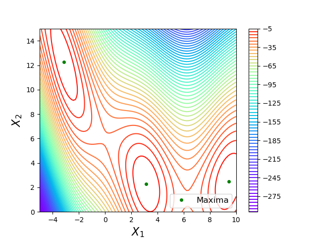
Unconditional Diffusion We first conduct illustrative experiments in an unconditional setting. We emulate an offline dataset that predominantly contains points with high function values and study if DDOM can generate samples from the base distribution.

(a) $\mathcal{D}_{\text{GMM}}$

(b) Sample reverse diffusion trajectory for DDOM trained on $\mathcal{D}_{\text{GMM}}$

(c) Sample statistics

(d) $\mathcal{D}_{\text{Unif}}$

(e) Sample reverse diffusion trajectory for DDOM trained on $\mathcal{D}_{\text{Unif}}$

(f) Sample statistics

Figure 3: Unconditional diffusion model trained on two data distributions. Top row: (a) Dataset distribution of $\mathcal{D}_{\text{GMM}}$. (b) Denoising steps of the diffusion model. (c) Maximum (blue line) and mean (orange line) function value statistics for $256$ points sampled at each timestep in the denoising process, along with the global maxima of Branin (black line). The bottom row shows similar figures for the dataset sampled from a uniform distribution. DDOM is able to reproduce the dataset distribution in both cases. For the GMM case, the mean of the sample set increases, and the variance decreases with increasing timesteps. For the uniform case, the variance increases with increasing timestep, as expected.

(a) Conditioning $y=0.2$

(b) Conditioning $y=0.4$

(c) Conditioning $y=0.9$

(d) Conditioning $y=1.0$

Figure 4: Conditional diffusion model trained on $\mathcal{D}_{\text{Unif}}$. Top row: ground truth inverse contours found using grid search. Bottom row: the distribution learnt by the conditional diffusion model. Notice the similarity between both plots. Note that the conditioning $y$ value is normalized using the mean and standard deviation of the dataset.

(a) $\mathcal{D}_{\text{Unif}}$

(b) $\mathcal{D}_{\text{Unif}}$ with top $10\%$-tile points removed

Figure 5: Plots of maximum and mean function value of the sampled $256$ points for different normalized conditioning $y$ values for two datasets. Notice that the mean line is very close to the $y=x$ line, as desired. Both the orange and blue line reach their peak when the test-time conditioning is approximately equal to the dataset maxima.

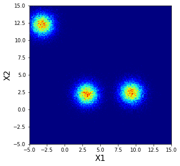
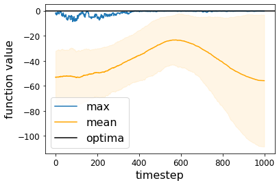
In particular, we sample a dataset $\mathcal{D}_{\text{GMM}}$ of size $5000$ points from a 3 component, equi-weighted Gaussian Mixture Model. The means are set as the three global maxima of $f_{br}$ and the covariance matrix for each component is identity (Figure 3(a)). We train DDOM with zero conditioning everywhere. As shown in Figure 3(b), DDOM can indeed approximate the GMM distribution. Consequently, with increasing timesteps, the denoised samples produced by the model get closer to the optima (Figure 3(c)).

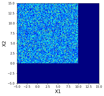
While the above experiment suggests that diffusion models can indeed be used for offline optimization, it makes an unrealistic assumption on the data distribution being concentrated around high function values by default. If we consider an alternate dataset $\mathcal{D}_{\text{Unif}}$ that is sampled uniformly from the domain (Figure 3(d)), DDOM learns to reproduce this uniform distribution (Figure 3(e)). In this case, the samples generated from the model become increasingly diverse with time, as evident from Figure 3(f).

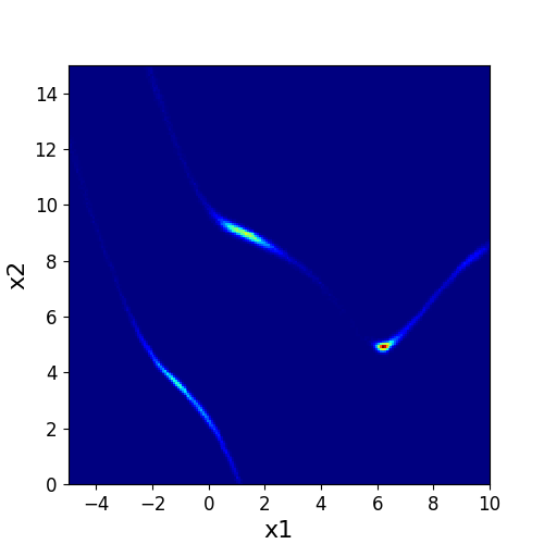
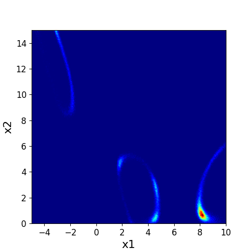
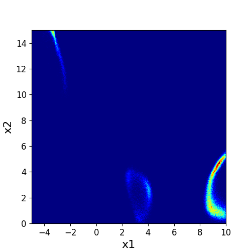
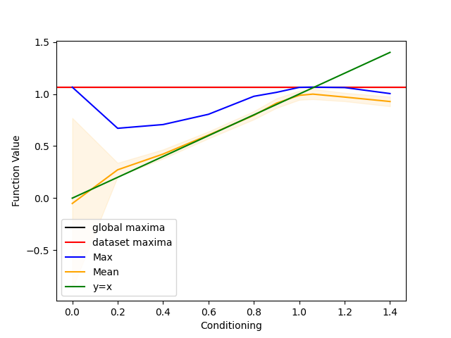
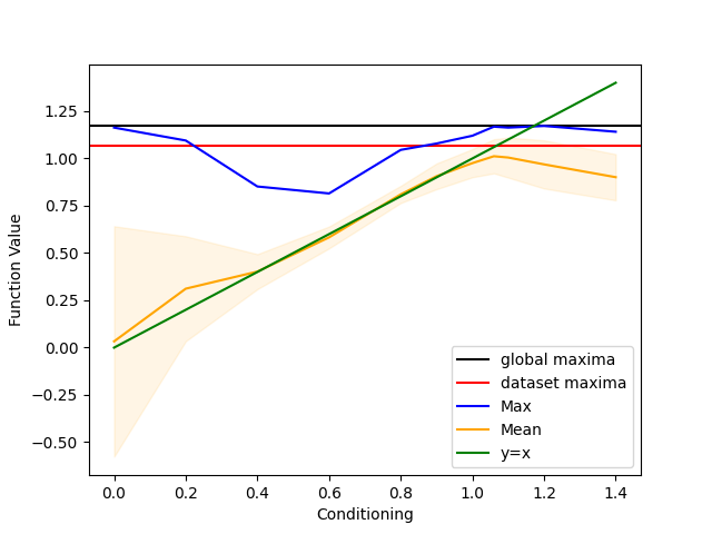
Conditional Diffusion Model With no control over the dataset quality, we need conditioning mechanisms, as described in Section 3. Consider the dataset $\mathcal{D}_{\text{Unif}}$ described above. We now train DDOM conditioned on $y$-values. In Figure 4, we can visualize the contours of the $f_{br}^{-1}(y)$ learned by our model for different conditioning values $y$. The top row shows the ground truth inverse contours calculated using a simple grid search. The bottom row is the histogram of $100,000$ samples from the last timestep of DDOM. We observe that the learned contours closely match the target contours for all conditioning values of $y$, suggesting an excellent learning of the one-to-many map $f_{br}^{-1}(y)$ in DDOM. We evaluate the performance of this model in terms of the mean and maximum function values of $256$ samples drawn from the final timestep of the diffusion model. Figure 5(a) shows that there is an expected increasing trend up to the conditioning equal to the dataset maxima, and then there is a slight dip. Furthermore, notice that the mean function value vs. conditioning curve is quite close to the $y=x$ line, showing that the model has learned the inverse well.

Generalization with Suboptimal Datasets The datasets we considered so far contain points close to the maxima. A key motivation for offline BBO is to generalize beyond the given dataset. To test this property for DDOM, we create a more challenging task by removing the top $10-\%$tile points from $\mathcal{D}_{\text{Unif}}$ based on their function values. We again train a conditional diffusion model and plot our predictions in Figure 5(b). We observe that the model is able to successfully propose points with function values higher than the dataset maximum. Further, the peak performance (in terms of both the best and mean function values) is when the conditioning is the maximum function value in the dataset.

4.2 Design-Bench

We also test DDOM on 6 high-dimensional real-world tasks in Design-Bench (Trabucco et al., 2022), a suite of offline BBO tasks. We test on three continuous and three discrete tasks. In D’Kitty and Ant Morphology, we need to optimize for the morphology of robots.In Superconductor (Supercond.), the aim is to optimize for finding a superconducting material with a high critical temperature.TFBind8 and TFBind10 are discrete tasks where the goal is to find a DNA sequence that has a maximum affinity to bind with a specified transcription factor. ChEMBL is a discrete task that optimizes drugs for specific chemical properties.

BASELINE	TFBIND8	TFBIND10	SUPERCON.	ANT	D’KITTY	CHEMBL	MEAN SCORE	MEAN RANK
$\mathcal{D}$ (best)	$0.439$	$0.467$	$0.399$	$0.565$	$0.884$	$0.605$	-	-
CbAS	$0.958\pm 0.018$	$0.657\pm 0.017$	$0.45\pm 0.083$	$0.876\pm 0.015$	$0.896\pm 0.016$	$0.640\pm 0.005$	$0.746\pm 0.003$	$5.5$
GP-qEI	$0.824\pm 0.086$	$0.635\pm 0.011$	$0.501\pm 0.021$	$0.887\pm 0.0$	$0.896\pm 0.0$	$0.633\pm 0.000$	$0.729\pm 0.019$	$6.2$
CMA-ES	$0.933\pm 0.035$	${\color[rgb]{.5,0,.5}\definecolor[named]{pgfstrokecolor}{rgb}{.5,0,.5}\mathbf{0.679\pm 0.034}}$	$0.491\pm 0.004$	${\color[rgb]{0,0,1}\definecolor[named]{pgfstrokecolor}{rgb}{0,0,1}\mathbf{1.436\pm 0.928}}$	$0.725\pm 0.002$	$0.636\pm 0.004$	${\color[rgb]{0,0,1}\definecolor[named]{pgfstrokecolor}{rgb}{0,0,1}\mathbf{0.816\pm 0.168}}$	$4.5$
Gradient Ascent	${\color[rgb]{0,0,1}\definecolor[named]{pgfstrokecolor}{rgb}{0,0,1}\mathbf{0.981\pm 0.015}}$	$0.659\pm 0.039$	${\color[rgb]{.5,0,.5}\definecolor[named]{pgfstrokecolor}{rgb}{.5,0,.5}\mathbf{0.504\pm 0.005}}$	$0.34\pm 0.034$	$0.906\pm 0.017$	$0.647\pm 0.020$	$0.672\pm 0.021$	${\color[rgb]{.5,0,.5}\definecolor[named]{pgfstrokecolor}{rgb}{.5,0,.5}\mathbf{3.5}}$
REINFORCE	$0.959\pm 0.013$	$0.64\pm 0.028$	$0.481\pm 0.017$	$0.261\pm 0.042$	$0.474\pm 0.202$	$0.636\pm 0.023$	$0.575\pm 0.054$	$6.3$
MINs	$0.938\pm 0.047$	$0.659\pm 0.044$	$0.484\pm 0.017$	$0.942\pm 0.018$	${\color[rgb]{.5,0,.5}\definecolor[named]{pgfstrokecolor}{rgb}{.5,0,.5}\mathbf{0.944\pm 0.009}}$	${\color[rgb]{0,0,1}\definecolor[named]{pgfstrokecolor}{rgb}{0,0,1}\mathbf{0.653\pm 0.002}}$	$0.770\pm 0.023$	${\color[rgb]{.5,0,.5}\definecolor[named]{pgfstrokecolor}{rgb}{.5,0,.5}\mathbf{3.5}}$
COMs	$0.964\pm 0.02$	$0.654\pm 0.02$	$0.423\pm 0.033$	$0.949\pm 0.021$	${\color[rgb]{0,0,1}\definecolor[named]{pgfstrokecolor}{rgb}{0,0,1}\mathbf{0.948\pm 0.006}}$	${\color[rgb]{.5,0,.5}\definecolor[named]{pgfstrokecolor}{rgb}{.5,0,.5}\mathbf{0.648\pm 0.005}}$	$0.764\pm 0.018$	$3.7$
DDOM	${\color[rgb]{.5,0,.5}\definecolor[named]{pgfstrokecolor}{rgb}{.5,0,.5}\mathbf{0.971\pm 0.005}}$	${\color[rgb]{0,0,1}\definecolor[named]{pgfstrokecolor}{rgb}{0,0,1}\mathbf{0.688\pm 0.092}}$	${\color[rgb]{0,0,1}\definecolor[named]{pgfstrokecolor}{rgb}{0,0,1}\mathbf{0.560\pm 0.044}}$	${\color[rgb]{.5,0,.5}\definecolor[named]{pgfstrokecolor}{rgb}{.5,0,.5}\mathbf{0.957\pm 0.012}}$	$0.926\pm 0.009$	$0.633\pm 0.007$	${\color[rgb]{.5,0,.5}\definecolor[named]{pgfstrokecolor}{rgb}{.5,0,.5}\mathbf{0.787\pm 0.034}}$	${\color[rgb]{0,0,1}\definecolor[named]{pgfstrokecolor}{rgb}{0,0,1}\mathbf{2.8}}$

Table 1: Comparative evaluation of DDOM over 6 tasks, with each task averaged over 5 seeds. We report normalized results (along with stddev) with a budget $Q=256$. We highlight the top two results in each column (and where there is a tie, we highlight both). ${\color[rgb]{0,0,1}\definecolor[named]{pgfstrokecolor}{rgb}{0,0,1}\mathbf{Blue}}$ refers to the best entry, and ${\color[rgb]{.5,0,.5}\definecolor[named]{pgfstrokecolor}{rgb}{.5,0,.5}\mathbf{Violet}}$ refers to the second best. We find that DDOM achieves the best average rank of all the baselines and is second best on the mean score metric.

	D’KITTY	ANT	TFBIND8	TFBIND10	SUPERCON.	CHEMBL
No reweighting	$0.926\pm 0.008$	$0.888\pm 0.018$	$0.957\pm 0.000$	$0.644\pm 0.011$	$0.553\pm 0.051$	$\mathbf{0.633\pm 0.000}$
Reweighting	$\mathbf{0.930\pm 0.003}$	$\mathbf{0.960\pm 0.015}$	$\mathbf{0.971\pm 0.005}$	$\mathbf{0.688\pm 0.092}$	$\mathbf{0.560\pm 0.044}$	$\mathbf{0.633\pm 0.000}$

Table 2: Comparison of normalized scores for DDOM with and without reweighting on Design-Bench. Higher is better We find that there is a significant improvement in score from reweighting on most tasks. We report scores averaged across 5 seeds.

Baselines We compare DDOM with multiple baselines using canonical approaches like gradient ascent, Bayesian Optimization (BayesOpt), REINFORCE (Sutton et al., 1999), evolutionary strategies like CMA-ES (Hansen, 2006), and newer methods like MINs (Kumar & Levine, 2020), COMs (Trabucco et al., 2021) and CbAS (Brookes et al., 2019). Since we are in the offline setting, for active methods like BayesOpt, we follow the procedure of Trabucco et al. (2022) and perform BayesOpt on a surrogate model $\hat{f}(\mathbf{x})$ trained on the offline dataset. We instantiate BayesOpt using a Gaussian Process as the uncertainty quantifier and the quasi-Expected Improvement (q-EI) acquisition function. For all tasks, we use a query budget $Q=256$. Following the procedure used by Trabucco et al. (2022), we report the results of all the tasks normalized using a larger unseen offline dataset, i.e. we report $y_{\texttt{norm}}$ where $y_{\texttt{norm}}=\frac{y-y_{\texttt{min}}}{y_{\texttt{max}}-y_{\texttt{min}}}$, where $y$, $y_{\texttt{min}}$ and $y_{\texttt{max}}$ refer to the score of the proposed solution, and the minimum and maximum of the large unseen offline dataset. Note that this larger dataset is not used for training but only for reporting normalized results. We also report the mean score and mean rank of all baselines.

Architecture We instantiate DDOM using a simple feed-forward neural network with 2 hidden layers, width of $1024$ and ReLU activation. We train using a fixed learning rate of $0.001$ and batch size of $128$. We set the minimum and maximum noise variance to be $0.01$ and $2.0$ respectively. We use the same value of $\gamma=2.0$ across all experiments.

Main Results In Table 1, we report normalized results of the max score achieved by DDOM and the baselines along with the mean normalized score and the mean rank. Overall we find that DDOM achieves an average rank of $2.8$, the best among all the baselines, and an average score of $0.787$. We achieve the best result on 2 tasks and are runner-up on another 2 tasks. On Superconductor, we outperform other baselines by a significant margin, beating the next closest baseline by 11%. We further note that CMA-ES, the baseline with the highest average score, has a standard deviation $5$ times as large as DDOM, indicating that it is very sensitive to initialization, unlike DDOM.

4.3 Ablations

We perform ablation studies on the different components of DDOM to study their effects: reweighting, conditioning, and classifier-free diffusion. We provide additional results and discussion in Appendix B.

Figure 6: Plot of mean function value versus conditioning for Superconductor. Dotted lines represent the dataset max and the line $y=x$ (the ideal line). Even for such a high-dimensional task, a strong correlation exists between predicted and conditioned values.

Figure 7: Change in mean objective values as a function of number of diffusion steps for multiple values of $\gamma$ for Superconductor. We find that when there is no guidance ($\gamma=0$), DDOM performs poorly, indicating the importance of guidance.

Reweighting We report results with and without reweighting in DDOM in Table 2 across 6 tasks. We find that across all tasks, the reweighted model outperforms the non-reweighted one, indicating the importance of reweighting.

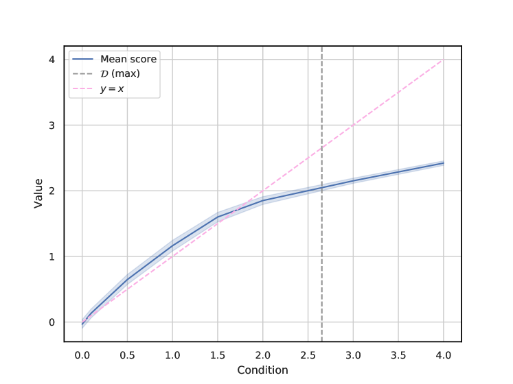
Impact of conditioning In Figure 6, we plot the mean of the predicted values against the conditioned value for the Superconductor task. We see that up to around the maxima of the dataset, both the conditioned and predicted values correlate very well with each other, suggesting that increasing the conditioning also increases the score of the predicted point. While generalizing beyond the dataset maxima is difficult when dealing with such a high-dimensional task, we notice a fairly high correlation between predicted and conditioned values even for very large conditioning values.

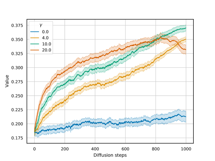
Impact of guidance We perform an ablation on the impact of the weighing factor in classifier-free guidance in Figure 7. We plot the average score of 512 samples from our model at various timesteps during the diffusion process for Superconductor. As expected, we find that no guidance $\gamma=0$ (i.e., a simple conditional diffusion model) performs very poorly compared to models with guidance, indicating the importance of classifier-free guidance. We also notice that increasing the guidance also increases the rate at which the predicted values increase, indicating the importance of using higher guidance weights during optimization.

5 Related Work

Active BBO Most prior work in BBO has been in the active setting, where models can query the function during training. Bayesian optimization is the most well-known active BBO method, and there is a large body of prior work in the area (Snoek et al., 2012; Shahriari et al., 2016; Srinivas et al., 2010; Zhang et al., 2022) inter alia. Such methods usually use surrogates like Gaussian Processes (GPs) to model the underlying function and sequentially update it by querying new points determined by an uncertainty-aware acquisition function. Bandit algorithms (Swaminathan & Joachims, 2015; Garivier et al., 2016; Grover et al., 2018; Joachims et al., 2018; Riquelme et al., 2018; Attia et al., 2020; Guo et al., 2021) are another well-known class of active BBO methods. DDOM is similar to Neural Diffusion Processes (NDP) (Dutordoir et al., 2022) in the use of diffusion processes for black-box optimization but operates in a purely offline setting, imposes no restrictions on the model architecture, and uses classifier-free guidance for generalization, unlike NDPs.

Offline BBO Recent works have shown significant progress in the offline setting (Trabucco et al., 2021; Kumar & Levine, 2020; Hansen, 2006; Fannjiang & Listgarten, 2020).  Trabucco et al. (2022) provides Design-Bench, a comprehensive real-world dataset for benchmarking offline BBO methods. Most methods (Trabucco et al., 2021, 2022; Nguyen & Grover, 2022) use forward models to approximate the black-box function and optimize it. On the other hand, methods like Kumar & Levine (2020) train generative models like GANs to model the one-to-many inverse mapping from function value to the input domain. CbAS (Brookes et al., 2019) learns a density model in the space of inputs that approximates the data distribution, and gradually adapts it towards an optimized solution. In particular CbAS alternates between training a VAE on a set of samples and generating new samples from the autoencoder which are then used to train the VAE on the next iteration.

Diffusion Models Diffusion models (Sohl-Dickstein et al., 2015) have recently shown strong performance in robust generative modeling for images (Song et al., 2020, 2021; Huang et al., 2021; Ho et al., 2020), videos (Ho et al., 2022), and audio (Kim et al., 2022; Jeong et al., 2021), as well as for planning in RL (Janner et al., 2022). The latter is particularly relevant and includes parallel advancements in the use of autoregressive and masked transformers that reduce sequential decision making to a generative modeling problem (Chen et al., 2021; Liu et al., 2022; Zhu et al., 2023; Nguyen et al., 2022; Zheng et al., 2022, 2023). Usually a model is trained to invert the forward diffusion process of converting data to noise sequentially by adding small Gaussian noise at each timestep. Our work can benefit from this growing area of research spanning advancements in conditioning and sampling strategies (Jolicoeur-Martineau et al., 2021; Karras et al., 2022; Bansal & Grover, 2023) and alternate diffusion parameterizations (Bansal et al., 2022; Hoogeboom & Salimans, 2022), among others.

6 Summary

We proposed Denoising Diffusion Optimization Models (DDOM), a new approach for offline black-box optimization based on conditional diffusion models. DDOM falls within the category of inverse approaches that train a mapping from function values to points. Unlike prior inverse approaches such as MINs (Kumar & Levine, 2020), DDOM is more stable to train and less susceptible to mode collapse. We noted two key modifications to the default setup: the use of loss reweighting to prioritize offline points with high function values and the use of classifier-guided sampling for improving the strength of conditioning at test time. Empirically, our approach is highly competitive and on average, outperforms both forward and inverse baselines on the Design-Bench suite (Trabucco et al., 2022).

Limitations and Future Work. Diffusion models is that they are relatively slow to sample compared to other generative approaches. While sampling speed is typically not a major bottleneck for offline BBO, it can be potentially limiting for some real-time applications. Given the fast-developing field of diffusion models for data generation, we expect many of the corresponding advancements in sampling and hyperparameter tuning (Karras et al., 2022) to transfer over to DDOM. Finally, we focused on offline BBO in this work. In some practical scenarios, we might also have resources for active data acquisition and future work can explore using DDOM to warm start a subsequent diffusion-based online BBO method.

Appendix A Notation and Experimental Details

A.1 Notation

SYMBOL	MEANING
$f$	Black box function
$\mathcal{X}$	Support of $f$
$\mathbf{x}^{*}$	Optima (taken to be maxima for consistency)
$\mathcal{D}$	Offline dataset
$Q$	Query budget for black-box function
$K,\tau$	Reweighting hyperparameters
$B_{i}$	Size of bin $i$

Table 3: Important notation used in our paper

A.2 Additional Experimental details

Code

We build on top of Huang et al. (2021) implementation of score based diffusion models (linked here). We provide our code via an anonymized link here. All code we use is under the MIT licence.

Training details

We train our model on one RTX A5000 GPU and report results averaged over 5 seeds. For all tasks in Design-Bench (Trabucco et al., 2022) we train with a batch size of $128$ for $1000$ epochs. For reweighting, we use a value of $K=0.01*N$ and $\tau=0.1$. For discrete tasks, we follow a similar procedure to Trabucco et al. (2022) and convert the $d$-to dimensional vector to a $c\times d$ size one hot vector. We then approximate logits by interpolating between a uniform distribution and the one hot distribution using a mixing factor of $0.6$. During training, we randomly set the conditioning value to 0 to jointly train a conditional and unconditional model with the same model. We use a dropout probability of 0.15, i.e. 15% of the time the conditioning value is set to zero

Evaluation

For all Design-bench tasks, we evaluate on a budget of $Q=256$ points. choice of the conditioning value is an important parameter for DDOM. As we see in Section 4.3, the predicted values increase upto around the dataset maxima before tapering off. This motivates us to use the dataset maxima for conditioning our model. Choosing the dataset maxima for conditioning has the advantages of being easy to implement for any type of dataset and not requiring any prior knowledge about the dataset (like the dataset maxima).

Design-Bench Tasks

We present additional information on the tasks we evaluate on in Design-Bench (Trabucco et al., 2022).

TASK	SIZE	DIMENSIONS	TASK MAX
TFBind8	32898	8	1.0
TFBind10	10000	10	2.128
ChEMBL	1093	31	443000.0
NAS	1771	64	69.63
D’Kitty	10004	56	340.0
Ant	10004	60	590.0
Superconductor	17014	86	185.0

Table 4: Dataset Statistics

A.3 Unnormalized results

We present the unnormalized results of Table 1 here, in Table 5.

BASELINE	TFBIND8	TFBIND10	SUPERCON.	ANT	D’KITTY	CHEMBL
$\mathcal{D}$ (best)	$0.439$	$0.00532$	$74.0$	$165.326$	$199.231$	$443000.000$
CbAS	$0.958\pm 0.018$	$0.761\pm 0.067$	$83.178\pm 15.372$	$468.711\pm 14.593$	$213.917\pm 19.863$	$389000.000\pm 500.000$
GP-qEI	$0.824\pm 0.086$	$0.675\pm 0.043$	${92.686\pm 3.944}$	$480.049\pm 0.000$	$213.816\pm 0.000$	$387950.000\pm 0.000$
CMA-ES	$0.933\pm 0.035$	${0.848\pm 0.136}$	$90.821\pm 0.661$	${1016.409\pm 906.407}$	$4.700\pm 2.230$	$388400.000\pm 400.000$
Gradient Ascent	${0.981\pm 0.010}$	$0.770\pm 0.154$	${93.252\pm 0.886}$	$-54.955\pm 33.482$	$226.491\pm 21.120$	$390050.000\pm 2000.000$
REINFORCE	$0.959\pm 0.013$	$0.692\pm 0.113$	$89.027\pm 3.093$	$-131.907\pm 41.003$	$-301.866\pm 246.284$	$388400.000\pm 2100.000$
MINs	$0.938\pm 0.047$	$0.770\pm 0.177$	$89.469\pm 3.227$	$533.636\pm 17.938$	$272.675\pm 11.069$	${390950.000\pm 200.000}$
COMs	$0.964\pm 0.020$	$0.750\pm 0.078$	$78.178\pm 6.179$	$540.603\pm 20.205$	${277.888\pm 7.799}$	$390200.000\pm 500.000$3
DDOM	$0.971\pm 0.005$	$0.885\pm 0.367$	$103.600\pm 8.139$	$548.227\pm 11.725$	$250.529\pm 10.992$	$387950.000\pm 1050.000$

Table 5: Unnormalized counterpart to results presented in Table 1

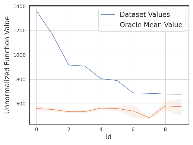
A.4 HopperController

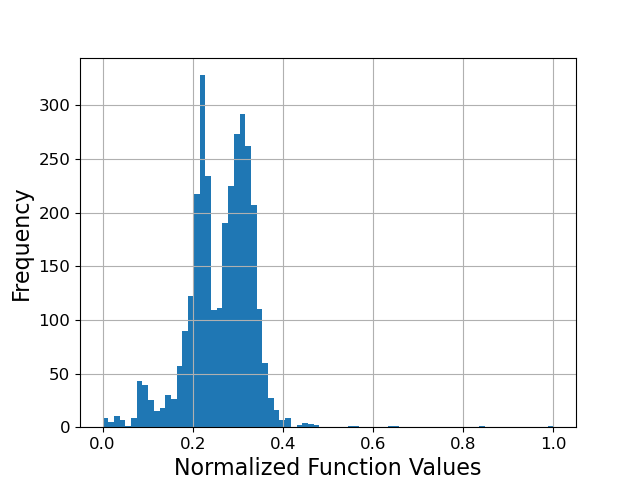
We don’t include the Hopper task in our results in Table 1 because of inconsistencies between the offline dataset values and the values obtained when running the oracle. A similar issue was noticed by Krishnamoorthy et al. (2023) in the Hopper task, and it seems to be a known bug in Design-bench (see here). Due to such discrepancies, we decided not to include Hopper in our analysis.

Figure 8: Histogram of normalized function values in the Hopper dataset. The distribution is highly skewed towards low function values. Plots taken from Krishnamoorthy et al. (2023)

Figure 9: Dataset values vs Oracle values for top $10$ points. Oracle being noisy, we show mean and standard deviation over $20$ runs. Plots taken from Krishnamoorthy et al. (2023).

Appendix B Additional Ablations and Analysis

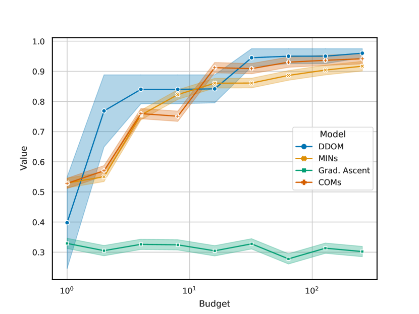
B.1 Effect of evaluation budget

In this experiment, we vary the evaluation budget $Q$ on Ant for DDOM to see how sensitive the quality of predictions are to the budget $Q$. The results are shown in Figure 10. We see that DDOM outperforms multiple baselines (namely MINs, COMs and Grad. Ascent) for various budget values, indicating that DDOM is consistently able to find good points.

Figure 10: Plot of maximum objective value versus budget $Q$ for Ant, averaged over 5 seeds. We find that DDOM outperforms MINs, COMs and Grad. Ascent on most choices of budget, indicating that DDOM is consistently able to find good points.

B.2 Ablation on reweighting parameters

During reweighting, we reweight the loss using the formula

$$w_{i}=\frac{|B_{i}|}{|B_{i}|+K}\exp{\left(\frac{-|\hat{y}-y_{b_{i}}|}{\tau}\right)}$$ (8)

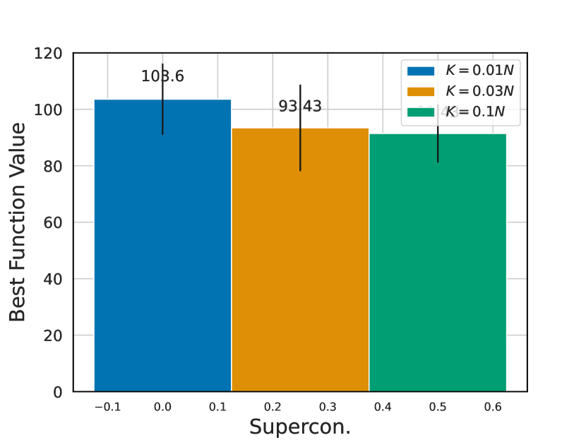
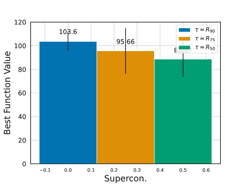
In the equation, $K$ and $\tau$ act as smoothing parameters. $\tau$ controls how much weight is given to good bins (bins with good points) versus bad bins. Lowering $\tau$ would lead to lower weights for low quality bins (bins with low scores) and vice versa. A smaller value of $K$ leads to bin size being an irrelevant factor in reweighting, meaning that weights are computed solely according to the values of the points. A large value of $K$ would lead to the reweighting scaling roughly linearly with the size of the bin.

In Figure 11 we plot the function value of superconductor achieved when using various values of $K$ and $\tau$.

Figure 11: Plot of function value of Superconductor for various values of $K$ and $\tau$

We further run an ablation on the number of bins on AntMorphology where we try out 3 different values of $N_{B}$. The results are in Table 6. We find that for 1 bin, we see a significant difference, in performance, but the difference is much smaller between 32 and 64 bins.

$N_{B}$	SCORE
$N_{B}=1$%	$480.820$
$N_{B}=32$%	$541.640$
$N_{B}=64$%	$548.227$

Table 6: Ablation on number of bins

B.3 Visualizing the Design-Bench datasets

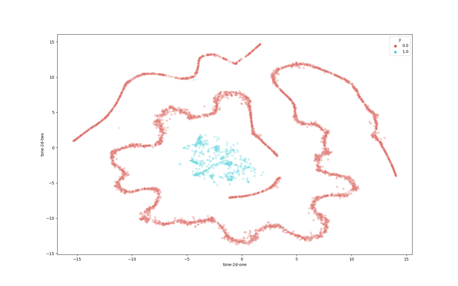
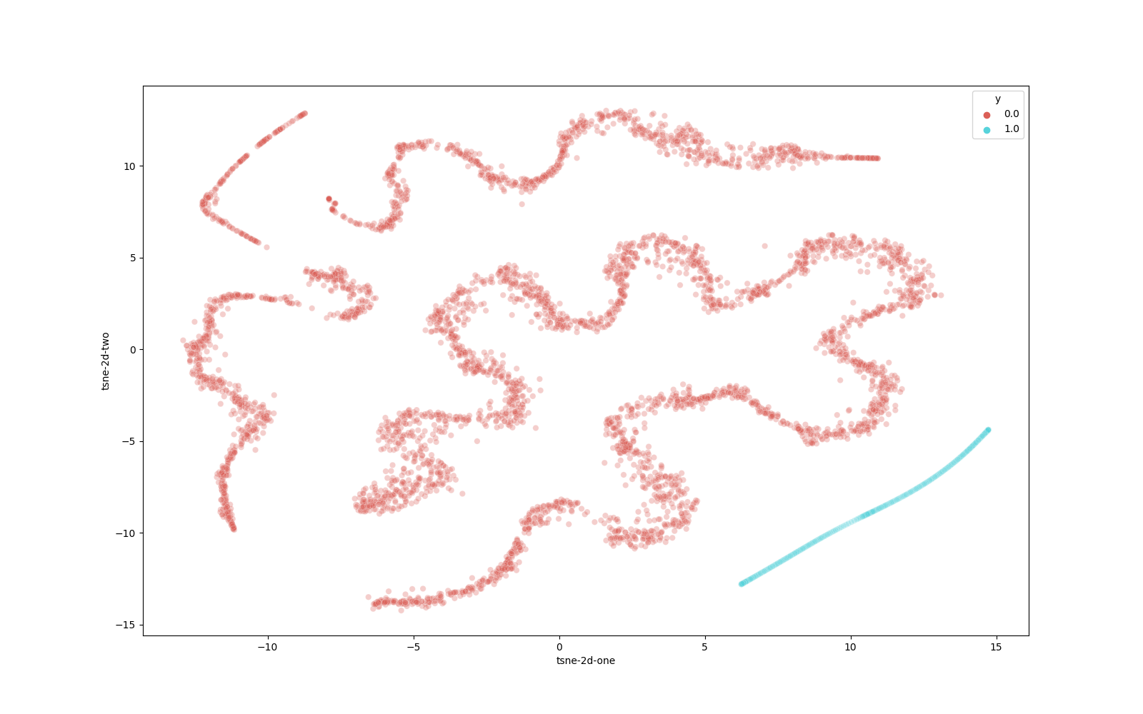
In Figure 12, we show plots of t-SNE of the dataset and predicted points for 3 continuous tasks, D’Kitty, Ant and Superconductor. The red points refer to dataset points, and the blue points refer to the points predicted by our model. We find that the points predicted by our model do not just follow the contours of the dataset points, indicating that the model is just not memorizing the dataset.

(a) Ant

(b) DKitty

(c) Superconductor

Figure 12: t-SNE plots of dataset and predicted points for D’Kitty, Ant and Superconductor. The red points refer to dataset points, and the blue points refer to the points predicted by our model. We find that the points predicted by our model do not just follow the contours of the dataset points, indicating that the model is just not memorizing the dataset

B.4 Plotting the contours of the score function

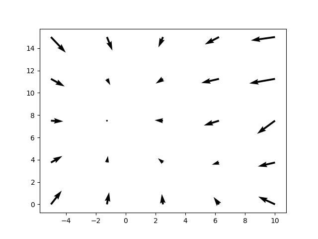
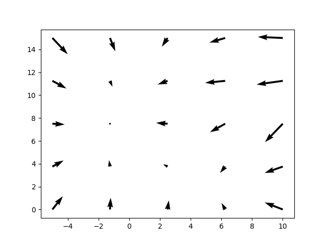
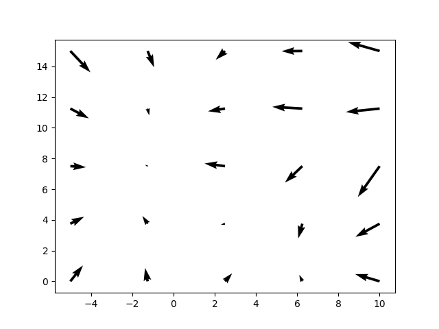
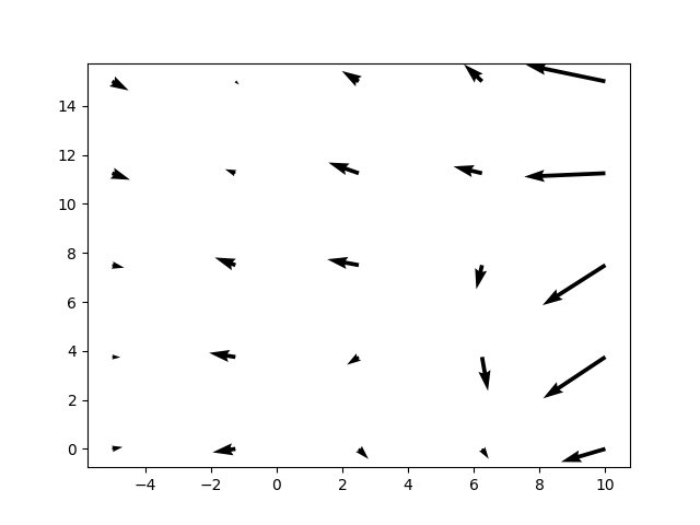
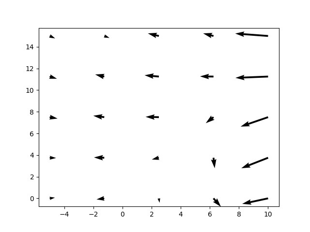
In Figure 13, we show the the contours of the score function on the Branin task across various timesteps. This illustrates how the learned score function varies with time.

(a) $t=0$

(b) $t=0.125$

(c) $t=0.25$

(d) $t=0.5$

(e) $t=0.875$

(f) $t=1.0$

Figure 13: In this plot, we show the the contours of the score function on the Branin task across various timesteps. This illustrates how the learned score function varies with time.

B.5 Effect of adding randomness to data

We run an experiment where we add noise to the function evaluations of Superconductor. The results are in Table 7. We find that with only a little noise, the performance isn’t affected too much. Even a significant fraction like 20% still sees only a moderate decline in performance.

NOISE (as a % of $\mathcal{D}$ (best))	SCORE
$0$%	$103.600$
$2$%	$98.470$
$20$%	$91.252$
$100$%	$79.374$

Table 7: Ablation on adding additional noise to data. Noise added is mentioned as a % of the dataset maxima

B.6 Effect of size of the offline dataset

We run an experiment on Superconductor where we randomly withhold some percentage of points from the offline dataset. The results are in Table 8 We find that even when removing parts of the offline dataset, the model is able to perform better than the dataset optima, indicating that there is a degree of generalizability.

% WITHHELD	SCORE
$10$%	$102.340$
$50$%	$97.200$
$90$%	$89.240$
$99$%	$83.120$

Table 8: Ablation on size of offline data

Appendix C Societal Impact

While we don’t anticipate anything to be inherently malicious about our work, it is possible that our method (and other optimizers like it) could be used in harmful settings (e.g. optimizing for drugs with adverse side effects). This is something to be careful of when deploying such optimizing algorithms in the real world.

References

- Attia et al. (2020) Attia, P., Grover, A., Jin, N., Severson, K., Cheong, B., Liao, J., Chen, M. H., Perkins, N., Yang, Z., Herring, P., Aykol, M., Harris, S., Braatz, R., Ermon, S., and Chueh, W. Closed-loop optimization of extreme fast charging for batteries using machine learning. Nature, 2020.
- Bansal et al. (2022) Bansal, A., Borgnia, E., Chu, H.-M., Li, J. S., Kazemi, H., Huang, F., Goldblum, M., Geiping, J., and Goldstein, T. Cold diffusion: Inverting arbitrary image transforms without noise. arXiv preprint arXiv:2208.09392, 2022.
- Bansal & Grover (2023) Bansal, H. and Grover, A. Leaving reality to imagination: Robust classification via generated datasets. arXiv preprint arXiv:2302.02503, 2023.
- Brookes et al. (2019) Brookes, D., Park, H., and Listgarten, J. Conditioning by adaptive sampling for robust design. In International Conference on Machine Learning, 2019.
- Chen et al. (2021) Chen, L., Lu, K., Rajeswaran, A., Lee, K., Grover, A., Laskin, M., Abbeel, P., Srinivas, A., and Mordatch, I. Decision transformer: Reinforcement learning via sequence modeling. arXiv preprint arXiv:2106.01345, 2021.
- Dhariwal & Nichol (2021) Dhariwal, P. and Nichol, A. Q. Diffusion models beat GANs on image synthesis. In Advances in Neural Information Processing Systems, 2021.
- Dutordoir et al. (2022) Dutordoir, V., Saul, A., Ghahramani, Z., and Simpson, F. Neural diffusion processes. arXiv preprint arXiv:2206.03992, 2022.
- Fannjiang & Listgarten (2020) Fannjiang, C. and Listgarten, J. Autofocused oracles for model-based design. In Advances in Neural Information Processing Systems, volume 33, 2020.
- Garivier et al. (2016) Garivier, A., Kaufmann, E., and Lattimore, T. On explore-then-commit strategies. In Proceedings of the 30th International Conference on Neural Information Processing Systems, 2016.
- Goodfellow et al. (2014) Goodfellow, I., Pouget-Abadie, J., Mirza, M., Xu, B., Warde-Farley, D., Ozair, S., Courville, A., and Bengio, Y. Generative adversarial nets. In Advances in Neural Information Processing Systems, 2014.
- Grover et al. (2018) Grover, A., Markov, T., Attia, P., Jin, N., Perkins, N., Cheong, B., Chen, M., Yang, Z., Harris, S., Chueh, W., and Ermon, S. Best arm identification in multi-armed bandits with delayed feedback. In International Conference on Artificial Intelligence and Statistics (AISTATS), 2018.
- Guo et al. (2021) Guo, W., Agrawal, K. K., Grover, A., Muthukumar, V., and Pananjady, A. Learning from an exploring demonstrator: Optimal reward estimation for bandits. In International Conference on Artificial Intelligence and Statistics (AISTATS), 2021.
- Hansen (2006) Hansen, N. The cma evolution strategy: a comparing review. Towards a new evolutionary computation: Advances in the estimation of distribution algorithms, pp. 75–102, 2006.
- Hansen (2016) Hansen, N. The cma evolution strategy: A tutorial. arXiv preprint arXiv:1604.00772, 2016.
- Ho & Salimans (2021) Ho, J. and Salimans, T. Classifier-free diffusion guidance. In NeurIPS 2021 Workshop on Deep Generative Models and Downstream Applications, 2021.
- Ho et al. (2020) Ho, J., Jain, A., and Abbeel, P. Denoising diffusion probabilistic models. In Advances in Neural Information Processing Systems, 2020.
- Ho et al. (2022) Ho, J., Salimans, T., Gritsenko, A. A., Chan, W., Norouzi, M., and Fleet, D. J. Video diffusion models. In Advances in Neural Information Processing Systems, 2022.
- Hoogeboom & Salimans (2022) Hoogeboom, E. and Salimans, T. Blurring diffusion models. arXiv preprint arXiv:2209.05557, 2022.
- Huang et al. (2021) Huang, C.-W., Lim, J. H., and Courville, A. C. A variational perspective on diffusion-based generative models and score matching. Advances in Neural Information Processing Systems, 34:22863–22876, 2021.
- Janner et al. (2022) Janner, M., Du, Y., Tenenbaum, J. B., and Levine, S. Planning with diffusion for flexible behavior synthesis. arXiv preprint arXiv:2205.09991, 2022.
- Jeong et al. (2021) Jeong, M., Kim, H., Cheon, S. J., Choi, B. J., and Kim, N. S. Diff-tts: A denoising diffusion model for text-to-speech. arXiv preprint arXiv:2104.01409, 2021.
- Joachims et al. (2018) Joachims, T., Swaminathan, A., and de Rijke, M. Deep learning with logged bandit feedback. In International Conference on Learning Representations, 2018.
- Jolicoeur-Martineau et al. (2021) Jolicoeur-Martineau, A., Li, K., Piché-Taillefer, R., Kachman, T., and Mitliagkas, I. Gotta go fast when generating data with score-based models. arXiv preprint arXiv:2105.14080, 2021.
- Karras et al. (2022) Karras, T., Aittala, M., Aila, T., and Laine, S. Elucidating the design space of diffusion-based generative models. arXiv preprint arXiv:2206.00364, 2022.
- Kim et al. (2022) Kim, H., Kim, S., and Yoon, S. Guided-tts: A diffusion model for text-to-speech via classifier guidance. In International Conference on Machine Learning. PMLR, 2022.
- Kong et al. (2021) Kong, Z., Ping, W., Huang, J., Zhao, K., and Catanzaro, B. Diffwave: A versatile diffusion model for audio synthesis. In International Conference on Learning Representations, 2021.
- Krishnamoorthy et al. (2023) Krishnamoorthy, S., Mashkaria, S. M., and Grover, A. Generative pretraining for black-box optimization. In International Conference on Machine Learning (ICML), 2023.
- Kumar & Levine (2020) Kumar, A. and Levine, S. Model inversion networks for model-based optimization. In Advances in Neural Information Processing Systems, 2020.
- Liu et al. (2022) Liu, F., Liu, H., Grover, A., and Abbeel, P. Masked autoencoding for scalable and generalizable decision making. In Advances in Neural Information Processing Systems (NeurIPS), 2022.
- Mirza & Osindero (2014) Mirza, M. and Osindero, S. Conditional generative adversarial nets. arXiv preprint arXiv:1411.1784, 2014.
- Nguyen & Grover (2022) Nguyen, T. and Grover, A. Transformer neural processes: Uncertainty-aware meta learning via sequence modeling. In International Conference on Machine Learning (ICML), 2022.
- Nguyen et al. (2022) Nguyen, T., Zheng, Q., and Grover, A. Reliable conditioning of behavioral cloning for offline reinforcement learning. arXiv preprint arXiv:2210.05158, 2022.
- Ramesh et al. (2021) Ramesh, A., Pavlov, M., Goh, G., Gray, S., Voss, C., Radford, A., Chen, M., and Sutskever, I. Zero-shot text-to-image generation. In International Conference on Machine Learning, 2021.
- Riquelme et al. (2018) Riquelme, C., Tucker, G., and Snoek, J. Deep bayesian bandits showdown: An empirical comparison of bayesian deep networks for thompson sampling. arXiv preprint arXiv:1802.09127, 2018.
- Saharia et al. (2022) Saharia, C., Chan, W., Saxena, S., Li, L., Whang, J., Denton, E. L., Ghasemipour, K., Gontijo Lopes, R., Karagol Ayan, B., Salimans, T., et al. Photorealistic text-to-image diffusion models with deep language understanding. Advances in Neural Information Processing Systems, 35:36479–36494, 2022.
- Shahriari et al. (2016) Shahriari, B., Swersky, K., Wang, Z., Adams, R. P., and de Freitas, N. Taking the human out of the loop: A review of bayesian optimization. Proceedings of the IEEE, 104(1):148–175, 2016. doi: 10.1109/JPROC.2015.2494218.
- Snoek et al. (2012) Snoek, J., Larochelle, H., and Adams, R. P. Practical bayesian optimization of machine learning algorithms. Neural information processing systems, 2012.
- Sohl-Dickstein et al. (2015) Sohl-Dickstein, J., Weiss, E. A., Maheswaranathan, N., and Ganguli, S. Deep unsupervised learning using nonequilibrium thermodynamics. In International Conference on Machine Learning, 2015.
- Song et al. (2020) Song, J., Meng, C., and Ermon, S. Denoising diffusion implicit models. arXiv preprint arXiv:2010.02502, 2020.
- Song et al. (2021) Song, Y., Sohl-Dickstein, J., Kingma, D. P., Kumar, A., Ermon, S., and Poole, B. Score-based generative modeling through stochastic differential equations. In International Conference on Learning Representations, 2021.
- Srinivas et al. (2010) Srinivas, N., Krause, A., Kakade, S., and Seeger, M. W. Gaussian Process Optimization in the Bandit Setting: No Regret and Experimental Design. In Proceedings of the 27th International Conference on Machine Learning, pp. 1015–1022. Omnipress, 2010.
- Sutton et al. (1999) Sutton, R. S., McAllester, D., Singh, S., and Mansour, Y. Policy gradient methods for reinforcement learning with function approximation. In Advances in Neural Information Processing Systems, 1999.
- Swaminathan & Joachims (2015) Swaminathan, A. and Joachims, T. Batch learning from logged bandit feedback through counterfactual risk minimization. Journal of Machine Learning Research, 16(52):1731–1755, 2015.
- Trabucco et al. (2021) Trabucco, B., Kumar, A., Geng, X., and Levine, S. Conservative objective models for effective offline model-based optimization. In International Conference on Machine Learning, 2021.
- Trabucco et al. (2022) Trabucco, B., Geng, X., Kumar, A., and Levine, S. Design-bench: Benchmarks for data-driven offline model-based optimization. In International Conference on Machine Learning, pp. 21658–21676. PMLR, 2022.
- Vincent (2011) Vincent, P. A connection between score matching and denoising autoencoders. Neural computation, 23(7):1661–1674, 2011.
- Zhang et al. (2022) Zhang, D., Fu, J., Bengio, Y., and Courville, A. Unifying likelihood-free inference with black-box sequence design and beyond. In International Conference on Learning Representations, 2022. URL https://openreview.net/forum?id=1HxTO6CTkz.
- Zheng et al. (2022) Zheng, Q., Zhang, A., and Grover, A. Online decision transformer. In International Conference on Machine Learning (ICML), pp. 27042–27059, 2022.
- Zheng et al. (2023) Zheng, Q., Henaff, M., Amos, B., and Grover, A. Semi-supervised offline reinforcement learning with action-free trajectories. In International Conference on Machine Learning (ICML), 2023.
- Zhu et al. (2023) Zhu, B., Dang, M., and Grover, A. Scaling pareto-efficient decision making via offline multi-objective rl. In International Conference on Learning Representations (ICLR), 2023.