Unbalanced Optimal Transport meets Sliced-Wasserstein

Abstract

Optimal transport (OT) has emerged as a powerful framework to compare probability measures, a fundamental task in many statistical and machine learning problems. Substantial advances have been made over the last decade in designing OT variants which are either computationally and statistically more efficient, or more robust to the measures/datasets to compare. Among them, sliced OT distances have been extensively used to mitigate optimal transport’s cubic algorithmic complexity and curse of dimensionality. In parallel, unbalanced OT was designed to allow comparisons of more general positive measures, while being more robust to outliers. In this paper, we propose to combine these two concepts, namely slicing and unbalanced OT, to develop a general framework for efficiently comparing positive measures. We propose two new loss functions based on the idea of slicing unbalanced OT, and study their induced topology and statistical properties. We then develop a fast Frank-Wolfe-type algorithm to compute these loss functions, and show that the resulting methodology is modular as it encompasses and extends prior related work. We finally conduct an empirical analysis of our loss functions and methodology on both synthetic and real datasets, to illustrate their relevance and applicability.

1 Introduction

Positive measures are ubiquitous in various fields, including data sciences and machine learning (ML) where they commonly serve as data representations. A common example is the density fitting task, which arises in generative modeling [1, 2]: the observed samples can be represented as a discrete positive measure $\alpha$ and the goal is to find a parametric measure $\beta_{\eta}$ which fits the best $\alpha$. This can be achieved by training a model that minimizes a loss function over $\eta$, usually defined as a distance between $\alpha$ and $\beta_{\eta}$. Therefore, it is important to choose a meaningful discrepancy with desirable statistical, robustness and computational properties. In particular, some settings require comparing arbitrary positive measures, i.e. measures whose total mass can have an arbitrary value, as opposed to probability distributions, whose total mass is equal to 1. In cell biology [3], for example, measures are used to represent and compare gene expressions of cell populations, and the total mass represents the population size.

(Unbalanced) Optimal Transport. Optimal transport has been chosen as a loss function in various ML applications. OT defines a distance between two positive measures of same mass $\alpha$ and $\beta$ (i.e. $m(\alpha)=m(\beta)$) by moving the mass of $\alpha$ toward the mass of $\beta$ with least possible effort. The mass equality can nevertheless be hindering by imposing a normalization of $\alpha$ and $\beta$ to enforce $m(\alpha)=m(\beta)$, which is potentially spurious and makes the problem less interpretable. In recent years, OT has then been extended to settings where measures have different masses, leading to the unbalanced OT (UOT) framework [4, 5, 6]. An appealing outcome of this new OT variant is its robustness to outliers which is achieved by discarding them before transporting $\alpha$ to $\beta$. UOT has been useful for many theoretical and practical applications, e.g. theory of deep learning [7, 8], biology [3, 9] and domain adaptation [10]. We refer to [11] for an extensive survey of UOT. Computing OT requires to solve a linear program whose complexity is cubical in the number $n$ of samples ($\mathcal{O}(n^{3}\log n)$). Besides, accurately estimating OT distances through empirical disributions is challenging as OT suffers from the curse of dimension [12]. A common workaround is to rely on OT variants with lower complexities and better statistical properties. Among the most popular, we can list entropic OT [13], minibatch OT [14] and sliced OT [15, 16]. In this paper, we will focus on the latter.

Slicing (U)OT and related work. Sliced OT leverages the OT 1D closed-form solution to define a new cost. It averages the OT cost between projections of $(\alpha,\beta)$ on 1D subspaces of $\mathbb{R}^{d}$. For 1D data, the OT solution can be computed through a sort algorithm, leading to an appealing $\mathcal{O}(n\operatorname{log}(n))$ complexity [17]. Furthermore, it has been shown to lift useful topological and statistical properties of OT from 1-dimensional to multi-dimensional settings [18, 19, 20]. It therefore helps to mitigate the curse of dimensionality making SOT-based algorithms theoretically-grounded, statistically efficient and efficiently solvable even on large-scale settings. These appealing properties motivated the development of several variants and generalizations, e.g. to different types or distributions of projections [21, 22, 23, 24] and non-Euclidean data [25, 26, 27]. The slicing operation has also been applied to partial OT [28, 29, 30], a particular case of UOT, in order to speed up comparisons of unnormalized measures at large scale. However, while (sliced) partial OT allows to compare measures with different masses, it assumes that each input measure is discrete and supported on points that all share the same mass (typically 1). In contrast, the Gaussian-Hellinger-Kantorovich (GHK) distance [4], another popular formulation of UOT, allows to compare measures with different masses and supported on points with varying masses, and has not been studied jointly with slicing.

Contributions. In this paper, we present the first general framework combining UOT and slicing. Our main contribution is the introduction of two novel sliced variants of UOT, respectively called Sliced UOT (SUOT) and Unbalanced Sliced OT (USOT). SUOT and USOT both leverage one-dimensional projections and the newly-proposed implementation of UOT in 1D [31], but differ in the penalization used to relax the constraint on the equality of masses: USOT essentially performs a global reweighting of the inputs measures $(\alpha,\beta)$, while SUOT reweights each projection of $(\alpha,\beta)$. Our work builds upon the Frank-Wolfe-type method [32] recently proposed in [31] to efficiently compute GHK between univariate measures, an instance of UOT which has not yet been combined with slicing. We derive the associated theoretical properties, along with the corresponding fast and GPU-friendly algorithms. We demonstrate its versatility and efficiency on challenging experiments, where slicing is considered on a non-Euclidean hyperbolic manifold, as a similarity measure for document classification, or for computing barycenters of geoclimatic data.

Outline. In Section 2, we provide background knowledge on UOT and sliced OT (SOT). In Section 3, we define our two new loss functions (SUOT and USOT) and prove their metric, topological, statistical and duality properties in wide generality. We then detail in Section 4 the numerical implementation of SUOT and USOT based on the Frank-Wolfe algorithm. We investigate their empirical performance on hyperbolic and geophysical data as well as document classification in Section 5.

2 Background

Unbalanced Optimal Transport. We denote by $\mathcal{M}_{+}(\mathbb{R}^{d})$ the set of all positive Radon measures on $\mathbb{R}^{d}$. For any $\alpha\in\mathcal{M}_{+}(\mathbb{R}^{d})$, $\mathrm{supp}(\alpha)$ is the support of $\alpha$ and $m(\alpha)=\int_{\mathbb{R}^{d}}\mathrm{d}\alpha(x)$ the mass of $\alpha$. We recall the standard formulation of unbalanced OT [4], which uses $\varphi$-divergences for regularization.

Definition 1.

(Unbalanced OT) Let $\alpha,\beta\in\mathcal{M}_{+}(\mathbb{R}^{d})$. Let $\varphi:\mathbb{R}\to\mathbb{R}\cup\{+\infty\}$ be an entropy function, i.e. $\varphi$ is convex, lower semicontinuous, $\text{{dom}}(\varphi)\triangleq\{x\in\mathbb{R},\,\varphi(x)<+\infty\}\subset[0,+\infty)$ and $\varphi(1)=0$. Denote $\varphi^{\prime}_{\infty}\triangleq\lim_{x\to+\infty}\varphi(x)/x$. The $\varphi$-divergence between $\alpha$ and $\beta$ is defined as,

$$\text{D}_{\varphi}(\alpha|\beta)\triangleq\int_{\mathbb{R}^{d}}\varphi\left(\frac{\mathrm{d}\alpha}{\mathrm{d}\beta}(x)\right)\mathrm{d}\beta(x)+\varphi^{\prime}_{\infty}\int_{\mathbb{R}^{d}}\mathrm{d}\alpha^{\bot}(x)\,,$$ (1)

where $\alpha^{\bot}$ is defined as $\alpha=(\mathrm{d}\alpha/\mathrm{d}\beta)\beta+\alpha^{\bot}$. Given two entropy functions $(\varphi_{1},\varphi_{2})$ and a cost $\text{{C}}_{d}:\mathbb{R}^{d}\times\mathbb{R}^{d}\to\mathbb{R}$, the unbalanced OT problem between $\alpha$ and $\beta$ reads

$$\text{{UOT}}(\alpha,\beta)\triangleq\inf_{\pi\in\mathcal{M}_{+}(\mathbb{R}^{d}\times\mathbb{R}^{d})}\int\text{{C}}_{d}(x,y)\mathrm{d}\pi(x,y)+\mathrm{D}_{\varphi_{1}}(\pi_{1}|\alpha)+\mathrm{D}_{\varphi_{2}}(\pi_{2}|\beta)\,,$$ (2)

where $(\pi_{1},\pi_{2})$ denote the marginal distributions of $\pi$.

When $\varphi_{1}=\varphi_{2}$ and $\varphi_{1}(x)=0$ for $x=1$, $\varphi_{1}(x)=+\infty$ otherwise, (2) boils down to the Kantorovich formulation of OT (or balanced OT), which we denote by $\text{{OT}}(\alpha,\beta)$. Indeed, in that case, $\mathrm{D}_{\varphi_{1}}(\pi_{1}|\alpha)=\mathrm{D}_{\varphi_{2}}(\pi_{2}|\beta)=0$ if $\pi_{1}=\alpha$ and $\pi_{2}=\beta$, $\mathrm{D}_{\varphi_{1}}(\pi_{1}|\alpha)=\mathrm{D}_{\varphi_{2}}(\pi_{2}|\beta)=+\infty$ otherwise.

Under suitable choices of entropy functions ($\varphi_{1},\varphi_{2})$, $\text{{UOT}}(\alpha,\beta)$ allows to compare $\alpha$ and $\beta$ even when $m(\alpha)\neq m(\beta)$ and can discard outliers, which makes it more robust than $\text{{OT}}(\alpha,\beta)$. Two common choices are $\varphi(x)=\rho\left|x-1\right|$ and $\varphi(x)=\rho(x\log(x)-x+1)$, where $\rho>0$ is a characteristic radius w.r.t. $\text{{C}}_{d}$. They respectively correspond to $\text{D}_{\varphi}=\rho\text{{TV}}$ (total variation distance [33]) and $\text{D}_{\varphi}=\rho\text{{KL}}$ (Kullback-Leibler divergence).

The UOT problem has been shown to admit an equivalent formulation obtained by deriving the dual of (2) and proving strong duality. Based on Proposition 1, computing $\text{{UOT}}(\alpha,\beta)$ consists in optimizing a pair of continuous functions $(f,g)$.

Proposition 1.

[4, Corollary 4.12] The UOT problem (2) can equivalently be written as

$$\text{{UOT}}(\alpha,\beta)=\sup_{f\oplus g\leq\text{{C}}_{d}}\int\varphi^{\circ}_{1}(f(x))\mathrm{d}\alpha(x)+\int\varphi^{\circ}_{2}(g(y))\mathrm{d}\beta(y),$$ (3)

where for $i\in\{1,2\}$, $\varphi_{i}^{\circ}(x)\triangleq-\varphi_{i}^{*}(-x)$ with $\varphi_{i}^{*}(x)\triangleq\sup_{y\geq 0}xy-\varphi_{i}(y)$ the Legendre transform of $\varphi_{i}$, and $f\oplus g\leq\text{{C}}_{d}$ means that for $(x,y)\sim\alpha\otimes\beta$, $f(x)+g(y)\leq\text{{C}}_{d}(x,y)$.

In this paper, we mainly focus on the GHK setting, both theoretically and computationally. It corresponds to (2) with $\text{{C}}_{d}(x,y)=||x-y||^{2}$, $\text{D}_{\varphi_{i}}=\rho_{i}\text{{KL}}$, leading to $\varphi_{i}^{\circ}(x)=\rho_{i}(1-e^{-x/\rho_{i}})$. $\text{{UOT}}(\alpha,\beta)$ is known to be computationally intensive [34], thus motivating the development of methods that can scale to dimensions and sample sizes encountered in ML applications.

Sliced Optimal Transport. Among the many workarounds that have been proposed to overcome the OT computational bottleneck [17], Sliced OT [35] has attracted a lot of attention due to its computational benefits and theoretical guarantees. We define it below.

Definition 2 (Sliced OT).

Let $\mathbb{S}^{d-1}\triangleq\{\theta\in\mathbb{R}^{d}~{}:~{}\|\theta\|=1\}$ be the unit sphere in $\mathbb{R}^{d}$. For $\theta\in\mathbb{S}^{d-1}$, denote by $\theta^{\star}:\mathbb{R}^{d}\to\mathbb{R}$ the linear map such that for $x\in\mathbb{R}^{d}$, $\theta^{\star}(x)\triangleq\left\langle\theta,x\right\rangle$. Let $\bm{\sigma}$ be the uniform probability over $\mathbb{S}^{d-1}$. Consider $\alpha,\beta\in\mathcal{M}_{+}(\mathbb{R}^{d})$. The Sliced OT problem is defined as

$$\text{{SOT}}(\alpha,\beta)\triangleq\int_{\mathbb{S}^{d-1}}\text{{OT}}(\theta^{\star}_{\sharp}\alpha,\theta^{\star}_{\sharp}\beta)\mathrm{d}\bm{\sigma}(\theta)\,,$$ (4)

where for any measurable function $f$ and $\xi\in\mathcal{M}_{+}(\mathbb{R}^{d})$, $f_{\sharp}\xi$ is the push-forward measure of $\xi$ by $f$, i.e. for any measurable set $\textsc{A}\subset\mathbb{R}$, $f_{\sharp}\xi(\textsc{A})\triangleq\xi(f^{-1}(\textsc{A}))$, $f^{-1}(\textsc{A})\triangleq\{x\in\mathbb{R}^{d}:f(x)\in\textsc{A}\}$.

Note that $\theta^{\star}_{\sharp}\alpha,\theta^{\star}_{\sharp}\beta$ are two measures supported on $\mathbb{R}$, therefore $\text{{OT}}(\theta^{\star}_{\sharp}\mu,\theta^{\star}_{\sharp}\nu)$ is defined in terms of a cost function $\text{{C}}_{1}:\mathbb{R}\times\mathbb{R}\rightarrow\mathbb{R}$. Since OT between univariate measures can be efficiently computed, $\text{{SOT}}(\alpha,\beta)$ can provide significant computational advantages over $\text{{OT}}(\alpha,\beta)$ in large-scale settings. In practice, if $\alpha$ and $\beta$ are discrete measures supported on $\{x_{i}\}_{i=1}^{n}$ and $\{y_{i}\}_{i=1}^{n}$ respectively, the standard procedure for approximating $\text{{SOT}}(\alpha,\beta)$ consists in (i) sampling $m$ i.i.d. samples $\{\theta_{j}\}_{j=1}^{m}$ from $\bm{\sigma}$, (ii) computing $\text{{OT}}((\theta_{j}^{\star})_{\sharp}\alpha,(\theta_{j}^{\star})_{\sharp}\beta)$, $j=1,\dots,m$. Computing OT between univariate discrete measures amounts to sorting [17, Section 2.6], thus step (ii) involves $\mathcal{O}(n\log n)$ operations for each $\theta_{j}$.

$\text{{SOT}}(\alpha,\beta)$ is defined in terms of the Kantorovich formulation of OT, hence inherits the following drawbacks: $\text{{SOT}}(\alpha,\beta)<+\infty$ only when $m(\alpha)=m(\beta)$, and may not provide meaningful comparisons in presence of outliers. To overcome such limitations, prior work have proposed sliced versions of partial OT [28, 29], a particular instance of UOT. However, their contributions only apply to measures whose samples have constant mass. In the next section, we generalize their line of work and propose a new way of combining sliced OT and unbalanced OT.

3 Sliced Unbalanced OT and Unbalanced Sliced OT: Theoretical Analysis

We propose two strategies to make unbalanced OT scalable, by leveraging sliced OT. We formulate two loss functions (Definition 3), then study their theoretical properties and discuss their implications.

Definition 3.

Let $\alpha,\beta\in\mathcal{M}_{+}(\mathbb{R}^{d})$. The Sliced Unbalanced OT loss (SUOT) and the Unbalanced Sliced OT loss (USOT) between $\alpha$ and $\beta$ are defined as,

$$\text{{SUOT}}(\alpha,\beta) \triangleq\int_{\mathbb{S}^{d-1}}\text{{UOT}}(\theta^{\star}_{\sharp}\alpha,\theta^{\star}_{\sharp}\beta)\mathrm{d}\bm{\sigma}(\theta)\,,$$ (5)

$$\text{{USOT}}(\alpha,\beta) \triangleq\inf_{(\pi_{1},\pi_{2})\in\mathcal{M}_{+}(\mathbb{R}^{d})\times\mathcal{M}_{+}(\mathbb{R}^{d})}\text{{SOT}}(\pi_{1},\pi_{2})+\mathrm{D}_{\varphi_{1}}(\pi_{1}|\alpha)+\mathrm{D}_{\varphi_{2}}(\pi_{2}|\beta)\,.$$ (6)

$\text{{SUOT}}(\alpha,\beta)$ compares $\alpha$ and $\beta$ by solving the UOT problem between $\theta^{\star}_{\sharp}\alpha$ and $\theta^{\star}_{\sharp}\beta$ for $\theta\sim\bm{\sigma}$. Note that SUOT extends the sliced partial OT problem [28, 29] (where $\text{D}_{\varphi_{i}}=\rho_{i}\text{{TV}}$) by allowing the use of arbitrary $\varphi$-divergences. On the other hand, USOT is a completely novel approach and stems from the following property on UOT [4, Equations (4.21)]: $\text{{UOT}}(\alpha,\beta)=\inf_{(\pi_{1},\pi_{2})\in\mathcal{M}_{+}(\mathbb{R}^{d})^{2}}\text{{OT}}(\pi_{1},\pi_{2})+\mathrm{D}_{\varphi_{1}}(\pi_{1}|\alpha)+\mathrm{D}_{\varphi_{2}}(\pi_{2}|\beta)$.

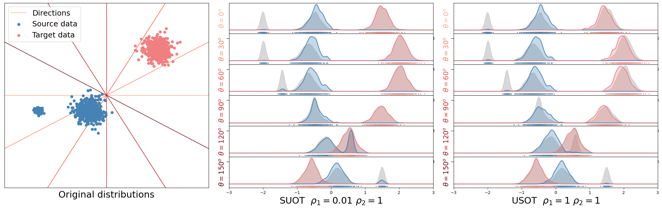
Figure 1: Toy illustration on the behaviors of SUOT and USOT. (left) Original 2D samples and slices used for illustration. KDE density estimations of the projected samples: grey, original distributions, colored, distributions reweighed by SUOT (center), and reweighed by USOT (right).

SUOT vs. USOT. As outlined in Definition 3, SUOT and USOT differ in how the transportation problem is penalized: $\text{{SUOT}}(\alpha,\beta)$ regularizes the marginals of $\pi_{\theta}$ for $\theta\sim\bm{\sigma}$ where $\pi_{\theta}$ denotes the solution of $\text{{UOT}}(\theta^{\star}_{\sharp}\alpha,\theta^{\star}_{\sharp}\beta)$, while $\text{{USOT}}(\alpha,\beta)$ operates a geometric normalization directly on $(\alpha,\beta)$. We illustrate this difference on the following practical setting: we consider $(\alpha,\beta)\in\mathcal{M}_{+}(\mathbb{R}^{2})$ where $\alpha$ is polluted with some outliers, and we compute $\text{{SUOT}}(\alpha,\beta)$ and $\text{{USOT}}(\alpha,\beta)$. We plot the input measures and the sampled projections $\{\theta_{k}\}_{k}$ (Figure 1, left), the marginals of $\pi_{\theta_{k}}$ for SUOT and the marginals of $(\theta_{k})_{\sharp}^{\star}\pi$ for USOT (Figure 1, right). As expected, SUOT marginals change for each $\theta_{k}$. We also observe that the source outliers have successfully been removed for any $\theta$ when using USOT, while they may still appear with SUOT (e.g. for $\theta=120^{\circ}$): this is a direct consequence of the penalization terms $\text{D}_{\varphi_{i}}$ in USOT, which operate on $(\alpha,\beta)$ rather than on their projections.

Theoretical analysis. In the rest of this section, we prove a set of theoretical properties of SUOT and USOT. All proofs are provided in Appendix A. We first identify the conditions on the cost $\text{{C}}_{1}$ and entropies $\varphi_{1},\varphi_{2}$ under which the infimum is attained in $\text{{UOT}}(\theta^{\star}_{\sharp}\alpha,\theta^{\star}_{\sharp}\beta)$ for $\theta\in\mathbb{S}^{d-1}$ and in $\text{{USOT}}(\alpha,\beta)$: the formal statement is given in Appendix A. We also show that these optimization problems are convex, both SUOT and USOT are jointly convex w.r.t. their input measures, and that strong duality holds (Theorem 5).

Next, we prove that both SUOT and USOT preserve some topological properties of UOT, starting with the metric axioms as stated in the next proposition.

Proposition 2.

(Metric properties) (i) Suppose UOT is non-negative, symmetric and/or definite on $\mathcal{M}_{+}(\mathbb{R})\times\mathcal{M}_{+}(\mathbb{R})$. Then, SUOT is respectively non-negative, symmetric and/or definite on $\mathcal{M}_{+}(\mathbb{R}^{d})\times\mathcal{M}_{+}(\mathbb{R}^{d})$. If there exists $p\in[1,+\infty)$ s.t. for any $(\alpha,\beta,\gamma)\in\mathcal{M}_{+}(\mathbb{R})$, $\text{{UOT}}^{1/p}(\alpha,\beta)\leq\text{{UOT}}^{1/p}(\alpha,\gamma)+\text{{UOT}}^{1/p}(\gamma,\beta)$, then $\text{{SUOT}}^{1/p}(\alpha,\beta)\leq\text{{SUOT}}^{1/p}(\alpha,\gamma)+\text{{SUOT}}^{1/p}(\gamma,\beta)$.

(ii) For any $\alpha,\beta\in\mathcal{M}_{+}(\mathbb{R}^{d})$, $\text{{USOT}}(\alpha,\beta)\geq 0$. If $\varphi_{1}=\varphi_{2}$, USOT is symmetric. If $\text{D}_{\varphi_{1}}$ and $\text{D}_{\varphi_{2}}$ are definite, then USOT is definite.

By Proposition 2(i), establishing the metric axioms of UOT between univariate measures (e.g., as detailed in [11, Section 3.3.1]) suffices to prove the metric axioms of SUOT between multivariate measures. Since e.g. GHK [4, Theorem 7.25] is a metric for $p=2$, then so is the associated SUOT.

In our next theorem, we show that SUOT, USOT and UOT are equivalent, under certain assumptions on the entropies $(\varphi_{1},\varphi_{2})$, cost functions, and input measures $(\alpha,\beta)$.

Theorem 1.

(Equivalence of $\text{{SUOT}},\text{{USOT}},\text{{UOT}}$) Let $\mathsf{X}$ be a compact subset of $\mathbb{R}^{d}$ with radius $R$. Let $p\in[1,+\infty)$ and assume $\text{{C}}_{1}(x,y)=\left|x-y\right|^{p}$, $\text{{C}}_{d}(x,y)=\|x-y\|^{p}$. Consider that $D_{\varphi_{1}}=D_{\varphi_{2}}=\rho\text{{KL}}$. Then, for any $\alpha,\beta\in\mathcal{M}_{+}(\mathsf{X})$,

$$\text{{SUOT}}(\alpha,\beta)\leq\text{{USOT}}(\alpha,\beta)\leq\text{{UOT}}(\alpha,\beta)\leq c(m(\alpha),m(\beta),\rho,R)\text{{SUOT}}(\alpha,\beta)^{1/(d+1)}\,,$$ (7)

where $c(m(\alpha),m(\beta),\rho,R)$ is constant depending on $m(\alpha),m(\beta),\rho,R$, which is non-decreasing in $m(\alpha)$ and $m(\beta)$. Additionally, assume there exists $M>0$ s.t. $m(\alpha)\leq M,m(\beta)\leq M$. Then, $c(m(\alpha),m(\beta),\rho,R)$ no longer depends on $m(\alpha),m(\beta)$, which proves the equivalence of SUOT, USOT and UOT.

Theorem 1 is an application of a more general result, which we derive in the appendix. In particular, we show that the first two inequalities in (7) hold under milder assumptions on $\varphi_{1},\varphi_{2}$ and $\text{{C}}_{1},\text{{C}}_{d}$. The equivalence of $\text{{SUOT}},\text{{USOT}}$ and UOT is useful to prove that SUOT and USOT metrize the weak^∗ convergence when UOT does, e.g. in the GHK setting [4, Theorem 7.25]. Before formally stating this result, we recall that a sequence of positive measures $(\alpha_{n})_{n\in\mathbb{N}^{*}}$ converges weakly to $\alpha\in\mathcal{M}_{+}(\mathbb{R}^{d})$ (denoted $\alpha_{n}\rightharpoonup\alpha$) if for any continuous $f:\mathbb{R}^{d}\rightarrow\mathbb{R}$, $\lim_{n\to+\infty}\int f\mathrm{d}\alpha_{n}=\int f\mathrm{d}\alpha$.

Theorem 2.

(Weak^∗ metrization) Assume $\text{D}_{\varphi_{1}}=\text{D}_{\varphi_{2}}=\rho\text{{KL}}$. Let $p\in[1,+\infty)$ and consider $\text{{C}}_{1}(x,y)=\left|x-y\right|^{p}$, $\text{{C}}_{d}(x,y)=\|x-y\|^{p}$. Let $(\alpha_{n})$ be a sequence of measures in $\mathcal{M}_{+}(\mathsf{X})$ and $\alpha\in\mathcal{M}_{+}(\mathsf{X})$, where $\mathsf{X}\subset\mathbb{R}^{d}$ is compact with radius $R>0$. Then, SUOT and USOT metrizes the weak^∗ convergence, i.e.

$$\alpha_{n}\rightharpoonup\alpha\Leftrightarrow\lim_{n\to+\infty}\text{{SUOT}}(\alpha_{n},\alpha)=0\Leftrightarrow\lim_{n\to+\infty}\text{{USOT}}(\alpha_{n},\alpha)=0.$$

The metrization of weak^∗ convergence is an important property when comparing measures. For instance, it can be leveraged to justify the well-posedness of approximating an unbalanced Wasserstein gradient flow [36] using SUOT, as done in [37, 38] for SOT. Unbalanced Wasserstein gradient flows have been a key tool in deep learning theory, e.g. to prove global convergence of 1-hidden layer neural networks [7, 8].

We now specialize some metric and topological properties to sliced partial OT, a particular case of SUOT. Theorem 3 shows that our framework encompasses existing approaches and more importantly, helps complement their analysis [28, 29].

Theorem 3.

(Properties of Sliced Partial OT) Assume $\text{{C}}_{1}(x,y)=\left|x-y\right|$ and $\text{D}_{\varphi_{1}}=\text{D}_{\varphi_{2}}=\rho\text{{TV}}$. Then, USOT satisfies the triangle inequality. Additionally, for any $(\alpha,\beta)\in\mathcal{M}_{+}(\mathsf{X})$ where $\mathsf{X}\subset\mathbb{R}^{d}$ is compact with radius $R$, $\text{{UOT}}(\alpha,\beta)\leq c(\rho,R)\,\text{{SUOT}}(\alpha,\beta)^{1/(d+1)}$, and USOT and SUOT both metrize the weak^∗ convergence.

We move on to the statistical properties and prove that SUOT offers important statistical benefits, as it lifts the sample complexity of UOT from one-dimensional setting to multi-dimensional ones. In what follows, for any $\alpha\in\mathcal{M}_{+}(\mathbb{R}^{d})$, we use $\hat{\alpha}_{n}$ to denote the empirical approximation of $\alpha$ over $n\geq 1$ i.i.d. samples, i.e. $\hat{\alpha}_{n}=\frac{1}{n}\sum_{i=1}^{n}\updelta_{Z_{i}}$, $Z_{i}\sim\alpha$ for $i=1,\dots,n$.

Theorem 4.

(Sample complexity) (i) If for $(\mu,\nu)\in\mathcal{M}_{+}(\mathbb{R})$, $\mathbb{E}|\text{{UOT}}(\mu,\nu)-\text{{UOT}}(\hat{\mu}_{n},\hat{\nu}_{n})|\leq\kappa(n)$, then for $(\alpha,\beta)\in\mathcal{M}_{+}(\mathbb{R}^{d})$, $\mathbb{E}|\text{{SUOT}}(\alpha,\beta)-\text{{SUOT}}(\hat{\alpha}_{n},\hat{\beta}_{n})|\leq\kappa(n)$.

(ii) If for $(\mu,\nu)\in\mathcal{M}_{+}(\mathbb{R})$, $\mathbb{E}|\text{{UOT}}(\mu,\hat{\mu}_{n})|\leq\xi(n)$, then for $(\alpha,\beta)\in\mathcal{M}_{+}(\mathbb{R}^{d})$, $\mathbb{E}|\text{{SUOT}}(\alpha,\hat{\alpha}_{n})|\leq\xi(n)$.

Theorem 4 means that SUOT enjoys a dimension-free sample complexity, even when comparing multivariate measures: this advantage is recurrent of sliced divergences [19] and further motivates their use on high-dimensional settings. The sample complexity rates $\kappa(n)$ or $\xi(n)$ can be deduced from the literature on UOT for univariate measures, for example we refer to [39] for the GHK setting. Establishing the statistical properties of USOT may require extending the analysis in [40]: we leave this question for future work.

We conclude this section by deriving the dual formulations of $\text{{SUOT}},\text{{USOT}}$ and proving that strong duality holds. We will consider that $\bm{\sigma}$ is approximated with $\hat{\bm{\sigma}}_{K}=\frac{1}{K}\sum_{k=1}^{K}\updelta_{\theta_{k}}$, $\theta_{k}\sim\bm{\sigma}$. This corresponds to the routine case in practice, as practitioners usually resort to a Monte Carlo approximation to estimate the expectation w.r.t. $\bm{\sigma}$ defining sliced OT.

Theorem 5.

(Strong duality) For $i\in\{1,2\}$, let $\varphi_{i}$ be an entropy function s.t. $\text{{dom}}(\varphi_{i}^{*})\cap\mathbb{R}_{-}$ is non-empty, and either $0\in\text{{dom}}(\varphi_{i})$ or $m(\alpha),m(\beta)\in\text{{dom}}(\varphi_{i})$. Define $\mathcal{E}\triangleq\{\forall\theta\in\mathrm{supp}(\sigma_{K}),\,f_{\theta}\oplus g_{\theta}\leq\text{{C}}_{1}\}$. Let $f_{avg}\triangleq\int_{\mathbb{S}^{d-1}}f_{\theta}\mathrm{d}\hat{\bm{\sigma}}_{K}(\theta)$, $g_{avg}\triangleq\int_{\mathbb{S}^{d-1}}g_{\theta}\mathrm{d}\hat{\bm{\sigma}}_{K}(\theta)$.

Then, SUOT (5) and USOT (6) can be equivalently written for $\alpha,\beta\in\mathcal{M}_{+}(\mathbb{R}^{d})$ as,

$$\text{{SUOT}}(\alpha,\beta) =\sup_{(f_{\theta}),(g_{\theta})\in\mathcal{E}}\int_{\mathbb{S}^{d-1}}\Big{(}\int\varphi_{1}^{\circ}\big{(}f_{\theta}\circ\theta^{\star}(x)\big{)}\mathrm{d}\alpha(x)+\int\varphi_{2}^{\circ}\big{(}g_{\theta}\circ\theta^{\star}(y)\big{)}\mathrm{d}\beta(y)\Big{)}\mathrm{d}\hat{\bm{\sigma}}_{K}(\theta)$$ (8)

$$\text{{USOT}}(\alpha,\beta) =\sup_{(f_{\theta}),(g_{\theta})\in\mathcal{E}}\int\varphi_{1}^{\circ}\big{(}f_{avg}\circ\theta^{\star}(x)\big{)}\mathrm{d}\alpha(x)+\int\varphi_{2}^{\circ}\big{(}g_{avg}\circ\theta^{\star}(y)\big{)}\mathrm{d}\beta(y)$$ (9)

We conjecture that strong duality also holds for $\bm{\sigma}$ Lebesgue over $\mathbb{S}^{d-1}$, and discuss this aspect in Appendix A. Theorem 5 has important pratical implications, since it justifies the Frank-Wolfe-type algorithms that we develop in Section 4 to compute SUOT and USOT in practice.

4 Computing SUOT and USOT with Frank-Wolfe algorithms

In this section, we explain how to implement SUOT and USOT. We propose two algorithms by leveraging our strong duality result (Theorem 5) along with a Frank-Wolfe algorithm (FW, [32]) introduced in [31] to optimize UOT dual 3. Our methods, summarized in Algorithms 1 and 2, can be applied for smooth $\text{D}_{\varphi_{1}},\text{D}_{\varphi_{2}}$: this condition is satisfied in the GHK setting (where $\text{D}_{\varphi_{i}}=\rho_{i}\text{{KL}}$), but not for sliced partial OT (where $\text{D}_{\varphi_{i}}=\rho_{i}\text{{TV}}$, [29]). We refer to Appendix B for more details on the technical implementation and theoretical justification of our methodology.

FW is an iterative procedure which aims at maximizes a functional $\mathcal{H}$ over a compact convex set $\mathcal{E}$, by maximizing a linear approximation $\nabla\mathcal{H}$: given iterate $x^{t}$, FW solves the linear oracle $r^{t+1}\in\arg\max_{r\in\mathcal{E}}\left\langle\nabla\mathcal{H}(x^{t}),r\right\rangle$ and performs a convex update $x^{t+1}=(1-\gamma_{t+1})x^{t}+\gamma_{t+1}r^{t+1}$, with $\gamma_{t+1}$ typically chosen as $\gamma_{t+1}=2/(2+t+1)$. We call this step FWStep in our pseudo-code. When applied in [31] to compute $\text{{UOT}}(\alpha,\beta)$ dual (3), FWStep updates $(f_{t},g_{t})$ s.t. $f_{t}\oplus g_{t}\leq\text{{C}}_{d}$, and the linear oracle is the balanced dual of $\text{{OT}}(\alpha_{t},\beta_{t})$ where $(\alpha_{t},\beta_{t})$ are normalized versions of $(\alpha,\beta)$. Updating $(\alpha_{t},\beta_{t})$ involves $(f_{t},g_{t})$ and $\bm{\rho}=(\rho_{1},\rho_{2})$: we refer to this routine as $\texttt{Norm}(\alpha,\beta,f_{t},g_{t},\bm{\rho})$ and report the closed-form updates in Appendix B. In other words, computing UOT amounts to solve a sequence of OT problems, which can efficiently be done for univariate measures [31].

Analogously to UOT, and by Theorem 5, we propose to compute $\text{{SUOT}}(\alpha,\beta)$ and $\text{{USOT}}(\alpha,\beta)$ based on their dual forms. FW iterates consists in solving a sequence of sliced OT problems. We derive the updates for the FWStep tailored for SUOT and USOT in Appendix B, and re-use the aforementioned Norm routine. For USOT, we implement an additional routine called $\texttt{{AvgPot}}\big{(}(f_{\theta})\big{)}$ to compute $\int f_{\theta}\mathrm{d}\hat{\bm{\sigma}}_{K}(\theta)$ given the sliced potentials $(f_{\theta})$.

A crucial difference is the need of SOT dual potentials $(r_{\theta},s_{\theta})$ to call Norm. However, past implementations only return the loss $\text{{SOT}}(\alpha,\beta)$ for e.g. training models [22, 23]. Thus we designed two novel (GPU) implementations in PyTorch [41] which return them. The first one leverages that the gradient of $\text{{OT}}(\alpha,\beta)$ w.r.t. $(\alpha,\beta)$ are optimal $(f,g)$, which allows to backpropagate $\text{{OT}}(\theta^{\star}_{\sharp}\alpha,\theta^{\star}_{\sharp}\beta)$ w.r.t. $(\alpha,\beta)$ to obtain $(r_{\theta},s_{\theta})$. The second implementation computes them in parallel on GPUs using their closed form, which to the best of our knowledge is a new sliced algorithm. We call $\texttt{SlicedDual}(\theta^{\star}_{\sharp}\alpha,\theta^{\star}_{\sharp}\beta)$ the step returning optimal $(r_{\theta},s_{\theta})$ solving $\text{{OT}}(\theta^{\star}_{\sharp}\alpha,\theta^{\star}_{\sharp}\beta)$ for all $\theta$. Both routines preserve the $O(N\log N)$ per slice time complexity and can be adapted to any SOT variant. Thus, our FW approach is modular in that one can reuse the SOT literature. We illustrate this by computing USOT between distributions in the hyperbolic Poincaré disk. (Figure 2).

Algorithmic complexity. FW algorithms and its variants have been widely studied theoretically. Computing SlicedDual has a complexity $O(KN\log N)$, where $N$ is the number of samples, and $K$ the number of projections of $\hat{\bm{\sigma}}_{K}$. The overall complexity of SUOT and USOT is thus $O(FKN\log N)$, where $F$ is the number of FW iterations needed to reach convergence. Our setting falls under the assumptions of [42, Theorem 8], thus ensuring fast convergence of our methods. We plot in Appendix B empirical evidence that a few iterations of FW ($F\leq 20$) suffice to reach numerical precision.

Algorithm 1 – SUOT

Input: $\alpha$, $\beta$, $F$, $(\theta_{k})_{k=1}^{K}$, $\bm{\rho}=(\rho_{1},\rho_{2})$
Output: $\text{{SUOT}}(\alpha,\beta)$, $(f_{\theta},g_{\theta})$

  $(f_{\theta},g_{\theta})\leftarrow(0,0)$

  for $t=0,1,\dots,F-1$, for $\theta\in(\theta_{k})_{k=1}^{K}$  do

     $(\alpha_{\theta},\beta_{\theta})$ ${}\leftarrow\texttt{Norm}(\theta^{\star}_{\sharp}\alpha,\theta^{\star}_{\sharp}\beta,f_{\theta},g_{\theta},\bm{\rho})$

     $(r_{\theta},s_{\theta})$ ${}\leftarrow\texttt{SlicedDual}(\alpha_{\theta},\beta_{\theta})$

     $(f_{\theta},g_{\theta})$ ${}\leftarrow\texttt{FWStep}(f_{\theta},g_{\theta},r_{\theta},s_{\theta},\gamma_{t})$

  end for

  Return $\text{{SUOT}}(\alpha,\beta)$, $(f_{\theta},g_{\theta})$ as in (8)

Algorithm 2 – USOT

Input: $\alpha$, $\beta$, $F$, $(\theta_{k})_{k=1}^{K}$, $\bm{\rho}=(\rho_{1},\rho_{2})$
Output: $\text{{USOT}}(\alpha,\beta)$, $()$

  $(f_{\theta},g_{\theta},f_{avg},g_{avg})\leftarrow(0,0,0,0)$

  for $t=0,1,\dots,F-1$, for $\theta\in(\theta_{k})_{k=1}^{K}$ do

     $(\pi_{1},\pi_{2})$ ${}\leftarrow\texttt{Norm}(\alpha,\beta,f_{avg},g_{avg},\bm{\rho})$

     $(r_{\theta},s_{\theta})$ ${}\leftarrow\texttt{SlicedDual}(\theta^{\star}_{\sharp}\pi_{1},\theta^{\star}_{\sharp}\pi_{2})$

     $r_{avg},s_{avg}$ ${}\leftarrow\texttt{AvgPot}(r_{\theta}),\texttt{AvgPot}(s_{\theta})$

     $(f_{avg},g_{avg})$ ${}\leftarrow\texttt{FWStep}(f_{avg},g_{avg},r_{avg},s_{avg},\gamma_{t})$

  end for

  Return $\text{{USOT}}(\alpha,\beta)$, $(f_{avg},g_{avg})$ as in (9)

Outputing marginals of SUOT and USOT. The optimal primal marginals of UOT (and a fortiori SUOT and USOT) are geometric normalizations of inputs $(\alpha,\beta)$ with discarded outliers. Their computation involves the Norm routine, using optimal dual potentials. This is how we compute marginals in Figures (1, 2, 4). We refer to Appendix B for more details and formulas.

Stochastic USOT. In practice, the measure $\hat{\bm{\sigma}}_{K}=\tfrac{1}{K}\sum_{i}^{K}\delta_{\theta_{i}}$ is fixed, and $(f_{avg},g_{avg})$ are computed w.r.t. $\hat{\bm{\sigma}}_{K}$. However, the process of sampling $\hat{\bm{\sigma}}_{K}$ satisfies $\mathbb{E}_{\theta_{k}\sim\bm{\sigma}}[\hat{\bm{\sigma}}_{K}]=\bm{\sigma}$. Thus, assuming Theorem 5 still holds for $\bm{\sigma}$, it yields $\mathbb{E}_{\theta_{k}\sim\bm{\sigma}}[f_{avg}(x)]=\int f_{\theta}(\theta^{\star}(x))\mathrm{d}\bm{\sigma}(\theta)$ if we sample a new $\hat{\bm{\sigma}}_{K}$ at each FW step. We call this approach Stochastic USOT. It outputs a more accurate estimate of the true USOT w.r.t. $\bm{\sigma}$. It is more expensive, as we need to sort projected data w.r.t new projections at each iteration, More importantly, for balanced OT ($\varphi^{\circ}(x)=x$), one has $\text{{USOT}}=\text{{SOT}}$ and this idea remains valid for sliced OT. See Section 5 for applications.

5 Experiments

This section presents a set of numerical experiments, which illustrate the effectiveness, computational efficiency and versatility of SUOT and USOT, as implemented by Algorithms 1 and 2. We first evaluate SUOT and USOT between measures supported on hyperbolic data, and investigate the influence of the hyperparameters $\rho_{1}$ and $\rho_{2}$. Then, we solve a document classification problem with SUOT and USOT, and compare their performance (in terms of accuracy and computational complexity) against classical OT losses. Our last experiment is conducted on large-scale datasets from a real-life application: we deploy USOT to compute barycenters of climate datasets in a robust and efficient manner.

Comparing hyperbolic datasets.

Inputs $(\alpha,\beta)$

We display in Figure 2 the impact of the parameter $\rho=\rho_{1}=\rho_{2}$ on the optimal marginals of USOT. To illustrate the modularity of our FW algorithm, our inputs are synthetic mixtures of Wrapped Normal Distribution on the $2$-hyperbolic manifold $\mathbb{H}$ [43], so that the FW oracle is hyperbolic sliced OT [26]. The parameter $\theta$ characterizes on $\mathbb{H}$ any geodesic curve passing through the origin, and each sample is projected by taking the shortest path to such geodesics. Once projected on a geodesic curve, we sort data and compute SOT w.r.t. hyperbolic metric $d_{\mathbb{H}}$.

We display the $2$-hyperbolic manifold on the Poincaré disc. The measure $\alpha$ (in red) is a mixture of 3 isotropic normal distributions, with a mode at the top of the disc playing the role of an outlier. The measure $\beta$ is a mixture of two anisotropic normal distributions, whose means are close to two modes of $\alpha$, but are slightly shifted at the disc’s center.

We wish to illustrate several take-home messages, stated in Section 3. First, the optimal marginals $(\pi_{1},\pi_{2})$ are renormalisation of $(\alpha,\beta)$ accounting for their geometry, which are able to remove outliers for properly tuned $\rho$. When $\rho$ is large, $(\pi_{1},\pi_{2})\simeq(\alpha,\beta)$ and we retrieve SOT. When $\rho$ is too small, outliers are removed, but we see a shift of the modes, so that modes of $(\pi_{1},\pi_{2})$ are closer to each other, but do not exactly correspond to those of $(\alpha,\beta)$. Second, note that such plot cannot be made with SUOT, since the optimal marginals depend on the projection $\theta$ (see Figure 1). Third, we emphasize that we are indeed able to reuse any variant of SOT existing in the literature.

	$\rho=10^{-3}$		$\rho=10^{-1}$		$\rho=10^{1}$
$\quad(\pi_{1},\pi_{2})$

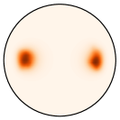
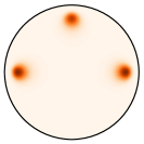
Figure 2: KDE estimation (kernel $e^{-d_{\mathbb{H}}^{2}/\sigma}$) of optimal $(\pi_{1},\pi_{2})$ of $\text{{USOT}}(\alpha,\beta)$ when $\text{D}_{\varphi_{i}}=\rho\text{{KL}}$.

Document classification.

To show the benefits of our proposed losses over SOT, we consider a document classification problem [44]. Documents are represented as distributions of words embedded with word2vec [45] in dimension $d=300$. Let $D_{k}$ be the $k$-th document and $x_{1}^{k},\dots,x_{n_{k}}^{k}\in\mathbb{R}^{d}$ be the set of words in $D_{k}$. Then, $D_{k}=\sum_{i=1}^{n_{k}}w_{i}^{k}\delta_{x_{i}^{k}}$ where $w_{i}^{k}$ is the frequency of $x_{i}^{k}$ in $D_{k}$ normalized s.t. $\sum_{i=1}^{n_{k}}w_{i}^{k}=1$. Given a loss function $\mathrm{L}$, the document classification task is solved by computing the matrix $\big{(}\mathrm{L}(D_{k},D_{\ell})\big{)}_{k,\ell}$, then using a k-nearest neighbor classifier. Since a word typically appears several times in a document, the measures are not uniform and sliced partial OT [28, 29] cannot be used in this setting. The aim of this experiment is to show that by discarding possible outliers using a well chosen parameter $\rho$, USOT is able to outperform SOT and SUOT on this task. We consider three different datasets, BBCSport [44], Movies reviews [46] and the Goodreads dataset [47] on two tasks (genre and likability). We report in Figure 3 the accuracy of SUOT, USOT and the stochastic USOT (SUSOT) compared with SOT, OT and UOT computed with the majorization minimization algorithm [48] or approximated with the Sinkhorn algorithm [34]. All the benchmark methods are computed using the POT library [49]. For sliced methods (SOT, SUOT, USOT and SUSOT), we average over 3 computations of the loss matrix and report the standard deviation in Figure 3. The number of neighbors was selected via cross validation. The results in Figure 3 are reported for $\rho$ yielding the best accuracy, and we display an ablation of this parameter on the BBCSport dataset in Figure 3. We observe that when $\rho$ is tuned, USOT outperforms SOT, just as UOT outperforms OT. Note that OT and UOT cannot be used in large scale settings (typically large documents) as their complexity scale cubically. We report in Appendix C runtimes on the Goodreads dataset. In particular, computing the OT matrix took 3 times longer than computing the USOT matrix on GPU. Morever, we were unable to run UOT using POT on the Movies and Goodreads datasets in a reasonable amount of time, due to their computational complexity.

Table 1: Accuracy on document classification

	BBCSport	Movies	Goodreads genre	Goodreads like
OT	91.64	68.88	52.75	70.60
UOT	96.27	-	-	-
Sinkhorn UOT	93.64	63.8	42.55	66.06
SOT	$89.39_{\pm 0.76}$	$66.95_{\pm 0.45}$	$50.09_{\pm 0.51}$	$65.60_{\pm 0.20}$
SUOT	$90.12_{\pm 0.15}$	$67.84_{\pm 0.37}$	$50.15_{\pm 0.04}$	$66.72_{\pm 0.38}$
USOT	$92.36_{\pm 0.07}$	$69.21_{\pm 0.37}$	$51.87_{\pm 0.56}$	$67.41_{\pm 1.06}$
SUSOT	$92.45_{\pm 0.39}$	$69.53_{\pm 0.53}$	$51.93_{\pm 0.53}$	$67.33_{\pm 0.26}$

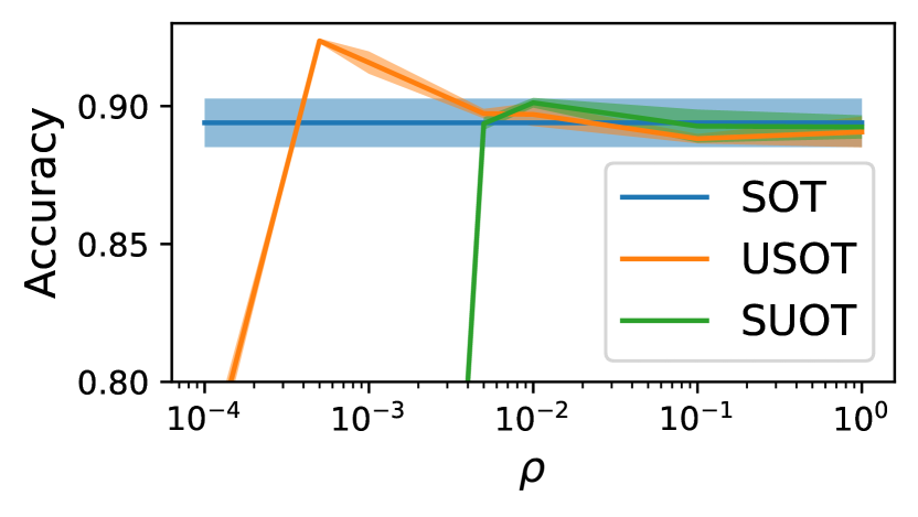
Figure 3: Ablation on BBCSport of the parameter $\rho$.

Barycenter on geophysical data.

OT barycenters are an important topic of interest [37, 50] for their ability to capture mass changes and spatial deformations over several reference measures. In order to compute barycenters under the USOT geometry on a fixed grid, we employ a mirror-descent strategy similar to [51, Algorithm (1)] and described more in depth in Appendix C. We showcase unbalanced sliced OT barycenter using climate model data. Ensembles of multiple models are commonly employed to reduce biases and evaluate uncertainties in climate projections (e.g. [52, 53]). The commonly used Multi-Model Mean approach assumes models are centered around true values and averages the ensemble with equal or varying weights. However, spatial averaging may fail in capturing specific characteristics of the physical system at stake. We propose to use USOT barycenter here instead. We use data from the ClimateNet dataset [54], and more specifically the TMQ (precipitable water) indicator. The ClimateNet dataset is a human-expert-labeled curated dataset that captures notably tropical cyclones (TCs). In order to simulate the output of several climate models, we take a specific instant (first date of 2011) and deform the data with the elastic deformation from TorchVision [41], in an area located close to the eastern part of the United States of America. As a result, we obtain 4 different TCs, as shown in the first row of Figure 4. The classical L2 spatial mean is displayed on the second row of Figure 4 and, as can be expected, reveal 4 different TCs centers/modes, which is undesirable. As the total TMQ mass in the considered zone varies between the different models, a direct application of SOT is impossible, or requires a normalization of the mass that has undesired effect as can be seen on the second picture of the second row. Finally, we show the result of the USOT barycenter with $\rho_{1}=1e1$ (related to the data) and $\rho_{2}=1e4$ (related to the barycenter). As a result, the corresponding barycenter has only one apparent mode which is the expected behaviour. The considered measures have a size of $100\times 200$, and we run the barycenter algorithm for $500$ iterations (with $K=64$ projections), which takes $3$ minutes on a commodity GPU. UOT barycenters for this size of problems are untractable, and to the best of our knowledge, this is the first time such large scale unbalanced OT barycenters can be computed. This experiment encourages an in-depth analysis of the relevance of this aggregation strategy for climate modeling and related problems, which we will investigate as future work.

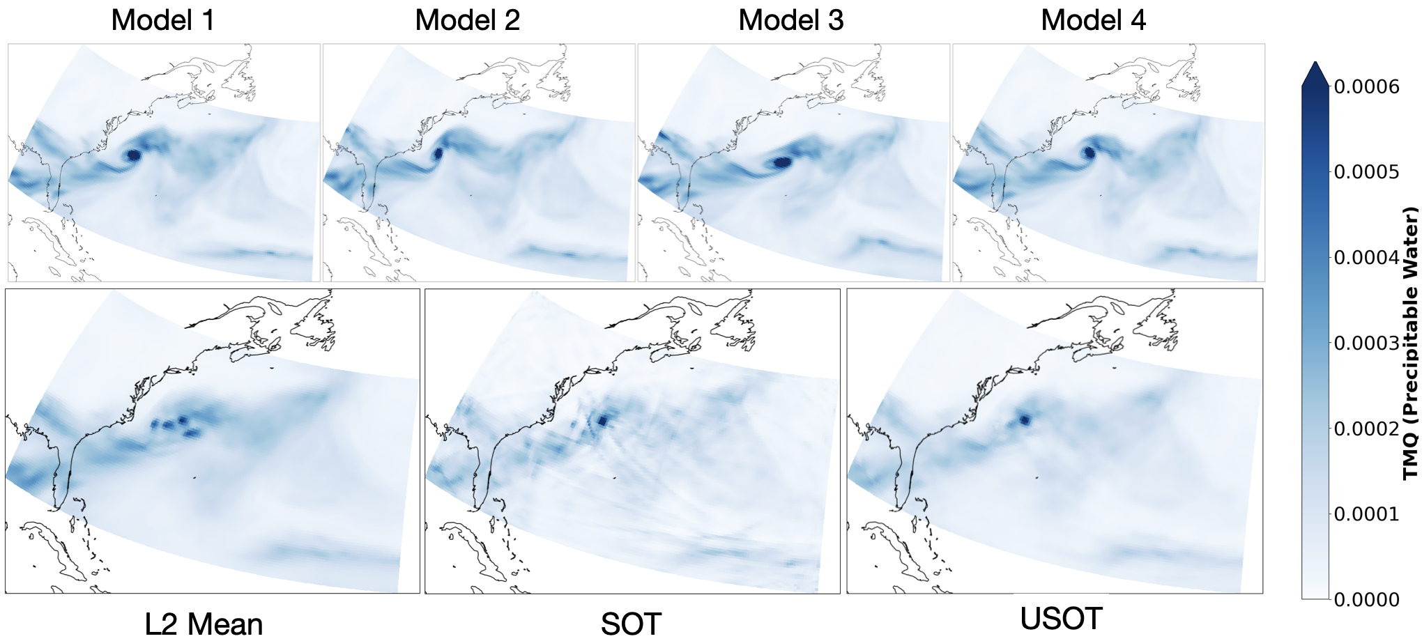
Figure 4: Barycenter of geophysical data. (First row) Simulated output of 4 different climate models depicting different scenarios for the evolution of a tropical cyclone (Second row) Results of different averaging/aggregation strategies.

6 Conclusion and Discussion

We proposed two losses merging unbalanced and sliced OT altogether, with theoretical guarantees and an efficient Frank-Wolfe algorithm which allows to reuse any sliced OT variant. We highlighted experimentally the performance improvement over SOT, and described novel applications of unbalanced OT barycenters of positive measures, with a new case study on geophysical data. These novel results and algorithms pave the way to numerous new applications of sliced variants of OT, and we believe that our contributions will motivate practitioners to further explore their use in general ML applications, without the requirements of manipulating probability measures.

On the limitations side, an immediate drawback arises from the induced additional computational cost w.r.t. SOT. While the above experimental results show that SUOT and USOT improve performance significantly over SOT, and though the complexity is still sub-quadratic in number of samples, our FW approach uses SOT as a subroutine, rendering it necessarily more expensive. Additionally, another practical burden comes from the introduction of extra parameters $(\rho_{1},\rho_{2})$ which requires cross-validation when possible. Therefore, a future direction would be to derive efficient strategies to tune $(\rho_{1},\rho_{2})$, maybe w.r.t. the applicative context, and further complement the possible interpretations of $\rho$ as a ’threshold’ for the geometric information encode by $\text{{C}}_{1}$, $\text{{C}}_{d}$.

On the theoretical side, while OT between univariate measures has been shown to define a reproducing kernel, and while sliced OT can take advantage of this property [55, 56], some of our numerical experiments suggest this property no longer holds for UOT (and therefore, for SUOT and USOT). This negative result leaves as an open direction the design of OT-based kernel methods between arbitrary positive measures.

Appendix A Postponed proofs for Section 3

A.1 Existence of minimizers

We provide the formal statement and detailed proof on the existence of a solution for both SUOT and USOT, as mentioned in Section 3.

Proposition 3.

(Existence of minimizers) Assume that $\text{{C}}_{1}$ is lower-semicontinuous and that either (i) $\varphi_{1,\infty}^{\prime}=\varphi_{2,\infty}^{\prime}=+\infty$, or (ii) $\text{{C}}_{1}$ has compact sublevels on $\mathbb{R}\times\mathbb{R}$ and $\varphi_{1,\infty}^{\prime}+\varphi_{2,\infty}^{\prime}+\inf\text{{C}}_{1}>0$. Then the solution of $\text{{SUOT}}(\alpha,\beta)$ and $\text{{USOT}}(\alpha,\beta)$ exist, i.e. the infimum in (5) and (6) is attained. More precisely, there exists $(\pi_{1},\pi_{2})$ which attains the infimum for $\text{{USOT}}(\alpha,\beta)$ (see Equation (6)). Concerning $\text{{SUOT}}(\alpha,\beta)$, there exists for any $\theta\in\mathrm{supp}(\bm{\sigma})$ a plan $\pi_{\theta}$ attaining the infimum in $\text{{UOT}}(\theta^{\star}_{\sharp}\alpha,\theta^{\star}_{\sharp}\beta)$ (see Equation (2)).

Proof.

We leverage [4, Theorem 3.3] to prove this proposition. In the setting of SUOT, if such assumptions (i) or (ii) are satisfied for $(\alpha,\beta)$, then they also hold for $(\theta^{\star}_{\sharp}\alpha,\theta^{\star}_{\sharp}\beta)$ for any $\theta\in\mathbb{S}^{d-1}$. Hence, $\text{{UOT}}(\theta^{\star}_{\sharp}\alpha,\theta^{\star}_{\sharp}\beta)$ admits a solution $\pi^{\theta}$.

Concerning USOT, note that one necessarily has $m(\pi_{1})=m(\pi_{2})$, otherwise $\text{{SOT}}(\pi_{1},\pi_{2})=+\infty$. From [4, Equation (3.10)], that for any admissible $(\pi_{1},\pi_{2},\pi)$, one has

$$\text{{USOT}}(\alpha,\beta)\geq m(\pi)\inf\text{{C}}_{1}+m(\alpha)\varphi_{1}(\tfrac{m(\pi)}{m(\alpha)})+m(\beta)\varphi_{2}(\tfrac{m(\pi)}{m(\beta)}).$$

In both settings the above bounds implies coercivity of the functional of USOT w.r.t. the masses of the measures $(\pi_{1},\pi_{2},\pi)$. Thus there exists $M>0$ such that $m(\pi_{1})=m(\pi_{2})=m(\pi)<M$, otherwise $\text{{USOT}}(\alpha,\beta)=+\infty$. By the Banach-Alaoglu theorem, the set of bounded measures $(\pi_{1},\pi_{2})$ is compact, and the set of plans $\pi$ with such marginals is also compact because $\mathbb{R}^{d}$ is Polish and $\text{{C}}_{1}$ is lower-semicontinuous [57, Theorem 1.7]. Because the functional of USOT is lower-semicontinuous in $(\pi_{1},\pi_{2},\pi)$ and we can restrict optimization over a compact set, we have existence of minimizers for USOT by standard proofs of calculus of variations. ∎

A.2 Metric properties: Proof of Proposition 2

Proof of Proposition 2.

Metric properties of SUOT. Symmetry and non-negativity are immediate. Assume $\text{{SUOT}}(\alpha,\beta)=0$. Since $\bm{\sigma}$ is the uniform distribution on $\mathbb{S}^{d-1}$, then for any $\theta\in\mathbb{S}^{d-1}$, $\text{{UOT}}(\theta^{\star}_{\sharp}\alpha,\theta^{\star}_{\sharp}\beta)=0$, and since UOT is assumed to be definite, then $\theta^{\star}_{\sharp}\alpha=\theta^{\star}_{\sharp}\beta$. By [58, Proposition 3.8.6], this implies that $\alpha$ and $\beta$ have the same Fourier transform. By injectivity of the Fourier transform, we conclude that $\alpha=\beta$, hence SUOT is definite. The triangle inequality results from applying the Minkowski inequality then the triangle inequality for $\text{{UOT}}^{1/p}$ for $p\in[1,+\infty)$: for any $\alpha,\beta,\gamma\in\mathcal{M}_{+}(\mathbb{R}^{d})$,

$$\text{{SUOT}}^{1/p}(\alpha,\beta)$$

$$=\Bigg{(}\int_{\mathbb{S}^{d-1}}\text{{UOT}}(\theta^{\star}_{\sharp}\alpha,\theta^{\star}_{\sharp}\beta)\mathrm{d}\bm{\sigma}(\theta)\Bigg{)}^{1/p}$$

$$\leq\Bigg{(}\int_{\mathbb{S}^{d-1}}\big{[}\text{{UOT}}^{1/p}(\theta^{\star}_{\sharp}\alpha,\theta^{\star}_{\sharp}\gamma)+\text{{UOT}}^{1/p}(\theta^{\star}_{\sharp}\gamma,\theta^{\star}_{\sharp}\beta)\big{]}^{p}\mathrm{d}\bm{\sigma}(\theta)\Bigg{)}^{1/p}$$

$$\leq\Bigg{(}\int_{\mathbb{S}^{d-1}}\big{[}\text{{UOT}}^{1/p}(\theta^{\star}_{\sharp}\alpha,\theta^{\star}_{\sharp}\gamma)\big{]}^{p}\mathrm{d}\bm{\sigma}(\theta)\Bigg{)}^{1/p}+\Bigg{(}\int_{\mathbb{S}^{d-1}}\big{[}\text{{UOT}}^{1/p}(\theta^{\star}_{\sharp}\gamma,\theta^{\star}_{\sharp}\beta)\big{]}^{p}\mathrm{d}\bm{\sigma}(\theta)\Bigg{)}^{1/p}$$

$$=\text{{SUOT}}^{1/p}(\alpha,\gamma)+\text{{SUOT}}^{1/p}(\gamma,\beta).$$

Metric properties of USOT. Let $(\alpha,\beta)\in\mathcal{M}_{+}(\mathbb{R}^{d})$. Non-negativity is immediate, as USOT is defined as a program minimizing a sum of positive terms. SOT is symmetric, thus when $\varphi_{1}=\varphi_{2}$, we obtain symmetry of the functional w.r.t. $(\alpha,\beta)$. Assume $\text{D}_{\varphi}$ is definite, i.e. $\text{D}_{\varphi}(\alpha|\beta)=0$ implies $\alpha=\beta$. Assume now that $\text{{USOT}}(\alpha,\beta)=0$, and denote by $(\pi_{1},\pi_{2})$ the optimal marginals attaining the infimum in (6). $\text{{USOT}}(\alpha,\beta)=0$ implies that $\text{{SOT}}(\pi_{1},\pi_{2})=0$, $\text{D}_{\varphi}(\pi_{1}|\alpha)=0$ and $\text{D}_{\varphi}(\pi_{2}|\beta)=0$. These three terms are definite, which yields $\alpha=\pi_{1}=\pi_{2}=\beta$, hence the definiteness of USOT.

∎

A.3 Comparison of SUOT, USOT, SOT, and proof of Theorem 1

In this section, we establish several bounds to compare SUOT, USOT and SOT on the space of compactly-supported measures. We provide the detailed derivations and auxiliary lemmas needed for the proofs. Note that Theorem 1 is a direct consequence from Theorems 6, 7 and 8.

Theorem 6.

Let $\mathsf{X}$ be a compact subset of $\mathbb{R}^{d}$ with radius $R$ and consider $\alpha,\beta\in\mathcal{M}_{+}(\mathsf{X})$. Then, $\text{{SUOT}}(\alpha,\beta)\leq\text{{USOT}}(\alpha,\beta)$.

Proof.

To show that $\text{{SUOT}}(\alpha,\beta)\leq\text{{USOT}}(\alpha,\beta)$, we use a sub-optimality argument. Let $\pi$ be the solution $\text{{USOT}}(\alpha,\beta)$ and denote by $(\pi_{1},\pi_{2})$ the marginals of $\pi$. For any $\theta\in\mathbb{S}^{d-1}$, denote by $\pi_{\theta}$ the solution of $\text{{OT}}(\theta^{\star}_{\sharp}\pi_{1},\theta^{\star}_{\sharp}\pi_{2})$. By definition of USOT, the marginals of $\pi_{\theta}$ are given by $(\theta^{\star}_{\sharp}\pi_{1},\theta^{\star}_{\sharp}\pi_{2})$. Since the sequence $(\pi_{\theta})_{\theta}$ is suboptimal for the problem $\text{{SUOT}}(\alpha,\beta)$, one has

$$\text{{SUOT}}(\alpha,\beta) \leq\int_{\mathbb{S}^{d-1}}\big{\{}\int\text{{C}}_{1}\mathrm{d}\pi_{\theta}+\mathrm{D}_{\varphi_{1}}(\theta^{\star}_{\sharp}\pi_{1}|\theta^{\star}_{\sharp}\alpha)+\mathrm{D}_{\varphi_{2}}(\theta^{\star}_{\sharp}\pi_{2}|\theta^{\star}_{\sharp}\beta)\big{\}}\mathrm{d}\bm{\sigma}(\theta)$$ (10)

$$\leq\int_{\mathbb{S}^{d-1}}\int\text{{C}}_{1}\mathrm{d}\pi_{\theta}\mathrm{d}\bm{\sigma}(\theta)+\mathrm{D}_{\varphi_{1}}(\pi_{1}|\alpha)+\mathrm{D}_{\varphi_{2}}(\pi_{2}|\beta)$$ (11)

$$=\text{{USOT}}(\alpha,\beta),$$ (12)

where the second inequality results from Lemma 1, and the last equality follows from the definition of $\text{{USOT}}(\alpha,\beta)$. ∎

Theorem 7.

Let $\mathsf{X}$ be a compact subset of $\mathbb{R}^{d}$ with radius $R$ and consider $\alpha,\beta\in\mathcal{M}_{+}(\mathsf{X})$. Additionally, let $p\in[1,+\infty)$ and assume $\text{{C}}_{1}(x,y)=|x-y|^{p}$ for $(x,y)\in\mathbb{R}\times\mathbb{R}$ and $\text{{C}}_{d}(x,y)=\|x-y\|^{p}$ for $(x,y)\in\mathbb{R}^{d}\times\mathbb{R}^{d}$. Then, $\text{{USOT}}(\alpha,\beta)\leq\text{{UOT}}(\alpha,\beta)$.

Proof.

By [59, Proposition 5.1.3], $\text{{SOT}}(\mu,\nu)\leq K~{}\text{{OT}}(\mu,\nu)$ with $K\leq 1$. Let $\pi$ be the solution of $\text{{UOT}}(\alpha,\beta)$ with marginals $(\pi_{1},\pi_{2})$. These marginals are sub-optimal for $\text{{USOT}}(\alpha,\beta)$, we have

$$\text{{USOT}}(\alpha,\beta) \leq\text{{SOT}}(\pi_{1},\pi_{2})+\mathrm{D}_{\varphi_{1}}(\pi_{1}|\alpha)+\mathrm{D}_{\varphi_{2}}(\pi_{2}|\beta)\,,$$ (13)

$$\leq\text{{OT}}(\pi_{1},\pi_{2})+\mathrm{D}_{\varphi_{1}}(\pi_{1}|\alpha)+\mathrm{D}_{\varphi_{2}}(\pi_{2}|\beta)\,,$$ (14)

$$=\text{{UOT}}(\alpha,\beta)\,,$$ (15)

where the last equality is obtained because $\pi$ is optimal in $\text{{UOT}}(\alpha,\beta)$. ∎

Theorem 8.

Let $\mathsf{X}$ be a compact subset of $\mathbb{R}^{d}$ with radius $R$ and consider $\alpha,\beta\in\mathcal{M}_{+}(\mathsf{X})$. Additionally, let $p\in[1,+\infty)$ and assume $\text{{C}}_{1}(x,y)=|x-y|^{p}$ for $(x,y)\in\mathbb{R}$ and $\text{{C}}_{d}(x,y)=\|x-y\|^{p}$ for $(x,y)\in\mathbb{R}^{d}$. Let $\rho>0$ and assume $D_{\varphi_{1}}=D_{\varphi_{2}}=\rho\text{{KL}}$. Then, $\text{{UOT}}(\alpha,\beta)\leq c\,\text{{SUOT}}(\alpha,\beta)^{1/(d+1)}$, where $c=c(m(\alpha),m(\beta),\rho,R)$ is a non-decreasing function of $m(\alpha)$ and $m(\beta)$.

Proof.

We adapt the proof of [59, Lemma 5.1.4], which establishes a bound between OT and SOT. The first step consists in bounding from above the distance between two regularized measures.

Let $\psi:\mathbb{R}^{d}\to\mathbb{R}_{+}$ be a smooth and radial function verifying $\mathrm{supp}(\psi)\subseteq B_{d}({\bf 0},1)$ and $\int_{\mathbb{R}^{d}}\psi(x)\mathrm{d}\mathrm{Leb}(x)=1$. Let $\psi_{\lambda}(x)=\lambda^{-d}\psi(x/\lambda)/\mathcal{A}(\mathbb{S}^{d-1})$ where $\mathcal{A}(\mathbb{S}^{d-1})$ is the surface area of $\mathbb{S}^{d-1}$, i.e. $\mathcal{A}(\mathbb{S}^{d-1})=\frac{2\pi^{d/2}}{\Gamma(d/2)}$ with $\Gamma$ the gamma function. For any function $f$ defined on $\mathbb{R}^{s}$ ($s\geq 1$), denote by $\mathcal{F}[f]$ the Fourier transform of $f$ defined for $x\in\mathbb{R}^{s}$ as $\mathcal{F}[f](x)=\int_{\mathbb{R}^{s}}f(w)e^{-\mathrm{i}\left\langle w,x\right\rangle}\mathrm{d}w$. Let $\alpha_{\lambda}=\alpha\ast\varphi_{\lambda}$ and $\beta_{\lambda}=\beta\ast\varphi_{\lambda}$ where $\ast$ is the convolution operator. Let $(f,g)$ such that $f\oplus g\leq\text{{C}}_{d}$. By using the isometry properties of the Fourier transform and the definition of $\psi_{\lambda}$, then representing the variables with polar coordinates, we have

$$\int_{\mathbb{R}^{d}}\varphi^{\circ}(f(x))\mathrm{d}\alpha_{\lambda}(x) =\int_{\mathbb{R}^{d}}\mathcal{F}[\varphi^{\circ}\circ f](w)\mathcal{F}[\alpha](w)\mathcal{F}[\psi](\lambda w)\mathrm{d}w$$ (16)

$$=\int_{\mathbb{S}^{d-1}}\int_{0}^{+\infty}\mathcal{F}[\varphi^{\circ}\circ f](r\theta)\mathcal{F}[\alpha](r\theta)\mathcal{F}[\psi](\lambda r)r^{d-1}\mathrm{d}r\mathrm{d}\bm{\sigma}(\theta)\,.$$ (17)

Since $\varphi^{\circ}\circ f$ is a real-valued function, $\mathcal{F}[\varphi^{\circ}\circ f]$ is an even function, then

$$\int_{\mathbb{R}^{d}}\varphi^{\circ}(f(x))\mathrm{d}\alpha_{\lambda}(x)$$ (18)

$$=\frac{1}{2}\int_{\mathbb{S}^{d-1}}\int_{\mathbb{R}}\mathcal{F}[\varphi^{\circ}\circ f](r\theta)\mathcal{F}[\alpha](r\theta)\mathcal{F}[\psi](\lambda r)|r|^{d-1}\mathrm{d}r\mathrm{d}\bm{\sigma}(\theta)$$ (19)

$$=\frac{1}{2}\int_{\mathbb{S}^{d-1}}\int_{\mathbb{R}}\mathcal{F}[\varphi^{\circ}\circ f](r\theta)\mathcal{F}[\theta^{\star}_{\sharp}\alpha](r)\mathcal{F}[\psi](\lambda r)|r|^{d-1}\mathrm{d}r\mathrm{d}\bm{\sigma}(\theta)$$ (20)

$$=\frac{1}{2}\int_{\mathbb{S}^{d-1}}\int_{\mathbb{R}}\mathcal{F}[\varphi^{\circ}\circ f](r\theta)\Bigg{(}\int_{-R}^{R}e^{-\mathrm{i}ru}\mathrm{d}\theta^{\star}_{\sharp}\alpha(u)\Bigg{)}\mathcal{F}[\psi](\lambda r)\left|r\right|^{d-1}\mathrm{d}r\mathrm{d}\bm{\sigma}(\theta)$$ (21)

$$=\frac{1}{2}\int_{\mathbb{S}^{d-1}}\int_{\mathbb{R}}\Bigg{(}\int_{\mathbb{R}^{d}}\int_{-R}^{R}\varphi^{\circ}(f(x))e^{-\mathrm{i}r(u+\langle\theta,x\rangle)}\mathrm{d}\theta^{\star}_{\sharp}\alpha(u)\Bigg{)}\mathcal{F}[\psi](\lambda r)\left|r\right|^{d-1}\mathrm{d}x\mathrm{d}r\mathrm{d}\bm{\sigma}(\theta)\;.$$ (22)

Equation (20) follows from the property of push-forward measures, (21) results from the definition of the Fourier transform and $u\in[-R,R]$, and (22) results from the definition of the Fourier transform and Fubini’s theorem. By making a change of variables ($x$ becomes $x-u\theta$), we obtain

$$\int_{\mathbb{R}^{d}}\varphi^{\circ}(f(x))\mathrm{d}\alpha_{\lambda}(x)$$ (23)

$$=\frac{1}{2}\int_{\mathbb{S}^{d-1}}\int_{\mathbb{R}}\int_{\mathbb{R}^{d}}\int_{-R}^{R}\varphi^{\circ}(f(x-u\theta))e^{-\mathrm{i}r\langle\theta,x\rangle}\mathrm{d}\theta^{\star}_{\sharp}\alpha(u)\mathcal{F}[\psi](\lambda r)\left|r\right|^{d-1}\mathrm{d}x\mathrm{d}r\mathrm{d}\bm{\sigma}(\theta)$$ (24)

$$=\frac{1}{2}\int_{\mathbb{S}^{d-1}}\int_{\mathbb{R}}\int_{B_{d}({\bf 0},2R+\lambda)}\int_{-R}^{R}\varphi^{\circ}(f(x-u\theta))e^{-\mathrm{i}r\langle\theta,x\rangle}\mathrm{d}\theta^{\star}_{\sharp}\alpha(u)\mathcal{F}[\psi](\lambda r)\left|r\right|^{d-1}\mathrm{d}x\mathrm{d}r\mathrm{d}\bm{\sigma}(\theta)\;,$$ (25)

where (25) follows from the assumption that $\mathrm{supp}(\alpha)\subseteq B_{d}({\bf 0},R)$. Indeed, this implies that $\mathrm{supp}(\alpha_{\lambda})\subseteq B_{d}({\bf 0},R+\lambda)$, thus the domain of $x\mapsto\varphi^{\circ}\circ f(x-u\theta)$ is contained in $B_{d}({\bf 0},2R+\lambda)$.

Similarly, one can show that

$$\int_{\mathbb{R}^{d}}\varphi^{\circ}(g(y))\mathrm{d}\beta_{\lambda}(y)$$ (26)

$$=\frac{1}{2}\int_{\mathbb{S}^{d-1}}\int_{\mathbb{R}}\int_{B_{d}({\bf 0},2R+\lambda)}\int_{-R}^{R}\varphi^{\circ}(g(y-u\theta))e^{-\mathrm{i}r\langle\theta,y\rangle}\mathrm{d}\theta^{\star}_{\sharp}\beta(u)\mathcal{F}[\psi](\lambda r)\left|r\right|^{d-1}\mathrm{d}y\mathrm{d}r\mathrm{d}\bm{\sigma}(\theta)\;.$$ (27)

By (25) and (27), and applying Fubini’s theorem, we obtain

$$\int_{\mathbb{R}^{d}}\varphi^{\circ}(f(x))\mathrm{d}\alpha_{\lambda}(x)+\int_{\mathbb{R}^{d}}\varphi^{\circ}(g(y))\mathrm{d}\beta_{\lambda}(y)$$ (28)

$$\leq\frac{1}{2}\int_{\mathbb{R}}\int_{B_{d}({\bf 0},2R+\lambda)}\int_{\mathbb{S}^{d-1}}\Big{\{}\int_{-R}^{R}\varphi^{\circ}(f(x-u\theta))\mathrm{d}\theta^{\star}_{\sharp}\alpha(u)$$

$$\qquad\qquad\qquad\qquad\qquad+\int_{-R}^{R}\varphi^{\circ}(g(x-u\theta))\mathrm{d}\theta^{\star}_{\sharp}\beta(u)\Big{\}}e^{-\mathrm{i}r\langle\theta,x\rangle}\mathcal{F}[\psi](\lambda r)\left|r\right|^{d-1}\mathrm{d}\bm{\sigma}(\theta)\mathrm{d}x\mathrm{d}r$$ (29)

$$\leq c_{1}(2R+\lambda)^{d}\int_{\mathbb{S}^{d-1}}\text{{UOT}}(\theta^{\star}_{\sharp}\alpha,\theta^{\star}_{\sharp}\beta)\mathrm{d}\bm{\sigma}(\theta)\int_{\mathbb{R}}\lambda^{-d}\big{|}\mathcal{F}[\psi](r)\left|r\right|^{d-1}\big{|}\mathrm{d}r$$ (30)

$$\leq c_{2}(2R+\lambda)^{d}\lambda^{-d}\text{{SUOT}}(\alpha,\beta)$$ (31)

where $c_{1}>0$ is independent from $\alpha$ and $\beta$, and $c_{2}=c_{1}\int_{\mathbb{R}}\big{|}\mathcal{F}[\psi](r)\big{|}\left|r\right|^{d-1}\mathrm{d}r$. Equation (31) is obtained by taking the supremum of (29) over the set of potentials $(\tilde{f},\tilde{g})$ such that for $u\in[-R,R]$, $\exists(x,\theta)\in B_{d}({\bf 0},2R+\lambda)\times\mathbb{S}^{d-1}$, $\tilde{f}(u)=f(x-u\theta),\,\tilde{g}(u)=g(x-u\theta)$, which is included in the set of potentials $(f^{\prime},g^{\prime})$ s.t. $f^{\prime}:\mathbb{R}\to\mathbb{R}$, $g^{\prime}:\mathbb{R}\to\mathbb{R}$ and $f^{\prime}\oplus g^{\prime}\leq\text{{C}}_{1}$.

We deduce from the dual formulation of UOT (3) and (31) that,

$$\text{{UOT}}(\alpha_{\lambda},\beta_{\lambda})\leq c_{2}(2R+\lambda)^{d}\lambda^{-d}\text{{SUOT}}(\alpha,\beta)\,.$$ (32)

The last step of the proof consists in relating $\text{{UOT}}(\alpha_{\lambda},\beta_{\lambda})$ with $\text{{UOT}}(\alpha,\beta)$. For any $(f,g)$ such that $f\oplus g\leq\text{{C}}_{d}$, we have

$$\int_{\mathbb{R}^{d}}\varphi^{\circ}(f(x))\mathrm{d}\alpha(x)+\int_{\mathbb{R}^{d}}\varphi^{\circ}(g(y))\mathrm{d}\beta(y)-\text{{UOT}}(\alpha_{\lambda},\beta_{\lambda})$$ (33)

$$\leq\int_{\mathbb{R}^{d}}\varphi^{\circ}(f(x))\mathrm{d}\alpha(x)+\int_{\mathbb{R}^{d}}\varphi^{\circ}(g(x))\mathrm{d}\beta(x)-\int_{\mathbb{R}^{d}}\varphi^{\circ}(f(x))\mathrm{d}\alpha_{\lambda}(x)-\int_{\mathbb{R}^{d}}\varphi^{\circ}(g(y))\mathrm{d}\beta_{\lambda}(y)$$ (34)

$$\leq\int_{\mathbb{R}^{d}}\{\varphi^{\circ}(f(x))-\psi_{\lambda}\ast\varphi^{\circ}(f(x))\}\mathrm{d}\alpha(x)+\int_{\mathbb{R}^{d}}\{\varphi^{\circ}(g(y))-\psi_{\lambda}\ast\varphi^{\circ}(g(y))\}\mathrm{d}\beta(y)\,.$$ (35)

For $x\in\mathbb{R}^{d}$,

$$\varphi^{\circ}(f(x))-\psi_{\lambda}\ast\varphi^{\circ}(f(x)) =\frac{\lambda^{-d}}{\mathcal{A}(\mathbb{S}^{d-1})}\int_{\mathbb{R}^{d}}\big{(}\varphi^{\circ}(f(x))-\varphi^{\circ}(f(y))\big{)}\psi\left(\frac{x-y}{\lambda}\right)\mathrm{d}y$$ (36)

$$\leq\frac{\lambda^{-d}}{\mathcal{A}(\mathbb{S}^{d-1})}\int_{\mathbb{R}^{d}}\bigl{|}\varphi^{\circ}(f(x))-\varphi^{\circ}(f(y))\bigr{|}\psi\left(\frac{x-y}{\lambda}\right)\mathrm{d}y\,,$$ (37)

Since $\text{D}_{\varphi}=\rho\text{{KL}}$, then for $z\in\mathbb{R}$, $\varphi^{\circ}(z)=\rho(1-e^{-z/\rho})$, so for $(x,y)\in\mathbb{R}^{d}\times\mathbb{R}^{d}$,

$$\varphi^{\circ}(f(x))-\varphi^{\circ}(f(y)) =\rho(e^{-f(y)/\rho}-e^{-f(x)/\rho})$$ (38)

By Lemma 4, the potentials $(f,g)$ are bounded by constants depending on $m(\alpha),m(\beta)$, thus we can bound (38) as follows.

$$|\varphi^{\circ}(f(x))-\varphi^{\circ}(f(y))|\leq\rho e^{-\lambda^{\star}/\rho}\left(1-e^{-R/\rho}\right)\,,$$ (39)

with $\lambda^{\star}\in[-R+\frac{\rho}{2}\log\frac{m(\alpha)}{m(\beta)},\frac{R}{2}+\frac{\rho}{2}\log\frac{m(\alpha)}{m(\beta)}]$. We thus derive the following upper-bound on (37).

$$\varphi^{\circ}(f(x))-\psi_{\lambda}\ast\varphi^{\circ}(f(x)) \leq\frac{\lambda^{-d}}{\mathcal{A}(\mathbb{S}^{d-1})}\rho e^{-\lambda^{\star}/\rho}\left(1-e^{-R/\rho}\right)\int_{\mathbb{R}^{d}}\psi\left(\frac{x-y}{\lambda}\right)\mathrm{d}y$$ (40)

$$\leq\frac{\lambda^{-d+1}}{\mathcal{A}(\mathbb{S}^{d-1})}\rho e^{-\lambda^{\star}/\rho}\left(1-e^{-R/\rho}\right)\int_{\mathbb{R}^{d}}\frac{1}{\lambda}\psi\left(\frac{x-y}{\lambda}\right)\mathrm{d}y$$ (41)

$$\leq\frac{\lambda^{-d+1}}{\mathcal{A}(\mathbb{S}^{d-1})}\sqrt{\frac{m(\beta)}{m(\alpha)}}\rho e^{R/\rho}\left(1-e^{-R/\rho}\right)\int_{\mathbb{R}^{d}}\frac{1}{\lambda}\psi\left(\frac{x-y}{\lambda}\right)\mathrm{d}y$$ (42)

By doing the change of variables $z=(y-x)/\lambda$ and using the fact that $\psi$ is a radial function and $\int_{\mathbb{R}^{d}}\psi(z)\mathrm{d}\mathrm{Leb}(z)=1$, we obtain $\int_{\mathbb{R}^{d}}\frac{1}{\lambda}\psi\left(\frac{x-y}{\lambda}\right)\mathrm{d}y=1$. Therefore,

$$\varphi^{\circ}(f(x))-\psi_{\lambda}\ast\varphi^{\circ}(f(x)) \leq\frac{\lambda^{-d+1}}{\mathcal{A}(\mathbb{S}^{d-1})}\sqrt{\frac{m(\beta)}{m(\alpha)}}\rho e^{R/\rho}\left(1-e^{-R/\rho}\right)$$ (43)

$$\leq\frac{\lambda}{\mathcal{A}(\mathbb{S}^{d-1})}\sqrt{\frac{m(\beta)}{m(\alpha)}}\rho e^{R/\rho}\left(1-e^{-R/\rho}\right)\,.$$ (44)

Similarly, using the bounds on $g$ in Lemma 4, one can show that

$$|\varphi^{\circ}(g(x))-\varphi^{\circ}(g(y))|\leq\rho e^{\lambda^{\star}/\rho}\left(e^{R/\rho}-e^{-R/\rho}\right)\leq\rho\sqrt{\frac{m(\alpha)}{m(\beta)}}e^{R/2\rho}\left(e^{R/\rho}-e^{-R/\rho}\right)\,,$$ (45)

therefore,

$$\varphi^{\circ}(g(x))-\psi_{\lambda}\ast\varphi^{\circ}(g(x)) \leq\frac{\lambda}{\mathcal{A}(\mathbb{S}^{d-1})}\sqrt{\frac{m(\alpha)}{m(\beta)}}\rho e^{R/2\rho}\left(e^{R/\rho}-e^{-R/\rho}\right)\,.$$ (46)

We conclude that,

$$\int_{\mathbb{R}^{d}}\varphi^{\circ}(f(x))\mathrm{d}\alpha(x)+\int_{\mathbb{R}^{d}}\varphi^{\circ}(g(y))\mathrm{d}\beta(y)-\text{{UOT}}(\alpha_{\lambda},\beta_{\lambda})$$ (47)

$$\leq\frac{\lambda\rho}{\mathcal{A}(\mathbb{S}^{d-1})}\left\{m(\alpha)e^{-\lambda^{\star}/\rho}\left(1-e^{-R/\rho}\right)+m(\beta)e^{\lambda^{\star}/\rho}\left(e^{R/\rho}-e^{-R/\rho}\right)\right\}$$ (48)

$$\leq\frac{\lambda\rho}{\mathcal{A}(\mathbb{S}^{d-1})}\sqrt{m(\alpha)m(\beta)}\left\{e^{R/\rho}\left(1-e^{-R/\rho}\right)+e^{R/2\rho}\left(e^{R/\rho}-e^{-R/\rho}\right)\right\}$$ (49)

Taking the supremum on both sides over $(f,g)$ such that $f\oplus g\leq\text{{C}}_{d}$ yields,

$$\text{{UOT}}(\alpha,\beta)-\text{{UOT}}(\alpha_{\lambda},\beta_{\lambda})$$ (50)

$$\leq\frac{\lambda\rho}{\mathcal{A}(\mathbb{S}^{d-1})}\left\{m(\alpha)e^{-\lambda^{\star}/\rho}\left(1-e^{-R/\rho}\right)+m(\beta)e^{\lambda^{\star}/\rho}\left(e^{R/\rho}-e^{-R/\rho}\right)\right\}\,$$ (51)

$$\leq\frac{\lambda\rho}{\mathcal{A}(\mathbb{S}^{d-1})}\sqrt{m(\alpha)m(\beta)}\left\{e^{R/\rho}\left(1-e^{-R/\rho}\right)+e^{R/2\rho}\left(e^{R/\rho}-e^{-R/\rho}\right)\right\}.$$ (52)

Finally, by combining (32) with the above inequality, we obtain

$$\text{{UOT}}(\alpha,\beta)$$ (53)

$$\leq\frac{\lambda\rho}{\mathcal{A}(\mathbb{S}^{d-1})}\sqrt{m(\alpha)m(\beta)}\left\{e^{R/\rho}\left(1-e^{-R/\rho}\right)+e^{R/2\rho}\left(e^{R/\rho}-e^{-R/\rho}\right)\right\}$$ (54)

$$\qquad+c_{2}(2R+\lambda)^{d}\lambda^{-d}\text{{SUOT}}(\alpha,\beta)$$ (55)

$$\leq c\lambda\big{(}1+(2R+\lambda)^{d}\lambda^{-(d+1)}\text{{SUOT}}(\alpha,\beta)\big{)}\,,$$ (56)

where $c$ is a constant satisfying $c\geq c_{2}$ and

$$c\geq\rho\sqrt{m(\alpha)m(\beta)}\left\{e^{R/\rho}\left(1-e^{-R/\rho}\right)+e^{R/2\rho}\left(e^{R/\rho}-e^{-R/\rho}\right)\right\}/\mathcal{A}(\mathbb{S}^{d-1}).$$ (57)

We conclude the proof by plugging $\lambda=R^{d/(d+1)}\text{{SUOT}}(\alpha,\beta)^{1/(d+1)}$ in (56) and using the fact that $\text{{SUOT}}(\alpha,\beta)$ is bounded from above: $\text{{SUOT}}(\alpha,\beta)\leq\rho(m(\alpha)+m(\beta))$ since on the one hand, $\pi$ is suboptimal in (3) thus $\text{{UOT}}(\alpha,\beta)\leq\rho(m(\alpha)+m(\beta))$, and on the other hand, $m(\alpha)=m(\theta^{\star}_{\sharp}\alpha)$ for any $\theta\in\mathbb{S}^{d-1}$. ∎

Lemma 1.

For any $\theta\in\mathbb{S}^{d-1}$ and $\alpha,\beta\in\mathcal{M}_{+}(\mathbb{R}^{d})$, $\text{D}_{\varphi}(\theta^{\star}_{\sharp}\alpha|\theta^{\star}_{\sharp}\beta)\leq\text{D}_{\varphi}(\alpha|\beta)$.

Proof.

For $\alpha,\beta\in\mathcal{M}_{+}(\mathbb{R}^{s})$ with $s\geq 1$, the dual characterization of $\varphi$-divergences reads [4, Theorem 2.7]

$$\text{D}_{\varphi}(\alpha|\beta)=\sup_{f\in\mathcal{E}(\mathbb{R}^{s})}\int_{\mathbb{R}^{s}}\varphi^{\circ}(f(x))\mathrm{d}\beta(x)-\int_{\mathbb{R}^{s}}f(x)\mathrm{d}\alpha(x),$$

where $\mathcal{E}(\mathbb{R}^{s})$ denotes the space of lower semi-continuous functions from $\mathbb{R}^{s}$ to $\mathbb{R}\cup\{+\infty\}$. Therefore, for any $\theta\in\mathbb{S}^{d-1}$ and $\alpha,\beta\in\mathcal{M}_{+}(\mathbb{R}^{d})$,

$$\text{D}_{\varphi}(\theta^{\star}_{\sharp}\alpha|\theta^{\star}_{\sharp}\beta) =\sup_{f\in\mathcal{E}(\mathbb{R})}\int_{\mathbb{R}}\varphi^{\circ}(f(t))\mathrm{d}(\theta^{\star}_{\sharp}\beta)(t)-\int_{\mathbb{R}}f(t)\mathrm{d}(\theta^{\star}_{\sharp}\alpha)(t)$$ (58)

$$=\sup_{g:\mathbb{R}^{d}\to\mathbb{R}\,s.t.\,\exists f\in\mathcal{E}(\mathbb{R}),\,g=f\circ\theta^{\star}}\int_{\mathbb{R}^{d}}\varphi^{\circ}(g(x))\mathrm{d}\beta(x)-\int_{\mathbb{R}^{d}}g(x)\mathrm{d}\alpha(x)$$ (59)

where (59) results from the definition of push-forward measures. We conclude the proof by observing that the supremum in (59) is taken over a subset of $\mathcal{E}(\mathbb{R}^{d})$. ∎

Lemma 2.

[57, Proposition 1.11] Let $p\in[1,+\infty)$ and assume $\text{{C}}_{d}(x,y)=\|x-y\|^{p}$. Let $\alpha,\beta$ with compact support, such that $\text{{C}}_{d}(x,y)\leq R^{p}$ for $(x,y)\in\mathrm{supp}(\alpha)\times\mathrm{supp}(\beta)$. Then without loss of generality the dual potentials $(f,g)$ of $\text{{UOT}}(\alpha,\beta)$ satisfy $f(x)\in[0,R]$ and $g(y)\in[-R,R]$.

Lemma 3.

[31, Proposition 2] Define the translation-invariant dual formulation

$$\text{{UOT}}(\alpha,\beta)=\sup_{f\oplus g\leq\text{{C}}_{d}}\sup_{\lambda\in\mathbb{R}}\int\varphi_{1}^{\circ}(f+\lambda)\mathrm{d}\alpha+\int\varphi_{2}^{\circ}(g-\lambda)\mathrm{d}\beta.$$ (60)

Let $\rho>0$ and assume $\text{D}_{\varphi_{1}}=\text{D}_{\varphi_{2}}=\rho\text{{KL}}$. Take optimal potentials $(f,g)$ in (60). Then optimal potentials in (3) are given by $(f+\lambda^{\star}(f,g),g-\lambda^{\star}(f,g))$, where the optimal translation $\lambda^{\star}$ reads

$$\lambda^{\star}(f,g)\triangleq\frac{1}{2}\Bigg{[}\text{{S}}^{\beta}_{\rho}(g)-\text{{S}}^{\alpha}_{\rho}(f)\Bigg{]},\quad\text{{S}}^{\alpha}_{\rho}(f)\triangleq-\rho\log\int e^{-f/\rho}\mathrm{d}\alpha,$$

and we call $\text{{S}}^{\alpha}_{\rho}(f)$ the soft-minimum of $f$. When $m(\alpha)=1$ and $m\leq f(x)\leq M$, then $m\leq\text{{S}}^{\alpha}_{\rho}(f)\leq M$.

Lemma 4.

Assume $(\alpha,\beta)$ have compact support such that, for $(x,y)\in\mathrm{supp}(\alpha)\times\mathrm{supp}(\beta)$, $C(x,y)\leq R$. Then, without loss of generality, one can restrict the optimization of the dual formulation (3) of $\text{{UOT}}(\alpha,\beta)$ over the set of potentials satisfying for $(x,y)\in\mathrm{supp}(\alpha)\times\mathrm{supp}(\beta)$,

$$f(x)\in[\lambda^{\star},\lambda^{\star}+R]\,,\quad g(y)\in[-\lambda^{\star}-R,-\lambda^{\star}+R]\,,$$

where $\lambda^{\star}\in[-R+\tfrac{\rho}{2}\log\tfrac{m(\alpha)}{m(\beta)},\tfrac{R}{2}+\tfrac{\rho}{2}\log\tfrac{m(\alpha)}{m(\beta)}]$. In particular, one has

$$f(x)\in[-R+\tfrac{\rho}{2}\log\tfrac{m(\alpha)}{m(\beta)},\tfrac{3R}{2}+\tfrac{\rho}{2}\log\tfrac{m(\alpha)}{m(\beta)}]\,,\quad g(y)\in[-\tfrac{3R}{2}-\tfrac{\rho}{2}\log\tfrac{m(\alpha)}{m(\beta)},2R-\tfrac{\rho}{2}\log\tfrac{m(\alpha)}{m(\beta)}]$$

Proof.

Consider the translation-invariant dual formulation (60): if $(f,g)$ are optimal, then for any $\lambda\in\mathbb{R}$, $(f+\lambda,g-\lambda)$ are also optimal. We leverage the structure of the dual constraint $f\oplus g\leq\text{{C}}_{d}$ with Lemma 2. Since for $(x,y)\in\mathrm{supp}(\alpha)\times\mathrm{supp}(\beta)$, $\text{{C}}_{d}(x,y)\leq R$, then without loss of generality, $f(x)\in[0,R]$ and $g(y)\in[-R,R]$. The potentials $(f,g)$ are optimal for the translation-invariant dual energy, and we need a bound for the original dual functional (3). To this end, we leverage Lemma 3 to compute the optimal translation, such that $(f,g)=(f+\lambda^{\star}(f,g),g-\lambda^{\star}(f,g))$. Let $\bar{\alpha}=\alpha/m(\alpha)$ and $\bar{\beta}=\beta/m(\beta)$ be the normalized probability measures. The translation can be written as,

$$\lambda^{\star}(f,g)=\frac{1}{2}\Bigg{[}\text{{S}}^{\bar{\beta}}_{\rho}(g)-\text{{S}}^{\bar{\alpha}}_{\rho}(f)\Bigg{]}+\frac{\rho}{2}\log\frac{m(\alpha)}{m(\beta)},$$ (61)

where the functional $\text{{S}}^{\alpha}_{\rho}$ is defined in Lemma 3. Since $\bar{\alpha}$ and $\bar{\beta}$ are probability measures, then by [60, Proposition 1], $f(x)\in[0,R]$ and $g(x)\in[-R,R]$ respectively imply $\text{{S}}^{\bar{\alpha}}_{\rho}(f)\in[0,R]$ and $\text{{S}}^{\bar{\beta}}_{\rho}(g)\in[-R,R]$. Combining these bounds on $\text{{S}}^{\bar{\alpha}}_{\rho}(f),\ \text{{S}}^{\bar{\beta}}_{\rho}(g)$ with the expression of $\lambda^{\star}(f,g)$ (61) yields the desired bounds on the optimal potentials $(f,g)$ of the dual formulation (3). ∎

A.4 Metrizing weak^∗ convergence: Proof of Theorem 2

Proof.

Let $(\alpha_{n})$ be a sequence of measures in $\mathcal{M}_{+}(\mathsf{X})$ and $\alpha\in\mathcal{M}_{+}(\mathsf{X})$, where $\mathsf{X}\subset\mathbb{R}^{d}$ is compact with radius $R>0$. First, we assume that $\alpha_{n}\rightharpoonup\alpha$. Then, by [4, Theorem 2.25], under our assumptions, $\alpha_{n}\rightharpoonup\alpha$ is equivalent to $\lim_{n\to+\infty}\text{{UOT}}(\alpha_{n},\alpha)=0$. This implies that $\lim_{n\to+\infty}\text{{SUOT}}(\alpha_{n},\alpha)=0$ and $\lim_{n\to+\infty}\text{{USOT}}(\alpha_{n},\alpha)=0$, since by Theorem 1 and non-negativity of SUOT (Proposition 2),

$$0\leq\text{{SUOT}}(\alpha_{n},\alpha)\leq\text{{USOT}}(\alpha_{n},\alpha)\leq\text{{UOT}}(\alpha_{n},\alpha)\,.$$

Conversely, assume either that $\lim_{n\to+\infty}\text{{SUOT}}(\alpha_{n},\alpha)=0$ or $\lim_{n\to+\infty}\text{{USOT}}(\alpha_{n},\alpha)=0$. First assume there exists $M>0$ such that for large enough $n\in\mathbb{N}^{*},m(\alpha_{n})\leq M$, then by Theorem 1, there exists $c>0$ such that $\text{{UOT}}(\alpha_{n},\alpha)\leq c\big{(}\text{{SUOT}}(\alpha_{n},\alpha)\big{)}^{1/(d+1)}$. Since $c$ is doesn’t depend on the masses $(m(\alpha_{n}),m(\alpha))$, it does not depend on $n$. By Theorem 1, it yields metric equivalence between SUOT, USOT and UOT, thus $\lim_{n\to+\infty}\text{{UOT}}(\alpha_{n},\alpha)=0$. By [4, Theorem 2.25], we eventually obtain $\alpha_{n}\rightharpoonup\alpha$, which is the desired result.

The remaining step thus consists in proving that the sequence of masses $(m(\alpha_{n}))_{n\in\mathbb{N}^{*}}$ is indeed uniformly bounded by $M>0$ for large enough $n$. Note that for any $(\alpha,\beta)\in\mathcal{M}_{+}(\mathbb{R}^{d})$, one has $\text{{UOT}}(\alpha,\beta)\geq\rho(\sqrt{m(\alpha)}-\sqrt{m(\beta)})^{2}$. Indeed one has $\text{{UOT}}(\alpha,\beta)\geq\mathcal{D}(\lambda,-\lambda)$, where $\mathcal{D}$ denotes the dual functional (3) and $\lambda=\tfrac{\rho}{2}\log\tfrac{m(\alpha)}{m(\beta)}$. Note that the pair $(\lambda,-\lambda)$ are feasible dual potentials for the constraint $f\oplus g\leq\text{{C}}_{d}$, because the cost $\text{{C}}_{d}$ is positive in our setting. The property of push-forwards measures means that for any $\theta\in\mathbb{S}^{d-1}$, one has $m(\theta^{\star}_{\sharp}\alpha)=m(\alpha)$. Therefore, we obtain the following bounds for $n$ large enough.

$$\text{{USOT}}(\alpha_{n},\alpha)\geq\text{{SUOT}}(\alpha_{n},\alpha) \geq\int_{\mathbb{S}^{d-1}}\rho\bigg{(}\sqrt{m(\theta^{\star}_{\sharp}\alpha_{n})}-\sqrt{m(\theta^{\star}_{\sharp}\alpha)}\bigg{)}^{2}\mathrm{d}\bm{\sigma}(\theta),$$

$$=\rho(\sqrt{m(\alpha_{n})}-\sqrt{m(\alpha)})^{2}.$$

Hence, $\lim_{n\to+\infty}\text{{SUOT}}(\alpha_{n},\alpha)=0$ or $\lim_{n\to+\infty}\text{{USOT}}(\alpha_{n},\alpha)=0$ implies $\lim_{n\to+\infty}m(\alpha_{n})=m(\alpha)$. In other terms the mass of sequence converges and is thus uniformly bounded for large enough $n$. Since we proved that $m(\alpha_{n})<M$ and $m(\alpha)$ is finite, it ends the proof. ∎

A.5 Application to sliced partial OT: Proof of Theorem 3

The proof of Theorem 3 relies on a formulation for SUOT and USOT when $\text{D}_{\varphi_{1}}=\text{D}_{\varphi_{2}}=\rho\text{{TV}}$, which we prove below. Equation (62) is proved in [61], and can then be applied to SUOT. We include it for completeness. Equation (63) is our contribution and is specific to USOT.

Lemma 5.

Let $\rho>0$ and assume $\text{D}_{\varphi_{1}}=\text{D}_{\varphi_{2}}=\rho\text{{TV}}$ and $\text{{C}}_{d}(x,y)=||x-y||$. Then, for any $(\alpha,\beta)\in\mathcal{M}_{+}(\mathbb{R}^{d})$,

$$\text{{UOT}}(\alpha,\beta)=\sup_{f\in\mathcal{E}}\int f(x)\mathrm{d}(\alpha-\beta)(x),$$ (62)

where

$$\mathcal{E}=\{f:\mathbb{R}^{d}\rightarrow\mathbb{R},\,\,||f||_{Lip}\leq 1,\;||f||_{\infty}\leq\rho\},$$

and $||f||_{\infty}\triangleq\sup_{x\in\mathbb{R}^{d}}|f(x)|$ and $||f||_{Lip}\triangleq\sup_{(x,y)\in\mathbb{R}^{d}}\tfrac{|f(x)-f(y)|}{\text{{C}}_{d}(x,y)}$.

Furthermore, for $\text{{C}}_{1}(x,y)=|x-y|$ and an empirical approximation $\hat{\bm{\sigma}}_{N}=\tfrac{1}{N}\sum_{i=1}^{N}\delta_{\theta_{i}}$ of $\bm{\sigma}$, one has

$$\text{{USOT}}(\alpha,\beta)=\sup_{(f_{\theta})\in\mathcal{E}}\int_{\mathbb{R}^{d}}\bigg{(}\int_{\mathbb{S}^{d-1}}f_{\theta}(\theta^{\star}(x))\mathrm{d}\hat{\bm{\sigma}}_{N}(\theta)\bigg{)}\mathrm{d}(\alpha-\beta)(x)\,,$$ (63)

where

$$\mathcal{E}=\{\forall\theta\in\mathrm{supp}(\hat{\bm{\sigma}}_{N}),\,\,f_{\theta}:\mathbb{R}\rightarrow\mathbb{R},\,\,||f_{\theta}||_{Lip}\leq 1,\;||\int_{\mathbb{S}^{d-1}}f_{\theta}\circ\theta^{\star}\mathrm{d}\hat{\bm{\sigma}}_{N}(\theta)||_{\infty}\leq\rho\},$$

and the Lipschitz norm here is defined w.r.t. $\text{{C}}_{1}$ as $||f||_{Lip}\triangleq\sup_{(x,y)\in\mathbb{R}^{d}}\tfrac{|f(x)-f(y)|}{\text{{C}}_{1}(x,y)}$

Proof.

We start with the formulation of Equation 3 and Theorem 5. For USOT one has

$$\text{{USOT}}(\alpha,\beta)=\sup_{f_{\theta}(\cdot)\oplus g_{\theta}(\cdot)\leq\text{{C}}_{1}} \int\varphi_{1}^{\circ}\Big{(}\int_{\mathbb{S}^{d-1}}f_{\theta}(\theta^{\star}(x))\mathrm{d}\sigma_{N}(\theta)\Big{)}\mathrm{d}\alpha(x)$$

$$+\int\varphi_{2}^{\circ}\Big{(}\int_{\mathbb{S}^{d-1}}g_{\theta}(\theta^{\star}(y))\mathrm{d}\sigma_{N}(\theta)\Big{)}\mathrm{d}\beta(y)\,.$$

When $\text{D}_{\varphi}=\rho\text{{TV}}$, the function $\varphi^{\circ}$ reads $\varphi^{\circ}(x)=x$ for $x\in[-\rho,\rho]$, $\varphi^{\circ}(x)=\rho$ when $x\geq\rho$, and $\varphi^{\circ}(x)=-\infty$ otherwise. Noting $f_{avg}(x)=\int_{\mathbb{S}^{d-1}}f_{\theta}(\theta^{\star}(x))\mathrm{d}\sigma_{N}(\theta)$ and $g_{avg}(x)=\int_{\mathbb{S}^{d-1}}g_{\theta}(\theta^{\star}(x))\mathrm{d}\sigma_{N}(\theta)$. This formula on $\varphi^{\circ}$ imposes $f_{avg}(x)\geq-\rho$ and $g_{avg}(x)\geq-\rho$. Furthermore, since we perform a supremum w.r.t. $(f_{avg},g_{avg})$ where $\varphi^{\circ}$ attains a plateau, then without loss of generality, we can impose the constraint $f_{avg}(x)\leq\rho$ and $g_{avg}(x)\geq\rho$, as it will have no impact on the optimal dual functional value. Thus we have that $||f_{avg}||_{\infty}\leq\rho$ and $||g_{avg}||_{\infty}\leq\rho$. To obtain the Lipschitz property, we use the constraint that $f_{\theta}(\cdot)\oplus g_{\theta}(\cdot)\leq\text{{C}}_{1}$ for any $\theta\in\mathrm{supp}(\sigma_{N})$, as well as [57, Proposition 3.1]. Thus by using c-transform for the cost $\text{{C}}_{1}(x,y)=|x-y|$, we can take w.l.o.g $f_{\theta}(\cdot)=-g_{\theta}(\cdot)$ with $f_{\theta}(\cdot)$ a $1$-Lipschitz function. Thus w.l.o.g we can perform the supremum over $(f_{\theta})_{\theta}\in\mathcal{E}$, and rephrase the functional as desired, since we have that $\varphi^{\circ}(f_{avg})=f_{avg}$.

The proof for UOT is exactly the same, except that our inputs are $(f,g)$ instead of $(f_{\theta},g_{\theta})$. ∎

We can now prove Theorem 3.

Proof of Theorem 3.

First we prove that in that setting USOT is a metric. Reusing Lemma 5, we have that for any measures $(\alpha,\beta,\gamma)$

$$\text{{USOT}}(\alpha,\gamma) =\sup_{(f_{\theta})_{\theta}\in\mathcal{E}}\int\bigg{(}\int_{\mathbb{S}^{d-1}}f_{\theta}(\theta^{\star}(x))\mathrm{d}\sigma_{N}\bigg{)}\mathrm{d}(\alpha-\gamma)(x)$$

$$=\sup_{(f_{\theta})_{\theta}\in\mathcal{E}}\int\bigg{(}\int_{\mathbb{S}^{d-1}}f_{\theta}(\theta^{\star}(x))\mathrm{d}\sigma_{N}\bigg{)}\mathrm{d}(\alpha-\beta+\beta-\gamma)(x)$$

$$\leq\sup_{(f_{\theta})_{\theta}\in\mathcal{E}}\int\bigg{(}\int_{\mathbb{S}^{d-1}}f_{\theta}(\theta^{\star}(x))\mathrm{d}\sigma_{N}\bigg{)}\mathrm{d}(\alpha-\beta)(x)$$

$$\qquad+\sup_{(f_{\theta})_{\theta}\in\mathcal{E}}\int\bigg{(}\int_{\mathbb{S}^{d-1}}f_{\theta}(\theta^{\star}(x))\mathrm{d}\sigma_{N}\bigg{)}\mathrm{d}(\beta-\gamma)(x)$$

$$=\text{{USOT}}(\alpha,\beta)+\text{{USOT}}(\beta,\gamma).$$

Note that reusing Lemma 5, we have that SUOT is a sliced integral probability metric over the space of bounded and Lipschitz functions. More precisely, we satisfy the assumptions of [19, Theorem 3], so that one has $\text{{UOT}}(\alpha,\beta)\leq c(\rho,R)(\text{{SUOT}}(\alpha,\beta))^{1/(d+1)}$.

To prove that USOT and SUOT metrize the weak* convergence, the proof is very similar to that of Theorem 2 detailed above. Assuming that $\alpha_{n}\rightharpoonup\alpha$ implies $\text{{SUOT}}(\alpha_{n},\alpha)\rightarrow 0$ and $\text{{USOT}}(\alpha_{n},\alpha)\rightarrow 0$ is already proved in Appendix A.4. To prove the converse, the proof is also the same, i.e. we use the property that SUOT, USOT and UOT are equivalent metrics, which holds as we assumed that supports of $(\alpha,\beta)$ are compact in a ball of radius $R$. Note that since the bound $\text{{UOT}}(\alpha,\beta)\leq c(\rho,R)(\text{{SUOT}}(\alpha,\beta))^{1/(d+1)}$ holds independently of the measure’s masses, we do not need to uniformly bound $m(\alpha_{n})$, compared to the KL setting of Theorem 2. ∎

A.6 Sample complexity: Proof of Theorem 4

Theorem 4 is obtained by adapting [19, Theorems 4 and 5]. We provide the detailed derivations below.

Proof of Theorem 4.

Let $\alpha,\beta$ in $\mathcal{M}_{+}(\mathbb{R}^{d})$ with respective empirical approximations $\hat{\alpha}_{n},\hat{\beta}_{n}$ over $n$ samples. By using the definition of SUOT, the triangle inequality and the assumed sample complexity of UOT for univariate measures, we show that

$$\mathbb{E}\left|\text{{SUOT}}(\alpha,\beta)-\text{{SUOT}}(\hat{\alpha}_{n},\hat{\beta}_{n})\right|$$ (64)

$$=\mathbb{E}\left|\int_{\mathbb{S}^{d-1}}\big{\{}\text{{UOT}}(\theta^{\star}_{\sharp}\alpha,\theta^{\star}_{\sharp}\beta)-\text{{UOT}}(\theta^{\star}_{\sharp}\hat{\alpha}_{n},\theta^{\star}_{\sharp}\hat{\beta}_{n})\big{\}}\mathrm{d}\bm{\sigma}(\theta)\right|$$ (65)

$$\leq\mathbb{E}\left\{\int_{\mathbb{S}^{d-1}}\big{|}\text{{UOT}}(\theta^{\star}_{\sharp}\alpha,\theta^{\star}_{\sharp}\beta)-\text{{UOT}}(\theta^{\star}_{\sharp}\hat{\alpha}_{n},\theta^{\star}_{\sharp}\hat{\beta}_{n})\big{|}\mathrm{d}\bm{\sigma}(\theta)\right\}$$ (66)

$$\leq\int_{\mathbb{S}^{d-1}}\mathbb{E}\big{|}\text{{UOT}}(\theta^{\star}_{\sharp}\alpha,\theta^{\star}_{\sharp}\beta)-\text{{UOT}}(\theta^{\star}_{\sharp}\hat{\alpha}_{n},\theta^{\star}_{\sharp}\hat{\beta}_{n})\big{|}\mathrm{d}\bm{\sigma}(\theta)$$ (67)

$$\leq\int_{\mathbb{S}^{d-1}}\kappa(n)\mathrm{d}\bm{\sigma}(\theta)=\kappa(n)\,,$$ (68)

which completes the proof for the first setting.

Next, let $\alpha\in\mathcal{M}_{+}(\mathbb{R}^{d})$ with corresponding empirical approximation $\hat{\alpha}_{n}$. Then, using the definition of SUOT, the triangle inequality (w.r.t. integral) and the assumed convergence rate in UOT,

$$\mathbb{E}\left|\text{{SUOT}}(\hat{\alpha}_{n},\alpha)\right|$$ (69)

$$=\mathbb{E}\left|\int_{\mathbb{S}^{d-1}}\text{{UOT}}(\theta^{\star}_{\sharp}\hat{\alpha}_{n},\theta^{\star}_{\sharp}\alpha)\mathrm{d}\bm{\sigma}(\theta)\right|\leq\mathbb{E}\left\{\int_{\mathbb{S}^{d-1}}\left|\text{{UOT}}(\theta^{\star}_{\sharp}\hat{\alpha}_{n},\theta^{\star}_{\sharp}\alpha)\right|\mathrm{d}\bm{\sigma}(\theta)\right\}$$ (70)

$$\leq\int_{\mathbb{S}^{d-1}}\mathbb{E}\left|\text{{UOT}}(\theta^{\star}_{\sharp}\hat{\alpha}_{n},\theta^{\star}_{\sharp}\alpha)\right|\mathrm{d}\bm{\sigma}(\theta)\leq\int_{\mathbb{S}^{d-1}}\xi(n)\mathrm{d}\bm{\sigma}(\theta)=\xi(n)\;.$$ (71)

Additionally, if we assume that $\text{{UOT}}^{1/p}$ satisfies non-negativity, symmetry and the triangle inequality on $\mathcal{M}_{+}(\mathbb{R})\times\mathcal{M}_{+}(\mathbb{R})$, then by Proposition 2, $\text{{SUOT}}^{1/p}$ verifies these three metric properties on $\mathcal{M}_{+}(\mathbb{R}^{d})\times\mathcal{M}_{+}(\mathbb{R}^{d})$, and we can derive its sample complexity as follows. For any $\alpha,\beta$ in $\mathcal{M}_{+}(\mathbb{R}^{d})$ with respective empirical approximations $\hat{\alpha}_{n},\hat{\beta}_{n}$, applying the triangle inequality yields for $p\in[1,+\infty)$,

$$\left|\text{{UOT}}^{1/p}(\alpha,\beta)-\text{{UOT}}^{1/p}(\hat{\alpha}_{n},\hat{\beta}_{n})\right|\leq\text{{UOT}}^{1/p}(\hat{\alpha}_{n},\alpha)+\text{{UOT}}^{1/p}(\hat{\beta}_{n},\beta)\,.$$ (72)

Taking the expectation of (72) with respect to $\hat{\alpha}_{n},\hat{\beta}_{n}$ gives,

$$\mathbb{E}\left|\text{{SUOT}}^{1/p}(\alpha,\beta)-\text{{SUOT}}^{1/p}(\hat{\alpha}_{n},\hat{\beta}_{n})\right| \leq\mathbb{E}|\text{{SUOT}}^{1/p}(\hat{\alpha}_{n},\alpha)|+\mathbb{E}|\text{{SUOT}}^{1/p}(\hat{\beta}_{n},\beta)|$$ (73)

$$\leq\left\{\mathbb{E}\left|\text{{SUOT}}(\hat{\alpha}_{n},\alpha)\right|\right\}^{1/p}+\{\mathbb{E}|\text{{SUOT}}(\hat{\beta}_{n},\beta)|\}^{1/p}$$ (74)

$$\leq\xi(n)^{1/p}+\xi(n)^{1/p}=2\xi(n)^{1/p}\;,$$ (75)

where (74) is immediate if $p=1$, and results from applying Hölder’s inequality on $\mathbb{S}^{d-1}$ if $p>1$, and (75) follows from (71). ∎

A.7 Strong duality: Proof of Theorem 5

Proof of Theorem 5.

Note that the result for SUOT is already proved in Lemma 7. Thus we focus on the proof of duality for USOT. We start from the definition of USOT, reformulate it to apply the strong duality result of Proposition 4 and obtain our reformulation. We first have that

$$\text{{USOT}}(\alpha,\beta)=\inf_{(\pi_{1},\pi_{2})\in\mathcal{M}_{+}(\mathbb{R}^{d})^{2}}\big{\{} \text{{SOT}}(\pi_{1},\pi_{2})+\mathrm{D}_{\varphi_{1}}(\pi_{1}|\alpha)+\mathrm{D}_{\varphi_{2}}(\pi_{2}|\beta)\big{\}},$$

$$=\inf_{(\pi_{1},\pi_{2})\in\mathcal{M}_{+}(\mathbb{R}^{d})^{2}}\Bigg{\{} \int_{\mathbb{S}^{d-1}}\Bigg{[}\,\sup_{f_{\theta}\oplus g_{\theta}\leq\text{{C}}_{1}}\int f_{\theta}\mathrm{d}(\theta^{\star}_{\sharp}\pi_{1})+\int g_{\theta}\mathrm{d}(\theta^{\star}_{\sharp}\pi_{2})\Bigg{]}\mathrm{d}\hat{\bm{\sigma}}_{K}(\theta)$$

$$+\sup_{\tilde{f}\in\mathcal{E}(\mathbb{R}^{d})}\int\varphi_{1}^{\circ}(\tilde{f}(x))\mathrm{d}\alpha(x)-\int\tilde{f}(x)\mathrm{d}\pi_{1}(x)$$

$$+\sup_{\tilde{g}\in\mathcal{E}(\mathbb{R}^{d})}\int\varphi_{2}^{\circ}(\tilde{g}(y))\mathrm{d}\beta(y)-\int\tilde{g}(y)\mathrm{d}\pi_{2}(y)\Bigg{\}},$$

$$=\inf_{(\pi_{1},\pi_{2})\in\mathcal{M}_{+}(\mathbb{R}^{d})^{2}}\Bigg{\{} \sup_{f_{\theta}\oplus g_{\theta}\leq\text{{C}}_{1}}\int_{\mathbb{S}^{d-1}}\Bigg{[}\,\int f_{\theta}\mathrm{d}(\theta^{\star}_{\sharp}\pi_{1})+\int g_{\theta}\mathrm{d}(\theta^{\star}_{\sharp}\pi_{2})\Bigg{]}\mathrm{d}\hat{\bm{\sigma}}_{K}(\theta)$$

$$+\sup_{\tilde{f}\in\mathcal{E}(\mathbb{R}^{d})}\int\varphi_{1}^{\circ}(\tilde{f}(x))\mathrm{d}\alpha(x)-\int\tilde{f}(x)\mathrm{d}\pi_{1}(x)$$

$$+\sup_{\tilde{g}\in\mathcal{E}(\mathbb{R}^{d})}\int\varphi_{2}^{\circ}(\tilde{g}(y))\mathrm{d}\beta(y)-\int\tilde{g}(y)\mathrm{d}\pi_{2}(y)\Bigg{\}},$$

where $\mathcal{E}(\mathbb{R}^{d})$ denotes a set of lower-semicontinuous functions, and the last equality holds thanks to Lemma 6.

We focus now on verifying that Proposition 4 holds, so that we can swap the infimum and the supremum. Define the functional

$$\mathcal{L}((\pi_{1},\pi_{2}),((f_{\theta})_{\theta},(g_{\theta})_{\theta},\tilde{f},\tilde{g})) \triangleq\int_{\mathbb{S}^{d-1}}\Bigg{[}\,\int f_{\theta}\mathrm{d}(\theta^{\star}_{\sharp}\pi_{1})+\int g_{\theta}\mathrm{d}(\theta^{\star}_{\sharp}\pi_{2})\Bigg{]}\mathrm{d}\hat{\bm{\sigma}}_{K}(\theta)$$

$$+\int\varphi_{1}^{\circ}(\tilde{f}(x))\mathrm{d}\alpha(x)-\int\tilde{f}(x)\mathrm{d}\pi_{1}(x)$$

$$+\int\varphi_{2}^{\circ}(\tilde{g}(y))\mathrm{d}\beta(y)-\int\tilde{g}(y)\mathrm{d}\pi_{2}(y)\,.$$

One has that,

• For any $((f_{\theta})_{\theta},(g_{\theta})_{\theta},\tilde{f},\tilde{g})$, $\mathcal{L}$ is linear (thus convex) and lower-semicontinuous.

• For any $(\pi_{1},\pi_{2})$, $\mathcal{L}$ is concave in $((f_{\theta})_{\theta},(g_{\theta})_{\theta},\tilde{f},\tilde{g})$ because $\varphi_{i}^{\circ}$ is concave and thus $\mathcal{L}$ is a sum of linear or concave functions.

Furthermore, since we assumed e.g. that $0\in\text{{dom}}(\varphi)$, then

$$\sup_{((f_{\theta})_{\theta},(g_{\theta})_{\theta},\tilde{f},\tilde{g})}\inf_{(\pi_{1},\pi_{2})\in\mathcal{M}_{+}(\mathbb{R}^{d})^{2}}\mathcal{L}\leq\text{{USOT}}(\alpha,\beta)\leq\varphi_{1}(0)m(\alpha)+\varphi_{2}(0)m(\beta)\,,$$

because the marginals $(\pi_{1},\pi_{2})=(0,0)$ are admissible and suboptimal. If we consider instead that $(m(\alpha),m(\beta))\in\text{{dom}}(\varphi)$, then we take the marginals $\pi_{1}=\alpha/m(\alpha)$ and $\pi_{2}=\beta/m(\beta)$, which yields an upper-bound by $m(\alpha)\varphi_{1}(\tfrac{1}{m(\alpha)})+m(\beta)\varphi_{2}(\tfrac{1}{m(\beta)})$. Then we consider an anchor dual point $b^{\star}=((f_{\theta})_{\theta},(g_{\theta})_{\theta},\tilde{f},\tilde{g})$ to bound $\mathcal{L}$ over a compact set. We take $f_{\theta}=0$, $g_{\theta}=0$, which are always admissible since we take $\text{{C}}_{1}(x,y)\geq 0$. Then, since we assume there exists $p_{i}\leq 0$ in $\text{{dom}}(\varphi_{i}^{*})$, we take $\tilde{f}=p_{1}$ and $\tilde{g}=p_{2}$. For these potentials one has:

$$\mathcal{L}((\pi_{1},\pi_{2}),b^{\star}) =\varphi_{1}^{\circ}(p_{1})m(\alpha)-p_{1}m(\pi_{1})+\varphi_{2}^{\circ}(p_{2})m(\alpha)-p_{2}m(\pi_{2}).$$

Note that the functional at this point only depends on the masses of the marginals $(\pi_{1},\pi_{2})$. Since $(p_{1},p_{2})\geq 0$ the set of $(\pi_{1},\pi_{2})$ such that $\mathcal{L}((\pi_{1},\pi_{2}),b^{\star})\leq\varphi_{1}(0)m(\alpha)+\varphi_{2}(0)m(\beta)$ is non-empty (at least in a neighbourhood of $(\pi_{1},\pi_{2})=(0,0)$, and that $(m(\pi_{1}),m(\pi_{2}))$ are uniformly bounded by some constant $M>0$. By the Banach-Alaoglu theorem, such set of measures is compact for the weak* topology.

Therefore, Proposition 4 holds and we have strong duality, i.e.

$$\text{{USOT}}(\alpha,\beta)=\sup_{\begin{Bmatrix}f_{\theta}\oplus g_{\theta}\leq\text{{C}}_{1}\\ (\tilde{f},\tilde{g})\in\mathcal{E}(\mathbb{R}^{d})\end{Bmatrix}}\inf_{(\pi_{1},\pi_{2})\in\mathcal{M}_{+}(\mathbb{R}^{d})^{2}}\mathcal{L}((\pi_{1},\pi_{2}),((f_{\theta})_{\theta},(g_{\theta})_{\theta},\tilde{f},\tilde{g})).$$

To achieve the proof, note that taking the infimum in $(\pi_{1},\pi_{2})$ (for fixed dual variables) reads

$$\inf_{\pi_{1},\pi_{2}\geq 0} \int\Bigg{(}\int_{\mathbb{S}^{d-1}}f_{\theta}(\theta^{\star}(x))\mathrm{d}\hat{\bm{\sigma}}_{K}(\theta)\Bigg{)}\mathrm{d}\pi_{1}(x)-\int\tilde{f}(x)\mathrm{d}\pi_{1}(x)$$

$$+\int\Bigg{(}\int_{\mathbb{S}^{d-1}}g_{\theta}(\theta^{\star}(y))\mathrm{d}\hat{\bm{\sigma}}_{K}(\theta)\Bigg{)}\mathrm{d}\pi_{2}(y)-\int\tilde{g}(y)\mathrm{d}\pi_{2}(y).$$

Note that we applied Fubini’s theorem here, which holds here because all measures have compact support, thus all quantities are finite. It allows to rephrase the minimization over $\pi_{1},\pi_{2}\geq 0$ as the following constraint

$$\int_{\mathbb{S}^{d-1}}f_{\theta}(\theta^{\star}(x))\mathrm{d}\hat{\bm{\sigma}}_{K}(\theta)\geq\tilde{f}(x),\qquad\int_{\mathbb{S}^{d-1}}g_{\theta}(\theta^{\star}(y))\mathrm{d}\hat{\bm{\sigma}}_{K}(\theta)\geq\tilde{g}(y),$$

otherwise the infimum is $-\infty$. However, the function $\varphi^{\circ}$ is non-decreasing (see [62, Proposition 2]). Thus the maximization in $(\tilde{f},\tilde{g})$ is optimal when the above inequality is actually an equality, i.e.

$$\int_{\mathbb{S}^{d-1}}f_{\theta}(\theta^{\star}(x))\mathrm{d}\hat{\bm{\sigma}}_{K}(\theta)=\tilde{f}(x),\qquad\int_{\mathbb{S}^{d-1}}g_{\theta}(\theta^{\star}(y))\mathrm{d}\hat{\bm{\sigma}}_{K}(\theta)=\tilde{g}(y).$$

Plugging the above relation in the functional $\mathcal{L}$ yields the desired result on the dual of USOT and ends the proof. ∎

We mention a strong duality result which is very general and which we use in the proof of 5. This result is taken from [4, Theorem 2.4] which itself takes it from [63].

Proposition 4.

[4, Theorem 2.4] Consider two sets $A$ and $B$ be nonempty convex sets of some vector spaces. Assume $A$ is endowed with a Hausdorff topology. Let $L:A\times B\rightarrow\mathbb{R}$ be a function such that

1. $a\mapsto L(a,b)$ is convex and lower-semicontinuous on $A$, for every $b\in B$

2. $b\mapsto L(a,b)$ is concave on $B$, for every $a\in A$.

If there exists $b_{\star}\in B$ and $\kappa>\sup_{b\in B}\inf_{a\in A}L(a,b)$ such that the set $\{a\in A,\,L(a,b_{\star})<\kappa\}$ is compact in $A$, then

$$\inf_{a\in A}\sup_{b\in B}L(a,b)=\sup_{b\in B}\inf_{a\in A}L(a,b)$$

We also consider the following to swap the supremum in the integral which defines sliced-UOT (and in particular sliced-OT). In what follows we note sliced potentials as functions $f_{\theta}(z)$ with $(\theta,z)\in\mathbb{S}^{d-1}\times\mathbb{R}$, such that

$$\text{{SUOT}}(\alpha,\beta)=\int_{\mathbb{S}^{d-1}}\Big{[}\,\sup_{f_{\theta}\oplus g_{\theta}\leq\text{{C}}_{1}}\int\varphi^{\circ}\circ f_{\theta}\mathrm{d}(\theta^{\star}_{\sharp}\alpha)+\int\varphi^{\circ}\circ g_{\theta}\mathrm{d}(\theta^{\star}_{\sharp}\beta)\Big{]}\mathrm{d}\hat{\bm{\sigma}}_{K}(\theta).$$

Note that with the above definition, $z\mapsto f_{\theta}(z)$ is continuous for any $\theta$, but $\theta\mapsto f_{\theta}(z)$ is only $\hat{\bm{\sigma}}_{K}$-measurable.

Lemma 6.

Consider two sets $X$ and $Y$, a measure $\sigma$ such that $\sigma(X)<+\infty$. Assume $Y$ is compact. Consider a function $\mathcal{F}:X\times Y\rightarrow\mathbb{R}$. Assume there exists a sequence $(y_{n})$ in $Y$ such that $\mathcal{F}(\cdot,y_{n})\rightarrow\sup_{y\in Y}\mathcal{F}(\cdot,y)$ uniformly. Then one has

$$\sup_{y\in Y}\int_{X}\mathcal{F}(x,y)\mathrm{d}\sigma(x)=\int_{X}\sup_{y\in Y}\mathcal{F}(x,y)\mathrm{d}\sigma(x).$$

Proof.

Define $\mathcal{G}(x)=\sup_{y\in Y}\mathcal{F}(x,y)$ and $\mathcal{H}(x,y)\triangleq\mathcal{G}(x)-\mathcal{F}(x,y)$. One has $\mathcal{H}\geq 0$ by definition, and the desired equality can be rewritten as

$$\sup_{y\in Y}\int_{X}\mathcal{F}(x,y)\mathrm{d}\sigma(x)=\int_{X}\sup_{y\in Y}\mathcal{F}(x,y)\mathrm{d}\sigma(x)$$

$$\Leftrightarrow\inf_{y\in Y}\int_{X}\mathcal{H}(x,y)\mathrm{d}\sigma(x)=0.$$

Since the integral involving $\mathcal{H}$ is non-negative, the infimum is zero if and only if we have a sequence $(y_{n})$ such that $\int_{X}\mathcal{H}(\cdot,y_{n})\mathrm{d}\sigma\rightarrow 0$. By assumption, one has $\mathcal{F}(\cdot,y_{n})\rightarrow\sup_{y\in Y}\mathcal{F}(\cdot,y)$ uniformly, i.e. $||\mathcal{H}(\cdot,y_{n})||_{\infty}\rightarrow 0$. This implies thanks to Holder’s inequality that

$$0\leq\int_{X}\mathcal{H}(\cdot,y_{n})\mathrm{d}\sigma\leq\sigma(X)||\mathcal{H}(\cdot,y_{n})||_{\infty}$$

Thus by assumption one has $\int_{X}\mathcal{F}(\cdot,y_{n})\mathrm{d}\sigma\rightarrow\int_{X}\mathcal{G}\mathrm{d}\sigma$, which indeed means that we have the desired permutation between supremum and integral. ∎

Lemma 7.

Let $p\in[1,+\infty)$ and assume that $\text{{C}}_{1}(x,y)=|x-y|^{p}$. Consider two positive measures $(\alpha,\beta)$ with compact support. Assume that the measure $\hat{\bm{\sigma}}_{K}$ is discrete, i.e. $\hat{\bm{\sigma}}_{K}=\tfrac{1}{K}\sum_{i=1}^{K}\delta_{\theta_{i}}$ with $\theta_{i}\in\mathbb{S}^{d-1}$, $i=1,\dots,n$. Then, one can swap the integral over the sphere and the supremum in the dual formulation of SUOT, such that

$$\text{{SUOT}}(\alpha,\beta)=\sup_{f_{\theta}\oplus g_{\theta}\leq\text{{C}}_{1}}\int_{\mathbb{S}^{d-1}}\Big{[}\,\int\varphi^{\circ}\circ f_{\theta}\mathrm{d}(\theta^{\star}_{\sharp}\alpha)+\int\varphi^{\circ}\circ g_{\theta}\mathrm{d}(\theta^{\star}_{\sharp}\beta)\Big{]}\mathrm{d}\hat{\bm{\sigma}}_{K}(\theta).$$

In particular, this result is valid for SOT.

Proof.

The proof consists in applying Lemma 6 for $(X,Y)$ chosen as $X=\mathrm{supp}(\hat{\bm{\sigma}}_{K})\subset\mathbb{S}^{d-1}$ and

$$Y=\big{\{}\forall\theta\in\mathrm{supp}(\hat{\bm{\sigma}}_{K}),\,\,f_{\theta}:\mathbb{R}\rightarrow\mathbb{R},\,\,g_{\theta}:\mathbb{R}\rightarrow\mathbb{R},\,\,f_{\theta}(x)+g_{\theta}(y)\leq\text{{C}}_{1}(x,y)\big{\}}.$$

The functions in $Y$ are dual potentials, and by definition are continuous for any $\theta$. Let $\mathcal{F}:X\times Y\rightarrow\mathbb{R}$ be the functional defined as

$$\mathcal{F}:(\theta,(f_{\theta})_{\theta},(g_{\theta})_{\theta})\mapsto\int f_{\theta}\mathrm{d}(\theta^{\star}_{\sharp}\alpha)+\int g_{\theta}\mathrm{d}(\theta^{\star}_{\sharp}\beta)\,.$$

Since the measures $(\alpha,\beta)$ have compact support, then by Lemma 8, the supremum is attained over a subset of dual potentials of $Y$ such that for any fixed $\theta\in X$, $(f_{\theta},g_{\theta})$ are Lipschitz-continuous and bounded, thus uniformly equicontinuous functions (with constants independent of $\theta$). By the Ascoli-Arzela theorem, the set of uniformly equicontinuous functions is compact for the uniform convergence. Hence, for any $\theta\in X$, there exists a sequence of dual potentials $(f_{\theta,n},g_{\theta,n})$ which uniformly converges to optimal dual potentials $(f_{\theta},g_{\theta})$ (up to extraction of subsequence). Besides, we have $\text{{OT}}(\theta^{\star}_{\sharp}\alpha,\theta^{\star}_{\sharp}\beta)=\mathcal{F}(\theta,f_{\theta},g_{\theta})$ and $\mathcal{F}(\theta,(f_{\theta,n})_{\theta},(g_{\theta,n})_{\theta})\to\text{{OT}}(\theta^{\star}_{\sharp}\alpha,\theta^{\star}_{\sharp}\beta)$ as $n\to+\infty$. Denote $\mathcal{F}_{n}(\theta)\triangleq\mathcal{F}(\theta,(f_{\theta,n})_{\theta},(g_{\theta,n})_{\theta})$ and $\text{{OT}}(\theta)\triangleq\text{{OT}}(\theta^{\star}_{\sharp}\alpha,\theta^{\star}_{\sharp}\beta)$. In order to apply Lemma 6, we need to prove that the convergence of $(\mathcal{F}_{n}(\theta))_{n\in\mathbb{N}^{*}}$ to $\text{{OT}}(\theta^{\star}_{\sharp}\alpha,\theta^{\star}_{\sharp}\beta)$ is uniform w.r.t. $\theta$, i.e. $\sup_{\theta\in X}|\mathcal{F}_{n}(\theta)-\text{{OT}}(\theta)|\to 0$ as $n\to+\infty$.

First, note that for any $\theta\in X$,

$$|\mathcal{F}_{n}(\theta)-\text{{OT}}(\theta)|\leq m(\alpha)\|f_{\theta,n}-f_{\theta}\|_{\infty}+m(\beta)\|g_{\theta,n}-g_{\theta}\|_{\infty}.$$

Since for a fixed $\theta\in X$, $(f_{\theta,n},g_{\theta,n})_{n\in\mathbb{N}^{*}}$ uniformly converge to $(f_{\theta},g_{\theta})$, this means that

$$\forall\theta\in X,\,\forall\varepsilon>0,\,\,\exists N(\varepsilon,\theta),\forall n\geq N(\varepsilon,\theta),\,\,m(\alpha)\|f_{\theta,n}-f_{\theta}\|_{\infty}+m(\beta)\|g_{\theta,n}-g_{\theta}\|_{\infty}<\varepsilon.$$

Since we assume that $\sigma$ is supported on a discrete set, then the cardinal of $X$ is finite and one can define $N(\varepsilon)\triangleq\max_{\theta\in X}N(\varepsilon,\theta)$. This yields,

$$\forall\varepsilon>0,\,\,\exists N(\varepsilon),\forall n\geq N(\varepsilon),\sup_{\theta\in X}|\mathcal{F}_{n}(\theta)-\text{{OT}}(\theta)|<\varepsilon.$$

which means that $\sup_{\theta\in X}|\mathcal{F}_{n}(\theta)-\text{{OT}}(\theta)|\to 0$, thus concludes the proof.

∎

Lemma 8.

Let $p\in[1,+\infty)$ and $\text{{C}}_{1}(x,y)=|x-y|^{p}$. Consider two positive measures $(\alpha,\beta)\in\mathcal{M}_{+}(\mathbb{R}^{d})$ whose support is such that $\text{{C}}_{d}(x,y)=||x-y||^{p}\leq R$. Then for any $\theta\in\mathbb{S}^{d-1}$, one can restrict without loss of generality the problem $\text{{UOT}}(\theta^{\star}_{\sharp}\alpha,\theta^{\star}_{\sharp}\beta)$ as a supremum over dual potentials satisfying $f_{\theta}(x)+g_{\theta}(y)\leq\text{{C}}_{1}(x,y)$, uniformly bounded by $M$ and uniformly $L$-Lipschitz, where $M$ and $L$ do not depend on $\theta$.

Proof.

We adapt the proof of [57, Proposition 1.11], and focus on showing that the uniform boundedness and Lipschitz constant are independent of $\theta\in\mathbb{S}^{d-1}$ in this setting. Here we consider the translation-invariant formulation of UOT from [31], i.e. $\text{{UOT}}(\alpha,\beta)=\sup_{f\oplus g\leq\text{{C}}_{d}}\mathcal{H}(f,g)$, where $\mathcal{H}(f,g)=\sup_{\lambda\in\mathbb{R}}\mathcal{D}(f+\lambda,g-\lambda)$. It is proved in [31, Proposition 9] that the above problem has the same primal and is thus equivalent to optimize $\mathcal{D}$. By definition one has $\mathcal{H}(f,g)=\mathcal{H}(f+\lambda,g-\lambda)$ for any $\lambda\in\mathbb{R}$, i.e. this formulation shares the same invariance as Balanced OT. Thus we can reuse all arguments from [57, Proposition 1.11], such that for $\text{{UOT}}(\alpha,\beta)$, one can use the constraint $f(x)+g(y)\leq\text{{C}}_{d}(x,y)$ and the assumption $\text{{C}}_{d}(x,y)\leq R$ to prove that without loss of generality, on can restrict to potentials such that $f(x)\in[0,R]$ and $g(y)\in[-R,R]$. Furthermore if the cost satisfies in $\mathbb{R}^{d}$

$$|\text{{C}}_{d}(x,y)-\text{{C}}_{d}(x^{\prime},y^{\prime})|\leq L(||x-x^{\prime}||+||y-y^{\prime}||),$$

then one can also restrict w.l.o.g. to potentials which are $L$-Lipschitz. For the cost $\text{{C}}_{d}(x,y)=||x-y||^{p}$ with $p\geq 1$, this holds with constant $L=pR^{p-1}$ because the support is bounded and the gradient of $\text{{C}}_{d}$ is radially non-decreasing.

Regarding $\text{{OT}}(\theta^{\star}_{\sharp}\alpha,\theta^{\star}_{\sharp}\beta)$, the bounds $(M_{\theta},L_{\theta})$ could be refined by considering the dependence in $\theta\in\mathbb{S}^{d-1}$. However we prove now these constants can be upper-bounded by a finite constant independent of $\theta$. In this setting we consider the cost

$$\text{{C}}_{1}(\theta^{\star}(x),\theta^{\star}(y))=|\left\langle\theta,x-y\right\rangle|^{p}\leq||\theta||^{p}||x-y||^{p}\leq||x-y||^{p},$$

by Cauchy-Schwarz inequality. Therefore, if $(\alpha,\beta)$ have supports such that $||x-y||^{p}\leq R$, then $(\theta^{\star}_{\sharp}\alpha,\theta^{\star}_{\sharp}\beta)$ also have supports bounded by $R$ in $\mathbb{R}$. Similarly note that the derivative of $h(x)=x^{p}$ is non-decreasing for $p\geq 1$. Hence the cost $\text{{C}}_{1}(\theta^{\star}(x),\theta^{\star}(y))$ has a bounded derivative, which reads

$$p|\left\langle\theta,x-y\right\rangle|^{p-1}\leq p||\theta||^{p-1}||x-y||^{p-1}\leq p|x-y||^{p-1}\leq pR^{p-1}.$$

Thus on the supports of $(\theta^{\star}_{\sharp}\alpha,\theta^{\star}_{\sharp}\beta)$ one can also bound the Lipschitz constant of the cost $\text{{C}}_{1}(x,y)=|x-y|^{p}$ by the same constant $L$. ∎

Remark: Extending Theorem 5.

We conjecture that Theorem 5 also holds when $\bm{\sigma}$ is the uniform measures over $\mathbb{S}^{d-1}$, since the above holds for any $N\in\mathbb{N}^{*}$ and $\hat{\bm{\sigma}}_{N}$ converges weakly* to $\bm{\sigma}$. Proving this result would require that potentials $(f_{\theta},g_{\theta})$ are also regular (i.e., Lipschitz and bounded) w.r.t $\theta\in\mathbb{S}^{d-1}$. This regularity is proved in [64] assuming $(\alpha,\beta)$ have densities, but remains unknown for discrete measures. Since discretizing $\bm{\sigma}$ corresponds to the computational approach, we assume it to be discrete, so that no additional assumption than boundedness on $(\alpha,\beta)$ is required. For instance, such result remains valid for semi-discrete UOT computation.

Appendix B Additional details for Section 4

B.1 Frank-Wolfe methodology for computing UOT

Background: FW for UOT.

Our approach to compute SUOT and USOT builds upon the construction of [31]. It consists in applying a Frank-Wolfe (FW) procedure over the dual formulation of UOT. Such approach is equivalent to solve a sequence of balanced OT problems between measures $(\tilde{\alpha},\tilde{\beta})$ which are iterative renormalizations of $(\alpha,\beta)$. While the idea holds in wide generality, it is especially efficient in 1D where OT has low algorithmic complexity, and we reuse it in our sliced setting.

FW algorithm consists in optimizing a functional $\mathcal{H}$ over a compact, convex set $\mathcal{C}$ by optimizing its linearization $\nabla\mathcal{H}$. Given a current iterate $x^{t}$ of FW algorithm, one computes $r^{t+1}\in\arg\max_{r\in\mathcal{C}}\left\langle\nabla\mathcal{H}(x^{t}),r\right\rangle$, and performs a convex update $x^{t+1}=(1-\gamma_{t+1})x^{t}+\gamma_{t+1}r^{t+1}$. One typically chooses the learning rate $\gamma_{t}=\tfrac{2}{2+t}$. This yields the routine FWStep of Section 4 which is detailed below.

Algorithm 3 – $\texttt{FWStep}(f,g,r,s,\gamma)$

Input: $\alpha$, $\beta$, $f$, $g$, $\gamma$
Output: Normalized measures $(\alpha,\beta)$ as in Equation (79)

  $f(x)\leftarrow(1-\gamma)f(x)+\gamma r(x)$

  $g(y)\leftarrow(1-\gamma)g(y)+\gamma s(y)$

  Return $(f,g)$

In the setting of UOT, one would take $\mathcal{C}=\{f\oplus g\leq\text{{C}}_{d}\}$. However, this set is not compact as it contains $(\lambda,-\lambda)$ for any $\lambda\in\mathbb{R}$. Thus, [31] propose to optimise a translation-invariant dual functional $\mathcal{H}(f,g)\triangleq\sup_{\lambda\in\mathbb{R}}\mathcal{D}(f+\lambda,g-\lambda)$, with $\mathcal{D}$ defined Equation (3). Similar to the balanced OT dual, one has $\mathcal{H}(f+\lambda,g-\lambda)=\mathcal{H}(f,g)$, thus one can apply [57, Proposition 1.11] to assume w.l.o.g. that e.g. $f(0)=0$ and restrict to a compact set of functions. We emphasize that FW algorithm is well-posed to optimize $\mathcal{H}$, but not $\mathcal{D}$.

Note that once we have the dual variables $(f,g)$ maximizing $\mathcal{H}$, we retrieve optimal dual variables maximizing $\mathcal{D}$ as $(f+\lambda^{\star}(f,g),g-\lambda^{\star}(f,g))$, where $\lambda^{\star}(f,g)\triangleq\arg\max_{\lambda\in\mathbb{R}}\mathcal{D}(f+\lambda,g-\lambda)$. The KL setting where $\text{D}_{\varphi_{1}}=\rho_{1}\text{{KL}}$ and $\text{D}_{\varphi_{2}}=\rho_{2}\text{{KL}}$ is especially convenient, because $\lambda^{\star}(f,g)$ admits a closed form, which avoids iterative subroutines to compute it. In that case, it reads

$$\lambda^{\star}(f,g)=\frac{\rho_{1}\rho_{2}}{\rho_{1}+\rho_{2}}\log\Bigg{(}\frac{\int e^{-f(x)/\rho_{1}}\mathrm{d}\alpha(x)}{\int e^{-g(y)/\rho_{2}}\mathrm{d}\beta(y)}\Bigg{)}.$$ (76)

We summarize the FW algorithm for UOT in the proposition below. We refer to [31] for more details on the algorithm and pseudo-code. We adapt this approach and result for SUOT and USOT.

Proposition 5.

[31] Assume $\varphi^{\circ}$ is smooth. Given current iterates $(f^{(t)},g^{(t)})$, the linear FW oracle of $\text{{UOT}}(\alpha,\beta)$ is $\text{{OT}}(\bar{\alpha}^{(t)},\bar{\beta}^{(t)})$, where $\bar{\alpha}^{(t)}=\nabla\varphi^{\circ}(f^{(t)}+\lambda^{\star}(f^{(t)},g^{(t)}))\alpha$ and $\bar{\beta}^{(t)}=\nabla\varphi^{\circ}(g^{(t)}-\lambda^{\star}(f^{(t)},g^{(t)}))\beta$. In particular, one has $m(\bar{\alpha}^{(t)})=m(\bar{\beta}^{(t)})$, thus the balanced OT problem always has finite value. More precisely, the FW update reads

$$(f^{(t+1)},g^{(t+1)}) =(1-\gamma^{(t+1)})(f^{(t)},g^{(t)})+\gamma^{(t+1)}(r^{(t+1)},s^{(t+1)}),$$ (77)

$$\text{where}\qquad(r^{(t+1)},s^{(t+1)}) \in\arg\max_{r\oplus s\leq\text{{C}}_{d}}\int r(x)\mathrm{d}\bar{\alpha}^{(t)}(x)+\int s(y)\mathrm{d}\bar{\beta}^{(t)}(y).$$ (78)

Recall that the in KL setting one has $\varphi^{\circ}_{i}(x)=\rho_{i}(1-e^{-x/\rho_{i}})$, thus $\nabla\varphi^{\circ}_{i}(x)=e^{-x/\rho_{i}}$. Thus in that case one normalizes the measures as

$$\bar{\alpha}=\exp\Bigg{(}-\frac{f+\lambda^{\star}(f,g)}{\rho_{1}}\Bigg{)}\alpha,\qquad\bar{\beta}=\exp\Bigg{(}-\frac{g-\lambda^{\star}(f,g)}{\rho_{2}}\Bigg{)}\beta,$$ (79)

where $\lambda^{\star}$ is defined in (76).

This defines the Norm routine in Section 4, which we detail below.

Algorithm 4 – $\texttt{Norm}(\alpha,\beta,f,g,\rho_{1},\rho_{2})$

Input: $\alpha$, $\beta$, $f$, $g$, $\bm{\rho}=(\rho_{1},\rho_{2})$
Output: Normalized measures $(\alpha,\beta)$ as in eq. (79)

  Compute $\lambda^{\star}=\lambda^{\star}(f,g)$ as in eq. (76)

  $\bar{\alpha}(x)\leftarrow\exp\Bigg{(}-\frac{f(x)+\lambda^{\star}}{\rho_{1}}\Bigg{)}\alpha(x)$

  $\bar{\beta}(y)\leftarrow\exp\Bigg{(}-\frac{g(y)-\lambda^{\star}}{\rho_{2}}\Bigg{)}\beta(y)$

  Return $(\alpha,\beta)$

B.2 Frank-Wolfe methodology for computing SUOT

Proposition 6.

Given current iterates $(f_{\theta},g_{\theta})$, the linear Frank-Wolfe oracle of $\text{{USOT}}(\alpha,\beta)$ is $\int_{\mathbb{S}^{d-1}}\text{{OT}}(\theta^{\star}_{\sharp}\alpha^{\theta},\theta^{\star}_{\sharp}\beta^{\theta})\mathrm{d}\bm{\sigma}(\theta)$, where

$$\alpha^{\theta}=\nabla\varphi^{\circ}\bigg{(}f_{\theta}+\lambda^{\star}(f_{\theta},g_{\theta})\bigg{)}\alpha,\qquad\beta^{\theta}=\nabla\varphi^{\circ}\bigg{(}g_{\theta}-\lambda^{\star}(f_{\theta},g_{\theta})\bigg{)}\beta.$$

As a consequence, given dual sliced potentials $(r_{\theta},s_{\theta})$ solving $\text{{OT}}(\theta^{\star}_{\sharp}\alpha^{\theta},\theta^{\star}_{\sharp}\beta^{\theta})$, one can perform Frank-Wolfe updates (77) on $(f_{\theta},g_{\theta})$.

Proof.

Our goal is to compute the first order variation of the SUOT functional. Given that $\text{{SUOT}}(\alpha,\beta)=\int_{\mathbb{S}^{d-1}}\text{{UOT}}(\theta^{\star}_{\sharp}\alpha,\theta^{\star}_{\sharp}\beta)\mathrm{d}\bm{\sigma}(\theta)$, one can apply Proposition 5 slice-wise. Since measures are assumed to have compact support, one can apply the dominated convergence theorem and differentiate under the integral sign. Furthermore, the translation-invariant formulation in the setting of SUOT reads

$$\text{{SUOT}}(\alpha,\beta)=\int_{\mathbb{S}^{d-1}}\sup_{f_{\theta}\oplus g_{\theta}\leq\text{{C}}_{1}}\Bigg{[}\sup_{\lambda_{\theta}\in\mathbb{R}} \int\varphi^{\circ}\Big{(}f_{\theta}(\cdot)+\lambda_{\theta}\Big{)}\mathrm{d}\theta^{\star}_{\sharp}\alpha$$ (80)

$$+\int\varphi^{\circ}\Big{(}g_{\theta}(\cdot)-\lambda_{\theta}\Big{)}\mathrm{d}\theta^{\star}_{\sharp}\beta\Bigg{]},$$ (81)

In the setting where $\varphi^{\circ}$ is smooth and strictly concave (such as $\text{D}_{\varphi}=\rho\text{{KL}}$), there always exists a unique optimal $\lambda_{\theta}^{\star}$. Furthermore, one can apply the envelope theorem such that the Fréchet differential w.r.t. to a perturbation $(r_{\theta},s_{\theta})$ of $(f_{\theta},g_{\theta})$ reads

$$\int_{\mathbb{S}^{d-1}}\Bigg{[} \int r_{\theta}(\cdot)\times\nabla\varphi^{\circ}\Big{(}f_{\theta}(\cdot)+\lambda_{\theta}^{\star}(f_{\theta},g_{\theta})\Big{)}\mathrm{d}\theta^{\star}_{\sharp}\alpha$$ (82)

$$+ \int s_{\theta}(\cdot)\times\nabla\varphi^{\circ}\Big{(}g_{\theta}(\cdot)-\lambda_{\theta}^{\star}(f_{\theta},g_{\theta})\Big{)}\mathrm{d}\theta^{\star}_{\sharp}\beta\Bigg{]}$$ (83)

Setting

$$\alpha_{\theta}=\nabla\varphi^{\circ}\bigg{(}f_{\theta}(\cdot)+\lambda^{\star}(f_{\theta},g_{\theta})\bigg{)}\alpha,\qquad\beta_{\theta}=\nabla\varphi^{\circ}\bigg{(}g_{\theta}(\cdot)-\lambda^{\star}(f_{\theta},g_{\theta})\bigg{)}\beta\,,$$

yields the desired result, i.e. the first order variation is

$$\int_{\mathbb{S}^{d-1}}\Bigg{[}\int r_{\theta}(\cdot)\mathrm{d}(\theta^{\star}_{\sharp}\alpha_{\theta})+\int s_{\theta}(\cdot)\mathrm{d}(\theta^{\star}_{\sharp}\beta_{\theta})\Bigg{]}\,.$$ (84)

∎

B.3 Frank-Wolfe methodology for computing USOT

To compute USOT, we leverage Theorem 5 and derive the linear Frank-Wolfe oracle based on its translation-invariant formulation. We state the associated FW updates in the following proposition.

Proposition 7.

Given current iterates $(f_{\theta},g_{\theta})$, the linear Frank-Wolfe oracle of $\text{{USOT}}(\alpha,\beta)$ is $\text{{SOT}}(\bar{\alpha},\bar{\beta})$, where

$$\bar{\alpha}=\nabla\varphi^{\circ}(f_{avg}+\lambda^{\star}(f_{avg},g_{avg}))\alpha, \bar{\beta}=\nabla\varphi^{\circ}(g_{avg}-\lambda^{\star}(f_{avg},g_{avg}))\beta,$$

$$f_{avg}(x)=\int_{\mathbb{S}^{d-1}}f_{\theta}(\theta^{\star}(x))\mathrm{d}\hat{\bm{\sigma}}_{K}(\theta), g_{avg}(y)=\int_{\mathbb{S}^{d-1}}g_{\theta}(\theta^{\star}(y))\mathrm{d}\hat{\bm{\sigma}}_{K}(\theta)$$

Thus given dual sliced potentials $(r_{\theta}(\cdot),s_{\theta}(\cdot))$ which solve $\text{{SOT}}(\bar{\alpha},\bar{\beta})$, one can then perform Frank-Wolfe updates (77) on $(f_{\theta},g_{\theta})$ and thus $(f_{avg},g_{avg})$.

Proof.

Our goal is to compute the first order variation of the USOT functional. First, we leverage Theorem 5 such that USOT reads

$$\text{{USOT}}(\alpha,\beta)=\sup_{f_{\theta}(\cdot)\oplus g_{\theta}(\cdot)\leq\text{{C}}_{1}} \int\varphi_{1}^{\circ}\Big{(}\int_{\mathbb{S}^{d-1}}f_{\theta}(\theta^{\star}(x))\mathrm{d}\hat{\bm{\sigma}}_{K}(\theta)\Big{)}\mathrm{d}\alpha(x)$$ (85)

$$+\int\varphi_{2}^{\circ}\Big{(}\int_{\mathbb{S}^{d-1}}g_{\theta}(\theta^{\star}(y))\mathrm{d}\hat{\bm{\sigma}}_{K}(\theta)\Big{)}\mathrm{d}\beta(y)$$ (86)

$$=\sup_{f_{\theta}(\cdot)\oplus g_{\theta}(\cdot)\leq\text{{C}}_{1}} \int\varphi_{1}^{\circ}\Big{(}f_{avg}(x)\Big{)}\mathrm{d}\alpha(x)+\int\varphi_{2}^{\circ}\Big{(}g_{avg}(y)\Big{)}\mathrm{d}\beta(y),$$ (87)

where

$$f_{avg}(x)=\int_{\mathbb{S}^{d-1}}f_{\theta}(\theta^{\star}(x))\mathrm{d}\hat{\bm{\sigma}}_{K}(\theta), g_{avg}(y)=\int_{\mathbb{S}^{d-1}}g_{\theta}(\theta^{\star}(y))\mathrm{d}\hat{\bm{\sigma}}_{K}(\theta).$$

From this, we derive the translation-invariant formulation as follows.

$$\text{{USOT}}(\alpha,\beta)=\sup_{f_{\theta}(\cdot)\oplus g_{\theta}(\cdot)\leq\text{{C}}_{1}}\sup_{\lambda\in\mathbb{R}} \int\varphi_{1}^{\circ}\Big{(}f_{avg}(x)+\lambda\Big{)}\mathrm{d}\alpha(x)$$ (88)

$$+ \int\varphi_{2}^{\circ}\Big{(}g_{avg}(y)-\lambda\Big{)}\mathrm{d}\beta(y),$$ (89)

For smooth and strictly concave $\varphi^{\circ}$, there exists a unique $\lambda^{\star}(f_{avg},g_{avg})$ attaining the supremum. Furthermore, one can apply the enveloppe theorem and differentiate under the integral sign (since the support is compact). Consider perturbations $(r_{\theta}(\cdot),s_{\theta}(\cdot))$ of $(f_{\theta}(\cdot),g_{\theta}(\cdot))$. Write

$$r_{avg}(x)=\int_{\mathbb{S}^{d-1}}r_{\theta}(\theta^{\star}(x))\mathrm{d}\hat{\bm{\sigma}}_{K}(\theta), s_{avg}(y)=\int_{\mathbb{S}^{d-1}}s_{\theta}(\theta^{\star}(y))\mathrm{d}\hat{\bm{\sigma}}_{K}(\theta).$$

Given that $\varphi_{1}^{\circ}(f_{avg}+r_{avg})=\varphi_{1}^{\circ}(f_{avg})+r_{avg}\nabla\varphi_{1}^{\circ}(f_{avg})+o(||r_{avg}||_{\infty})$, the first order variation reads

$$\int r_{avg}(x)\nabla\varphi_{1}^{\circ}\Big{(}f_{avg}(x)+\lambda^{\star}(f_{avg},g_{avg})\Big{)}\mathrm{d}\alpha(x)$$ (90)

$$+ \int s_{avg}(y)\nabla\varphi_{2}^{\circ}\Big{(}g_{avg}(y)-\lambda^{\star}(f_{avg},g_{avg})\Big{)}\mathrm{d}\beta(y).$$ (91)

Then we define

$$\bar{\alpha}=\nabla\varphi_{1}^{\circ}(f_{avg}+\lambda^{\star}(f_{avg},g_{avg}))\alpha, \bar{\beta}=\nabla\varphi_{2}^{\circ}(g_{avg}-\lambda^{\star}(f_{avg},g_{avg}))\beta,$$

such that the first order variation reads

$$\int r_{avg}(x)\mathrm{d}\bar{\alpha}(x)+\int s_{avg}(y)\mathrm{d}\bar{\beta}(y).$$ (92)

One can then explicit the definition of $(r_{avg},s_{avg})$, such that it reads

$$\int_{\mathbb{S}^{d-1}}\int r_{\theta}(\theta^{\star}(x))\mathrm{d}\bar{\alpha}(x)+\int_{\mathbb{S}^{d-1}}\int s_{\theta}(\theta^{\star}(y))\mathrm{d}\bar{\beta}(y)$$ (93)

$$= \int_{\mathbb{S}^{d-1}}\int r_{\theta}\mathrm{d}\theta^{\star}_{\sharp}\bar{\alpha}(x)+\int_{\mathbb{S}^{d-1}}\int s_{\theta}\mathrm{d}\theta^{\star}_{\sharp}\bar{\beta}(y).$$ (94)

By optimizing the above over the constraint set $\{r_{\theta}\oplus s_{\theta}\leq\text{{C}}_{1}\}$, we identify the computation of $\text{{SOT}}(\bar{\alpha},\bar{\beta})$, which concludes the proof. ∎

Since Proposition 7 involves potentials averaged over $\bm{\sigma}$, we thus need to define the AvgPot routine detailed below.

Algorithm 5 – $\texttt{AvgPot}(f_{\theta})$

Input: sliced potentials $(f_{\theta})$ with $(\theta_{k})_{k}^{K}$
Output: Averaged potential $f_{avg}$ as in Proposition 7

  Average $f_{avg}=\tfrac{1}{K}\sum_{k=1}^{K}f_{\theta}$

B.4 Implementation of Sliced OT to return dual potentials

Recall from Section 4, Algorithms 1 and 2 and more precisely, Propositions 6 and 7, that FW linear oracle is a sliced OT program, i.e. a set of OT problems computed between univariate distributions of $\mathcal{M}_{+}(\mathbb{R})$. Therefore, a key building block of our algorithm is to compute the loss and dual variables of these univariate OT problems. We explain below how one can compute the sliced OT loss and dual potentials. The computation of the loss consists in implementing closed formulas of OT between univariate distributions, as detailed in [57, Proposition 2.17]. More precisely, when $\text{{C}}_{1}(x,y)=|x-y|^{p}$ and $(\mu,\nu)\in\mathcal{M}_{+}(\mathbb{R})$, then

$$\text{{OT}}(\mu,\nu)=\int_{0}^{1}|F^{[-1]}_{\mu}(t)-F^{[-1]}_{\nu}(t)|^{p}\mathrm{d}t,$$ (95)

where $F^{[-1]}_{\mu}$ denotes the inverse cumulative distribution function (ICDF) of $\mu$.

Algorithm 6 – $\texttt{SlicedOTLoss}(\alpha,\beta,\{\theta\},p)$

Input: $\alpha$, $\beta$, projections $\{\theta\}$, exponent $p$
Output:  $\text{{OT}}(\theta^{\star}_{\sharp}\alpha,\theta^{\star}_{\sharp}\beta)$ as in eq. (95)

  for $\theta\in\{\theta\}$ do

     Project support of $\theta^{\star}_{\sharp}\alpha$ and $\theta^{\star}_{\sharp}\beta$

     Sort weights of $(\theta^{\star}_{\sharp}\alpha,\theta^{\star}_{\sharp}\beta)$ and support $(\theta^{\star}(x))$, $(\theta^{\star}(y))$ s.t. support is non-decreasing

     Compute ICDF of $\theta^{\star}_{\sharp}\alpha$ and $\theta^{\star}_{\sharp}\beta$

     Compute $\text{{OT}}(\theta^{\star}_{\sharp}\alpha,\theta^{\star}_{\sharp}\beta)$ as in eq. (95) with exponent $p$

  end for

To compute dual potentials using backpropagation, one computes the sliced OT losses (using Algorithm 6) then calls the backpropagation w.r.t to inputs $(\alpha,\beta)$, because their gradients are optimal dual potentials [57, Proposition 7.17]. We describe this procedure in Algorithm 7.

Algorithm 7 – $\texttt{SlicedOTPotentialsBackprop}(\alpha,\beta,\{\theta\},p)$

Input: $\alpha$, $\beta$, projections $\{\theta\}$, exponent $p$
Output:  Dual potentials $(f_{\theta},g_{\theta})$ solving $\text{{OT}}(\theta^{\star}_{\sharp}\alpha,\theta^{\star}_{\sharp}\beta)$

  Enable gradients w.r.t. $(\theta^{\star}_{\sharp}\alpha,\theta^{\star}_{\sharp}\beta)$

  Call $\texttt{SlicedOTLoss}(\alpha,\beta,\{\theta\},p)$

  Sum (but do not average) losses $\mathcal{L}=\sum_{\theta}\text{{OT}}(\theta^{\star}_{\sharp}\alpha,\theta^{\star}_{\sharp}\beta)$.

  Backpropagate $\mathcal{L}$ w.r.t. $(\alpha,\beta)$

  Return $(f_{\theta},g_{\theta})$ as gradients of $\mathcal{L}$ w.r.t. $(\alpha,\beta)$.

The implementation of the dual potentials using 1D closed forms relies on the north-west corner rule principle, which can be vectorized in PyTorch in order to be computed in parallel. The contribution of our implementation thus consists in making such algorithm GPU-compatible and allowing for a parallel computation for every slice simultaneously. We stress that this constitutes a non-trivial piece of code, and we refer the interested reader to the code in our supplementary material for more details on the implementation.

B.5 Output optimal sliced marginals

In all our algorithms, we focus on dual formulations of SUOT and USOT, which optimize the dual potentials. However, one might want the output variables of the primal formulation (See Definition 3). In particular, the marginals of optimal transport plans are interested because they are interpreted as normalized versions of inputs $(\alpha,\beta)$ where geometric outliers have been removed. We detail where this interpretation comes from in the setting of UOT, and then give how it is adapted to SUOT and USOT. In particular, we justify that the Norm routine suffices to compute them.

Case of UOT.

We focus on the $\text{D}_{\varphi_{i}}=\rho_{i}\text{{KL}}$. As per [4, Equation 4.21], we have at optimality that the optimal transport $\pi^{\star}$ plan solving $\text{{UOT}}(\alpha,\beta)$ as in Equation (2) has marginals $(\pi_{1}^{\star},\pi_{2}^{\star})$ which read $\pi_{1}^{\star}=e^{-f^{\star}/\rho_{1}}\alpha$ and $\pi_{2}^{\star}=e^{-g^{\star}/\rho_{2}}\beta$, where $(f^{\star},g^{\star})$ are the optimal dual potentials solving Equation (3). Since on $\mathrm{supp}(\pi^{\star})$ one also has $f^{\star}(x)+g^{\star}(y)=\text{{C}}_{d}(x,y)$, if the transportation cost $\text{{C}}_{d}(x,y)$ is large (i.e. we are matching a geometric outlier), so are $f^{\star}(x)$ and $g^{\star}(y)$, and eventually the weights $\pi_{1}^{\star}(x)$ and $\pi_{2}^{\star}(y)$ are small, hence the interpretation of the geometric normalization of the measures. Note that in that case, one obtain $(\pi_{1}^{\star},\pi_{2}^{\star})$ by calling $\texttt{Norm}(\alpha,\beta,f^{\star},g^{\star},\rho_{1},\rho_{2})$.

Case of SUOT.

Since $\text{{SUOT}}(\alpha,\beta)$ consists in integrating $\text{{UOT}}(\theta^{\star}_{\sharp}\alpha,\theta^{\star}_{\sharp}\beta)$ w.r.t. $\bm{\sigma}$, it shares many similarities with UOT. For any $\theta$, we consider $\pi_{\theta}$ and $(f_{\theta},g_{\theta})$ solving the primal and dual formulation of $\text{{UOT}}(\theta^{\star}_{\sharp}\alpha,\theta^{\star}_{\sharp}\beta)$. The marginals of $\pi_{\theta}$ are thus given by $(e^{-f_{\theta}/\rho_{1}}\alpha,e^{-g_{\theta}/\rho_{2}}\beta)$. In particular, we retrieve the observation made in Figure 1 that the optimal marginals change for each $\theta$. In that case we call for each $\theta$ the routine $\texttt{Norm}(\alpha,\beta,f_{\theta},g_{\theta},\rho_{1},\rho_{2})$.

Case of USOT.

Recall that the optimal marginals $(\pi_{1},\pi_{2})$ in $\text{{USOT}}(\alpha,\beta)$ do not depend on $\theta$, contrary to $\text{{SUOT}}(\alpha,\beta)$. Leveraging the dual formulation of Theorem 5, and looking at the Lagrangian which is defined in the proof of Theorem 5 (see Appendix A.7), we have the optimality condition that $\pi_{1}=e^{-f_{avg}/\rho_{1}}\alpha$ and $\pi_{2}=e^{-g_{avg}/\rho_{2}}\beta$. Thus in that case, calling $\texttt{Norm}(\alpha,\beta,f_{avg},g_{avg},\rho_{1},\rho_{2})$ yields the desired marginals.

B.6 Convergence of Frank-Wolfe iterations: Empirical analysis

We display below an experiment on synthetic dataset to illustrate the convergence of Frank-Wolfe iterations. We also provide insights on the number of iterations that yields a reasonable approximation: a few iterations suffices in our practical settings, typically $F=20$.

The results are displayed in Figure 5. We consider the empirical distributions $(\alpha,\beta)$ computed over respectively, $N=400$ and $M=500$ samples over the unit hypercube $[0,1]^{d}$, $d=10$. Moreover, $\beta$ is slightly shifted by a vector of uniform coordinates $0.5\times\mathbf{1}_{d}$. We choose $\rho=1$ and report the estimation of $\text{{SUOT}}(\alpha,\beta)$ and $\text{{USOT}}(\alpha,\beta)$ through Frank-Wolfe iterations. We estimate the true values by running $F=5000$ iterations, and display the difference between the estimated score and the ’true’ values. Figure 5 shows that numerical precision is reached in a few tens of iterations. As learning tasks do not usually require an estimation of losses up to numerical precision, we think that it is hence reasonable to take $F\approx 20$ in numerical applications.

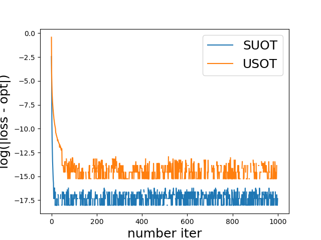
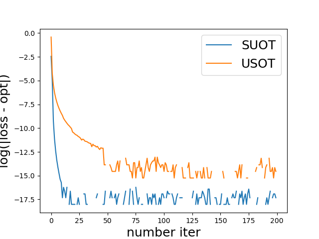
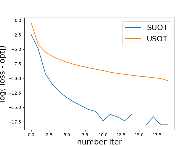
Figure 5: $|\text{{SUOT}}(\alpha,\beta)-\widehat{\text{{SUOT}}}_{t}|$ and $|\text{{USOT}}(\alpha,\beta)-\widehat{\text{{USOT}}}_{t}|$ against iteration $t$, where $\widehat{\text{{SUOT}}}_{t},\widehat{\text{{USOT}}}_{t}$ are the estimated SUOT, USOT using $t$ FW iterations. Plots are in log-scale. All figures are issued from the same run, but zoomed on a subset of first iterations: (left) 1000 iterations of FW, (middle) 200 iterations, (right) 20 iterations.

Appendix C Additional details on Section 5

C.1 Document classification: Technical details and additional results

C.1.1 Datasets

Table 2: Dataset characteristics.

	BBCSport	Movies	Goodreads genre	Goodreads like
Doc	737	2000	1003	1003
Train	517	1500	752	752
Test	220	500	251	251
Classes	5	2	8	2
Mean words by doc	$116\pm 54$	$182\pm 65$	$1491\pm 538$	$1491\pm 538$
Median words by doc	104	175	1518	1518
Max words by doc	469	577	3499	3499

We sum up the statistics of the different datasets in Table 2.

BBCSport.

The BBCSport dataset contains articles between 2004 and 2005, and is composed of 5 classes. We average over the 5 same train/test split of [44]. The dataset can be found in https://github.com/mkusner/wmd/tree/master.

Movie Reviews.

The movie reviews dataset is composed of 1000 positive and 1000 negative reviews. We take five different random 75/25 train/test split. The data can be found in http://www.cs.cornell.edu/people/pabo/movie-review-data/.

Goodreads.

This dataset, proposed in [47], and which can be found at https://ritual.uh.edu/multi_task_book_success_2017/, is composed of 1003 books from 8 genres. A first possible classification task is to predict the genre. A second task is to predict the likability, which is a binary task where a book is said to have success if it has an average rating $\geq 3.5$ on the website Goodreads (https://www.goodreads.com). The five train/test split are randomly drawn with 75/25 proportions.

C.1.2 Technical Details

All documents are embedded with the Word2Vec model [45] in dimension $d=300$. The embedding can be found in https://drive.google.com/file/d/0B7XkCwpI5KDYNlNUTTlSS21pQmM/view?resourcekey=0-wjGZdNAUop6WykTtMip30g.

In this experiment, we report the results averaged over 5 random train/test split. For discrepancies which are approximated using random projections, we additionally average the results over 3 different computations, and we report this standard deviation in Figure 3. Furthermore, we always use 500 projections to approximate the sliced discrepancies. For Frank-Wolfe based methods, we use 10 iterations, which we found to be enough to have a good accuracy. We added an ablation of these two hyperparameters in Figure 7. We report the results obtained with the best $\rho$ for USOT and SUOT computed among a grid $\rho\in\{10^{-4},5\cdot 10^{-4},10^{-3},5\cdot 10^{-3},10^{-2},10^{-1},1\}$. For USOT, the best $\rho$ is consistently $5\cdot 10^{-3}$ for the Movies and Goodreads datasets, and $5\cdot 10^{-4}$ for the BBCSport dataset. For SUOT, the best $\rho$ obtained was $0.01$ for the BBCSport dataset, $1.0$ for the movies dataset and $0.5$ for the goodreads dataset. For UOT, we used $\rho=1.0$ on the BBCSport dataset. For the movies dataset, the best $\rho$ obtained on a subset was 50, but it took an unreasonable amount of time to run on the full dataset as the runtime increases with $\rho$ (see [48, Figure 3]). On the goodreads dataset, it took too much memory on the GPU. For Sinkhorn UOT, we used $\varepsilon=0.001$ and $\rho=0.1$ on the BBCSport and Goodreads datasets, and $\varepsilon=0.01$ on the Movies dataset. For each method, the number of neighbors used for the k-NN method is obtained via cross-validation.

C.1.3 Additional experiments

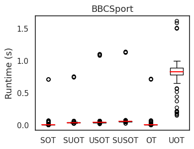
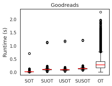
Figure 6: Runtime on the BBCSport dataset (left) and on the Goodreads dataset (right).

Runtime.

We report in Figure 6 the runtime of computing the different discrepancies between each pair of documents. On the BBCSport dataset, the documents have in average 116 words, thus the main bottleneck is the projection step for sliced OT methods. Hence, we observe that OT runs slightly faster than SOT and the sliced unbalanced counterparts. Goodreads is a dataset with larger documents, with on average 1491 words by document. Therefore, as OT scales cubically with the number of samples, we observe here that all sliced methods run faster than OT, which confirms that sliced methods scale better w.r.t. the number of samples. In this setting, we were not able to compute UOT with the POT implementation in a reasonable time. Computations have been performed with a NVIDIA A100 GPU.

Ablations.

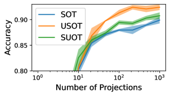
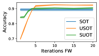
Figure 7: Ablation on BBCSport of the number of projections (left) and of the number of Frank-Wolfe iterations (right).

We plot in Figure 7 accuracy as a function of the number of projections and the number of iterations of the Frank-Wolfe algorithm. We averaged the accuracy obtained with the same setting described in Section C.1.2, with varying number of projections $K\in\{4,10,21,46,100,215,464,1000\}$ and number of FW iterations $F\in\{1,2,3,4,5,10,15,20\}$. Regarding the hyperparameter $\rho$, we selected the one returning the best accuracy, i.e. $\rho=5\cdot 10^{-4}$ for USOT and $\rho=10^{-2}$ for SUOT.

C.2 Unbalanced sliced Wasserstein barycenters

We define below the formulation of the USOT barycenter which was used in the experiments of Figure 4 to average predictions of geophysical data. We then detail how we computed it.

Definition 4.

Consider a set of measures $(\alpha_{1},\ldots,\alpha_{B})\in\mathcal{M}_{+}(\mathbb{R}^{d})^{B}$, and a set of non-negative coefficients $(\omega_{1},\ldots,\omega_{B})\geq 0$ such that $\sum_{b=1}^{B}\omega_{b}=1$. We define the barycenter problem (in the KL setting) as

$$\mathcal{B}((\alpha_{b})_{b},(\omega_{b})_{b}) \triangleq\inf_{\beta\in\mathcal{P}(\mathbb{R}^{d})}\sum_{b=1}^{B}\omega_{b}\text{{USOT}}(\alpha_{b},\beta),$$ (96)

$$=\inf_{\beta\in\mathcal{P}(\mathbb{R}^{d})}\sum_{b=1}^{B}\inf_{(\pi_{b,1},\pi_{b,2})}\text{{SOT}}(\pi_{b,1},\pi_{b,2})+\rho_{1}\text{{KL}}(\pi_{b,1}|\alpha_{b})+\rho_{2}\text{{KL}}(\pi_{b,2}|\beta),$$ (97)

where $\mathcal{P}(\mathbb{R}^{d})$ denotes the set of probability measures.

To compute the barycenter, we aggregate several building blocks. First, since we consider that the barycenter $\beta\in\mathcal{P}(\mathbb{R}^{d})$ is a probability, we perform mirror descent as in [65, 66]. More precisely, we use a Nesterov accelerated version of mirror descent. We also tried projected gradient descent, but it did not yield consistent outputs (due to convergence speed [65]). Second, we use a Stochastic-USOT version (see Section 4), i.e. we sample new projections at each iteration of the barycenter update (but not a each iteration of the FW subroutines in Algorithm 2). This procedure is described in Algorithm 8.

Algorithm 8 – $\texttt{Barycenter}((\alpha_{b})_{b},(\omega_{b})_{b},\rho_{1},\rho_{2},lr)$

Input: measures $(\alpha_{b})_{b}$, weights $(\omega_{b})_{b}$, $\rho_{1}$, $\rho_{2}$, learning rate $lr$, FW iter $F$
Output: Optimal barycenter $\beta$ of Equation (96)

  $t\leftarrow 1$

  Init $(\beta,\tilde{\beta},\hat{\beta})$ as uniform distribution over a grid

  while not converged do do

     $\gamma\leftarrow\tfrac{2}{(t+1)}$,

     $\beta\rightarrow(1-\gamma)\hat{\beta}+\gamma\tilde{\beta}$

     Sample projections $(\theta_{k})_{k=1}^{K}$

     Compute $\mathcal{B}((\alpha_{b})_{b},(\omega_{b})_{b})$ by calling $\text{{USOT}}(\alpha_{b},\beta,F,(\theta_{k})_{k=1}^{K},\rho_{1},\rho_{2})$ in Algorithm 2 for each $b$

     Compute $g$ as the gradient of $\mathcal{B}((\alpha_{b})_{b},(\omega_{b})_{b})$ w.r.t. variable $\beta$

     $\tilde{\beta}\leftarrow\exp(-lr\times\gamma^{-1}\times g)\beta$

     $\tilde{\beta}\leftarrow\tilde{\beta}/m(\tilde{\beta})$

     $\hat{\beta}\leftarrow(1-\gamma)\hat{\beta}+\gamma\tilde{\beta}$

     $t\leftarrow t+1$

  end while

We illustrate this algorithm with several examples of interpolation in Figure 8. We propose to compute an interpolation between two measures located on a fixed grid of size $200\times 200$ with different values of $\rho_{i}$ in $\text{D}_{\varphi_{i}}=\rho_{i}\text{{KL}}$. For illustration purposes, we construct the source distribution as a mixture of two Gaussians with a small and a larger mode, and the target distribution as a single Gaussian. Those distributions are normalized over the grid such that both total norms are equal to one (which is not required by our unbalanced sliced variants but grants more interpretability and possible comparisons with SOT). Figure 8(a) shows the result of the interpolation at three timestamps ($t=0.25,\;0.5$ and $0.75$) of a SOT interpolation (within this setting, $\omega_{1}=1-t$ and $\omega_{2}=t$). As expected, the two modes of the source distribution are transported over the target one. We verify in Figure 8(b) that for a large value of $\rho_{1}=\rho_{2}=100$, the USOT interpolation behaves similarly as SOT, as expected from the theory. When $\rho_{1}=\rho_{2}=0.01$, the smaller mode is not moved during the interpolation, whereas the larger one is stretched toward the target (Figure 8(c)). Finally, in Figure 8(d), an asymmetric configuration of $\rho_{1}=0.01$ and $\rho_{2}=100$ allows to get an interpolation when only the big mode of the source distribution is displaced toward the target. In all those cases, the mirror-descent algorithm 8 is run for $500$ iterations. Even for a large grid of $200\times 200$, those different results are obtained in a $2-3$ minutes on a commodity GPU, while the OT or UOT barycenters are untractable with a limited computational budget.

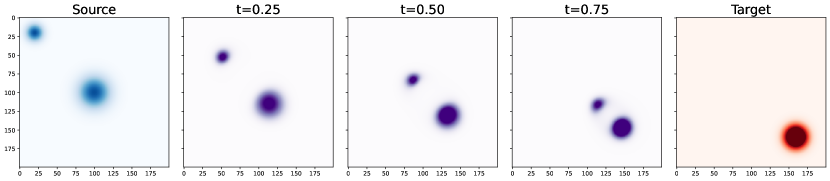
(a) SOT barycenters

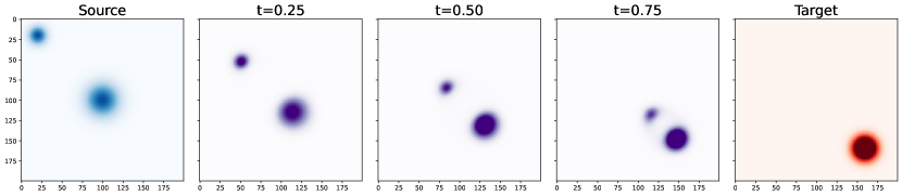
(b) USOT barycenters with $\rho_{1}=\rho_{2}=100$

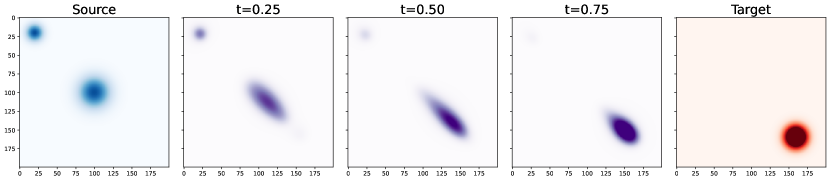
(c) USOT barycenters with $\rho_{1}=\rho_{2}=0.01$

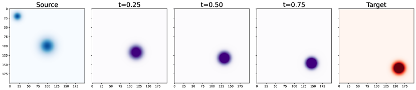
(d) USOT barycenters with $\rho_{1}=0.01$ and $\rho_{2}=100$

Figure 8: Interpolation with USOT as a barycenter computation. We compare different interpolations using SOT or USOT with different settings for the $\rho$ values

References

- [1] Martin Arjovsky, Soumith Chintala, and Léon Bottou. Wasserstein generative adversarial networks. In International conference on machine learning, pages 214–223. PMLR, 2017.
- [2] Valentin De Bortoli, James Thornton, Jeremy Heng, and Arnaud Doucet. Diffusion schrödinger bridge with applications to score-based generative modeling. Advances in Neural Information Processing Systems, 34:17695–17709, 2021.
- [3] Geoffrey Schiebinger, Jian Shu, Marcin Tabaka, Brian Cleary, Vidya Subramanian, Aryeh Solomon, Joshua Gould, Siyan Liu, Stacie Lin, Peter Berube, et al. Optimal-transport analysis of single-cell gene expression identifies developmental trajectories in reprogramming. Cell, 176(4):928–943, 2019.
- [4] Matthias Liero, Alexander Mielke, and Giuseppe Savaré. Optimal entropy-transport problems and a new hellinger–kantorovich distance between positive measures. Inventiones mathematicae, 211(3):969–1117, 2018.
- [5] Stanislav Kondratyev, Léonard Monsaingeon, and Dmitry Vorotnikov. A fitness-driven cross-diffusion system from population dynamics as a gradient flow. Journal of Differential Equations, 261(5):2784–2808, 2016.
- [6] Lenaic Chizat, Gabriel Peyré, Bernhard Schmitzer, and François-Xavier Vialard. Unbalanced optimal transport: Dynamic and kantorovich formulations. Journal of Functional Analysis, 274(11):3090–3123, 2018.
- [7] Lenaic Chizat and Francis Bach. On the global convergence of gradient descent for over-parameterized models using optimal transport. Advances in neural information processing systems, 31, 2018.
- [8] Grant Rotskoff, Samy Jelassi, Joan Bruna, and Eric Vanden-Eijnden. Global convergence of neuron birth-death dynamics. arXiv preprint arXiv:1902.01843, 2019.
- [9] Pinar Demetci, Rebecca Santorella, Manav Chakravarthy, Bjorn Sandstede, and Ritambhara Singh. Scotv2: Single-cell multiomic alignment with disproportionate cell-type representation. Journal of Computational Biology, 29(11):1213–1228, 2022.
- [10] Kilian Fatras, Thibault Sejourne, Rémi Flamary, and Nicolas Courty. Unbalanced minibatch optimal transport; applications to domain adaptation. In Marina Meila and Tong Zhang, editors, Proceedings of the 38th International Conference on Machine Learning, volume 139 of Proceedings of Machine Learning Research, pages 3186–3197. PMLR, 18–24 Jul 2021.
- [11] Thibault Séjourné, Gabriel Peyré, and François-Xavier Vialard. Unbalanced optimal transport, from theory to numerics. arXiv preprint arXiv:2211.08775, 2022.
- [12] Richard Mansfield Dudley. The speed of mean glivenko-cantelli convergence. The Annals of Mathematical Statistics, 40(1):40–50, 1969.
- [13] Marco Cuturi. Sinkhorn distances: Lightspeed computation of optimal transport. Advances in neural information processing systems, 26, 2013.
- [14] Kilian Fatras, Younes Zine, Rémi Flamary, Remi Gribonval, and Nicolas Courty. Learning with minibatch wasserstein : asymptotic and gradient properties. In Silvia Chiappa and Roberto Calandra, editors, Proceedings of the Twenty Third International Conference on Artificial Intelligence and Statistics, volume 108 of Proceedings of Machine Learning Research, pages 2131–2141, Online, 26–28 Aug 2020. PMLR.
- [15] Johann Radon. 1.1 über die bestimmung von funktionen durch ihre integralwerte längs gewisser mannigfaltigkeiten. Classic papers in modern diagnostic radiology, 5(21):124, 2005.
- [16] Nicolas Bonneel, Julien Rabin, Gabriel Peyré, and Hanspeter Pfister. Sliced and radon wasserstein barycenters of measures. Journal of Mathematical Imaging and Vision, 51:22–45, 2015.
- [17] Gabriel Peyré, Marco Cuturi, et al. Computational optimal transport: With applications to data science. Foundations and Trends® in Machine Learning, 11(5-6):355–607, 2019.
- [18] Erhan Bayraktar and Gaoyue Guo. Strong equivalence between metrics of Wasserstein type. Electronic Communications in Probability, 26(none):1 – 13, 2021.
- [19] Kimia Nadjahi, Alain Durmus, Lénaïc Chizat, Soheil Kolouri, Shahin Shahrampour, and Umut Simsekli. Statistical and topological properties of sliced probability divergences. Advances in Neural Information Processing Systems, 33:20802–20812, 2020.
- [20] Ziv Goldfeld and Kristjan Greenewald. Sliced mutual information: A scalable measure of statistical dependence. In M. Ranzato, A. Beygelzimer, Y. Dauphin, P.S. Liang, and J. Wortman Vaughan, editors, Advances in Neural Information Processing Systems, volume 34, pages 17567–17578. Curran Associates, Inc., 2021.
- [21] Soheil Kolouri, Kimia Nadjahi, Umut Simsekli, Roland Badeau, and Gustavo Rohde. Generalized sliced wasserstein distances. Advances in neural information processing systems, 32, 2019.
- [22] Ishan Deshpande, Yuan-Ting Hu, Ruoyu Sun, Ayis Pyrros, Nasir Siddiqui, Sanmi Koyejo, Zhizhen Zhao, David Forsyth, and Alexander G Schwing. Max-sliced wasserstein distance and its use for gans. In Proceedings of the IEEE/CVF Conference on Computer Vision and Pattern Recognition, pages 10648–10656, 2019.
- [23] Khai Nguyen, Nhat Ho, Tung Pham, and Hung Bui. Distributional sliced-wasserstein and applications to generative modeling. arXiv preprint arXiv:2002.07367, 2020.
- [24] Ruben Ohana, Kimia Nadjahi, Alain Rakotomamonjy, and Liva Ralaivola. Shedding a pac-bayesian light on adaptive sliced-wasserstein distances. In Proceedings of the 40th International Conference on Machine Learning, 2023.
- [25] Clément Bonet, Paul Berg, Nicolas Courty, François Septier, Lucas Drumetz, and Minh-Tan Pham. Spherical sliced-wasserstein. In The Eleventh International Conference on Learning Representations, 2023.
- [26] Clément Bonet, Laetitia Chapel, Lucas Drumetz, and Nicolas Courty. Hyperbolic sliced-wasserstein via geodesic and horospherical projections. arXiv preprint arXiv:2211.10066, 2022.
- [27] Clément Bonet, Benoît Malézieux, Alain Rakotomamonjy, Lucas Drumetz, Thomas Moreau, Matthieu Kowalski, and Nicolas Courty. Sliced-wasserstein on symmetric positive definite matrices for m/eeg signals. In Proceedings of the 40th International Conference on Machine Learning, 2023.
- [28] Nicolas Bonneel and David Coeurjolly. Spot: sliced partial optimal transport. ACM Transactions on Graphics (TOG), 38(4):1–13, 2019.
- [29] Yikun Bai, Bernard Schmitzer, Mathew Thorpe, and Soheil Kolouri. Sliced optimal partial transport. arXiv preprint arXiv:2212.08049, 2022.
- [30] Ryoma Sato, Makoto Yamada, and Hisashi Kashima. Fast unbalanced optimal transport on a tree. Advances in neural information processing systems, 33:19039–19051, 2020.
- [31] Thibault Séjourné, François-Xavier Vialard, and Gabriel Peyré. Faster unbalanced optimal transport: Translation invariant sinkhorn and 1-d frank-wolfe. In International Conference on Artificial Intelligence and Statistics, pages 4995–5021. PMLR, 2022.
- [32] Marguerite Frank and Philip Wolfe. An algorithm for quadratic programming. Naval research logistics quarterly, 3(1-2):95–110, 1956.
- [33] Lenaic Chizat, Gabriel Peyré, Bernhard Schmitzer, and François-Xavier Vialard. An interpolating distance between optimal transport and fisher–rao metrics. Foundations of Computational Mathematics, 18:1–44, 2018.
- [34] Khiem Pham, Khang Le, Nhat Ho, Tung Pham, and Hung Bui. On unbalanced optimal transport: An analysis of Sinkhorn algorithm. In Hal Daumé III and Aarti Singh, editors, Proceedings of the 37th International Conference on Machine Learning, volume 119 of Proceedings of Machine Learning Research, pages 7673–7682. PMLR, 13–18 Jul 2020.
- [35] Julien Rabin, Gabriel Peyré, Julie Delon, and Marc Bernot. Wasserstein barycenter and its application to texture mixing. In Scale Space and Variational Methods in Computer Vision: Third International Conference, SSVM 2011, Ein-Gedi, Israel, May 29–June 2, 2011, Revised Selected Papers 3, pages 435–446. Springer, 2012.
- [36] Luigi Ambrosio, Nicola Gigli, and Giuseppe Savaré. Gradient flows: in metric spaces and in the space of probability measures. Springer Science & Business Media, 2005.
- [37] Clément Bonet, Nicolas Courty, François Septier, and Lucas Drumetz. Efficient gradient flows in sliced-wasserstein space. Transactions on Machine Learning Research, 2022.
- [38] Jules Candau-Tilh. Wasserstein and sliced-wasserstein distances. Master’s thesis, Université Pierre et Marie Curie, 2020.
- [39] Adrien Vacher and François-Xavier Vialard. Stability of semi-dual unbalanced optimal transport: fast statistical rates and convergent algorithm. 2022.
- [40] Sloan Nietert, Ziv Goldfeld, and Rachel Cummings. Outlier-robust optimal transport: Duality, structure, and statistical analysis. In Proceedings of The 25th International Conference on Artificial Intelligence and Statistics. PMLR, 2022.
- [41] Adam Paszke, Sam Gross, Francisco Massa, Adam Lerer, James Bradbury, Gregory Chanan, Trevor Killeen, Zeming Lin, Natalia Gimelshein, Luca Antiga, et al. Pytorch: An imperative style, high-performance deep learning library. Advances in neural information processing systems, 32, 2019.
- [42] Simon Lacoste-Julien and Martin Jaggi. On the global linear convergence of frank-wolfe optimization variants. Advances in neural information processing systems, 28, 2015.
- [43] Yoshihiro Nagano, Shoichiro Yamaguchi, Yasuhiro Fujita, and Masanori Koyama. A wrapped normal distribution on hyperbolic space for gradient-based learning. In International Conference on Machine Learning, pages 4693–4702. PMLR, 2019.
- [44] Matt Kusner, Yu Sun, Nicholas Kolkin, and Kilian Weinberger. From word embeddings to document distances. In International conference on machine learning, pages 957–966. PMLR, 2015.
- [45] Tomas Mikolov, Ilya Sutskever, Kai Chen, Greg S Corrado, and Jeff Dean. Distributed representations of words and phrases and their compositionality. Advances in neural information processing systems, 26, 2013.
- [46] Bo Pang, Lillian Lee, and Shivakumar Vaithyanathan. Thumbs up? sentiment classification using machine learning techniques. In Proceedings of EMNLP, pages 79–86, 2002.
- [47] Suraj Maharjan, John Arevalo, Manuel Montes, Fabio A González, and Thamar Solorio. A multi-task approach to predict likability of books. In Proceedings of the 15th Conference of the European Chapter of the Association for Computational Linguistics: Volume 1, Long Papers, pages 1217–1227, 2017.
- [48] Laetitia Chapel, Rémi Flamary, Haoran Wu, Cédric Févotte, and Gilles Gasso. Unbalanced optimal transport through non-negative penalized linear regression. Advances in Neural Information Processing Systems, 34:23270–23282, 2021.
- [49] Rémi Flamary, Nicolas Courty, Alexandre Gramfort, Mokhtar Z Alaya, Aurélie Boisbunon, Stanislas Chambon, Laetitia Chapel, Adrien Corenflos, Kilian Fatras, Nemo Fournier, et al. Pot: Python optimal transport. The Journal of Machine Learning Research, 22(1):3571–3578, 2021.
- [50] Khang Le, Huy Nguyen, Quang M Nguyen, Tung Pham, Hung Bui, and Nhat Ho. On robust optimal transport: Computational complexity and barycenter computation. In M. Ranzato, A. Beygelzimer, Y. Dauphin, P.S. Liang, and J. Wortman Vaughan, editors, Advances in Neural Information Processing Systems, volume 34, pages 21947–21959, 2021.
- [51] Marco Cuturi and Arnaud Doucet. Fast computation of wasserstein barycenters. In Eric P. Xing and Tony Jebara, editors, Proceedings of the 31st International Conference on Machine Learning, volume 32 of Proceedings of Machine Learning Research, pages 685–693, Bejing, China, 22–24 Jun 2014. PMLR.
- [52] Benjamin M Sanderson, Reto Knutti, and Peter Caldwell. A representative democracy to reduce interdependency in a multimodel ensemble. Journal of Climate, 28(13):5171–5194, 2015.
- [53] Soulivanh Thao, Mats Garvik, Gregoire Mariethoz, and Mathieu Vrac. Combining global climate models using graph cuts. Climate Dynamics, 59:2345–2361, 2022.
- [54] Prabhat, K. Kashinath, M. Mudigonda, S. Kim, L. Kapp-Schwoerer, A. Graubner, E. Karaismailoglu, L. von Kleist, T. Kurth, A. Greiner, A. Mahesh, K. Yang, C. Lewis, J. Chen, A. Lou, S. Chandran, B. Toms, W. Chapman, K. Dagon, C. A. Shields, T. O’Brien, M. Wehner, and W. Collins. Climatenet: an expert-labeled open dataset and deep learning architecture for enabling high-precision analyses of extreme weather. Geoscientific Model Development, 14(1):107–124, 2021.
- [55] Soheil Kolouri, Yang Zou, and Gustavo K Rohde. Sliced wasserstein kernels for probability distributions. In Proceedings of the IEEE Conference on Computer Vision and Pattern Recognition, pages 5258–5267, 2016.
- [56] Mathieu Carriere, Marco Cuturi, and Steve Oudot. Sliced wasserstein kernel for persistence diagrams. In International conference on machine learning, pages 664–673. PMLR, 2017.
- [57] Filippo Santambrogio. Optimal transport for applied mathematicians. Birkäuser, NY, 55(58-63):94, 2015.
- [58] Vladimir Igorevich Bogachev and Maria Aparecida Soares Ruas. Measure theory, volume 1. Springer, 2007.
- [59] Nicolas Bonnotte. Unidimensional and evolution methods for optimal transportation. PhD thesis, Université Paris Sud-Paris XI; Scuola normale superiore (Pise, Italie), 2013.
- [60] Aude Genevay, Lénaic Chizat, Francis Bach, Marco Cuturi, and Gabriel Peyré. Sample complexity of sinkhorn divergences. In The 22nd international conference on artificial intelligence and statistics, pages 1574–1583. PMLR, 2019.
- [61] Benedetto Piccoli and Francesco Rossi. Generalized wasserstein distance and its application to transport equations with source. Archive for Rational Mechanics and Analysis, 211:335–358, 2014.
- [62] Thibault Séjourné, Jean Feydy, François-Xavier Vialard, Alain Trouvé, and Gabriel Peyré. Sinkhorn divergences for unbalanced optimal transport. arXiv preprint arXiv:1910.12958, 2019.
- [63] Stephen Simons. Minimax and monotonicity. Springer, 2006.
- [64] Jiaqi Xi and Jonathan Niles-Weed. Distributional convergence of the sliced wasserstein process. arXiv preprint arXiv:2206.00156, 2022.
- [65] Amir Beck and Marc Teboulle. Mirror descent and nonlinear projected subgradient methods for convex optimization. Operations Research Letters, 31(3):167–175, 2003.
- [66] Marco Cuturi and Arnaud Doucet. Fast computation of wasserstein barycenters. In International conference on machine learning, pages 685–693. PMLR, 2014.