$L_{q}$ norms and Mahler measure of Fekete polynomials

Abstract.

We show that the distribution of the values of Fekete polynomials $F_{p}$ on the unit circle is governed, as $p\to\infty$, by an explicit limiting (non-Gaussian) random point process.
This allows us to prove that the Mahler measure of $F_{p}$ satisfies

$$M_{0}(F_{p})\sim k_{0}\sqrt{p},$$

as $p\to\infty$ where $k_{0}=0.74083\dots,$ thus solving an old open problem.
Further, we obtain an asymptotic formula for all moments $\|F_{p}\|_{q}$ with $0<q<\infty,$ resolving another open problem and improving previous results of Günther and Schmidt (who treated the case $q=2k,$ $k\in\mathbb{N}$).

1. Introduction

Erdős and Littlewood explored various extremal problems concerning polynomials with coefficients $\pm 1$ (see in particular Littlewood’s delightful monograph [42]) which spurred intensive research throughout the past seventy years. Here, we mention recent breakthrough results solving Littlewood’s conjecture on the existence of flat polynomials [2, 4, 15, 37] (see also [9, 11, 26, 45, 47, 48] and the references therein for a historical account of such problems and the link with Barker sequences and several related engineering problems).
Among various classes of Littlewood polynomials two specific examples attracted particular attention: the Fekete and the Rudin-Shapiro polynomials [22, 23, 35, 49, 50]. For a given prime $p,$ we recall that the corresponding Fekete polynomial is defined by

$$F_{p}(z):=\sum_{n=1}^{p-1}\left(\frac{n}{p}\right)z^{n},$$

where $\left(\frac{\cdot}{p}\right)$ is the Legendre symbol modulo $p$. The family of Fekete polynomials appears frequently in the context of both number theoretic and analytic problems and has been extensively studied for over a century, see [1], [3], [5], [10], [12], [13], [17], [27], [30], [31], [34], [35], [36], [44] for some of the results. Dirichlet was perhaps the first to discover the identity

$$L\left(s,\left(\frac{\cdot}{p}\right)\right)\Gamma(s)=\int_{0}^{1}\frac{(-\log x)^{s-1}}{x}\frac{F_{p}(x)}{1-x^{p}}dx,$$

where $L(s,\chi)$ is the Dirichlet $L$-function associated to a Dirichlet character $\chi$ modulo $p$. Consequently, if $F_{p}$ has no zeros for $0<x<1,$ then $L\left(s,\left(\frac{\cdot}{p}\right)\right)>0$ for all $0<s<1,$ which in turn refute the existence of a putative Siegel zero. The positivity of $L(s,\chi_{d})$ however (where $\chi_{d}$ is the Kronecker symbol associated to a fundamental discriminant $d$), is only known for a positive proportion of fundamental discriminants $d$ by the work of Conrey and Soundararajan [19].

1.1. The Mahler measure of Fekete polynomials

A classical quantity related to the distribution of complex zeros of an algebraic polynomial $P\in\mathbb{C}[x]$ is the Mahler measure of $P$ given by

$$M_{0}(P):=\exp\left(\int_{0}^{1}\log|P(e(t))|dt\right),$$

where $e(t):=e^{2\pi it}$. The problem of determining an asymptotic formula for the Mahler measure of Fekete polynomials has attracted considerable attention. Littlewood [41] was the first to prove a general upper bound for the Mahler measure of Littlewood polynomials, from which one has $M_{0}(F_{p})\leq(1-\varepsilon_{0})\sqrt{p-1}$ for some small fixed $\varepsilon_{0}>0.$ Using subharmonic methods, Erdélyi and Lubinskii [25] established the lower bound $M_{0}(F_{p})\geq(\frac{1}{2}-\varepsilon)\sqrt{p},$ which has since been improved in [21] to $M_{0}(F_{p})\geq(\frac{1}{2}+c_{1})\sqrt{p},$ for some small value of $c_{1}>0.$ In [22] (see also recent survey [24]), Erdélyi writes the following about the problem of finding an asymptotic formula for $M_{0}(F_{p})$:

“…this problem seems to be beyond reach at the moment. Not even a (published or unpublished) conjecture about the asymptotic seems to be known.”

Our first result resolves this problem.

Theorem 1.1.

Let ${G}_{\mathbb{X}}$ be the random process on $C[0,1]$ defined by

(1.1) $$G_{\mathbb{X}}(t):=\sum_{m\in\mathbb{Z}}\frac{e(t)-1}{2\pi i(m-t)}\mathbb{X}(m),\hskip 5.69054ptt\in[0,1]$$

where $\{\mathbb{X}(m)\}_{m\in\mathbb{Z}}$ are I. I. D. random variables taking the values $\pm 1$ with equal probability $1/2$. Then we have

$$\lim_{p\to\infty}\frac{M_{0}(F_{p})}{\sqrt{p}}=k_{0}:=\int_{0}^{1}\mathbb{E}\left(\log|{G}_{\mathbb{X}}(t)|\right)dt,$$

where the constant $k_{0}=0.74083\dots$ is effectively computable (see Remark 6.4 for details).

Remark 1.2.

There are a series of related results concerning the average behaviour of the Mahler measure for a typical Littlewood polynomial (with coefficients $\pm 1$). Here, a general result due to Choi and Erdélyi [16], relying on a deep work of Konyagin and Schlag [38], states that on average

(1.2) $$\lim_{n\to\infty}\frac{1}{2^{n+1}}\sum_{f\in\mathcal{L}_{n}}\frac{M_{0}(f)}{\sqrt{n}}=e^{-\gamma/2}=0.749306\dots,$$

where $\mathcal{L}_{n}$ denotes the set of polynomials of degree $n$ with $\pm 1$ coefficients. Our constant $k_{0}$ differs from the one in (1.2) and from the previous examples in the literature. On a related note, relying on a beautiful result of Rodgers [49], Erdélyi [22] recently proved Saffari’s conjecture about the asymptotic behavior for the Mahler measure of the Rudin-Shapiro polynomials $P_{k}(z)$ (of degree $2^{k}-1$), which states that

$$\lim_{k\to\infty}\frac{M_{0}(P_{k})}{\sqrt{2^{k+1}}}=e^{-1/2}.$$

1.2. $L_{q}$ norms of Fekete polynomials

A well-known result of Borwein and Lockhart [14] states that for every $0<q<\infty,$

$$\lim_{n\to\infty}\frac{1}{2^{n+1}}\sum_{f\in\mathcal{L}_{n}}\frac{M_{q}(f)}{\sqrt{n}}=\Gamma\left(1+\frac{q}{2}\right)^{1/q},$$

where

$$M_{q}(P):=\left(\int_{0}^{1}|P(e(t))|^{q}dt\right)^{1/q}.$$

In the case of Fekete polynomials, the analogous problem has been extensively studied. Interestingly, Borwein and Choi [10] found the exact expressions for $||F_{p}||_{4}^{4}$ in terms of the class number of $\mathbb{Q}[\sqrt{-p}].$ Erdélyi [20] determined the exact order of the growth ($\asymp\sqrt{p}$) of $M_{q}(F_{p})$ for every $q>0.$ These investigations culminated in the work of Günther and Schmidt [28], who showed that for every integer $k\geq 1$ we have

$$\lim_{p\to\infty}\frac{M_{2k}(F_{p})}{\sqrt{p}}=(\ell_{2k})^{1/2k},$$

where the constant $\ell_{2k}$ is given via a series of rather complicated recursive combinatorial identities (Theorem 2.1 in [28]). Our next corollary recovers their result and extends it to all values $q>0$ via a different method.

Corollary 1.3.

Let ${G}_{\mathbb{X}}(t)$ be the random process defined in (1.1). Then for any $0<q<\infty,$ we have

$$\lim_{p\to\infty}\frac{M_{q}(F_{p})}{\sqrt{p}}=k_{q}:=\left(\int_{0}^{1}\mathbb{E}(|G_{\mathbb{X}}(t)|^{q})dt\right)^{1/q}.$$

Remark 1.4.

In the case $q=\infty,$ a beautiful result of Montgomery [44] shows that

$$\sqrt{p}\log\log p\ll M_{\infty}(F_{p})=\max_{|z|=1}|F_{p}(z)|\ll\sqrt{p}\log p,$$

but the exact order of the growth is still unknown.

1.3. Distributional result.

Establishing appealing conjectures of Montgomery and Saffari, Rodgers [49] recently proved a distributional result for the appropriately normalized family of the Rudin-Shapiro polynomials $P_{k}(z)$, showing that one has convergence to the uniform distribution on the unit disc $\{|z|\leq 1\}$ in this case. More precisely, one has

(1.3) $$\lim_{k\to\infty}\text{m}\left(t\in[0,1]:\frac{P_{k}(e(t))}{\sqrt{2^{k+1}}}\in U\right)=\frac{1}{\pi}|U|,$$

for any rectangle $U\subset\mathbb{C}$, where m is the standard Lebesgue measure, and $|U|$ is the area of $U$. Subsequently, Erdélyi [23] used (1.3) to show that a negligible proportion of the zeros of Rudin-Shapiro polynomials lie on the unit circle. This is in a strong contrast with a rather surprising result of Conrey, Granville, Poonen and Soundararajan [18], who showed that there exists a constant $1/2<c<1$ such that

$$\{z:|z|=1\ and\ F_{p}(z)=0\}\sim cp,$$

with $0.500668<c<0.500813.$ Our next theorem provides an analogue of the Montgomery-Saffari conjecture for Fekete polynomials.

Theorem 1.5.

Let $U\subset\mathbb{C}$ be a rectangle with sides parallel to the coordinate axes. Then we have

$$\lim_{p\rightarrow\infty}\text{m}\left(t\in[0,1]:\frac{F_{p}(e(t))}{F_{p}(\xi_{p})}\in U\right)=\mathbb{P}(G_{\mathbb{X}}(\theta)\in U),$$

where $\theta$ is a random variable uniformly distributed on $[0,1]$.

We refer our interested reader to the plot above for the visualisation of the random process $G_{\mathbb{X}}.$

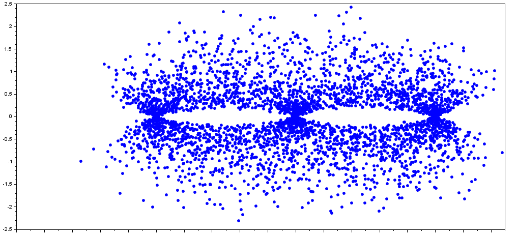
Figure 1. Realization of $G_{\mathbb{X}}(t),t\in(0,1)$

We now describe yet another relation of our results to the classical problem on the distribution of random trigonometric polynomials. A seminal result of Salem and Zygmund [51], shows that if the coefficients $a_{k}$ are independent identically distributed random variables taking values $\pm 1$ with probability $1/2$ each, then almost surely

$$\frac{1}{\sqrt{N}}\sum_{k\leq N}a_{k}e(k\theta)\xrightarrow{a.s.}\mathcal{CN}(0,1),$$

where the right hand side denotes a standard complex Gaussian distribution. In the case of sequences $a_{n}$ possessing some multiplicative properties, the situation is more subtle and often leads to various arithmetic consequences. See for example the work of Hughes and Rudnick [32] on lattice points in annuli. Another example is a recent result of Benatar, Nishry and Rodgers [6], which shows convergence to the Gaussian distribution when $a_{n}$ are random (Rademacher or Steinhaus) multiplicative functions.
Upon applying Fourier inversion, the distribution of a normalized trigonometric polynomial

(1.4) $$\frac{1}{\sqrt{H}}\sum_{k\leq H}\left(\frac{k}{p}\right)e(k\theta),$$

for various ranges of $H$ is essentially equivalent to the statistical behaviour of short character sums

$${\frac{1}{\sqrt{H}}\sum_{x\leq n\leq x+H}\left(\frac{n}{p}\right)},$$

for a randomly chosen interval $[x,x+H]$ with $x\in\{0,1,\dots,p-1\}$. It follows from a recent work of Harper [29] that for almost all primes $p$ the sum (1.4) converges to the standard Gaussian in the range $H\sim(\log p)^{A}$ (where $A\geq 1$ is a fixed constant) when $\theta\in[0,1]$ is selected uniformly at random. In contrast, Harper [29] shows the existence of a sequence of primes $p$ with $p\to\infty,$ where the corresponding sums in (1.4) do not satisfy the central limit theorem for this range of $H$.
It remains a deep mystery to understand the behaviour of (1.4) for different ranges of $1\leq H\leq p$ and our Theorem 1.5 shows that in the extreme case $H=p,$ the distribution of (1.4) is governed by the random process given by (1.1), and is in particular non-Gaussian.

2. Plan of attack

We now briefly outline our general strategy. We consider the auxiliary function

$$G_{p}(k,t):=\frac{F_{p}\left(e\left(\frac{k+t}{p}\right)\right)}{F_{p}(\zeta_{p})},$$

where $\zeta_{p}:=e(1/p)$. Note that

(2.1) $$F_{p}(\zeta_{p})=\sum_{n=1}^{p}\left(\frac{n}{p}\right)e(n/p)=\begin{cases}\sqrt{p},&\text{ if }p\equiv 1\pmod{4},\\ i\sqrt{p},&\text{ if }p\equiv 3\pmod{4}.\end{cases}$$

is the Gauss sum associated to the Legendre symbol modulo $p$.

The key starting point in our investigations is the identity borrowed from [18, Formulas $(2.2)$ and $(2.3)$] which implies that

$$G_{p}(k,t)=\sum_{|m|\leq(p-1)/2}\bigg{(}\frac{k-m}{p}\bigg{)}\frac{e(t)-1}{p(e(\frac{m-t}{p})-1)}.$$

Given $|m|\leq(p-1)/2,$ we now aim to exploit the “randomness” coming from the action of the shifts $\bigg{(}\frac{k-m}{p}\bigg{)}$ for various $0\leq k\leq p-1.$ To this end, we view $(G_{p}(k,t))_{t\in[0,1]}$ as a random process on the finite probability space $\mathbb{F}_{p}$ equipped with the uniform measure. Our goal is to prove the following result.

Theorem 2.1.

For any bounded continuous function $\varphi:C[0,1]\to\mathbb{C}$ we have

(2.2) $$\lim_{p\to\infty}\frac{1}{p}\sum_{k=0}^{p-1}\varphi\left(\frac{F_{p}\left(e\left(\frac{k+t}{p}\right)\right)}{F_{p}(\zeta_{p})}\right)=\mathbb{E}\varphi(G_{\mathbb{X}}),$$

where $G_{\mathbb{X}}$ is defined in (1.1).

In probabilistic terms, Theorem 2.1 is equivalent to the statement that the sequence of random processes $(G_{p}(k,t))_{t\in[0,1]}$ converges in law (in the space of continuous functions on $[0,1]$) to the process $(G_{\mathbb{X}}(t))_{t\in[0,1]}$. There are two main ingredients to prove this convergence in law. The first is proving the convergence of finite distributions, that is the convergence of finite moments, which will be established in Section 4.1. The second ingredient is to show that the sequence of random processes $(G_{p}(k,t))_{t\in[0,1]}$ is relatively compact, which is equivalent, by Prokhorov’s theorem, to verifying the “tightness” of these processes (this is the content of Section 4.2).

Now we can write the logarithmic Mahler measure of $F_{p}$ as follows

$$\log M_{0}(F_{p})=\int_{0}^{1}\log|F_{p}(e(t))|dt=\frac{1}{p}\sum_{k=0}^{p-1}\int_{0}^{1}\log\bigg{|}F_{p}\bigg{(}e\bigg{(}\frac{k+t}{p}\bigg{)}\bigg{)}\bigg{|}dt$$

$$=\log\sqrt{p}+\frac{1}{p}\sum_{k=0}^{p-1}\int_{0}^{1}\log|G_{p}(k,t)|dt,$$

since $|F_{p}(\zeta_{p})|=\sqrt{p}$. We note that the functional $\ell(\phi)=\int_{0}^{1}\log|\phi(t)|dt$ is not continuous on $C[0,1]$ and so we cannot apply Theorem 2.1 directly. We thus have to deal with the issues of uniform “log-integrability,” which is a classical topic in the theory of random and deterministic Fourier series and our treatment is inspired by the work of Nazarov, Nishry and Sodin [46]. Roughly speaking, to overcome this obstacle, we instead consider the regularized functional $\ell_{\epsilon}(\phi)=\int_{\varepsilon}^{1-\varepsilon}\log(|\phi(t)|)\mathbbm{1}_{|\phi(t)|\geq\varepsilon}dt,$ to which our Theorem 2.1 applies. We then show that uniformly for each function in our family, either $|\frac{G_{p,k}^{\prime}(t)}{e(t)-1}|\gg 1,$ or $|\frac{G_{p,k}^{\prime\prime}(t)}{e(t)-1}|\gg 1,$ which then allows us, after some technical work, to adequately control the logarithmic singularities on both random and deterministic sides.

3. Preparatory results

We begin with several simple observations concerning the random process.

Lemma 3.1.

The functions $t\rightarrow\Re G_{\mathbb{X}}(t)$ and $t\rightarrow\Im G_{\mathbb{X}}(t)$ are almost surely real-analytic on $[0,1]$.

Proof.

We only prove the result for $\Re G_{\mathbb{X}}(t)$ since the proof for $\Im G_{\mathbb{X}}(t)$ is similar. We write

$$\Re G_{\mathbb{X}}(t)=\Re\sum_{m\in\mathbb{Z}}\frac{e(t)-1}{2\pi i(m-t)}\mathbb{X}(m)=\sum_{|m|\geq 2}\frac{\sin(2\pi t)}{2\pi(m-t)}\mathbb{X}(m)+\sum_{m=-1,0,1}\frac{\sin(2\pi t)}{2\pi(m-t)}\mathbb{X}(m),$$

and observe that the second sum defines an analytic function over all realizations of $\mathbb{X}(-1),\mathbb{X}(0)$ and $\mathbb{X}(1).$ Since $\sin(2\pi t)$ is analytic it is enough to show that the random function

$$G_{\mathbb{X},2}(t)=\sum_{|m|\geq 2}\frac{\mathbb{X}(m)}{m-t}$$

is almost surely analytic. We notice that

$$G^{\prime}_{\mathbb{X},2}(t)=\sum_{|m|\geq 2}\frac{\mathbb{X}(m)}{(m-t)^{2}}$$

is absolutely convergent over all realizations of $\mathbb{X}.$ Similarly, we almost surely have the bound $|G_{\mathbb{X},2}^{(k)}(t)|\ll\sum_{m\geq 1}\frac{1}{m^{k}}\ll 1,$ which holds uniformly for all $t\in[0,1].$ This implies the (real) analyticity of $G_{\mathbb{X}}(t).$ ∎

Lemma 3.2.

Let $U\subset\mathbb{C}$ be a rectangle with sides parallel to the coordinate axes. Then, almost surely, $\textup{m}\left(t\in[0,1]:G_{\mathbb{X}}(t)\in\partial U\right)=0.$

Proof.

We note that it is enough to show that for any $a\in\mathbb{R}$ we have almost surely

$$\text{m}(t\in[0,1]:\Re G_{\mathbb{X}}(t)=a)=0\textup{ and }\text{m}(t\in[0,1]:\Im G_{\mathbb{X}}(t)=a)=0.$$

By the previous lemma, the functions $\Re G_{\mathbb{X}}(t)$ and $\Im G_{\mathbb{X}}(t)$ are almost surely non-constant real analytic functions and so the claim follows immediately.

∎

4. Convergence to the random process: proof of Theorem 2.1

In order to prove Theorem 2.1, we introduce truncations

$$G_{\mathbb{X},p}(t)=\sum_{|m|\leq(p-1)/2}\frac{e(t)-1}{2\pi i(m-t)}\mathbb{X}(m)$$

and further define

$$\widetilde{G}_{\mathbb{X},p}(t)=\sum_{|m|\leq(p-1)/2}\frac{e(t)-1}{p(e(\frac{m-t}{p})-1)}\mathbb{X}(m).$$

To simplify the notation we let

(4.1) $$\alpha_{p}(m;t):=\frac{e(t)-1}{p(e(\frac{m-t}{p})-1)}$$

and note that for all $|m|\leq(p-1)/2$ and $t\in[0,1]$ we have uniformly

(4.2) $$\alpha_{p}(m;t)=\frac{e(t)-1}{2\pi i(m-t)}+O\left(\frac{1}{p}\right).$$

4.1. Convergence in the sense of finite distributions

In this section, we will prove the following proposition.

Proposition 4.1.

Let $J\geq 1$ be an integer, $0\leq t_{1}<t_{2}<\cdots<t_{J}\leq 1$ be real numbers and $r_{1},\dots,r_{J}$ and $s_{1},\dots,s_{J}$ be non-negative integers. Then we have

$$\frac{1}{p}\sum_{k\in\mathbb{F}_{p}}\prod_{j=1}^{J}G_{p}(k,t_{j})^{r_{j}}\overline{G_{p}(k,t_{j})}^{s_{j}}=\mathbb{E}\left(\prod_{j=1}^{J}G_{\mathbb{X}}(t_{j})^{r_{j}}\overline{G_{\mathbb{X}}(t_{j})}^{s_{j}}\right)+O_{s,r}\left(\frac{(\log p)^{r+s}}{\sqrt{p}}\right),$$

where $s=s_{1}+\cdots+s_{J}$ and $r=r_{1}+\cdots+r_{J}$.

To prove this result we first derive a natural approximation property.

Lemma 4.2.

Let $p$ be a large prime. Then uniformly for $t\in[0,1]$ we have

$$\mathbb{E}\left(\left|G_{\mathbb{X}}(t)-\widetilde{G}_{\mathbb{X},p}(t)\right|^{2}\right)\ll\frac{1}{p},$$

where the implicit constant is absolute.

Proof.

By Minkowski’s inequality we have

(4.3) $$\mathbb{E}\left(\left|G_{\mathbb{X}}(t)-\widetilde{G}_{\mathbb{X},p}(t)\right|^{2}\right)\ll\mathbb{E}\left(\left|G_{\mathbb{X}}(t)-G_{\mathbb{X},p}(t)\right|^{2}\right)+\mathbb{E}\left(\left|G_{\mathbb{X},p}(t)-\widetilde{G}_{\mathbb{X},p}(t)\right|^{2}\right).$$

We shall bound each moment separately. Since the $\mathbb{X}(m)$ are independent with mean $0$ and variance $1$, we have uniformly for $t\in[0,1]$

(4.4) $$\mathbb{E}\left(\left|G_{\mathbb{X}}(t)-G_{\mathbb{X},p}(t)\right|^{2}\right)=\sum_{|m|>(p-1)/2}\frac{|e(t)-1|^{2}}{4\pi^{2}(m-t)^{2}}\ll\sum_{|m|>(p-1)/2}\frac{1}{m^{2}}\ll\frac{1}{p}.$$

Furthermore, by (4.2) we derive

(4.5) $$\mathbb{E}\left(\left|G_{\mathbb{X},p}(t)-\widetilde{G}_{\mathbb{X},p}(t)\right|^{2}\right)=\sum_{|m|\leq\frac{p-1}{2}}|e(t)-1|^{2}\left|\alpha_{p}(m;t)-\frac{e(t)-1}{2\pi i(m-t)}\right|^{2}\ll\frac{1}{p},$$

uniformly for $t\in[0,1]$. Inserting the estimates (4.4) and (4.5) in (4.3) completes the proof. ∎

Proof of Proposition 4.1.

We write

$$\prod_{j=1}^{J}G_{p}(k,t_{j})^{r_{j}}\overline{G_{p}(k,t_{j})}^{s_{j}}$$

$$= \prod_{j=1}^{J}\left(\sum_{|m|\leq(p-1)/2}\bigg{(}\frac{k-m}{p}\bigg{)}\alpha_{p}(m;t_{j})\right)^{r_{j}}\left(\sum_{|m|\leq(p-1)/2}\bigg{(}\frac{k-m}{p}\bigg{)}\overline{\alpha_{p}(m;t_{j})}\right)^{s_{j}}$$

$$= \sum_{\mathbf{m_{1}},\dots,\mathbf{m_{J}}}\prod_{j=1}^{J}\prod_{\ell=1}^{r_{j}+s_{j}}\left(\frac{k-m_{j,\ell}}{p}\right)\prod_{j=1}^{J}\alpha_{p}(\mathbf{m_{j}};t_{j}),$$

where the quantity

$$\mathbf{m_{j}}=(m_{j,1},\dots,m_{j,r_{j}},m_{j,r_{j}+1},\dots,m_{j,r_{j}+s_{j}})$$

ranges over all $(r_{j}+s_{j})$-tuples of integers $|m_{j,l}|\leq(p-1)/2$, and

$$\alpha_{p}(\mathbf{m_{j}};t_{j})=\alpha_{p}(m_{j,1};t_{j})\cdots\alpha_{p}(m_{j,r_{j}};t_{j})\overline{\alpha_{p}(m_{j,r_{j}+1};t_{j})\cdots\alpha_{p}(m_{j,r_{j}+s_{j}};t_{j})}.$$

Therefore, we obtain

$$\frac{1}{p}\sum_{k\in\mathbb{F}_{p}}\prod_{j=1}^{J}G_{p}(k,t_{j})^{r_{j}}\overline{G_{p}(k,t_{j})}^{s_{j}}=\sum_{\mathbf{m_{1}},\dots,\mathbf{m_{J}}}\prod_{j=1}^{J}\alpha_{p}(\mathbf{m_{j}};t_{j})\frac{1}{p}\sum_{k\in\mathbb{F}_{p}}\prod_{j=1}^{J}\prod_{\ell=1}^{r_{j}+s_{j}}\left(\frac{k-m_{j,\ell}}{p}\right).$$

We now use the Weil bound for character sums (see [33, Corollary 11.24]), which is a consequence of Weil’s proof of the Riemann Hypothesis for curves over finite fields, to get

$$\frac{1}{p}\sum_{k\in\mathbb{F}_{p}}\prod_{j=1}^{J}\prod_{\ell=1}^{r_{j}+s_{j}}\left(\frac{k-m_{j,\ell}}{p}\right)=\mathbb{E}\left(\prod_{j=1}^{J}\prod_{\ell=1}^{r_{j}+s_{j}}\mathbb{X}(m_{j,\ell})\right)+O\left(\frac{r+s}{\sqrt{p}}\right).$$

Thus, we derive

$$\frac{1}{p}\sum_{k\in\mathbb{F}_{p}}\prod_{j=1}^{J}G_{p}(k,t_{j})^{r_{j}}\overline{G_{p}(k,t_{j})}^{s_{j}} =\sum_{\mathbf{m_{1}},\dots,\mathbf{m_{J}}}\prod_{j=1}^{J}\alpha_{p}(\mathbf{m_{j}};t_{j})\mathbb{E}\left(\prod_{j=1}^{J}\prod_{\ell=1}^{r_{j}+s_{j}}\mathbb{X}(m_{j,\ell})\right)+E_{1}$$

$$=\mathbb{E}\left(\sum_{\mathbf{m_{1}},\dots,\mathbf{m_{J}}}\prod_{j=1}^{J}\alpha_{p}(\mathbf{m_{j}};t_{j})\prod_{j=1}^{J}\prod_{\ell=1}^{r_{j}+s_{j}}\mathbb{X}(m_{j,\ell})\right)+E_{1}$$

(4.6) $$=\mathbb{E}\left(\prod_{j=1}^{J}\widetilde{G}_{\mathbb{X},p}(t_{j})^{r_{j}}\overline{\widetilde{G}_{\mathbb{X},p}(t_{j})}^{s_{j}}\right)+E_{1},$$

where

$$E_{1} \ll_{r,s}\frac{1}{\sqrt{p}}\sum_{\mathbf{m_{1}},\dots,\mathbf{m_{J}}}\prod_{j=1}^{J}|\alpha_{p}(\mathbf{m_{j}};t_{j})|=\frac{1}{\sqrt{p}}\prod_{j=1}^{J}\left(\sum_{|m|\leq(p-1)/2}|\alpha_{p}(m,t_{j})|\right)^{r_{j}+s_{j}}\ll_{r,s}\frac{(\log p)^{r+s}}{\sqrt{p}},$$

since uniformly for $t\in[0,1]$ we have $|\alpha_{p}(m,t)|\ll 1/|m|$ for $|m|\geq 2$ and hence

$$\sum_{|m|\leq(p-1)/2}|\alpha_{p}(m,t)|\ll 1+\sum_{2\leq|m|\leq(p-1)/2}\frac{1}{|m|}\ll\log p.$$

Let $\mathbb{Y}_{j}=G_{\mathbb{X}}(t_{j})-\widetilde{G}_{\mathbb{X},p}(t_{j}).$ Then, it follows from Lemma 4.2 that there exists an absolute constant $C>0$ such that for all $1\leq j\leq J$ we have $\mathbb{E}(|\mathbb{Y}_{j}|^{2})\leq C/p$. Therefore, by the Cauchy-Schwarz inequality we obtain

(4.7) $$\mathbb{E}\left(|\mathbb{Y}_{j_{1}}\mathbb{Y}_{j_{2}}\cdots\mathbb{Y}_{j_{\ell}}|\right)\leq\mathbb{E}\left(|\mathbb{Y}_{j_{1}}|^{2}\right)^{1/2}\mathbb{E}\left(|\mathbb{Y}_{j_{2}}\cdots\mathbb{Y}_{j_{\ell}}|^{2}\right)^{1/2}\ll_{\ell}\frac{1}{\sqrt{p}},$$

for any $\ell\geq 1$ and $1\leq j_{1}\leq j_{2}\leq\dots j_{\ell}\leq J.$ Hence, using that $\sup_{t\in[0,1]}|\widetilde{G}_{\mathbb{X},p}(t)|\ll\log p$ we deduce that

$$\mathbb{E}\left(\prod_{j=1}^{J}G_{\mathbb{X}}(t_{j})^{r_{j}}\overline{G_{\mathbb{X}}(t_{j})}^{s_{j}}\right)$$

$$= \mathbb{E}\left(\prod_{j=1}^{J}(\widetilde{G}_{\mathbb{X},p}(t_{j})+\mathbb{Y}_{j})^{r_{j}}\big{(}\overline{\widetilde{G}_{\mathbb{X},p}(t_{j})}+\overline{\mathbb{Y}_{j}}\big{)}^{s_{j}}\right)$$

$$= \mathbb{E}\left(\prod_{j=1}^{J}\left(\sum_{\ell=0}^{r_{j}}\binom{r_{j}}{\ell}\mathbb{Y}_{j}^{\ell}\widetilde{G}_{\mathbb{X},p}(t_{j})^{r_{j}-\ell}\right)\left(\sum_{m=0}^{s_{j}}\binom{s_{j}}{m}\overline{\mathbb{Y}_{j}}^{m}\overline{\widetilde{G}_{\mathbb{X},p}(t_{j})}^{s_{j}-m}\right)\right)$$

$$= \sum_{\begin{subarray}{c}(\ell_{1},\dots,\ell_{2J})\\ 0\leq\ell_{j}\leq r_{j}\\ 0\leq\ell_{j+J}\leq s_{j}\end{subarray}}\mathbb{E}\left(\prod_{j=1}^{J}\binom{r_{j}}{\ell_{j}}\binom{s_{j}}{\ell_{j+J}}\mathbb{Y}_{j}^{\ell_{j}}\overline{\mathbb{Y}_{j}}^{\ell_{j+J}}\widetilde{G}_{\mathbb{X},p}(t_{j})^{r_{j}-\ell_{j}}\overline{\widetilde{G}_{\mathbb{X},p}(t_{j})}^{s_{j}-\ell_{j+J}}\right)$$

$$= \mathbb{E}\left(\prod_{j=1}^{J}\widetilde{G}_{\mathbb{X},p}(t_{j})^{r_{j}}\overline{\widetilde{G}_{\mathbb{X},p}(t_{j})}^{s_{j}}\right)+O_{s,r}\Bigg{(}(\log p)^{s+r}\sum_{\begin{subarray}{c}(\ell_{1},\dots,\ell_{2J})\neq(0,0,\dots,0)\\ 0\leq\ell_{j}\leq r_{j}\\ 0\leq\ell_{j+J}\leq s_{j}\end{subarray}}\mathbb{E}\left(\prod_{j=1}^{J}|\mathbb{Y}_{j}|^{\ell_{j}+\ell_{j+J}}\right)\Bigg{)}$$

$$= \mathbb{E}\left(\prod_{j=1}^{J}\widetilde{G}_{\mathbb{X},p}(t_{j})^{r_{j}}\overline{\widetilde{G}_{\mathbb{X},p}(t_{j})}^{s_{j}}\right)+O_{s,r}\left(\frac{(\log p)^{s+r}}{\sqrt{p}}\right),$$

by (4.7). Combining this with (4.1) completes the proof.

∎

4.2. Tightness of the process

We now invoke Prokhorov’s theorem [8, Theorem $6.1$] which asserts that if a sequence of probability measures is tight, then it must be relatively compact. In this section, we will prove the tightness of the process $G_{p}(.,t)$ using the following criterion due to Kolmogorov (see [39, Proposition B.11.10]).

Lemma 4.3.

Let $(L_{p}(t))_{t\in\left[0,1\right]}$ be a sequence of $C(\left[0,1\right])$- valued processes. If there exist constants $\alpha>0,\delta>0$ and $C\geq 0$ such that for any $p$ and any $s<t$ in $\left[0,1\right]$ we have

$$\mathbb{E}(\left|L_{p}(t)-L_{p}(s)\right|^{\alpha})\leq C\left|t-s\right|^{1+\delta},$$

then the sequence $(L_{p}(t))_{t\in\left[0,1\right]}$ is tight.

To set things up, we begin by recalling several classical facts needed in the proof. The first one is due to Gauss.

Lemma 4.4.

Let $p\geq 3$ be a prime number. For all integers $n$ we have

$$\sum_{k=1}^{p}\left(\frac{k(k+n)}{p}\right)=\begin{cases}p-1&\textrm{ if }p\mid n,\\ -1&\textrm{ otherwise.}\end{cases}$$

The next lemma is the well-known inequality due to Bernstein [7].

Lemma 4.5.

For any trigonometric polynomial $P$ of degree $n$, we have

$$\max_{|z|=1}|P^{\prime}(z)|\leq n\max_{|z|=1}|P(z)|.$$

Montgomery [43] proved that for any $p>2$ we have $\max_{|z|=1}|F_{p}(z)|\ll\sqrt{p}\log p,$ which together with Lemma 4.5 yields

(4.8) $$\max_{|z|=1}|F^{\prime}_{p}(z)|\ll p^{3/2}\log p.$$

Our goal now is to prove the following equicontinuity result.

Lemma 4.6.

Let $p$ be an odd prime. There exists an absolute constant $C,$ independent of $p,$ such that for all $0\leq s<t\leq 1$,

$$\mathbb{E}\left(\left|G_{p}(k,t)-G_{p}(k,s)\right|^{2}\right):=\frac{1}{p}\sum_{k=0}^{p-1}\left|G_{p}(k,t)-G_{p}(k,s)\right|^{2}\leq C|t-s|^{3/2}.$$

Proof.

Applying the mean-value theorem together with (4.8) yields

$$|G_{p}(k,t)-G_{p}(k,s)| =\frac{1}{\sqrt{p}}\left|F_{p}\left(e\left(\frac{k+t}{p}\right)\right)-F_{p}\left(e\left(\frac{k+s}{p}\right)\right)\right|$$

$$\ll p(\log p)\left|\frac{k+t}{p}-\frac{k+s}{p}\right|$$

$$\ll|t-s|(\log p).$$

Consequently, if $|t-s|\leq\frac{1}{\log^{4}p},$ we have

$$\mathbb{E}\left|G_{p}(k,t)-G_{p}(k,s)\right|^{2}\ll|t-s|^{2}\log^{2}p\ll|t-s|^{3/2}$$

and the desired bound follows. We are left to consider the range $|t-s|>\frac{1}{\log^{4}p}.$ To this end, we show that there exist absolute positive constants $C_{1}$ and $C_{2}$, such that for all $0\leq s<t\leq 1$,

(4.9) $$\mathbb{E}\left|G_{p}(k,t)-G_{p}(k,s)\right|^{2}\leq C_{1}|t-s|^{2}+\frac{C_{2}}{p}.$$

Indeed, if (4.9) holds, then since $\frac{1}{p^{2/3}}\ll\frac{1}{\log^{4}p},$ in the range $|t-s|>\frac{1}{\log^{4}p}$ we have

$$\mathbb{E}\left|G_{p}(k,t)-G_{p}(k,s)\right|^{2}\leq C_{3}|t-s|^{3/2}$$

for some absolute constant $C_{3}>0.$
We now write

$$\left|G_{p}(k,t)-G_{p}(k,s)\right|^{2}=\left|\sum_{|m|\leq(p-1)/2}\left(\frac{k-m}{p}\right)a_{m,p}(s,t)\right|^{2}$$

where $a_{m,p}(s,t)=\alpha_{p}(m;s)-\alpha_{p}(m;t).$

By the approximation (4.2) we can write

(4.10) $$a_{m,p}(s,t)=g_{m}(s)-g_{m}(t)+O\left(\frac{1}{p}\right)$$

with $g_{m}(t):=\frac{e(t)-1}{2i\pi(m-t)}$. For any $|m|\leq(p-1)/2$, we have

(4.11) $$\max_{t\in[0,1]}|g^{\prime}_{m}(t)|\leq C_{4}\min\left(\frac{1}{m},1\right)$$

for some absolute constant $C_{4}>0$. Using (4.10) together with (4.11) and applying the mean-value theorem, we deduce the bound

(4.12) $$|a_{m,p}(s,t)|\leq C_{4}|t-s|\min\left(\frac{1}{m},1\right)+\frac{C_{5}}{p}$$

for some absolute constant $C_{5}>0.$ Taking the expectation, using Lemma 4.4 and the Cauchy-Schwarz inequality, we arrive at

$$\mathbb{E}\left(\left|G_{p}(k,t)-G_{p}(k,s)\right|^{2}\right) =\frac{1}{p}\sum_{k=0}^{p-1}\left|\sum_{|m|\leq(p-1)/2}\left(\frac{k-m}{p}\right)a_{m,p}(s,t)\right|^{2}$$

$$\leq\sum_{|m|\leq(p-1)/2}|a_{m,p}(s,t)|^{2}+\frac{1}{p}\sum_{\begin{subarray}{c}|m|,|m^{\prime}|\leq(p-1)/2\\ m\neq m^{\prime}\end{subarray}}|a_{m,p}(s,t)||a_{m^{\prime},p}(s,t)|$$

$$\leq 2\sum_{|m|\leq(p-1)/2}|a_{m,p}(s,t)|^{2}.$$

Applying (4.12) gives

$$\sum_{|m|\leq(p-1)/2}|a_{m,p}(s,t)|^{2} \ll\sum_{1\leq m\leq p}\frac{|t-s|^{2}}{m^{2}}+\frac{1}{p^{2}}\sum_{|m|\leq(p-1)/2}1$$

$$\ll|t-s|^{2}+1/p$$

and (4.9) follows. This concludes the proof.

∎

Theorem 2.1 now immediately follows by combining Proposition 4.1 together with Lemma 4.6.

5. $L^{q}$ norms and the distribution of values of Fekete polynomials: Proofs of Corollary 1.3 and Theorem 1.5

In this section we derive Corollary 1.3 and Theorem 1.5 as consequences of Theorem 2.1.

Proof of Corollary 1.3.

For every $q>0,$ we consider a continuous functional on $C[0,1]$ given by

$$\ell_{q}(\phi)=\int_{0}^{1}|\phi(t)|^{q}dt.$$

We have

$$\int_{0}^{1}|F_{p}(e(t))|^{q}dt=\frac{1}{p}\sum_{k=0}^{p-1}\int_{0}^{1}\bigg{|}F_{p}\bigg{(}e\bigg{(}\frac{k+x}{p}\bigg{)}\bigg{)}\bigg{|}^{q}dx=(p)^{q/2}\frac{1}{p}\sum_{k=0}^{p-1}\int_{0}^{1}|G_{p}(k,t)|^{q}dx.$$

The result now immediately follows from Theorem 2.1. ∎

Proof of Theorem 1.5.

For every non-negative integers $k,j$ we consider a continuous functional on $C[0,1]$ given by

$$\ell_{k,j}(\phi)=\int_{0}^{1}\phi(t)^{k}\overline{\phi(t)^{j}}dt.$$

Then we have

$$\int_{0}^{1}\left(\frac{F_{p}(e(t))}{F_{p}(\zeta_{p})}\right)^{k}\left(\overline{\frac{F_{p}(e(t))}{F_{p}(\zeta_{p})}}\right)^{j}dt=\frac{1}{p}\sum_{k=0}^{p-1}\int_{0}^{1}\Bigg{(}\frac{F_{p}\big{(}e\big{(}\frac{k+x}{p}\big{)}\big{)}}{F_{p}(\zeta_{p})}\Bigg{)}^{k}\Bigg{(}\overline{\frac{F_{p}\big{(}e\big{(}\frac{k+x}{p}\big{)}\big{)}}{F_{p}(\zeta_{p})}}\Bigg{)}^{j}dx.$$

Therefore, it follows from Theorem 2.1 that

$$\lim_{p\to\infty}\int_{0}^{1}\left(\frac{F_{p}(e(t))}{F_{p}(\zeta_{p})}\right)^{k}\left(\overline{\frac{F_{p}(e(t))}{F_{p}(\zeta_{p})}}\right)^{j}dt=\mathbb{E}\left(\int_{0}^{1}G_{\mathbb{X}}(t)^{k}\overline{G_{\mathbb{X}}(t)}^{j}dt\right)=\mathbb{E}\left(G_{\mathbb{X}}(\theta)^{k}\overline{G_{\mathbb{X}}(\theta)}^{j}\right),$$

where $\theta$ is a random variable uniformly distributed on $[0,1]$. The result follows since $G_{\mathbb{X}}(\theta)$ is an absolutely continuous random variable by Lemma 3.2. ∎

6. The Mahler measure of Fekete polynomials: Proof of Theorem 1.1

As was mentioned in the introduction, the main difficulty now is that the functional on ${C}[0,1]$ defined by $\ell(\phi)=\int_{0}^{1}\log(|\phi(t)|)dt$ is not continuous so our previous results do not directly apply. To circumvent this problem, we define

(6.1) $$H_{p}(k,t):=\frac{2\pi i}{(e(t)-1)}G_{p}(k,t)=\sum_{|m|\leq(p-1)/2}\bigg{(}\frac{k-m}{p}\bigg{)}\frac{2\pi i}{p(e(\frac{m-t}{p})-1)},$$

and similarly

(6.2) $$H_{\mathbb{X}}(t)=\frac{2\pi i}{(e(t)-1)}G_{\mathbb{X}}(t).$$

Fix $\varepsilon>0$. First, we note that $H_{p}(k,t)$ is continuous on $[\varepsilon,1-\varepsilon]$ and $H_{\mathbb{X}}(t)$ is almost surely continuous on this interval by Lemma 3.1. Therefore, it follows from Theorem 2.1 that the sequence of random processes $(H_{p}(k,t))_{t\in[\varepsilon,1-\varepsilon]}$ converges in law (in the space $C[\varepsilon,1-\varepsilon]$) to the process $(H_{\mathbb{X}}(t))_{t\in[\varepsilon,1-\varepsilon]}$. We now consider the following functional

$$\widetilde{\ell}_{\varepsilon}(\phi)=\int_{\varepsilon}^{1-\varepsilon}\log(|\phi(t)|)\mathbbm{1}_{|\phi(t)|\geq\varepsilon}dt.$$

Since this is a continuous functional on ${C}[\varepsilon,1-\varepsilon]$ we deduce that

$$\lim_{p\to\infty}\frac{1}{p}\sum_{0\leq k\leq p-1}\int_{\varepsilon}^{1-\varepsilon}\log(|{H}_{p}(k,t)|)\mathbbm{1}_{|{H}_{p}(k,t)|\geq\varepsilon}dt=\int_{\varepsilon}^{1-\varepsilon}\mathbb{E}\big{(}\log(|{H}_{\mathbb{X}}(t)|)\mathbbm{1}_{|{H}_{\mathbb{X}}(t)|\geq\varepsilon}\big{)}dt.$$

In order to finish the proof of Theorem 1.1, we need to prove that the remaining contributions are small as $\varepsilon\to 0$, which is the content of Lemmas 6.2 and 6.3 below. We now introduce the following approximation

$$\widetilde{G}_{p}(k,t):=\sum_{|m|\leq(p-1)/2}\bigg{(}\frac{k-m}{p}\bigg{)}\frac{e(t)-1}{2\pi i(m-t)}$$

and, for technical reasons, perform our arguments in Lemma 6.2 with $\widetilde{G}_{p}(k,t).$

To this end, we further define

(6.3) $$\widetilde{H}_{p}(k,t)=\sum_{|m|\leq(p-1)/2}\bigg{(}\frac{k-m}{p}\bigg{)}\frac{1}{(m-t)}$$

so that $|\widetilde{G}_{p}(k,t)|=|\frac{(e(t)-1)}{2\pi}\widetilde{H}_{p}(k,t)|$. We now observe that $H_{p}(k,t)$ is a real-valued function of $t\in[0,1]$ and proceed to show that $H_{p}(k,t)$ and $\widetilde{H}_{p}(k,t)$ are close in $C^{2}$ -topology.

Lemma 6.1.

For any $0\leq k\leq p-1$, the following bound holds

$$\lVert\widetilde{H}^{\prime}_{p}(k,)-H^{\prime}_{p}(k,)\rVert_{\infty}=O(1/p)$$

where

$$\lVert f\rVert_{\infty}:=\sup_{t\in(0,1)}|f(t)|.$$

Similarly, for the second derivatives we have

$$\lVert\widetilde{H}^{\prime\prime}_{p}(k,)-H^{\prime\prime}_{p}(k,)\rVert_{\infty}=O(1/p^{2}),\hskip 14.22636pt0\leq k\leq p-1.$$

Proof.

Upon differentiating (6.3) and (6.1), we obtain

$$\widetilde{H}^{\prime}_{p}(k,t)=\sum_{|m|\leq(p-1)/2}\bigg{(}\frac{k-m}{p}\bigg{)}\frac{1}{(m-t)^{2}}$$

and

$$H^{\prime}_{p}(k,t)=\sum_{|m|\leq(p-1)/2}\bigg{(}\frac{k-m}{p}\bigg{)}\frac{(2\pi i)^{2}e(\frac{m-t}{p})}{p^{2}(e(\frac{m-t}{p})-1)^{2}}.$$

Factoring out $e(\frac{m-t}{2})$ from the denominator of this last identity yields

$$H^{\prime}_{p}(k,t)=\sum_{|m|\leq(p-1)/2}\bigg{(}\frac{k-m}{p}\bigg{)}\frac{\pi^{2}}{p^{2}\sin^{2}\left(\frac{\pi}{p}(m-t)\right)}.$$

Using Taylor expansion, we have that, uniformly over $t\in[0,1]$

(6.4) $$\frac{\pi^{2}}{p^{2}\sin^{2}\left(\frac{\pi}{p}(m-t)\right)}=\frac{1}{(m-t)^{2}}+O\left(\frac{1}{p^{2}}\right).$$

Summing over $m$ and using (6.4) concludes the proof of the first part. We now differentiate to end up with

$$\widetilde{H}^{\prime\prime}_{p}(k,t)=\sum_{|m|\leq(p-1)/2}\bigg{(}\frac{k-m}{p}\bigg{)}\frac{2}{(m-t)^{3}}$$

and

$$H^{\prime\prime}_{p}(k,t)=\frac{2\pi^{3}}{p^{3}}\sum_{|m|\leq(p-1)/2}\frac{\cos\left(\frac{\pi}{p}(m-t)\right)}{\sin^{3}\left(\frac{\pi}{p}(m-t)\right)}.$$

By Taylor expansion, uniformly over $t\in[0,1]$ we have

(6.5) $$\frac{\pi^{3}}{p^{3}}\frac{\cos\left(\frac{\pi}{p}(m-t)\right)}{\sin^{3}\left(\frac{\pi}{p}(m-t)\right)}=\frac{1}{(m-t)^{3}}+O\left(\frac{m-t}{p^{4}}\right).$$

Summing over $m$ and using (6.5) finishes the proof.

∎

The following technical result plays a crucial role in the proof of Theorem 1.1.

Lemma 6.2.

For any $0\leq k\leq p-1$, we have

$$\int_{0}^{1}\log(|{\widetilde{H}}_{p}(k,t)|)\mathbbm{1}_{|\widetilde{H}_{p}(k,t)|\leq\varepsilon}dt=O(\varepsilon^{6/25})\text{ and }\int_{0}^{1}\log(|H_{p}(k,t)|)\mathbbm{1}_{|H_{p}(k,t)|\leq\varepsilon}dt=O(\varepsilon^{6/25}).$$

Moreover the same result holds for $H_{\mathbb{X}}$ almost surely, namely

$$\int_{0}^{1}\log(|H_{\mathbb{X}}(t)|)\mathbbm{1}_{|H_{\mathbb{X}}(t)|\leq\varepsilon}dt=O(\varepsilon^{6/25}).$$

Proof.

We first prove the result in the case of the function $\widetilde{H}_{p}(k,t)$. The main idea is to show that either $|\widetilde{H}_{p}^{\prime}(k,t)(t)|\gg 1,$ or $|\widetilde{H}_{p,k}^{\prime\prime}(t)|\gg 1.$ Then the same result for $H_{p}(k,t)$ follows from Lemma 6.1. To do so, we split the discussion into three cases depending on the value of $k$.

Case 1:

Here we consider the case $2\leq k\leq p-1.$

In this case we can write

$$\widetilde{H}_{p}(k,t)=-\left(\frac{k}{p}\right)\Bigg{(}\frac{1}{t}+\frac{\delta_{0}}{1-t}+\sum_{\begin{subarray}{c}m\neq 0,-1\\ |m|\leq\frac{p-1}{2}\end{subarray}}\frac{\delta_{m}}{m+t}\Bigg{)},$$

where $\delta_{i}=\pm 1,$ which depend on $k.$ Our argument covers all possible choices of $\pm 1$ coefficients and we can therefore from now on remove the factor $-(k/p)$, drop the condition on $k$ and hence consider

$$\widetilde{H}_{p}(t):=-\left(\frac{k}{p}\right)\widetilde{H}_{p}(k,t)=\frac{1}{t}+\frac{\delta_{0}}{1-t}+\sum_{\begin{subarray}{c}m\neq 0,-1\\ |m|\leq\frac{p-1}{2}\end{subarray}}\frac{\delta_{m}}{m+t},$$

for some $\delta_{i}=\pm 1.$ We first observe that each of the integrals is well-defined as an integral of a rational function with logarithmic singularities being integrable around poles and zeros. We distinguish two subcases depending on the value of $\delta_{0}.$

• In the case when $\delta_{0}=-1$, we have the bound

  $$\widetilde{H}^{\prime}_{p}(t)\leq-\frac{1}{t^{2}}-\frac{1}{(1-t)^{2}}+\sum_{m\neq 0,-1,|m|\leq p-1/2}\frac{1}{(t+m)^{2}}<-8+2\zeta(2)=c_{1}<0.$$

  Since $\lim_{t\to 0^{+}}\widetilde{H}_{p}(t)=-\lim_{t\to 1^{-}}\widetilde{H}_{p}(t)=\infty,$ we let $a,b\in[0,1]$ to be the unique solutions to $\widetilde{H}_{p}(a)=-\widetilde{H}_{p}(b)=\varepsilon.$ For a sufficiently small $\varepsilon>0,$ we have $|\log|\widetilde{H}_{p}(t)|\mathbbm{1}_{|\widetilde{H}_{p}(t)|\leq\varepsilon}|\leq\frac{1}{\sqrt{|\widetilde{H}_{p}(t)|}}$ whenever $\widetilde{H}_{p}(t)\neq 0$ and consequently

  $$\left|\int_{0}^{1}\log|\widetilde{H}_{p}(t)|\mathbbm{1}_{|\widetilde{H}_{p}(t)|\leq\varepsilon}dt\right|\leq\int_{a}^{b}\frac{1}{-\widetilde{H}^{\prime}_{p}(t)}\frac{-\widetilde{H}^{\prime}_{p}(t)}{\sqrt{|\widetilde{H}_{p}(t)|}}dt\leq\frac{4\sqrt{\varepsilon}}{-c_{1}}=O(\varepsilon^{6/25}).$$

• In the case where $\delta_{0}=1,$ we have the bound

  $$\frac{\widetilde{H}^{\prime\prime}_{p}(t)}{2}\geq\frac{1}{t^{3}}+\frac{1}{(1-t)^{3}}-\sum_{m\neq 0,-1,|m|\leq p-1/2}\frac{1}{(t+m)^{3}}>16-2\zeta(3)=c_{2}>0.$$

  We observe that $\lim_{t\to 0^{+}}\widetilde{H}_{p}(t)=\lim_{t\to 1^{-}}\widetilde{H}_{p}(t)=\infty$ and consider the following three possibilities:

  1. $\widetilde{H}_{p}(t)>\varepsilon$ for all $t\in[0,1].$ In this case our conclusion follows trivially.

  2. There exist $0<t_{1}<t_{2}<t_{3}<t_{4}<1$ such that $\widetilde{H}_{p}(t_{1})=-\widetilde{H}_{p}(t_{2})=-\widetilde{H}_{p}(t_{3})=\widetilde{H}_{p}(t_{4})=\varepsilon.$

  3. There exist $0<t_{1}<t_{2}<1$ such that $\widetilde{H}_{p}(t_{1})=\widetilde{H}_{p}(t_{2})=\varepsilon$ and $\widetilde{H}_{p}(t)>-\varepsilon$ for all $t\in[0,1].$

  Since the arguments in the second and third cases are identical, we focus on the second case. By symmetry, it suffices to show that

  $$\int_{t_{3}}^{t_{4}}\log|\widetilde{H}_{p}(t)|dt=O(\varepsilon^{6/25}).$$

  To this end we note that for sufficiently small $\varepsilon>0,$

  $$|\log|\widetilde{H}_{p}(t)|\mathbbm{1}_{|\widetilde{H}_{p}(t)|\leq\varepsilon}|\leq\frac{1}{|\widetilde{H}_{p}(t)|^{1/100}}$$

  and $\widetilde{H}^{\prime}_{p}(t)>0$ for all $t\in[t_{3},t_{4}].$ Applying Hölder’s inequality, we get

  $$\left|\int_{t_{3}}^{t_{4}}\log|\widetilde{H}_{p}(t)|\mathbbm{1}_{|\widetilde{H}_{p}(t)|\leq\varepsilon}dt\right| \leq\int_{t_{3}}^{t_{4}}\frac{1}{\widetilde{H}^{\prime}_{p}(t)^{1/4}}\frac{\widetilde{H}^{\prime}_{p}(t)^{1/4}}{|\widetilde{H}_{p}(t)|^{1/100}}dt$$

  $$\leq\left(\int_{t_{3}}^{t_{4}}\frac{1}{\widetilde{H}^{\prime}_{p}(t)^{1/3}}dt\right)^{3/4}\left(\int_{t_{3}}^{t_{4}}\frac{\widetilde{H}^{\prime}_{p}(t)}{|\widetilde{H}_{p}(t)|^{1/25}}dt\right)^{1/4}.$$

  Integrating the second integral directly, we get an acceptable contribution of $O(\varepsilon^{6/25}).$ Since $\widetilde{H}^{\prime\prime}_{p}(t)\geq 2c_{2},$ we have a linear minorant $\widetilde{H}^{\prime}_{p}(t)\geq 2c_{2}(t-t_{3})+\widetilde{H}^{\prime}_{p}(t_{3})\geq 2c_{2}(t-t_{3})$ and consequently

  $$\int_{t_{3}}^{t_{4}}\frac{1}{\widetilde{H}^{\prime}_{p}(t)^{1/3}}dt\ll\int_{t_{3}}^{t_{4}}\frac{1}{(t-t_{3})^{1/3}}dt\ll(t_{4}-t_{3})^{2/3}=O(1).$$

  This concludes the proof of Case $1$.

Case 2:

Here we focus on the case $k=0.$

In this case, the term corresponding to $m=0$ in the sum defining $\widetilde{H}_{p}(0,t)$ vanishes and we can write

$$\widetilde{H}_{p}(0,t)=\frac{1}{1-t}+\frac{\delta_{0}}{1+t}+\sum_{\begin{subarray}{c}m\neq 0,-1,1\\ |m|\leq\frac{p-1}{2}\end{subarray}}\frac{\delta_{m}}{m+t},$$

with $\delta_{i}=\pm 1$. We again distinguish two cases depending on the value of $\delta_{0}.$

• If $\delta_{0}=-1$, we have the bound

  $$\widetilde{H}^{\prime}_{p}(0,t) \geq\frac{1}{(1-t)^{2}}+\frac{1}{(1+t)^{2}}-\sum_{\begin{subarray}{c}|m|\leq(p-1)/2\\ m\neq 0,-1,1\end{subarray}}\frac{1}{(t+m)^{2}}.$$

  We consider two subcases. If $t>1/2$, we have

  $$\widetilde{H}^{\prime}_{p}(0,t) \geq\frac{1}{(1-t)^{2}}+\frac{1}{(1+t)^{2}}-\sum_{m\geq 2}\left\{\frac{1}{(t+m)^{2}}+\frac{1}{(m-t)^{2}}\right\}$$

  $$\geq 4-2\zeta(2)=c_{3,1}>0.$$

  On the other hand, if $0\leq t\leq 1/2$ we get

  $$\widetilde{H}^{\prime}_{p}(0,t) \geq\frac{1}{(1-t)^{2}}+\frac{1}{(1+t)^{2}}-\sum_{m\geq 2}\left\{\frac{1}{(1/2+m)^{2}}+\frac{1}{(m-1/2)^{2}}\right\}$$

  $$\geq 2-4\sum_{m\geq 2}\left\{\frac{1}{(2m+1)^{2}}+\frac{1}{(2m-1)^{2}}\right\}\geq 2-4\left(\frac{\pi^{2}}{4}-2\right)=c_{3,2}>0.$$

• If $\delta_{0}=1,$ then

  $$\frac{\widetilde{H}^{\prime\prime}_{p}(0,t)}{2} \geq\frac{1}{(1-t)^{3}}+\frac{1}{(1+t)^{3}}-\sum_{\begin{subarray}{c}|m|\leq(p-1)/2\\ m\neq 0,-1,1\end{subarray}}\frac{1}{(t+m)^{3}}$$

  $$\geq 2-\sum_{m\geq 2}\left\{\frac{1}{(t+m)^{3}}+\frac{1}{(m-t)^{3}}\right\}\geq 2-(2\zeta(3)-1)=c_{4}>0.$$

The rest of the proof is identical to Case $1$.

Case 3:

We finally consider $k=1.$

We remark that in the sum defining $\widetilde{G}_{p}(1,t)$ the term corresponding to $m=1$ vanishes. Hence we write

$$\widetilde{H}_{p}(1,t)=-\frac{1}{t}+\frac{\delta_{0}}{2-t}+\sum_{\begin{subarray}{c}m\neq 0,-1,-2\\ |m|\leq\frac{p-1}{2}\end{subarray}}\frac{\delta_{m}}{m+t},$$

with $\delta_{i}=\pm 1$. We distinguish two cases depending on the value of $\delta_{0}.$

• If $\delta_{0}=1$, we have the bound

  $$\widetilde{H}^{\prime}_{p}(1,t)\geq\frac{1}{t^{2}}+\frac{1}{(2-t)^{2}}-\sum_{\begin{subarray}{c}|m|\leq(p-1)/2\\ m\neq 0,-1,-2\end{subarray}}\frac{1}{(t+m)^{2}}.$$

  We again split the treatment into two subcases. If $0\leq t\leq 1/2$, we have

  $$\frac{1}{t^{2}}+\frac{1}{(2-t)^{2}}-\sum_{\begin{subarray}{c}|m|\leq(p-1)/2\\ m\neq 0,-1,-2\end{subarray}}\frac{1}{(t+m)^{2}}\geq 4-2\zeta(2)=c_{5,1}>0.$$

  On the other hand, if $t>1/2$ we get

  $$\widetilde{H}^{\prime}_{p}(1,t) \geq\frac{1}{t^{2}}+\frac{1}{(2-t)^{2}}-\sum_{m\geq 1}\frac{1}{(m+1/2)^{2}}-\sum_{m\geq 3}\frac{1}{(m-1)^{2}}$$

  $$\geq 2-\left\{4\left(\frac{\pi^{2}}{8}-1\right)+\zeta(2)-1\right\}=c_{5,2}>0.$$

• If $\delta_{0}=-1,$ then

  $$\frac{\widetilde{H}^{\prime\prime}_{p}(1,t)}{2}\leq-\frac{1}{t^{3}}-\frac{1}{(2-t)^{3}}+\sum_{\begin{subarray}{c}|m|\leq(p-1)/2\\ m\neq 0,-1,-2\end{subarray}}\frac{1}{(t+m)^{3}}<-2+(2\zeta(3)-1)=-c_{4}<0.$$

The rest of the proof is again identical to Case $1$.
We now briefly comment on the remaining parts of the lemma. Using Lemma 6.1 and taking $p$ large enough we can assume that the first two derivatives of $\widetilde{H}_{p}(k,t)$ and $H_{p}(k,t)$ are $\nu$-close for a small and suitably chosen $\nu>0.$ It follows that the graph of $\widetilde{H}_{p}(k,t)$ and $H_{p}(k,t)$ have a “similar” shape and therefore we can perform the identical arguments for $H_{p}(k,t)$ as was done for $\widetilde{H}_{p}(k,t)$ to conclude the result.
Notice that our argument relies only on the first terms in the expansion of the derivatives of $\widetilde{H}_{p}(k,t)$, the other terms being bounded trivially after extending the truncation to its full series. Furthermore, by Lemma 3.1 $H_{\mathbb{X}}$ is almost surely a real-analytic function on $(0,1)$ and the argument goes over as in Case $1$ for $\widetilde{H}_{p}(k,t)$, mutatis mutandis, for the function $H_{\mathbb{X}}$. ∎

We are now ready to prove our main statement about truncating the logarithmic integral.

Lemma 6.3.

Let $p$ be a large prime number and $0<\varepsilon<1/2$ be a real number. Then we have

(6.6) $$\frac{1}{p}\sum_{0\leq k\leq p-1}\left(\int_{0}^{\varepsilon}+\int_{1-\varepsilon}^{1}\right)\log|H_{p}(k,t)|\mathbbm{1}_{|H_{p}(k,t)|\geq\varepsilon}dt\ll\varepsilon\log(1/\varepsilon).$$

Moreover, a similar estimate holds in the random case, namely

(6.7) $$\left(\int_{0}^{\varepsilon}+\int_{1-\varepsilon}^{1}\right)\mathbb{E}\big{(}\log(|{H}_{\mathbb{X}}(t)|)\mathbbm{1}_{|{H}_{\mathbb{X}}(t)|\geq\varepsilon}\big{)}dt\ll\varepsilon\log(1/\varepsilon).$$

Proof.

We will only prove (6.6) since the proof of (6.7) is similar. Moreover, we shall only consider the first part involving the integral $\int_{0}^{\varepsilon}$ since an analogous bound for the second part (over the integral $\int_{1-\varepsilon}^{1}$) follows along the same lines.

Let $L_{p}(k,t):=tH_{p}(k,t).$ We shall split the inner integral from $0$ to $\varepsilon$ in (6.6) into two parts depending on whether $|L_{p}(k,t)|$ is “large” or not. More precisely we have

(6.8) $$\int_{0}^{\varepsilon}\log|H_{p}(k,t)|\mathbbm{1}_{|H_{p}(k,t)|\geq\varepsilon}dt =\int_{0}^{\varepsilon}\log|H_{p}(k,t)|\mathbbm{1}_{|H_{p}(k,t)|\geq\varepsilon}\mathbbm{1}_{|L_{p}(k,t)|>1}dt$$

$$\quad+\int_{0}^{\varepsilon}\log|H_{p}(k,t)|\mathbbm{1}_{|H_{p}(k,t)|\geq\varepsilon}\mathbbm{1}_{|L_{p}(k,t)|\leq 1}dt.$$

We begin by estimating the second integral. First, note that

$$\int_{0}^{\varepsilon}\log|H_{p}(k,t)|\mathbbm{1}_{|H_{p}(k,t)|\geq\varepsilon}\mathbbm{1}_{|L_{p}(k,t)|\leq 1}dt\geq\log(\varepsilon)\int_{0}^{\varepsilon}\mathbbm{1}_{|H_{p}(k,t)|\geq\varepsilon}\mathbbm{1}_{|L_{p}(k,t)|\leq 1}dt\geq\varepsilon\log(\varepsilon),$$

since $\log\varepsilon<0$. On the other hand we have

$$\int_{0}^{\varepsilon}\log|H_{p}(k,t)|\mathbbm{1}_{|H_{p}(k,t)|\geq\varepsilon}\mathbbm{1}_{|L_{p}(k,t)|\leq 1}dt$$

$$= \int_{0}^{\varepsilon}\log|L_{p}(k,t)|\mathbbm{1}_{|H_{p}(k,t)|\geq\varepsilon}\mathbbm{1}_{|L_{p}(k,t)|\leq 1}dt+O\left(\int_{0}^{\varepsilon}|\log t|dt\right)$$

$$\leq \ C_{1}\varepsilon\log(1/\varepsilon),$$

for some positive constant $C_{1}$. Combining these estimates implies that

(6.9) $$\int_{0}^{\varepsilon}\log|H_{p}(k,t)|\mathbbm{1}_{|H_{p}(k,t)|\geq\varepsilon}\mathbbm{1}_{|L_{p}(k,t)|\leq 1}dt\ll\varepsilon\log(1/\varepsilon).$$

We now investigate the first integral on the right hand side of (6.8). Since $|H_{p}(k,t)|\geq|L_{p}(k,t)|$ for all $t\in[0,1]$, we get for $\varepsilon<1$

$$\int_{0}^{\varepsilon}\log|H_{p}(k,t)|\mathbbm{1}_{|H_{p}(k,t)|\geq\varepsilon}\mathbbm{1}_{|L_{p}(k,t)|>1}dt =\int_{0}^{\varepsilon}\log|H_{p}(k,t)|\mathbbm{1}_{|L_{p}(k,t)|>1}dt$$

(6.10) $$=\int_{0}^{\varepsilon}\log|L_{p}(k,t)|\mathbbm{1}_{|L_{p}(k,t)|>1}dt+O\left(\varepsilon\log(1/\varepsilon)\right).$$

Note that the integral on the main term of this last estimate is non-negative. Furthermore, it follows from (4.2) that uniformly for $t\in[0,1/2]$

$$L_{p}(k,t)=t\sum_{|m|\leq(p-1)/2}\left(\frac{k-m}{p}\right)\frac{1}{m-t}+O(1)=t\sum_{1\leq|m|\leq(p-1)/2}\left(\frac{k-m}{p}\right)\frac{1}{m}+O(1).$$

Therefore, there exists a positive constant $C_{2}$ such that

$$\max_{t\in[0,1/2]}|L_{p}(k,t)|\leq\Big{|}\sum_{1\leq|m|\leq(p-1)/2}\left(\frac{k-m}{p}\right)\frac{1}{m}\Big{|}+C_{2}\leq\Big{|}\sum_{1\leq|m|\leq(p-1)/2}\left(\frac{k-m}{p}\right)\frac{1}{m}\Big{|}^{2}+C_{3},$$

where $C_{3}=C_{2}+1.$ Hence, we deduce that

$$0 \leq\int_{0}^{\varepsilon}\log|L_{p}(k,t)|\mathbbm{1}_{|L_{p}(k,t)|>1}dt$$

(6.11) $$\leq\varepsilon\log\left(\Big{|}\sum_{1\leq|m|\leq(p-1)/2}\left(\frac{k-m}{p}\right)\frac{1}{m}\Big{|}^{2}+C_{3}\right).$$

Since the function $x\to\log(x+C_{3})$ is concave on $[0,\infty)$ it follows from Jensen’s inequality that

(6.12) $$\frac{1}{p}\sum_{k=0}^{p-1}\log\left(\Big{|}\sum_{1\leq|m|\leq(p-1)/2}\left(\frac{k-m}{p}\right)\frac{1}{m}\Big{|}^{2}+C_{3}\right)$$

$$\leq\log\left(\frac{1}{p}\sum_{k=0}^{p-1}\Big{|}\sum_{1\leq|m|\leq(p-1)/2}\left(\frac{k-m}{p}\right)\frac{1}{m}\Big{|}^{2}+C_{3}\right).$$

Finally, by Lemma 4.4 we obtain

$$\frac{1}{p}\sum_{k=0}^{p-1}\Big{|}\sum_{1\leq|m|\leq(p-1)/2}\left(\frac{k-m}{p}\right)\frac{1}{m}\Big{|}^{2} =\sum_{1\leq|m_{1}|,|m_{2}|\leq(p-1)/2}\frac{1}{m_{1}m_{2}}\frac{1}{p}\sum_{k=0}^{p-1}\left(\frac{k-m_{1}}{p}\right)\left(\frac{k-m_{2}}{p}\right)$$

$$\ll\sum_{1\leq|m|\leq(p-1)/2}\frac{1}{m^{2}}+\frac{1}{p}\left(\sum_{1\leq|m|\leq(p-1)/2}\frac{1}{m}\right)^{2}\ll 1.$$

Combining this with the estimates (6), (6) and (6.12) yields

$$\frac{1}{p}\sum_{k=0}^{p-1}\int_{0}^{\varepsilon}\log|H_{p}(k,t)|\mathbbm{1}_{|H_{p}(k,t)|\geq\varepsilon}\mathbbm{1}_{|L_{p}(k,t)|>1}dt\ll\varepsilon\log(1/\varepsilon).$$

This together with (6.8) and (6.9) completes the proof. ∎

Proof of Theorem 1.1.

Fix $\varepsilon>0$ and record that

$$\lim_{p\to\infty}\frac{1}{p}\sum_{0\leq k\leq p-1}\int_{\varepsilon}^{1-\varepsilon}\log(|{H}_{p}(k,t)|)\mathbbm{1}_{|{H}_{p}(k,t)|\geq\varepsilon}dt=\int_{\varepsilon}^{1-\varepsilon}\mathbb{E}\big{(}\log(|{H}_{\mathbb{X}}(t)|)\mathbbm{1}_{|{H}_{\mathbb{X}}(t)|\geq\varepsilon}\big{)}dt.$$

Furthermore, it follows from Lemmas 6.2 and 6.3 that

$$\lim_{p\to\infty}\frac{1}{p}\sum_{0\leq k\leq p-1}\int_{0}^{1}\log(|{H}_{p}(k,t)|)dt=\int_{0}^{1}\mathbb{E}\big{(}\log(|{H}_{\mathbb{X}}(t)|)\big{)}dt+O\left(\varepsilon^{5/6}\right).$$

Letting $\varepsilon\to 0$ and adding $\int_{0}^{1}\log|e(t)-1|dt-\log(2\pi)$ to both sides completes the proof of Theorem 1.1.

∎

Remark 6.4.

We can effectively compute the constant $k_{0}$ as:

$$k_{0}=\lim_{J\rightarrow\infty}\frac{1}{2^{J+1}}\sum_{\epsilon_{j}\in\{-1,1\}^{J+1}}\int_{0}^{1}\log\left|\sum_{|j|\leq J}\frac{\epsilon_{j}}{j-t}\right|dt.$$

Indeed, for any $J\geq 1$, we can define the random approximate process

$$G_{\mathbb{X}}^{J}(t)=\sum_{m\in\mathbb{Z},|m|\leq J}\frac{e(t)-1}{2\pi i(m-t)}\mathbb{X}(m),\hskip 5.69054ptt\in[0,1],$$

and note that

$$\mathbb{E}\left(\int_{0}^{1}\log|G_{\mathbb{X}}(t)|dt\right)=\lim_{J\rightarrow\infty}\mathbb{E}\left(\int_{0}^{1}\log|G_{\mathbb{X}}^{J}(t)|dt\right).$$

Indeed, following our proof of Theorem 2.1 (using in particular the same computation made to derive (4.4)), we can show that the sequence of random processes $(G_{\mathbb{X}}^{J}(t))_{t\in[0,1]}$ converges in law to the process $(G_{\mathbb{X}}(t))_{t\in[0,1]}$ in $C([0,1])$. It is then straightforward to see that the arguments used to prove Lemmas 6.2 and 6.3 apply mutatis mutandis to $H_{\mathbb{X}}^{J}=\frac{2\pi i}{e(t)-1}G_{\mathbb{X}}^{J}.$

References

• [1] R. C. Baker and H. L. Montgomery. Oscillations of quadratic $L$-functions. In Analytic number theory (Allerton Park, IL, 1989), volume 85 of Progr. Math., pages 23–40. Birkhäuser Boston, Boston, MA, 1990.
• [2] P. Balister, B. Bollobás, R. Morris, J. Sahasrabudhe, and M. Tiba. Flat Littlewood polynomials exist. Ann. Math, 192(3):977–1004, 2020.
• [3] P. Bateman, G. Purdy, and S. Wagstaff. Some numerical results on Fekete polynomials. Math. Comput., 29:7–23, 1975. Collection of articles dedicated to Derrick Henry Lehmer on the occasion of his seventieth birthday.
• [4] J. Beck. Flat polynomials on the unit circle—note on a problem of Littlewood. Bull. London Math. Soc., 23(3):269–277, 1991.
• [5] J. Bell and I. Shparlinski. Power series approximations to Fekete polynomials. J. Approx. Theory, 222:132–142, 2017.
• [6] J. Benatar, A. Nishry, and B. Rodgers. Moments of polynomials with random multiplicative coefficients. Mathematika, 68(1):191–216, 2022.
• [7] S. N. Bernstein. Sur l’ordre de la meilleure approximation des fonctions continues par les polynômes de degré donné. Mémoires publiés par la Classe des Sciences de l’Académie de Belgique, 4, 1912.
• [8] P. Billingsley. Convergence of probability measures. Wiley Series in Probability and Statistics: Probability and Statistics. John Wiley & Sons, Inc., New York, second edition, 1999. A Wiley-Interscience Publication.
• [9] P. Borwein. Computational Excursions in Analysis and Number Theory. Springer, 2022.
• [10] P. Borwein and K. S. Choi. Explicit merit factor formulae for Fekete and Turyn polynomials. Trans. Amer. Math. Soc., 354(1):219–234, 2002.
• [11] P. Borwein, K. S. Choi, and J. Jankauskas. On a class of polynomials related to Barker sequences. Proc. Amer. Math. Soc., 140(8):2613–2625, 2012.
• [12] P. Borwein, K. S. Choi, and S. Yazdani. An extremal property of Fekete polynomials. Proc. Amer. Soc., 129(1):19–27, 2001.
• [13] P. Borwein and S. Choi. Merit factors of polynomials formed by Jacobi symbols. Canad. J. Math., 53(1):33–50, 2001.
• [14] P. Borwein and R. Lockhart. The expected $L_{p}$ norm of random polynomials. Proc. Amer. Math. Soc., 129(5):1463–1472, 2001.
• [15] J. Bourgain and E. Bombieri. On Kahane’s ultraflat polynomials. J. Eur. Math. Soc., 11(3):627–703, 2009.
• [16] K. S. Choi and T. Erdélyi. Average Mahler’s measure and $L_{p}$ norms of Littlewood polynomials. Proc. Amer. Math. Soc. Ser. B, 1:105–120, 2014.
• [17] S. Chowla. Note on a Dirichlet L- function. Acta Arith., 1(1):113–114, 1936.
• [18] B. Conrey, A. Granville, B. Poonen, and K. Soundararajan. Zeros of Fekete polynomials. Ann. Inst. Fourier (Grenoble), 50(3):865–889, 2000.
• [19] J. B. Conrey and K. Soundararajan. Real zeros of quadratic Dirichlet $L$-functions. Invent. Math., 150(1):1–44, 2002.
• [20] T. Erdélyi. Upper bounds for the $L_{q}$ norm of Fekete polynomials on subarcs. Acta Arith., 153(1):81–91, 2012.
• [21] T. Erdélyi. Improved lower bound for the Mahler measure of the Fekete polynomials. Constr. Approx., 48(2):283–299, 2018.
• [22] T. Erdélyi. The asymptotic value of the Mahler measure of the Rudin-Shapiro polynomials. J. Anal. Math., 142(2):521–537, 2020.
• [23] T. Erdélyi. On the oscillation of the modulus of the Rudin-Shapiro polynomials on the unit circle. Mathematika, 66(1):144–160, 2020.
• [24] T. Erdélyi. Recent progress in the study of polynomials with constrained coefficients. In Trigonometric sums and their applications, pages 29–69. Springer, Cham, 2020.
• [25] T. Erdélyi and D. S. Lubinsky. Large sieve inequalities via subharmonic methods and the Mahler measure of the Fekete polynomials. Canad. J. Math., 59(4):730–741, 2007.
• [26] P. Erdős. Some unsolved problems. Michigan Math. J., 4:291–300, 1957.
• [27] M. Fekete and G. Pólya. Über ein problem von Laguerre. Rendiconti del Circolo Matematico di Palermo (1884-1940), 34(1):89–120, 1912.
• [28] C. Günther and K-U. Schmidt. $L^{q}$ norms of Fekete and related polynomials. Canad. J. Math., 69(4):807–825, 2017.
• [29] A. Harper. A note on character sums over short moving intervals. https://arxiv.org/abs/2203.09448, 2022.
• [30] H. Heilbronn. On real characters. Acta Arith., 2:212–213, 1936.
• [31] T. Hoholdt and H. E. Jensen. Determination of the merit factor of Legendre sequences. IEEE Transactions on Information Theory, 34(1):161–164, 1988.
• [32] C. P. Hughes and Z. Rudnick. On the distribution of lattice points in thin annuli. Int. Math. Res. Not., (13):637–658, 2004.
• [33] H. Iwaniec and E. Kowalski. Analytic number theory, volume 53 of American Mathematical Society Colloquium Publications. American Mathematical Society, Providence, RI, 2004.
• [34] J. Jedwab, D. J. Katz, and K-U. Schmidt. Advances in the merit factor problem for binary sequences. Journal of Combinatorial Theory, Series A, 120(4):882–906, 2013.
• [35] J. Jedwab, D. J Katz, and K-U. Schmidt. Littlewood polynomials with small ${L}^{4}$ norm. Advances in Mathematics, 241:127–136, 2013.
• [36] J. M. Jensen, H. E. Jensen, and T. Hoholdt. The merit factor of binary sequences related to difference sets. IEEE Transactions on Information Theory, 37(3):617–626, 1991.
• [37] J-P. Kahane. Sur les polynômes à coefficients unimodulaires. Bull. Lond. Math. Soc., 12(5):321–342, 1980.
• [38] S. V. Konyagin and W. Schlag. Lower bounds for the absolute value of random polynomials on a neighborhood of the unit circle. Trans. Amer. Math. Soc., 351(12):4963–4980, 1999.
• [39] E. Kowalski. An introduction to probabilistic number theory, volume 192 of Cambridge Studies in Advanced Mathematics. Cambridge University Press, Cambridge, 2021.
• [40] E. Kowalski and W. Sawin. Kloosterman paths and the shape of exponential sums. Compositio Math., 152(7):1489–1516, 2016.
• [41] J. E. Littlewood. The real zeros and value distributions of real trigonometrical polynomials. J. London Math. Soc., 41:336–342, 1966.
• [42] J. E. Littlewood. Some problems in real and complex analysis. DC Heath, 1968.
• [43] H. L. Montgomery. Topics in multiplicative number theory. Lecture Notes in Mathematics, Vol. 227. Springer-Verlag, Berlin-New York, 1971.
• [44] H. L. Montgomery. An exponential polynomial formed with the Legendre symbol. Acta Arith., 37:375–380, 1980.
• [45] H. L Montgomery. Littlewood polynomials. In Analytic Number Theory, Modular Forms and q-Hypergeometric Series: In Honor of Krishna Alladi’s 60th Birthday, University of Florida, Gainesville, March 2016, pages 533–553. Springer, 2018.
• [46] F. Nazarov, A. Nishry, and M. Sodin. Log-integrability of Rademacher Fourier series, with applications to random analytic functions. Algebra i Analiz, 25(3):147–184, 2013.
• [47] D. J. Newman. An L1 extremal problem for polynomials. Proc. Amer. Math. Soc., 16(6):1287–1290, 1965.
• [48] A. Odlyzko. Search for ultraflat polynomials with plus and minus one coefficients. In Connections in discrete mathematics, pages 39–55, 2018.
• [49] B. Rodgers. On the distribution of Rudin-Shapiro polynomials and lacunary walks on $SU(2)$. Adv. Math., 320:993–1008, 2017.
• [50] B. Saffari. Une fonction extrémale liée à la suite de Rudin–Shapiro. CR Acad. Sci. Paris Sér. I Math, 303(4):97–100, 1986.
• [51] R. Salem and A. Zygmund. Some properties of trigonometric series whose terms have random signs. Acta Math., 91:245–301, 1954.