Learning zeros of Fokker-Planck operators

Abstract

In this paper we devise a deep learning algorithm to find non-trivial zeros of Fokker-Planck operators when the drift is non-solenoidal. We demonstrate the efficacy of our algorithm for problem dimensions ranging from 2 to 10. Our method scales linearly with dimension in memory usage. We show that this method produces better approximations compared to Monte Carlo methods, for the same overall sample sizes, even in low dimensions. Unlike the Monte Carlo methods, our method gives a functional form of the solution. We also demonstrate that the associated loss function is strongly correlated with the distance from the true solution, thus providing a strong numerical justification for the algorithm. Moreover, this relation seems to be linear asymptotically for small values of the loss function.

Pinak Mandal¹, Amit Apte^1,2

¹ International Centre for Theoretical Sciences - TIFR, Bangalore 560089 India

²Indian Institute of Science Education and Research, Pune 411008 India

1 Introduction

Many real world problems can be modelled as the response of nonlinear systems to random excitations and such systems have been a topic of interest for a long time. Stochastic differential equations (SDE) provide the natural language for describing these systems. Although SDEs have their origins in the study of Brownian motion by Einstein and Smoluchowski, it was Itô who first developed the mathematical theory. Since then SDEs have extensively appeared in physics [33], [56], [22], biology [1], mathematical finance [13], [23], and many other fields [41], [15]. The probability density associated with an Itô SDE evolves in time according to a Fokker-Planck equation (FPE) or Kolmogorov forward equation. A stationary FPE (SFPE) can be solved analytically when the corresponding Itô SDE has a drift term that can be represented as the gradient of some potential [51]. But the same is not true when the drift is not of the aforementioned form. And the time-dependent FPE does not admit a closed form solution in general even when the drift is integrable. Since the solution of an FPE is a probability density, the boundary condition is replaced by an integral condition which is extremely hard to implement in dimensions larger than 2.

In recent times deep learning has been successfully used to solve high-dimensional PDEs [55], [18], [49]. Although universal approximation theorems [46], [36], [12], [30] guarantee existence of neural networks that approximate the true solution well, due to the non-convex nature of loss functions one can not guarantee convergence of neural networks to the true solution during training in many instances [32], [3]. Moreover, these methods are almost always used for PDEs with simple boundary conditions not containing integral terms which makes applying them for FPEs challenging. But even though deep learning solutions to PDEs is fraught with challenges, it is a worthwhile paradigm to work in while dealing with high-dimensional PDEs for the following reasons. Most deep learning methods are mesh-free [5] and can deal with the curse of dimensionality much better than classical methods [10]. Moreover, some of them focus on computing pointwise solutions to PDEs [18] which albeit non-standard, might be the only practical and efficient approach in high dimensions.

The goal of this paper is to devise a reliable, mesh-free deep learning algorithm to find non-trivial zeros of high-dimensional Fokker-Planck operators. In a sequel we will devise a method for solving high-dimensional time-dependent FPEs using these zeros. Although our algorithm is capable of handling any non-solenoidal drift function, as examples we focus on problems where the underlying ODE system possesses a global attractor. These systems are often used to make simple models in the earth sciences and provide ideal test cases for non-linear filtering algorithms [8]. We solve 2,3,4,6,8 and 10 dimensional problems with our method. We compare our method with Monte Carlo for $d=2$, investigate how the loss function and the distance from the true solution are related to each other and explore how our method scales with dimension.

2 Problem statement

In this paper we are interested in the stationary Fokker-Planck equation

(1) $$\mathcal{L}p\stackrel{{\scriptstyle\rm def}}{{=}}-\sum_{i=1}^{d}\frac{\partial(\mu_{i}p)}{\partial x_{i}}+\sum_{i=1}^{d}\sum_{j=1}^{d}\frac{\partial(D_{ij}p)}{\partial x_{i}\partial x_{j}}=0,\quad\mathbf{x}\in\mathbb{R}^{d}$$

$$\int_{\mathbb{R}^{d}}p(\mathbf{x})\,d\mathbf{x}=1,\quad p(\mathbf{x})\geq 0\;\;\forall\;\mathbf{x}\in\mathbb{R}^{d}$$

Here $D=\frac{1}{2}\sigma\sigma^{\top}$, $\mu\in C^{1}(\mathbb{R}^{d};\mathbb{R}^{d})$ is a non-solenoidal vector field i.e. $\nabla\cdot\mu\not\equiv 0$ in $\mathbb{R}^{d}$ and $\sigma\in C(\mathbb{R}^{d};\mathbb{R}^{d\times d})$ is a matrix-valued function such that $D$ is positive-definite. The operator $\mathcal{L}$ is known as the Fokker-Planck operator (FPO). The goal of this work is to devise an algorithm to find a non-trivial zero of $\mathcal{L}$ in a mesh-free manner that works well in dimensions that are challenging for classical PDE-solvers. Note that when $\mu$ is solenoidal The motivations behind choosing to find a non-trivial zero of $\mathcal{L}$ rather than solving (1) are as follows.

• Numerical integration suffers from the curse of dimensionality [19] and consequently the normalization constraint is extremely challenging to implement in high dimensions.

• The end goal is to devise an algorithm to solve time-dependent FPEs with unique solutions which we describe in the sequel. It turns out, knowing a non-trivial zero of $\mathcal{L}$, even if unnormalized, is enough to find the normalized solution to the time-dependent FPE.

• When $\mu$ is solenoidal every constant function is a zero of $\mathcal{L}$. In this special case if the corresponding time-dependent FPE has a unique solution, we would not require a non-trivial zero of $\mathcal{L}$ to calculate it, as we will see in the sequel.

• Lastly, rather than trying to force normalization during the computation of a non-trivial zero, it is much more economical to integrate the zero at the end to find the normalization constant at a one-time cost. Quasi Monte Carlo [34] or deep learning methods like i-flow [14] can be used for this purpose.

Although our method is perfectly valid for any matrix-valued $\sigma$ that gives rise to a positive definite $D$, in the demonstrations we use the form $\sigma=aI_{d}$ where $a$ is a positive constant and $I_{d}$ is the $d\times d$ identity matrix. This allows us to abuse notation and use $\sigma$ and $D$ as scalar quantities. With this simplification our equation becomes,

(2) $$\mathcal{L}p=-\nabla\cdot(\mu p)+D\Delta p=0$$

where $\Delta$ is the Laplacian operator.

Since we approximate a solution to (2) with a neural network, it is sensible to consider strong solutions. We therefore restrict our search space of functions to $W^{1,2}_{\rm loc}(\mathbb{R}^{d})\cap C^{2}(\mathbb{R}^{d})$. Since the superscripts for Sobolev spaces have been used interchangeably in literature, to avoid confusion we define $W^{1,2}(\mathbb{R}^{d})$ as

(3) $$W^{1,2}(\mathbb{R}^{d})\stackrel{{\scriptstyle\rm def}}{{=}}\{f\in L^{2}(\mathbb{R}^{d}):\|\nabla f\|_{2}\in L^{2}(\mathbb{R}^{d})\}$$

Sobolev spaces are frequently encountered while studying elliptic PDEs and therefore are very well-studied [6], [25]. This choice of function space enables us to prove uniqueness of solutions to the SFPEs that we will encounter in this paper, see appendix 9.1 for details. Moreover, density of arbitrary-size neural networks in the space of continuous functions [46] and non-closedness of fixed-size neural networks in Sobolev spaces [38] are good justifications for our algorithm, see section 5.2, making $W^{1,2}_{\rm loc}(\mathbb{R}^{d})\cap C^{2}(\mathbb{R}^{d})$ an ideal function space to work with.

3 Examples

From an algorithmist’s perspective it is important to have access to a class of equations on which our algorithm can be validated easily. Since classical methods do not work satisfactorily for our problem dimensions, the only other way is to use those equations, for which the analytical solutions are known, as the validating examples.

3.1 Gradient systems

To that end a very convenient class of equations is where the drift $\mu$ can be written as the gradient of a potential function,

(4) $$\mu=-\nabla V$$

To see why this structure of $\mu$ leads to analytical solutions of SFPEs, note that if $p=e^{f}$ is a solution to the SFPE then according to (2) we have

(5) $$\mathcal{-}\nabla\cdot(e^{f}\mu)+D\Delta e^{f}=0$$

(6) $$\implies -\nabla\cdot\mu-\mu\cdot\nabla f+D\left(\|\nabla f\|_{2}^{2}+\Delta f\right)=0$$

(7) $$\implies (\nabla+\nabla f)\cdot(D\nabla f-\mu)=0$$

(8) $$\implies (\nabla+\nabla f)\cdot(\nabla(Df+V))=0$$

so we can find one solution by simply setting the second term in the RHS of (8) to be zero which gives us

(9) $$\nabla(Df+V)=\mathbf{0}$$

(10) $$\implies f=\ln c-\frac{V}{D}$$

(11) $$\implies p=c\exp\left(-\frac{V}{D}\right)$$

where $c$ is the normalizing constant. So a solution in this special case is already known up to the normalizing constant. We refer to a system satisfying (4) as a gradient system. In this paper we use the following gradient systems to validate our algorithm in high dimensions.

3.1.1 2D ring system

For $d=2$, $V=(x^{2}+y^{2}-1)^{2}$ and $\mu=-\nabla V$ we get the following SFPE,

(12) $$4(x^{2}+y^{2}-1)\left(x\frac{\partial p}{\partial x}+y\frac{\partial p}{\partial y}\right)+8(2x^{2}+2y^{2}-1)p+D\Delta p=0$$

This system possesses a unique solution concentrated on around the unit circle. The proof of uniqueness using the method of Lyapunov functions is given in the appendix 9.1.2. The corresponding ODE system has the unit circle as a global attractor. This is a recurring theme in all of our example problems. Such systems with attractors are of great interest in the study of dynamical systems [42] as well as filtering theory [29]. We solve this system for $D=1$.

3.1.2 2nD ring system

We can daisy-chain the previous system to build decoupled systems in higher dimensions. In this case the potential is given by

(13) $$V(\mathbf{x})=\sum_{i=0}^{\frac{d}{2}-1}(x_{2i}^{2}+x_{2i+1}^{2}-1)^{2},\qquad d=2n$$

Since our algorithm does not differentiate between coupled and decoupled systems, this example serves as a great high-dimensional test case. In a sequel we show how to solve the time-dependent FPEs which is intimately related to the method presented here and being decoupled, this system presents a great way to verify the time-dependent algorithm. This is important since analytical solutions for time-dependent FPEs are not known in general even for gradient systems. Uniqueness of solution for the 2nD ring system directly follows from the uniqueness of solution for the 2D ring system, again thanks to its decoupled nature. Here we solve this system for $n=1,2,3,4,5$ and $D=1$.

3.2 Non-gradient Systems

Not all $\mu$’s can however be represented as the gradient of a potential. We call the systems belonging to this complementary class, non-gradient systems. Analytic solutions for these systems are not known in general.

3.2.1 Noisy Lorenz-63 system

One such example is the famous Lorenz-63 system, first proposed by Edward Lorenz [35] as an oversimplified model for atmospheric convection. This system and its variants like Lorenz-96 have since become staple test problems in the field of data assimilation [8], [63]. We use the standard parameters to define the drift and solve the system for $D=50$. This exact system also appears as a test case in [9]. The famous butterfly attractor associated with the corresponding ODE is shown in figure 1. This problem has a unique solution, for a proof see appendix 9.1.3.

(14) $$\mu=[\alpha(y-x),\,x(\rho-z)-y,\,xy-\beta z]^{\top}$$

(15) $$\alpha=10\,,\,\beta=\frac{8}{3}\,,\,\rho=28\$$

3.2.2 Noisy Thomas system

Another example of a non-gradient system that we study is one for which the deterministic version was proposed by René Thomas [58]. It is a 3-dimensional system with cyclical symmetry in $x,y,z$ and the corresponding ODE system has a strange attractor which is depicted in figure 1. We solve this system for $D=1$. This problem also has a unique solution, for a proof see appendix 9.1.4.

(16) $$\mu=[\sin y-bx,\,\sin z-by,\,\sin x-by]^{\top}$$

(17) $$b=0.2$$

Since analytic solutions for non-gradient systems are not known, we stick to $d=3$ in this case. This is a dimension that can be reliably tackled with Monte Carlo simulations for comparison at a low computation cost. See 9.2 for a description of the Monte Carlo algorithm.

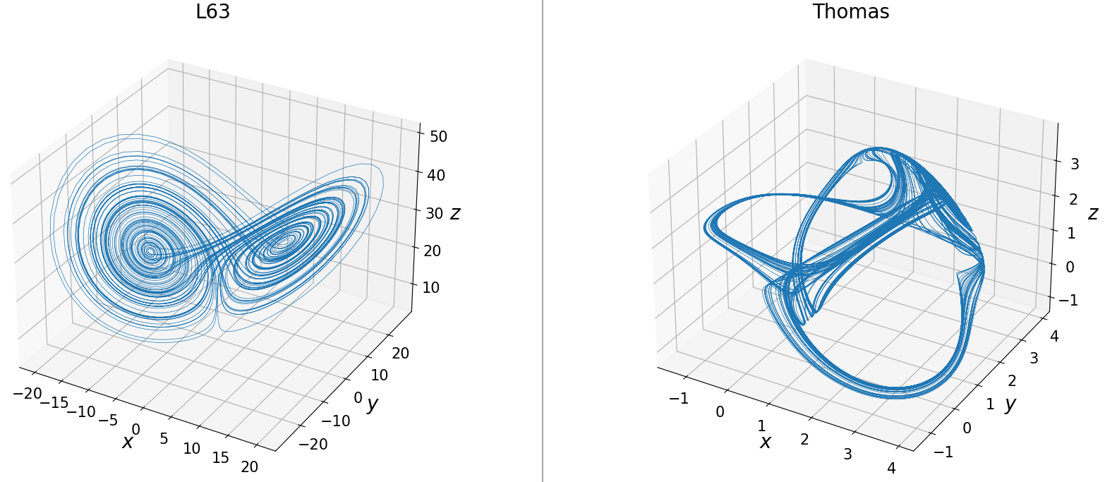
Figure 1: Attractors for non-gradient examples

4 Previous works

An extensive amount of work has been done on the topic of numerically solving Fokker-Planck equations. A large amount of these works are based on traditional PDE solving techniques like finite difference [4], [61], [53] and finite element [40], [39] methods. For a comparison of these traditional methods the reader can look at this comparative study [45] by Pitcher et al where the methods have been applied to 2 and 3 dimensional examples.

In recent times efforts have been made to devise methods that are applicable in dimensions higher than 3. Tensor decomposition methods [17], [28] are an important toolkit while dealing with high-dimensional problems and they are proving to be useful in designing numerical solvers for PDEs [2], [31]. For stationary Fokker-Planck equations Sun and Kumar proposed a tensor decomposition and Chebyshev spectral differentiation based method [57] in 2014. In this method drift functions are approximated with a sum of functions that are separable in spatial variables, an well-established paradigm for solving PDEs. The differential operator for the stationary FPE is then discretized and finally a least sqaures problem is solved to find the final solution. The normalization is enforced via addition of a penalty term in the optimization problem. The high-dimensional integral for the normalization constraint in this method is replaced with products of one dimensional integrals and therefore becomes computable.

In 2017 Chen and Majda proposed another hybrid method [9] that utilizes both kernel and sample based density approximation to solve FPEs that originate from a specific type of SDE referred to as a conditional Gaussian model,

(18) $$d\mathbf{u_{I}}=[A_{0}(t,\mathbf{u_{I}})+A_{1}(t,\mathbf{u_{I}})\mathbf{u_{II}}]\,dt+\Sigma_{I}(t,\mathbf{u_{I}})\,dW_{I}(t)$$

$$d\mathbf{u_{II}}=[a_{0}(t,\mathbf{u_{I}})+a_{1}(t,\mathbf{u_{I}})\mathbf{u_{II}}]\,dt+\Sigma_{II}(t,\mathbf{u_{I}})\,dW_{II}(t)$$

This special structure of the SDE allows one to approximate $p(\mathbf{u_{II}}(t))$ as a Gaussian mixture with parameters that satisfy auxiliary SDEs. $p(\mathbf{u_{I}}(t))$ is approximated with a non-parametric kernel based method. Finally the joint distribution $p(\mathbf{u_{I}}(t),\mathbf{u_{II}}(t))$ is computed with a hybrid expression. Using this method Chen and Majda computed the solution to a 6 dimensional conceptual model for turbulence. Note that, among our examples only L63 falls under this special structure.

In recent years machine learning has also been applied to solve SFPEs. In 2019 Xu et al solved 2 and 3 dimensional stationary FPEs with deep learning [62]. Their method enforced normalization via a penalty term in the loss function that represented a Monte-Carlo estimate of the solution integrated over $\mathbb{R}^{d}$. Although simple and effective in lower dimensions, this normalization strategy loses effectiveness in higher dimensions. Zhai et al [64] have proposed a combination of deep learning and Monte-Carlo method to solve stationary FPEs. The normalization constraint here is replaced with a regularizing term in the loss function which tries to make sure the final solution is close to a pre-computed Monte-Carlo solution. This strategy is more effective than having to approximate high-dimensional integrals and the authors successfully apply their method on Chen and Majda’s 6 dimensional example.

5 Overview of deep learning

In this section we describe the general process of learning a solution to a partial differential equation. The strategy described here will be an integral part of the final algorithm. In what follows next, we see how to see solve a generic PDE independent of time on a bounded domain with a Dirichlet boundary condition in a physics-informed manner. The interested reader can see [49], [5], [55] for more discussions. In the next few subsections we keep simplifying our PDE problem until it finally becomes solvable on a computer.

5.1 From PDE to optimization problem

In the context of machine learning, learning refers to solving an optimization problem. So to solve our PDE with deep learning we first transform it into an optimization problem. Suppose our 2nd order PDE looks like,

(19) $$\mathcal{L}f(\mathbf{x})=0,\quad\mathbf{x}\in\Omega\,,$$

$$f(\mathbf{x})=g(\mathbf{x}),\quad\mathbf{x}\in\partial\Omega\,,$$

and just like before we are interested in finding a solution in $W^{1,2}_{\rm loc}(\Omega)\cap C^{2}(\Omega)$. Instead of trying to solve (19) a popular strategy is to try to solve the following problem (see for example [55]),

(20) $$\underset{f\in W^{1,2}_{\rm loc}(\Omega)\cap C^{2}(\Omega)}{\rm arg\,inf}\left[\int_{\Omega}(\mathcal{L}f)^{2}+\int_{\partial\Omega}(f-g)^{2}\right]$$

The choice of function space ensures one-to-one correspondence between the solutions of the PDE and the optimization problem.

5.2 From infinite-dimensional search space to finite-dimensional search space

To solve a problem on a machine with finite resources we need to finitize the infinite aspects of the problem. We then solve the finitized problem which preferably approximates the original problem well to get an approximate solution to the orginal problem. For (20) our search space $W^{1,2}_{\rm loc}(\Omega)\cap C^{2}(\Omega)$ is infinite dimensional which we need to replace with a finite dimensional search space. In order to finitize the dimension of the search space we appeal to universal approximation theorems that say neural networks of even the simplest architectures are dense in continuous functions, see for example theorem 3.2 in [24] or proposition 3.7 in [46]. Universal approximation theorems typically allow networks to have either arbitrary depth or arbitrary width in order to achieve density [46], [12]. But the sets of neural networks with arbitrary depth or width are still infinite dimensional and therefore are infeasible to work with. In practice, we fix an architecture $\mathcal{A}$ with a fixed number of layers and trainable parameters and work with the following set instead.

(21) $$S_{\mathcal{A}}\stackrel{{\scriptstyle\rm def}}{{=}}\{n^{\mathcal{A}}_{\theta}:\theta\in\mathbb{R}^{C}\}$$

Here $n^{\mathcal{A}}_{\theta}$ is a network with architecture $\mathcal{A}$ with trainable parameters $\theta$ and $C$ is the total number of trainable parameters or the size of $\theta$. Since $C$ is fixed, $S_{\mathcal{A}}$ has a one-to-one correspondence with $\mathbb{R}^{C}$ and therefore is finite-dimensional. Even though we lose the density argument while working with $\theta$ of fixed size, in recent times it has been shown that sets like $S_{\mathcal{A}}$ are not closed in $W^{1,2}(\Omega)$ and $n^{\mathcal{A}}_{\theta}$ can be used as a good function approximator, see [38] for a detailed discussion. In the following discussion we suppress the architecture and use $n^{\mathcal{A}}_{\theta}$ and $n_{\theta}$ interchangably for notational convenience. After restricting our search space to (21), (20) becomes,

(22) $$\underset{\theta\in\mathbb{R}^{C}}{\rm arg\,inf}\left[\int_{\Omega}(\mathcal{L}n_{\theta})^{2}+\int_{\partial\Omega}(n_{\theta}-g)^{2}\right]$$

5.3 From integrals to sums

The domain $\Omega$ in our examples will often be of such a dimension that will make computing the integrals in (22) extremely challenging. To deal with this we will replace the integrals in (22) with Monte-Carlo sums as follows,

(23) $$\underset{\theta\in\mathbb{R}^{C}}{\rm arg\,inf}\left[\frac{1}{N}\sum_{j=1}^{N}(\mathcal{L}n_{\theta}(\mathbf{x}_{j}))^{2}+\frac{1}{M}\sum_{j=1}^{M}(n_{\theta}(\mathbf{y}_{j})-g(\mathbf{y}_{j}))^{2}\right]$$

where $\{\mathbf{x}_{j}\}_{j=1}^{N}$, $\{\mathbf{y}_{j}\}_{j=1}^{M}$ are uniform samples from $\Omega$ and $\partial\Omega$ respectively.

5.4 Finding the optimal parameters

We simply perform gradient descent with respect to $\theta$ to find the optimal network for the problem (23). The Monte-Carlo sample sizes should be dictated by the hardware available to the practitioner. In our experiments $N=M=1000$. In higher dimensions these choices are not enough to capture the original integrals entirely in one go. In that case (23) can interpreted as trying to find a network that satisfies the original problem (19) at the specified points $\{\mathbf{x}_{j}\}_{j=1}^{N},\{\mathbf{y}_{j}\}_{j=1}^{M}$, which we can refer to as collocation points. But in our experiments we try to the learn the solution on the entire domain as thoroughly as possible and so we resample the domain every few training iterations. So even though we are limited in sample-size by our hardware, we can shift the burden on space or memory to time or number of training iterations and adequately sample the entire domain. This principle of space-time trade-off is ubiquitous in machine learning [7] and comes in many different flavours like mini-batch gradient descent, stochastic gradient descent etc. Even though in this paradigm we are not training our network with typical input-output pairs, our method can be thought of as a variant of the mini-batch gradient descent.

5.5 Why deep learning

Deep learning in this context refers to learning an approximate solution to (19) with the outlined method with an architecture $\mathcal{A}$ that is deep or has many hidden layers. Deep networks are more efficient as approximators than shallow networks in the sense that they require far fewer number of trainable parameters to achieve the same level of approximation, for a discussion see section 5 of [20] or section 4 of [37]. Now that we have described the general procedure of deep learning a solution to a PDE, we will pause briefly to point out some benefits and demerits of this approach. Deep learning has, like any other method some disadvantages.

• Deep learning is slower and less accurate for lower dimensional problems for which standard solvers exist and have been in consistent development for many decades.

• Most modern GPUs are optimized for computation with single-precision or float32 numbers. This is efficient for rendering polygons or other image processing tasks which are the primary reasons GPUs were invented [44] but float32 might be not accurate enough for scientific computing. Although not ideal, this problem will most likely disappear in the future.

• The objective or loss function used in a typical problem might not be convex and hence difficult to deal with [32], [3].

But even with these disadvantages, the benefits of deep learning make it a worthwhile tool for solving PDEs.

• Since we don’t need to deal with meshes or grids in this method, we can mitigate the curse of dimensionality in memory. It will be clear from our experiments that the size of the network or $C$ does not need to grow exponentially with the dimensions. This method lets one compute the solution at collocation points but if one wants to compute the solution over the entire domain, one needs to sample the entire domain thoroughly which can be done in a sequential manner without requiring more memory as discussed in 5.4.

• All derivatives are computed with automatic differentiation and therefore are accurate upto floating point errors. Moreover, finite difference schemes do not satisfy some fundamental properties of differentiation e.g. the product rule [50]. With automatic differentiation one does not have to deal with such problems.

• If one computes the solution over the entire domain, the solution is obtained in a functional form which can be differentiated, integrated etc.

• Other than a method for sampling no modifications are required for accommodating different domains.

6 The algorithm

In this section we outline the algorithm for learning zeros of FPOs. But before that we go through the primary challenges and ways to mitigate them.

6.1 Unboundedness of the problem domain

We can try the same procedure as outlined in section 5 to solve find a non-trivial zero of $\mathcal{L}$. But since computationally we can only deal with a bounded domain, we focus on a compact domain which contains most of the mass of the solution to (1). We refer to this domain as the domain of interest $\Omega_{I}$ in the following discussion.

6.2 Existence of the trivial solution

$\mathcal{L}$, being a linear operator, $\mathcal{L}0=0$. Since we want to find a non-trivial zero of $\mathcal{L}$, we would like avoid the learning the zero function during the training of the network. To deal with this problem [64] added a regularization term that required solving (1) with Monte-Carlo first. Here we propose a method that does not require a priori knowing an approximate solution. Consider the operator $\mathcal{L}_{\rm log}$ instead.

(24) $$\mathcal{L}_{\rm log}f\stackrel{{\scriptstyle\rm def}}{{=}}e^{-f}\mathcal{L}e^{f}$$

Recalling (6) we see that,

(25) $$\mathcal{L}_{\rm log}f=-\nabla\cdot\mu-\mu\cdot\nabla f+D\left(\|\nabla f\|_{2}^{2}+\Delta f\right)$$

Since $\nabla\cdot\mu\not\equiv 0$, any constant function can not be a zero of $\mathcal{L}_{\rm log}$. $p$ is a zero of $\mathcal{L}$ iff either $p\equiv 0$ or $\log p$ is a zero of $\mathcal{L}_{\rm log}$. So we can look for a zero of $\mathcal{L}_{\rm log}$ to find a non-trivial zero of $\mathcal{L}$.

6.3 The steady state algorithm

The procedure outlined in section 5 together with the modifications in sections 6.1, 6.2 immediately yields the following loss function.

(26) $$L_{\log}=\frac{1}{N}\sum_{i=1}^{N}\mathcal{L}_{\rm log}(n_{\theta}(\mathbf{x}_{i}))^{2}$$

where $\{\mathbf{x}_{i}\}_{i=1}^{N}$ is a uniform sample from $\Omega_{I}$. Accordingly, the final procedure for finding a non-trivial zero of $\mathcal{L}$ is given in algorithm 1.

Sample $\{\mathbf{x}_{i}\}_{i=1}^{N}$ from $\Omega_{I}$, the domain of interest.

Select the desired architecture for $n_{\theta}$.

Select resampling interval $\tau$.

Select an adaptive learning rate $\delta$ and the number of training iterations $E$.

for $k=1,2\cdots,E$ do

       Compute $\nabla_{\theta}L_{\log}=\frac{1}{N}\sum_{i=1}^{N}\nabla_{\theta}(\mathcal{L}_{\log}(n_{\theta}(\mathbf{x}_{i}))^{2})$

       where $\mathcal{L}_{\log}f=-\nabla\cdot\mu-\mu\cdot\nabla f+D\left(\|\nabla f\|_{2}^{2}+\Delta f\right)$

       Update $\theta\leftarrow\theta-\delta\nabla_{\theta}L_{\log}$

       if $k\text{ is divisible by }\tau$ then

            Resample $\{\mathbf{x}_{i}\}_{i=1}^{N}$ from $\Omega_{I}$

       end if

      

end for

$e^{n_{\theta}(\mathbf{x})}$ is a non-trivial zero of $\mathcal{L}$.

Optional: Approximate $Z\leftarrow\int_{\mathbb{R}^{d}}e^{n_{\theta}(\mathbf{x})}\,d\mathbf{x}$. $\frac{1}{Z}e^{n_{\theta}(\mathbf{x})}$ is the learned, normalized steady state.

Algorithm 1 The steady state algorithm

In the following sections we describe in detail the network architecture and optimizer used in our experiments. Since the final solution is represented as $e^{n_{\theta}(\mathbf{x})}$, we have automatically secured positivity of the solution.

6.4 Architecture

We choose the widely used LSTM [54], [60] architecture described below for our experiments. This type of architecture rose to prominence in deep learning because of their ability to deal with the vanishing gradient problem, see section IV of [54], section 2.2 of [60]. A variant of this architecture has also been used to solve PDEs [55]. This kind of architectures have been shown to be universal approximators [52]. We choose this architecture simply because of how expressive they are. By expressivity of an architecture we imply its ability to approximate a wide range of functions and experts have attempted to formalize this notion in different ways in recent times [37], [47], [48]. There are architectures that are probability densities by design i.e. the normalization constraint in (1) is automatically satisfied for them, see for example [59], [43]. But our experiments suggest these architectures are not expressive enough to learn solutions to PDEs efficiently since the normalization constraint makes their structure too rigid. Other than the difficulty in implementing the normalization constraint numerically, this is another reason why we choose to focus on learning a non-trivial zero of $\mathcal{L}$ rather than solving (1). LSTM networks on the other hand are expressive enough to solve all the problems listed in section 3.

Below we define the our architecture in detail. Here $\mathbf{0}_{k}$ implies a zero vector of dimension $k$ and $\odot$ implies the Hadamard product.

(27) $$i\in\{1,2, \cdots,L\}$$

(28) $$\mathtt{c}_{0}(\mathbf{x})\stackrel{{\scriptstyle\rm def}}{{=}} \,\mathbf{0}_{m}$$

(29) $$\mathtt{h}_{0}(\mathbf{x})\stackrel{{\scriptstyle\rm def}}{{=}} \,\mathbf{0}_{d}$$

(30) $$\mathtt{f}_{i}(\mathbf{x})\stackrel{{\scriptstyle\rm def}}{{=}} \mathtt{A}(\mathtt{W}_{f}^{(i)}\mathbf{x}+\mathtt{U}_{f}^{(i)}h_{i-1}(\mathbf{x})+\mathtt{b}_{f}^{(i)})$$

(31) $$\mathtt{g}_{i}(\mathbf{x})\stackrel{{\scriptstyle\rm def}}{{=}} \mathtt{A}(\mathtt{W}_{g}^{(i)}\mathbf{x}+\mathtt{U}_{g}^{(i)}h_{i-1}(\mathbf{x})+\mathtt{b}_{g}^{(i)})$$

(32) $$\mathtt{r}_{i}(\mathbf{x})\stackrel{{\scriptstyle\rm def}}{{=}} \mathtt{A}(\mathtt{W}_{r}^{(i)}\mathbf{x}+\mathtt{U}_{r}^{(i)}h_{i-1}(\mathbf{x})+\mathtt{b}_{r}^{(i)})$$

(33) $$\mathtt{s}_{i}(\mathbf{x})\stackrel{{\scriptstyle\rm def}}{{=}} \mathtt{A}(\mathtt{W}_{s}^{(i)}\mathbf{x}+\mathtt{U}_{s}^{(i)}h_{i-1}(\mathbf{x})+\mathtt{b}_{s}^{(i)})$$

(34) $$\mathtt{c}_{i}(\mathbf{x})\stackrel{{\scriptstyle\rm def}}{{=}} \mathtt{f}_{i}(\mathbf{x})\odot\mathtt{c}_{i-1}(\mathbf{x})+\mathtt{g}_{i}(\mathbf{x})\odot s_{i}(\mathbf{x})$$

(35) $$\mathtt{h}_{i}(\mathbf{x})\stackrel{{\scriptstyle\rm def}}{{=}} \mathtt{r}_{i}(\mathbf{x})\odot\mathtt{A}(\mathtt{c}_{i}(\mathbf{x}))$$

(36) $$\mathtt{d}_{L}(\mathbf{x})\stackrel{{\scriptstyle\rm def}}{{=}} \mathtt{W}^{\top}\mathbf{x}+\mathtt{b}$$

(37) $$n^{\rm LSTM}_{\theta}\stackrel{{\scriptstyle\rm def}}{{=}} \mathtt{d}_{L}\circ\mathtt{h}_{L}$$

Here $\{\mathtt{f}_{i},\mathtt{g}_{i},\mathtt{r}_{i},\mathtt{s}_{i},\mathtt{c}_{i},\mathtt{h}_{i}:i=1,\cdots,L\}\cup\{\mathtt{d}_{L}\}$ are the hidden layers and

(38) $$\theta=\{\mathtt{W}_{f}^{(i)},\mathtt{U}_{f}^{(i)},\mathtt{b}_{f}^{(i)},\mathtt{W}_{g}^{(i)},\mathtt{U}_{g}^{(i)},\mathtt{b}_{g}^{(i)},\mathtt{W}_{r}^{(i)},\mathtt{U}_{r}^{(i)},\mathtt{b}_{r}^{(i)},\mathtt{W}_{s}^{(i)},\mathtt{U}_{s}^{(i)},\mathtt{b}_{s}^{(i)}:i=1,\cdots,L\}\cup\{\mathtt{W},\mathtt{b}\}$$

is the set of the trainable parameters. The dimensions of these parameters are given below,

(39) $$\mathtt{W}_{f}^{(i)},\mathtt{W}_{g}^{(i)},\mathtt{W}_{r}^{(i)},\mathtt{W}_{s}^{(i)}\in \;\mathbb{R}^{m\times d}$$

(40) $$\mathtt{U}_{f}^{(i)},\mathtt{U}_{g}^{(i)},\mathtt{U}_{r}^{(i)},\mathtt{U}_{s}^{(i)}\in \begin{cases}\mathbb{R}^{m\times d},\quad\text{ if }i=1\\ \mathbb{R}^{m\times m},\quad\text{otherwise}\end{cases}$$

(41) $$\mathtt{b}_{f}^{(i)},\mathtt{b}_{g}^{(i)},\mathtt{b}_{r}^{(i)},\mathtt{b}_{s}^{(i)}\in \;\mathbb{R}^{m}$$

(42) $$\mathtt{W}\in\mathbb{R}^{m},\mathtt{b}\in \;\mathbb{R}$$

which implies the size of the network or cardinality of $\theta$ is

(43) $$C=4m[d(L+1)+m(L-1)]+5m+1$$

Note that (43) implies the size of the network grows only linearly with dimension which is an important factor for mitigating the curse of dimensionality. We use elementwise $\tanh$ as our activation function,

(44) $$\mathtt{A}=\tanh$$

We use $m=50$ and $L=3$ for our experiments which implies our network has $6L+1=19$ hidden layers. We use the very popular Xavier or Glorot initialization [16], [11] to initialize $\theta$. With that, the description of our architecture is complete.

6.5 Optimization

In our experiments we use the ubiquitous Adam optimizer [26] which is often used in the PDE solving literature [18], [64], [55]. We use a piece-wise linear decaying learning rate. Below $k$ denotes the training iteration and $\delta(k)$ is the learning rate.

(45) $$\delta(k)=\begin{cases}5\times 10^{-3},\quad\text{if }k<1000\\ 1\times 10^{-3},\quad\text{if }1000\leq k<2000\\ 5\times 10^{-4},\quad\text{if }2000\leq k<10000\\ 1\times 10^{-4},\quad\text{if }k\geq 10000\\ \end{cases}$$

We stop training after reaching a certain number of iterations $E$ which varies depending on the problem. In all our experiments we use $N=1000$ as the sample size and $\tau=10$ as the resampling interval for algorithm 1.

7 Results

We are now ready to describe the results of our experiments. Next few sections parallel the examples in section 3 and contain problem-specific details about algorithm 1 e.g. $\Omega_{I},E$ etc. All computations were done with float32 numbers.

7.1 2D ring system

Figure 2 shows the learned and true solutions for the 2D ring system. Note that algorithm 1 produces an unnormalized zero of $\mathcal{L}$ but on the left panel the learned solution has been normalized for easier visualization.

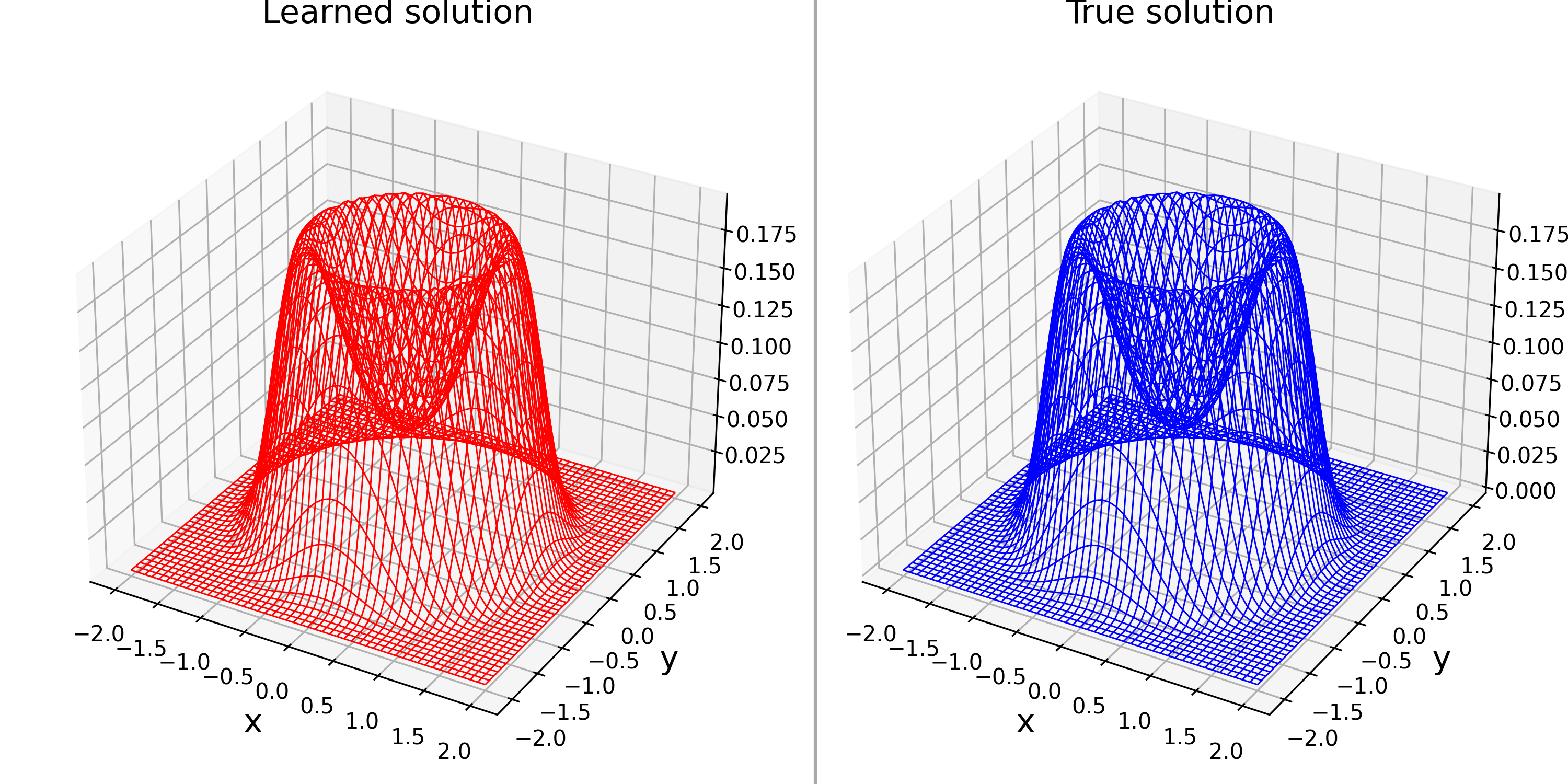
Figure 2: Solution for the 2D ring system

In this case we use $\Omega_{I}=[-2,2]^{2}$ and $E=8\times 10^{5}$ iterations.

7.1.1 Comparison with Monte Carlo

Since the network was trained with domain resampling every $10$ steps and a mini-batch size of $N=1000$, during the entire training procedure $8\times 10^{7}$ points were sampled from the domain. We compute the steady state with Monte Carlo with $8\times 10^{7}$ particles to compare errors produced by both methods. Here the SDE trajectories were generated till time 10 with time-steps of 0.01. Since in this case we know the analytic solution we can compute and compare absolute errors. As we can see in figure 3, for the same number of overall sampled points, Monte Carlo error is an order of magnitude larger than deep learning error.

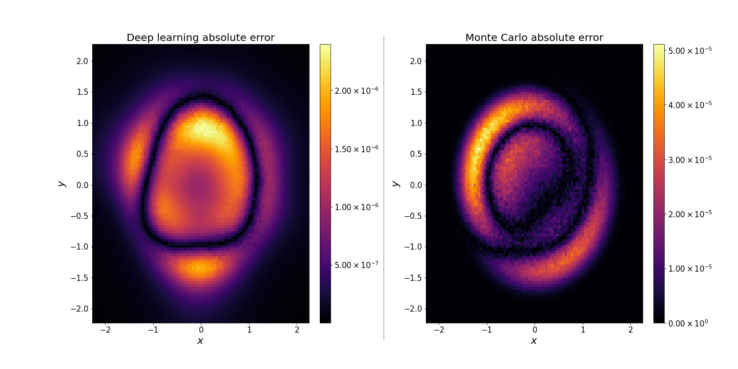
Figure 3: Comparison of absolute errors for deep learning and Monte Carlo solutions for the 2D ring system

7.2 2nD ring system

Although we solve this system for $n=1,2,3,4,5$, in this section we only produce the results for $n=5$ or $d=10$ to avoid repetition. Figure 4 shows the solutions for the 10D ring system for $\Omega_{I}=[-2,2]^{10}$ and $E=4.6\times 10^{6}$. In order to visualize the solution we focus on the quantity $p(0,0,0,0,x_{4},x_{5},0,0,0,0)$. For a visual comparison with the true solution normalization is desirable. But rather than trying to compute a 10-dimensional integral which is a non-trivial problem in itself we can normalize $p(0,0,0,0,x_{4},x_{5},0,0,0,0)$ which is much easier to do and due to the decoupled nature of this problem we can expect an identical result as in figure 2 which is what we see in figure 4. In both of the panels the solutions have been normalized in a way such that,

$$\int_{\mathbb{R}}\int_{\mathbb{R}}p(0,0,0,0,x_{4},x_{5},0,0,0,0)\,dx_{4}\,dx_{5}=1$$

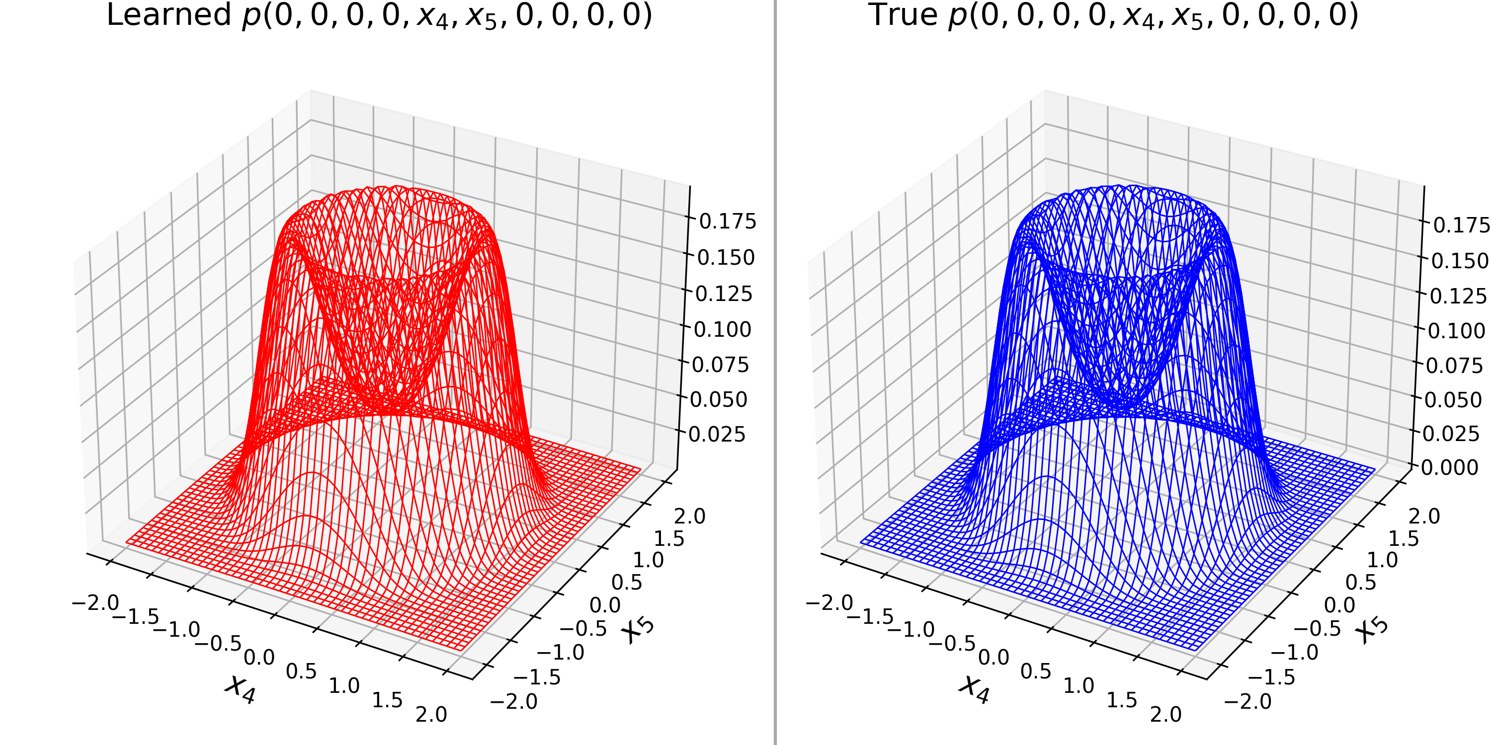
Figure 4: Solutions for the 10D ring system. Both solutions have been normalized such that $\int_{\mathbb{R}}\int_{\mathbb{R}}p(0,0,0,0,x_{4},x_{5},0,0,0,0)\,dx_{4}\,dx_{5}=1$

The error in the learned solution can be seen in figure 5.

Figure 5: Absolute error in the learned solution for the 10D ring system

7.3 Noisy Lorenz-63 system

Figure 6 shows the results for the L63 system for $\Omega_{I}=[-30,30]\times[-40,40]\times[0,70]$ and $E=10^{6}$. For ease of visualization the solutions have been normalized and in each row one of the dimensions has been integrated over the relevant interval to produce 2D marginals. In order to integrate out one dimension we use a composite Gauss-Legendre quadrature rule. We subdivide the relevant interval into 240 subintervals and use 10-point Gauss-Legendre rule to compute the integral over every subinterval. Note that since $n_{\theta}$ is a smooth function, our integrand is always a smooth function. The largest possible subinterval is of length $\frac{40-(-40)}{240}=\frac{1}{3}$ so assuming absolute value of the $20$-th derivative of the integrand is upper-bounded by $M$ everywhere, the integration error on each subinterval is upper-bounded by $\frac{2M}{20!}\left(\frac{1}{6}\right)^{20}\leq 2.25M\times 10^{-34}$, see appendix 9.3 for more details on this estimate. To produce the Monte Carlo solution, SDE trajectories were generated till time 10 with time-steps of $10^{-2}$. Since Monte Carlo produces lower-accuracy solutions even in lower dimensions as we saw in section 7.1.1 and an analytic solution is unavailable in this case, we refrain from producing error plots.

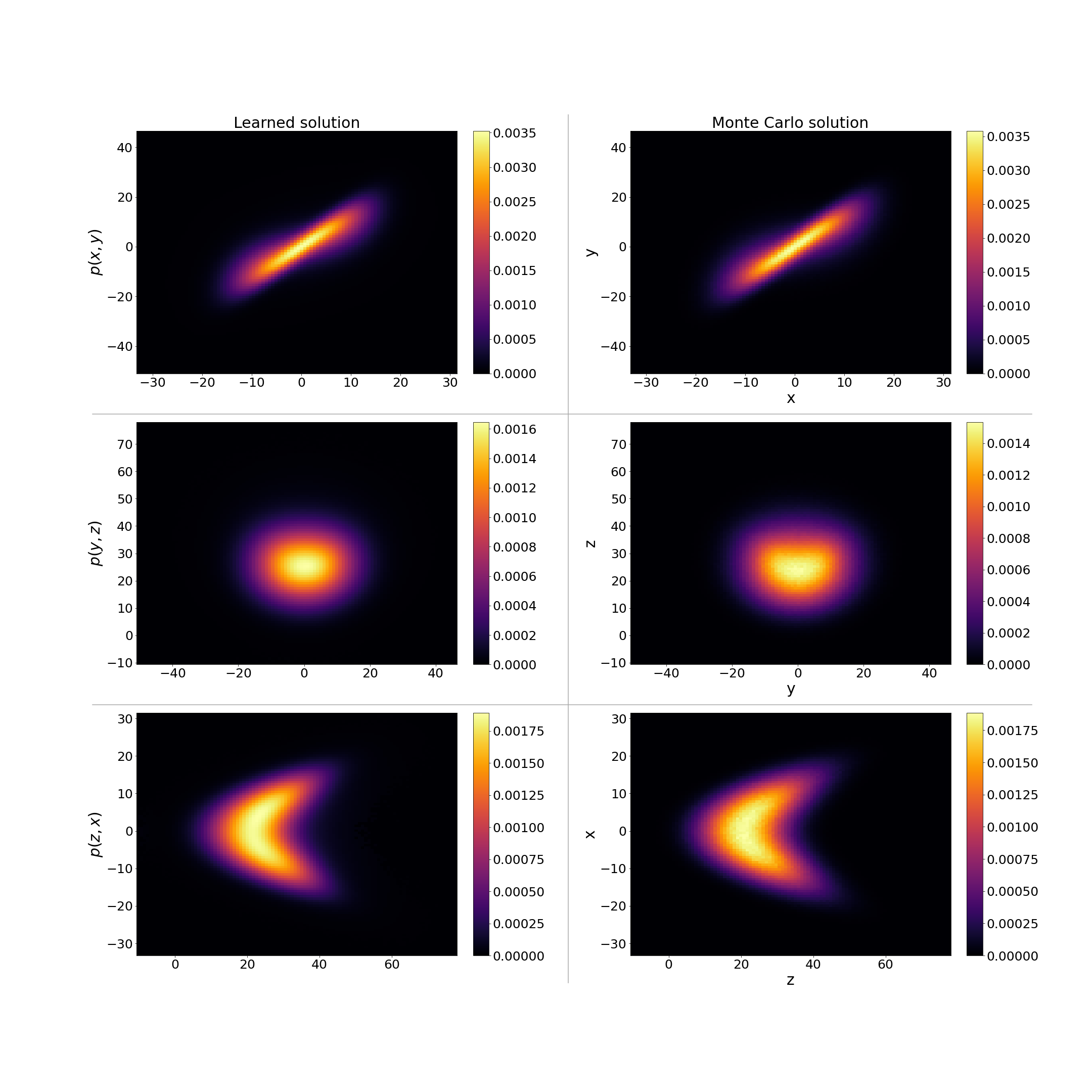
Figure 6: Solutions for the noisy Lorenz-63 system

7.4 Noisy Thomas system

Figure 7 shows the results for the Thomas system for $\Omega_{I}=[-10,10]^{3}$ and $E=4\times 10^{5}$. Due to the inherent symmetry of this problem it suffices to compute only the 2D marginal $p(x,y)$. To integrate out the $z$ dimension we use 8-point composite Gauss-Legendre quadrature rule with $165$ subintervals. Assuming absolute value of the $16$-th derivative of the integrand is upper-bounded by $M$ everywhere, the integration error on each subinterval is upper-bounded by $\frac{2M}{16!}\left(\frac{10}{165}\right)^{16}\leq 3.17M\times 10^{-33}$, see appendix 9.3 for more details on this error estimate. To produce the Monte Carlo solution, SDE trajectories were generated till time 10 with time-steps of $10^{-2}$. Even though we have solved a lower dimensional problem here, Thomas system turns out to be the easiest i.e. algorithm 1 converges faster for this system compared to the other ones as we will see in the next section.

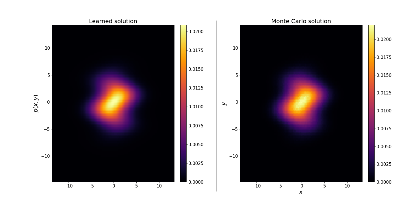
Figure 7: Solutions for the noisy Thomas system

7.5 Dimension dependence

In this section we explore the dimension dependence of algorithm 1. In the left panel of figure 8 we have plotted the loss given by (26) against training iterations for all the of the systems above in a semi-log manner starting from iteration $100$. We often encounter spikes in the loss curve for the following reasons

• the loss curves are single realizations of algorithm 1 instead of being an average

• we resample the domain every $10$ iterations and if the new points belong to a previously unexplored region in $\Omega_{I}$, the loss might increase.

But the general trend of loss diminishing with iterations is true for every system. We also see that loss is system-dependent and the hardness of these problems or how quickly algorithm 1 converges depends on the nature of $\mu$ as much as the dimension. This is easily seen by noting that the two 3D systems sandwich the 2D and the 4D ring systems in the left panel of figure 8. The loss for Thomas system drops very quickly compared to the rest of the systems due to the simplicity and global Lipschitzness of the corresponding drift function. We also see from the right panel of figure 8 that time taken per training iteration grows near-linearly with dimension. Since it is hard to estimate the amount of iterations to run before the loss drops below a pre-determined level, we refrain from plotting the total runtime of algorithm 1 against dimension. But it’s interesting to note that the number of total training iterations $E$ varies from $4\times 10^{5}$ to $4.6\times 10^{6}$ across all the problems. Since the data shown in the right panel of figure 8 is very much hardware dependent, at this point we disclose that all of the experiments were done using the cloud service provided by Google Colab. This service automatically assigns runtimes to different hardware depending on availability at the time of computation which might explain why the 8D and 10D ring systems take nearly the same amount of time per iteration in figure 8.

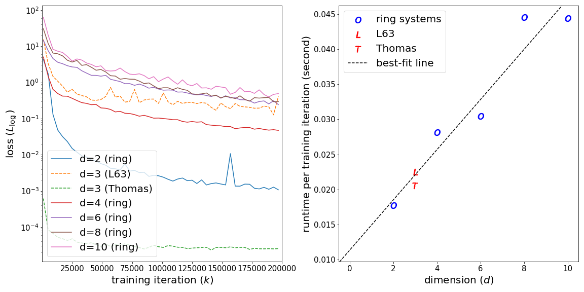
Figure 8: Left panel: Loss vs training iteration starting from iteration $100$. Right panel: time taken per training iteration vs dimension.

7.6 Comparison of loss and distance from truth

In this section we explore the relationship between the loss given by (26) and the distance from truth. In spite of being structurally completely different, both are measures of goodness for a computed solution. In most cases we only have access to the loss and therefore it is an important question if going a decreasing loss implies getting closer to the truth for algorithm 1. We define the distance of the learned zero from the true solution as follows,

(46) $$\|\phi\|_{*}\stackrel{{\scriptstyle\rm def}}{{=}}\sup_{\mathbf{x}\in\Omega_{I}}|c\phi(\mathbf{x})-p^{\rm true}(\mathbf{x})|,\qquad c\int_{\mathbb{R}^{d}}\phi=1$$

where $p^{\rm true}$ is the true solution to (1). (46) is not easy to compute in arbitrary dimensions but can be computed for the 2D ring system without too much effort since $p^{\rm true}$ is known and the problem is low-dimensional. Figure 9 shows the results for the 2D ring system. The right panel of figure 9 shows that loss and distance from truth are strongly correlated for algorithm 1. Moreover, asymptotically for small values of the loss function they are linearly related with a Pearson correlation coefficient $R=0.98$ as can be seen from the inset in the right panel which depicts the data from training iteration 10000 to 50000. The best-fit line is also shown in the inset. On the left panel we see that the distance from truth monotonically decreases with training iteration and is extremely well approximated by a curve of the form $a_{0}e^{-a_{1}k}+a_{2}$. Both panels contain data from training iteration 5000 to 50000. We omit the first few iterations to filter out the effects of the random initialization of the trainable parameters. Figure 9 serves as a good justification for algorithm 1 since it shows that minimizing the loss is akin to getting closer to a true non-trivial zero of $\mathcal{L}$.

Figure 9: Left panel: Distance from truth vs training iteration every 100 iterations, starting from iteration 5000 and ending at iteration 50000 for the 2D ring system. Right panel: Scatter plot for loss vs distance from truth for the 2D ring system. The inset shows that asymptotically loss and the distance from the truth are linearly related. The inset depicts the data from training iteration $10000$ to $50000$.

8 Conclusions

In this work we devise a deep learning algorithm for finding non-trivial zeros of $\mathcal{L}$ when the corresponding drift is non-solenoidal. We can summarize our results as follows.

1. Our choice of architecture is capable of learning zeros of Fokker-Planck operators across many different problems while scaling only linearly with dimension.

2. Time taken per training iteration grows near-linearly with problem dimension.

3. Apart from being able to produce solutions in a functional form which Monte Carlo is incapable of, for the same overall sample-size algorithm 1 produces more accurate solutions compared to Monte Carlo.

4. How quickly algorithm 1 converges to a zero depends as much on the dimension as it does on the nature of the problem or the structure of $\mu$.

5. By minimizing the loss we also get closer to a true non-trivial zero of the Fokker-Planck operator which justifies algorithm 1.

6. The loss and the distance from a true zero of the Fokker-Planck operator, even though structurally completely different, are strongly correlated. Moreover, they can be asymptotically linearly related for small values of the loss function.

In a sequel we will show how we can solve time-dependent FPEs by using the zeros learned by algorithm 1. The landscape of the loss defined in (1) poses many interesting geometric questions. For example, in case the nullspace of $\mathcal{L}$ is 1-dimensional do all the minima of $L_{\log}$ lie on a connected manifold of dimension $1$ or are they disconnected from each other? Such questions provide possible avenues for future research.

9 Appendix

9.1 Existence and uniqueness of solutions to example problems

In this section we prove that the example problems used here have a unique weak solution in $W^{1,2}_{\rm loc}(\mathbb{R}^{d})$. We employ the method of Lyapunov function as described in [21] to arrive at existence and uniqueness. First we begin with the prerequisites for this approach.

9.1.1 Lyapunov functions

Definition 9.1.

Let $U\in C(\mathcal{U})$ be a non-negative function and denote $\rho_{M}=\sup_{\mathbf{x}\in\mathcal{U}}U(\mathbf{x})$, called the essential upper bound of $U$. $U$ is said to be a compact function in $U$ if

(47) $$i)\;U(\mathbf{x})<\rho_{M},\quad\mathbf{x}\in U$$

and

(48) $$ii)\lim_{\mathbf{x}\to\partial U}U(\mathbf{x})=\rho_{M}$$

This definition of a compact function appears as definition 2.2 in [21].

Proposition 9.2.

An unbounded, non-negative function $U\in C(\mathbb{R}^{d})$ is compact iff

(49) $$\lim_{\|\mathbf{\mathbf{missing}}x\|_{2}\to+\infty}U(\mathbf{x})=+\infty$$

This proposition appears as proposition 2.1 in [21].

Definition 9.3.

Let $U$ be a compact function in $C^{2}(\mathcal{U})$ with essential upper bound $\rho_{M}$. $U$ is called a Lyapunov function in $\mathcal{U}$ with respect to $\mathcal{L}^{*}$ is $\exists\,\rho_{m}\in(0,\rho_{M})$ and a constant $\gamma>0$ such that

(50) $$\mathcal{L}^{*}U(\mathbf{x})\leq-\gamma,\qquad\forall\mathbf{x}\in\mathcal{U}\setminus\overline{\{\mathbf{x}\in\mathcal{U}:U(\mathbf{x})<\rho_{m}\}}$$

where $\mathcal{L}^{*}$ is the adjoint Fokker-Planck operator given by

(51) $$\mathcal{L}^{*}f=\mu\cdot\nabla f+D\odot\nabla^{2}f$$

This definition appears as definition 2.4 in [21]. Now we are ready to state the main theorem that will help us prove uniqueness for our example problems.

Theorem 9.4.

If the components of $\mu$ are in $L^{2}_{\rm loc}(\mathcal{U})$ and there exists a Lyapunov function with respect to $\mathcal{L}^{*}$ in $C^{2}(\mathcal{U})$ then (1) has a positive weak solution in the space $W^{1,2}_{\rm loc}(\mathcal{U})$. If, in addition, the Lyapunov function is unbounded, the solution is unique in $\mathcal{U}$.

This theorem appears as theorem $A$ in [21]. Since the components of $\mu$ are locally integrable for our example problems, all we need to do is find an unbounded Lyapunov function $U$ for proving existence and uniqueness in $W^{1,2}_{\rm loc}(\mathbb{R}^{d})$.

9.1.2 Existence and uniqueness of solution for 2D ring system

Setting

(52) $$\mathcal{U} =\mathbb{R}^{2}$$

(53) $$U(x,y) =x^{2}+y^{2}$$

(54) $$\rho_{m} =\frac{1}{2}+\sqrt{D+1}$$

(55) $$\gamma =4D+6$$

we see that,

(57) $$\mathcal{L}^{*}U+\gamma=-8\left(x^{2}+y^{2}-\frac{1}{2}\right)^{2}+8(D+1)$$

and,

(58) $$\mathcal{U}\setminus\overline{\{\mathbf{x}\in\mathcal{U}:U(\mathbf{x})<\rho_{m}\}}=\left\{(x,y)\in\mathbb{R}:x^{2}+y^{2}>\rho_{m}\right\}$$

In $\left\{(x,y)\in\mathbb{R}:x^{2}+y^{2}>\rho_{m}\right\}$,

(59) $$\mathcal{L}^{*}U+\gamma\leq 0$$

and therefore $U$ is an unbounded Lyapunov function for the 2D ring system which guarantees uniqueness of solution (11).

9.1.3 Existence and uniqueness of solution for L63 system

Setting,

(60) $$U(x,y,z)=\rho x^{2}+\alpha y^{2}+\alpha(z-2\rho)^{2}$$

we see that

(61) $$\mathcal{L}^{*}U =-2\alpha\rho x^{2}-2\alpha y^{2}-2\alpha\beta z^{2}+4\alpha\beta\rho z+2D(2\alpha+\rho)$$

(62) $$=-2\alpha\rho x^{2}-2\alpha y^{2}-\alpha\beta z^{2}-\alpha\beta(z-2\rho)^{2}+4\alpha\beta\rho^{2}+2D(2\alpha+\rho)$$

(63) $$\leq-\rho x^{2}-\alpha y^{2}-\alpha(z-2\rho)^{2}+4\alpha\beta\rho^{2}+2D(2\alpha+\rho)$$

(64) $$=-U(x,y,z)+4\alpha\beta\rho^{2}+2D(2\alpha+\rho)$$

(63) is a consequence of $\alpha,\beta,\rho>1$. Now setting,

(65) $$\gamma =1,$$

(66) $$\rho_{m} =4\alpha\beta\rho^{2}+2D(2\alpha+\rho)+1$$

we see that in $\{U>\rho_{m}\}$,

(67) $$\mathcal{L}^{*}U+\gamma\leq 0$$

So $U$ is an unbounded Lyapunov function for this system and we have a unique solution.

9.1.4 Existence and uniqueness of solution for Thomas system

Setting,

(68) $$U(x,y,z)=x^{2}+y^{2}+z^{2}$$

we see that

(69) $$\mathcal{L}^{*}U =x\sin y+y\sin z+z\sin x-b(x^{2}+y^{2}+z^{2})+6D$$

(70) $$\leq\sqrt{3U}-bU+6D$$

(71) $$=-b\left(\sqrt{U}-\frac{\sqrt{3}}{2b}\right)^{2}+\frac{3}{4b}+6D$$

(70) follows from Cauchy Schwarz inequality. Setting,

(72) $$\gamma =\frac{1}{4b},$$

(73) $$\rho_{m} =\left(\frac{\sqrt{3}}{2b}+\frac{\sqrt{1+6bD}}{b}\right)^{2}$$

we see that in $\{U>\rho_{m}\}$,

(74) $$\mathcal{L}^{*}U+\gamma\leq 0$$

So $U$ is an unbounded Lyapunov function for this system and we have a unique solution.

9.2 Monte Carlo steady state algorithm

The time-dependent FPE given by

(75) $$\frac{\partial p(t,\mathbf{x})}{\partial t}=\mathcal{L}p(t,\mathbf{x}),\qquad\mathbf{x}\in\mathbb{R}^{d},\;t\geq 0$$

$$p(0,\mathbf{x})=p_{0}(\mathbf{x}),\qquad\mathbf{x}\in\mathbb{R}^{d}$$

$$\int_{\mathbb{R}^{d}}p(t,\mathbf{x})\,d\mathbf{x}=1,\qquad\forall\;t\geq 0$$

gives us the probability density of the random process $X_{t}$ which is governed by the SDE,

(76) $$dX_{t}=\mu\,dt+\sigma\,dW_{t}$$

$$X_{0}\sim p_{0}$$

where $\{W_{t}\}$ is the standard Wiener process, see for example chapters 4, 5 of [15]. We can evolve $\eqref{algo:steady}$ up to sufficiently long time using Euler-Maruyama method [27] to approximate the steady state solution of (75) or the solution of (1) as follows. Here $\mathcal{N}$ denotes the multivariate normal distribution.

Sample $\{X_{0}^{(i)}\}_{i=1}^{N}\sim p_{0}$.

Set the time-step $h$.

Set the number of steps $S$.

for $k=1,2\cdots,S$ do

       Sample $w^{i}_{k}\sim\mathcal{N}(\mathbf{0}_{d},hI_{d})\;\;\forall\;i$

       $X_{k}^{(i)}\leftarrow X_{k-1}^{(i)}+\mu\left(X_{k-1}^{(i)}\right)h+\sigma w_{k}^{i}\;\;\forall\;i$

      

end for

Subdivide the domain of interest $\Omega_{I}$ into $d$-dimensional boxes.

Count the number of $X^{(i)}_{S}$ that are in a box to estimate the stationary density at the center of the box.

Algorithm 2 Monte Carlo steady state algorithm

Note that in case of a unique solution of (1), many choices of $p_{0}$ can lead to the stationary solution. In all our examples, it suffices to choose $p_{0}$ to be the standard $d$-dimensional normal distribution.

9.3 Integration error for $n$-point Gauss-Legendre rule

Suppose we are trying to integrate a smooth function $f(x)$ over $\left[a-\frac{h}{2},a+\frac{h}{2}\right]$ with $n$-point Gauss-Legendre rule where $h\in(0,1]$. Let us denote $I[f]$ to be the Gauss-Legendre approximation of $\int_{a-\frac{h}{2}}^{a+\frac{h}{2}}f(x)\,dx$. Recalling that $n$-point Gauss-Legendre gives us exact integrals for polynomial of degree $\leq 2n-1$ and using the Lagrange form of Taylor remainder we see that,

(77) $$\left|I[f]-\int_{a-\frac{h}{2}}^{a+\frac{h}{2}}f(x)\,dx\right| \leq MI\left[\frac{(x-a)^{2n}}{(2n)!}\right]+M\int_{a-\frac{h}{2}}^{a+\frac{h}{2}}\frac{(x-a)^{2n}}{(2n)!}\,dx$$

where $|f^{(2n)}(x)|\leq M\;\;\forall\;\;x\in\left[a-\frac{h}{2},a+\frac{h}{2}\right]$. To bound the first term on the RHS of (77) we can use the fact that if

(78) $$I[f]=\sum_{i=1}^{n}w_{i}f(x_{i})$$

then,

(79) $$I[1]=\int_{a-\frac{h}{2}}^{a+\frac{h}{2}}1\,dx=h$$

(80) $$\implies \sum_{i=1}^{n}w_{i}=h\leq 1$$

(81) $$\implies I\left[\frac{(x-a)^{2n}}{(2n)!}\right]\leq\frac{1}{(2n)!}\left(\frac{h}{2}\right)^{2n}$$

Therefore,

(82) $$\left|I[f]-\int_{a-\frac{h}{2}}^{a+\frac{h}{2}}f(x)\,dx\right|\leq\frac{M}{(2n)!}\left(\frac{h}{2}\right)^{2n}+\frac{2M}{(2n+1)!}\left(\frac{h}{2}\right)^{2n+1}\leq\frac{2M}{(2n)!}\left(\frac{h}{2}\right)^{2n}$$

References

- [1] L. J. Allen, An introduction to stochastic processes with applications to biology, CRC press, 2010.
- [2] J. Ballani and L. Grasedyck, A projection method to solve linear systems in tensor format, Numerical linear algebra with applications, 20 (2013), pp. 27–43.
- [3] S. Basir, Investigating and mitigating failure modes in physics-informed neural networks (pinns), arXiv preprint arXiv:2209.09988, (2022).
- [4] Y. A. Berezin, V. Khudick, and M. Pekker, Conservative finite-difference schemes for the fokker-planck equation not violating the law of an increasing entropy, Journal of Computational Physics, 69 (1987), pp. 163–174.
- [5] J. Blechschmidt and O. G. Ernst, Three ways to solve partial differential equations with neural networks—a review, GAMM-Mitteilungen, 44 (2021), p. e202100006.
- [6] H. Brezis and H. Brézis, Functional analysis, Sobolev spaces and partial differential equations, vol. 2, Springer, 2011.
- [7] N. Buduma, N. Buduma, and J. Papa, Fundamentals of deep learning, ” O’Reilly Media, Inc.”, 2022.
- [8] A. Carrassi, M. Bocquet, J. Demaeyer, C. Grudzien, P. Raanes, and S. Vannitsem, Data assimilation for chaotic dynamics, Data Assimilation for Atmospheric, Oceanic and Hydrologic Applications (Vol. IV), (2022), pp. 1–42.
- [9] N. Chen and A. J. Majda, Efficient statistically accurate algorithms for the fokker–planck equation in large dimensions, Journal of Computational Physics, 354 (2018), pp. 242–268.
- [10] P. A. Cioica-Licht, M. Hutzenthaler, and P. T. Werner, Deep neural networks overcome the curse of dimensionality in the numerical approximation of semilinear partial differential equations, arXiv preprint arXiv:2205.14398, (2022).
- [11] L. Datta, A survey on activation functions and their relation with xavier and he normal initialization, arXiv preprint arXiv:2004.06632, (2020).
- [12] T. De Ryck, S. Lanthaler, and S. Mishra, On the approximation of functions by tanh neural networks, Neural Networks, 143 (2021), pp. 732–750.
- [13] Ł. Delong, Backward stochastic differential equations with jumps and their actuarial and financial applications, Springer, 2013.
- [14] C. Gao, J. Isaacson, and C. Krause, i-flow: High-dimensional integration and sampling with normalizing flows, Machine Learning: Science and Technology, 1 (2020), p. 045023.
- [15] C. Gardiner, Stochastic methods, vol. 4, Springer Berlin, 2009.
- [16] X. Glorot and Y. Bengio, Understanding the difficulty of training deep feedforward neural networks, in Proceedings of the thirteenth international conference on artificial intelligence and statistics, JMLR Workshop and Conference Proceedings, 2010, pp. 249–256.
- [17] W. Hackbusch, B. N. Khoromskij, and E. E. Tyrtyshnikov, Hierarchical kronecker tensor-product approximations, in J. Num. Math., 2005.
- [18] J. Han, A. Jentzen, and W. E, Solving high-dimensional partial differential equations using deep learning, Proceedings of the National Academy of Sciences, 115 (2018), pp. 8505–8510.
- [19] A. Hinrichs, E. Novak, M. Ullrich, and H. Woźniakowski, The curse of dimensionality for numerical integration of smooth functions, Mathematics of Computation, 83 (2014), pp. 2853–2863.
- [20] J. Holstermann, On the expressive power of neural networks, 2023, https://arxiv.org/abs/2306.00145.
- [21] W. Huang, M. Ji, Z. Liu, and Y. Yi, Steady states of fokker–planck equations: I. existence, Journal of Dynamics and Differential Equations, 27 (2015), pp. 721–742.
- [22] M. Ivanov and V. Shvets, Method of stochastic differential equations for calculating the kinetics of a collision plasma, Zhurnal Vychislitelnoi Matematiki i Matematicheskoi Fiziki, 20 (1980), pp. 682–690.
- [23] N. E. KARoUI and M. Quenez, Non-linear pricing theory and backward stochastic differential equations, Financial mathematics, (1997), pp. 191–246.
- [24] P. Kidger and T. Lyons, Universal approximation with deep narrow networks, in Conference on learning theory, PMLR, 2020, pp. 2306–2327.
- [25] T. Kilpeläinen, Weighted sobolev spaces and capacity, Ann. Acad. Sci. Fenn. Ser. AI Math, 19 (1994), pp. 95–113.
- [26] D. P. Kingma and J. Ba, Adam: A method for stochastic optimization, arXiv preprint arXiv:1412.6980, (2014).
- [27] P. E. Kloeden, E. Platen, P. E. Kloeden, and E. Platen, Stochastic differential equations, Springer, 1992.
- [28] T. G. Kolda and B. W. Bader, Tensor decompositions and applications, SIAM review, 51 (2009), pp. 455–500.
- [29] V. Kontorovich and Z. Lovtchikova, Non linear filtering algorithms for chaotic signals: A comparative study, in 2009 2nd International Workshop on Nonlinear Dynamics and Synchronization, IEEE, 2009, pp. 221–227.
- [30] N. Kovachki, S. Lanthaler, and S. Mishra, On universal approximation and error bounds for fourier neural operators, The Journal of Machine Learning Research, 22 (2021), pp. 13237–13312.
- [31] D. Kressner and C. Tobler, Krylov subspace methods for linear systems with tensor product structure, SIAM journal on matrix analysis and applications, 31 (2010), pp. 1688–1714.
- [32] A. Krishnapriyan, A. Gholami, S. Zhe, R. Kirby, and M. W. Mahoney, Characterizing possible failure modes in physics-informed neural networks, Advances in Neural Information Processing Systems, 34 (2021), pp. 26548–26560.
- [33] T. Lelievre and G. Stoltz, Partial differential equations and stochastic methods in molecular dynamics, Acta Numerica, 25 (2016), pp. 681–880.
- [34] G. Leobacher and F. Pillichshammer, Introduction to quasi-Monte Carlo integration and applications, Springer, 2014.
- [35] E. N. Lorenz, Deterministic nonperiodic flow, Journal of atmospheric sciences, 20 (1963), pp. 130–141.
- [36] Y. Lu and J. Lu, A universal approximation theorem of deep neural networks for expressing probability distributions, Advances in neural information processing systems, 33 (2020), pp. 3094–3105.
- [37] Z. Lu, H. Pu, F. Wang, Z. Hu, and L. Wang, The expressive power of neural networks: A view from the width, Advances in neural information processing systems, 30 (2017).
- [38] S. Mahan, E. J. King, and A. Cloninger, Nonclosedness of sets of neural networks in sobolev spaces, Neural Networks, 137 (2021), pp. 85–96.
- [39] A. Masud and L. A. Bergman, Application of multi-scale finite element methods to the solution of the fokker–planck equation, Computer Methods in Applied Mechanics and Engineering, 194 (2005), pp. 1513–1526.
- [40] J. Náprstek and R. Král, Finite element method analysis of fokker–plank equation in stationary and evolutionary versions, Advances in Engineering Software, 72 (2014), pp. 28–38.
- [41] B. Øksendal and B. Øksendal, Stochastic differential equations, Springer, 2003.
- [42] E. Ott, Strange attractors and chaotic motions of dynamical systems, Reviews of Modern Physics, 53 (1981), p. 655.
- [43] G. Papamakarios, Neural density estimation and likelihood-free inference, arXiv preprint arXiv:1910.13233, (2019).
- [44] J. Peddie, The History of the GPU-New Developments, Springer Nature, 2023.
- [45] L. Pichler, A. Masud, and L. A. Bergman, Numerical solution of the fokker–planck equation by finite difference and finite element methods—a comparative study, in Computational Methods in Stochastic Dynamics, Springer, 2013, pp. 69–85.
- [46] A. Pinkus, Approximation theory of the mlp model in neural networks, Acta numerica, 8 (1999), pp. 143–195.
- [47] M. Raghu, B. Poole, J. Kleinberg, S. Ganguli, and J. Sohl-Dickstein, Survey of expressivity in deep neural networks, arXiv preprint arXiv:1611.08083, (2016).
- [48] M. Raghu, B. Poole, J. Kleinberg, S. Ganguli, and J. Sohl-Dickstein, On the expressive power of deep neural networks, in international conference on machine learning, PMLR, 2017, pp. 2847–2854.
- [49] M. Raissi, P. Perdikaris, and G. E. Karniadakis, Physics-informed neural networks: A deep learning framework for solving forward and inverse problems involving nonlinear partial differential equations, Journal of Computational physics, 378 (2019), pp. 686–707.
- [50] H. Ranocha, Mimetic properties of difference operators: product and chain rules as for functions of bounded variation and entropy stability of second derivatives, BIT Numerical Mathematics, 59 (2019), pp. 547–563.
- [51] H. Risken and H. Risken, Fokker-planck equation, Springer, 1996.
- [52] A. M. Schäfer and H. G. Zimmermann, Recurrent neural networks are universal approximators, in Artificial Neural Networks–ICANN 2006: 16th International Conference, Athens, Greece, September 10-14, 2006. Proceedings, Part I 16, Springer, 2006, pp. 632–640.
- [53] B. Sepehrian and M. K. Radpoor, Numerical solution of non-linear fokker–planck equation using finite differences method and the cubic spline functions, Applied mathematics and computation, 262 (2015), pp. 187–190.
- [54] A. Sherstinsky, Fundamentals of recurrent neural network (rnn) and long short-term memory (lstm) network, Physica D: Nonlinear Phenomena, 404 (2020), p. 132306.
- [55] J. Sirignano and K. Spiliopoulos, Dgm: A deep learning algorithm for solving partial differential equations, Journal of computational physics, 375 (2018), pp. 1339–1364.
- [56] R. Strauss and F. Effenberger, A hitch-hiker’s guide to stochastic differential equations, Space Science Reviews, 212 (2017), pp. 151–192.
- [57] Y. Sun and M. Kumar, Numerical solution of high dimensional stationary fokker–planck equations via tensor decomposition and chebyshev spectral differentiation, Computers & Mathematics with Applications, 67 (2014), pp. 1960–1977.
- [58] R. Thomas, Deterministic chaos seen in terms of feedback circuits: Analysis, synthesis,” labyrinth chaos”, International Journal of Bifurcation and Chaos, 9 (1999), pp. 1889–1905.
- [59] B. Uria, I. Murray, and H. Larochelle, Rnade: The real-valued neural autoregressive density-estimator, Advances in Neural Information Processing Systems, 26 (2013).
- [60] C. B. Vennerød, A. Kjærran, and E. S. Bugge, Long short-term memory rnn, arXiv preprint arXiv:2105.06756, (2021).
- [61] J. C. Whitney, Finite difference methods for the fokker-planck equation, Journal of Computational Physics, 6 (1970), pp. 483–509.
- [62] Y. Xu, H. Zhang, Y. Li, K. Zhou, Q. Liu, and J. Kurths, Solving fokker-planck equation using deep learning, Chaos: An Interdisciplinary Journal of Nonlinear Science, 30 (2020), p. 013133.
- [63] H. C. Yeong, R. T. Beeson, N. Namachchivaya, and N. Perkowski, Particle filters with nudging in multiscale chaotic systems: With application to the lorenz’96 atmospheric model, Journal of Nonlinear Science, 30 (2020), pp. 1519–1552.
- [64] J. Zhai, M. Dobson, and Y. Li, A deep learning method for solving fokker-planck equations, in Mathematical and Scientific Machine Learning, PMLR, 2022, pp. 568–597.