Multilevel leapfrogging initialization for quantum approximate optimization algorithm

Abstract

The quantum approximate optimization algorithm (QAOA) is a prospective hybrid quantum-classical algorithm widely used to solve combinatorial optimization problems. However, the external parameter optimization required in QAOA tends to consume extensive resources to find the optimal parameters of the parameterized quantum circuit, which may be the bottleneck of QAOA. To meet this challenge, we first propose multilevel leapfrogging learning (M-Leap) that can be extended to quantum reinforcement learning, quantum circuit design, and other domains. M-Leap incrementally increases the circuit depth during optimization and predicts the initial parameters at level $p+r$ ($r>1$) based on the optimized parameters at level $p$, cutting down the optimization rounds. Then, we propose a multilevel leapfrogging-interpolation strategy (MLI) for initializing optimizations by combining M-Leap with the interpolation technique. We benchmark its performance on the Maxcut problem. Compared with the Interpolation-based strategy (INTERP), MLI cuts down at least half the number of rounds of optimization for the classical outer learning loop. Remarkably, the simulation results demonstrate that the running time of MLI is 1/3 of INTERP when MLI gets quasi-optimal solutions. In addition, we present the greedy-MLI strategy by introducing multi-start, which is an extension of MLI. The simulation results show that greedy-MLI can get a higher average performance than the remaining two methods. With their efficiency to find the quasi-optima in a fraction of costs, our methods may shed light in other quantum algorithms.

I Introduction

With advancements in quantum computing technology, many quantum algorithms grover ; shor ; hhl ; qpca ; wan_1 ; wan_2 ; pan_1 ; pan_2 ; Yu1 ; Yu2 ; Yu3 ; Yu4 have demonstrated significant speed advantages in solving certain problems, such as unstructured database searching grover and solving equations hhl . However, noise and qubit limitations prevent serious implementations of the aforementioned quantum algorithms in the current noisy intermediate-scale quantum (NISQ) devices NISQ ; VQA_review2 . As such, hybrid quantum-classical algorithms adaptive-vqe ; adaptive-vqe1 ; QAS ; qubit-adaptive-vqe ; Huang ; qsvd ; VQSE ; Xuxiaosi ; autoencoder_enhance ; vqsd ; nonlinear ; poisson ; VQNHE ; Wu_2023 ; vqe are proposed to fully exploit the power of NISQ devices.

Quantum approximate optimization algorithm (QAOA) automatic ; minimum_vertex_cover ; alternating_QAOA_ansatz ; adaptive-qaoa ; phase_transition ; performance_QAOA ; benchmarking is a hybrid quantum-classical algorithm, presented by Farhi et al.qaoa to tackle combinatorial optimization problems such as $k$-vertex cover minimum_vertex_cover and exact cover exact_cover . In QAOA, the solution of the combinatorial optimization problem tends to be encoded as the ground state of the target Hamiltonian $H_{C}$. The ground state can be approximately obtained by the following steps VQA_review1 . (i) Build a parameterized quantum circuit by utilizing $p$-level QAOA ansatz TQA , where each level consists of two unitaries: one is generated by $H_{C}$, the other is generated by the initial Hamiltonian $H_{B}$ qaoa , and each level has two variational parameters $\gamma_{i}$ and $\beta_{i}$ with $i=1,...,p$, where $p$ is the circuit depth. (ii) Initialize $2p$ QAOA parameters for the quantum circuit. (iii) The quantum computer computes the expectation value of the output state and delivers the relevant information to the classical computer. (iv) The classical computer updates the parameters by the classical optimizer and delivers new parameters to the quantum computer. (v) Repeat (iii)-(iv) to maximize (or minimize) the expectation values until meeting a termination condition, and the quantum circuit outputs an estimate of the solution to the problem.

To find the quasi-optimal solutions (i.e., nearly global optima) of QAOA, the outer loop optimization tends to consume abundant costs to search for the quasi-optimal parameters of the parameterized quantum circuit tree-QAOA , which may become a performance bottleneck of QAOA TQA . Fortunately, the costs can be significantly reduced when QAOA starts with initial parameters that are in the vicinity of quasi-optimal solutions benchmarking_1 ; VQA_review1 ; bilinear . However, getting such high-quality initial parameters is intractable in a highly non-convex space INTERP where is inundated with low-quality local optima. Thus, searching for heuristic parameter initialization strategies to effectively tackle the problem becomes a pressing concern TQA . To visualize the properties of the space, we give figure 1 consisting of a tree-dimensional graph and a heat map graph to depict an energy landscape of the QAOA objective function for Maxcut. In this landscape, the redder region corresponds to higher-quality local optimal solutions.

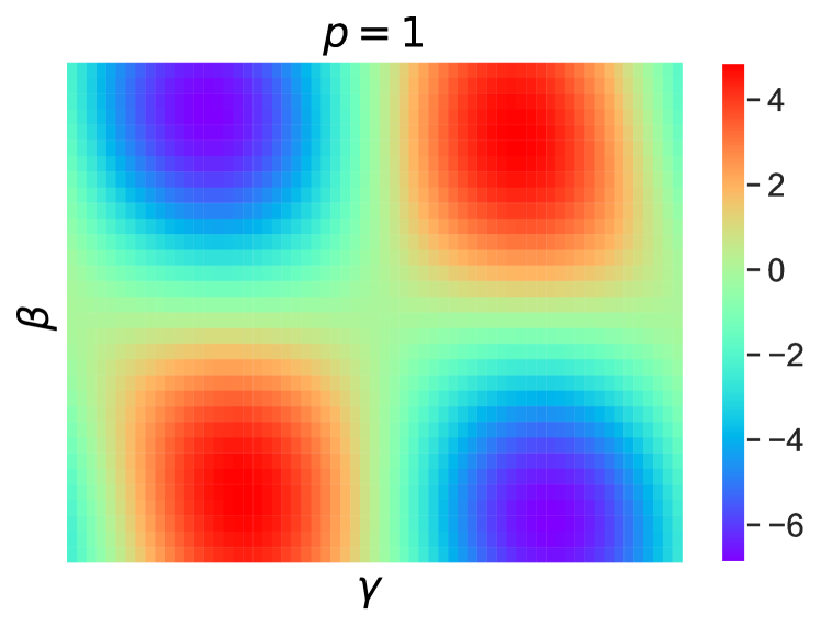
Figure 1: Energy landscape of QAOA objective function for Maxcut on a 3-regular graph with vertex number $n=10$. There are two variational parameters $\gamma$ and $\beta$ when $p=1$, where we restrict $\gamma\in\left[\frac{-\pi}{4},\frac{\pi}{4}\right)$ and $\beta\in\left[\frac{-\pi}{2},\frac{\pi}{2}\right)$ by symmetries as mentioned in reference  INTERP .

Recent studies of heuristic parameter initialization strategies mainly include two aspects. On the one hand, some studies predict QAOA parameters by taking advantage of machine learning techniques mc1 ; mc2 ; mc3 ; mc4 ; tree-QAOA . They offer the potential to efficiently find promising parameter values, which can help accelerate the convergence of QAOA and improve its performance on various optimization problems. However, the existing machine learning models have defects in generalization performance and numerous models are required for different problem sizes or QAOA depths PPN . On the other hand, there are some non-machine learning methods that initialize QAOA parameters based on the properties of the parameters leapfrogging ; INTERP ; multistart ; TQA ; fixing_strategy ; angle_conjecture ; bilinear , such as reusing the parameters from similar graphs leapfrogging and using the fixed angle conjecture angle_conjecture . Building on the observed pattern of the optimal parameters, Zhou et al. INTERP proposed an Interpolation-based strategy (INTERP), which performs linear interpolation on the optimized parameters at level $i-1$ to generate the initial guess parameters for level $i$, where $i=2,...,p$. INTERP can find the quasi-optimal solution in $O$[poly($p$)] optimization runs, while random initialization requires $2^{O(p)}$ optimization runs to achieve similar performance. Since the prediction of the new parameters at level $i$ depends on the optimized parameters at level $i-1$, INTERP requires executing one round of optimization at each level, consuming numerous costs to reach convergence for deep QAOA. Besides, there are other strategies layer_vqe ; bilinear ; recursive ; fixing_strategy facing the same problem, such as the bilinear strategy bilinear .

To meet this challenge, we first present multilevel leapfrogging learning (M-Leap) for parameterized quantum circuits. M-Leap is a training strategy where the circuit depth is incrementally grown during the optimization, and the initial parameters at level $i+r$ ($r>1$) are generated by the optimized parameters at level $i$, cutting down the optimization rounds. Then, we propose a multilevel leapfrogging interpolation strategy (MLI) by combining M-Leap with the interpolation technique, and we benchmark the performance of MLI on the Maxcut problem. MLI is an efficient heuristic approach for initializing optimizations. Compared with INTERP, MLI cuts down on at least half the number of rounds of optimization for the classical outer learning loop. The simulation results demonstrate that the running time of MLI is 1/3 of INTERP when MLI finds the quasi-optimal solution. In addition, we present greedy-MLI by introducing multi-start multistart , which is an extension of MLI. Greedy-MLI leverages parallel optimization to efficiently explore the parameter space, and it selectively preserves promising parameters, timely terminating the exploration of non-promising regions of the parameter space. These characteristics make greedy-MLI attain the quasi-optimal solution with less running time. Meanwhile, the simulation results show that greedy-MLI can get a higher average performance. With their ability to significantly reduce optimization rounds and achieve quasi-optimal solutions in a fraction of the time compared to existing approaches, our methods pave the way for more efficient quantum computation and optimization.

Though this paper specifically considers QAOA, the applications of M-Leap can be extended to various quantum computing tasks, such as quantum circuit design adaptive-vqe ; adaptive-vqe1 ; qubit-adaptive-vqe ; adaptive-qaoa ; QAS , quantum circuit learning QCL ; QCL2 and quantum machine learning mc1 ; mc2 ; mc3 , resulting in faster and more resource-efficient quantum computations across different application domains. In addition, MLI and greedy-MLI can be used as subroutines or preprocessing tools in other quantum optimization algorithms, accelerating the exploration of solution spaces and increasing the likelihood of finding near-global optima and better solutions to complex problems, thus enhancing the practicality of quantum optimization techniques.

The paper is organized as follows. Section II briefly reviews the Maxcut problem, QAOA, and INTERP. In section III, we first describe the idea of M-Leap, then propose two heuristic strategies for initializing optimization, that is, MLI and greedy-MLI. Subsequently, we compare the performance of three strategies in section IV. Finally, a short conclusion and discussion are given in section V.

II Preliminaries

II.1 Review of Maxcut

Maxcut is defined in graph $G=(V,E)$, where $V=\left\{{0,...,n-1}\right\}$ is the set of vertices, $E=\left\{(\left(u,v\right),w_{u,v})\right\}$ is the set of edges, $w_{u,v}$ is the weight of edge $(u,v)$ and $w_{u,v}=1$ in this paper. Maxcut aims at maximizing the number of cut edges by dividing $V$ into vertex subsets $S$ and $T$ that do not intersect each other maxcut ; perform1 .

In general, $x_{u}=1$ if the vertex $u$ is in the subset $S$, otherwise, $x_{u}=0$, where $u=0,1,...,n-1$. It is straightforward that every way of vertex partition corresponds to a unique bit string $x$, and there are $2^{n}$ forms for $x$ in total. The number of cut edges pluses one if vertices $u$ and $v$ of edge $e\in E$ are in distinct subsets of vertex, and the goal for Maxcut is to maximize the cost function

$$C(x)=\sum_{(u,v)\in E}x_{u}+x_{v}-2x_{u}x_{v}.$$ (1)

II.2 Review of QAOA

QAOA is a heuristic strategy motivated by adiabatic quantum computation adiabatic . The basic idea behind QAOA is to start from the ground state of the initial Hamiltonian $H_{B}$ and gradually evolve to the ground state of the target Hamiltonian $H_{C}$ through $p$-level QAOA ansatz qaoa . The initial Hamiltonian is conventionally chosen as $H_{B}=-\sum_{j=1}^{n}\sigma_{j}^{x}$ whose ground state $|s\rangle=|+\rangle^{\otimes n}$ can be effective to prepare. To encode the solution of Maxcut into the ground state of $H_{C}$, we convert the cost function $-C(x)$ to the target Hamiltonian

$$H_{C}=\sum_{(u,v)\in E}\frac{\sigma_{u}^{z}\sigma_{v}^{z}-I}{2}$$ (2)

by transforming each binary variable $x_{u}$ to a quantum spin $\frac{I-\sigma_{u}^{z}}{2}$, where $\sigma_{u}^{z}$ refers that applying Pauli-Z to the $u$-th qubit.

The ground state of $H_{C}$ can be approximately prepared by alternately applying unitaries $e^{-i\gamma_{i}H_{C}}$ and $e^{-i\beta_{i}H_{B}}$ on the initial quantum state $|s\rangle$. The prepared quantum state is

$$|\bm{\gamma_{p}},\bm{\beta_{p}}\rangle=e^{-i\beta_{p}H_{B}}e^{-i\gamma_{p}H_{C}}...e^{-i\beta_{1}H_{B}}e^{-i\gamma_{1}H_{C}}|s\rangle,$$ (3)

where $\bm{\gamma_{p}}=(\gamma_{1},...,\gamma_{p})$ and $\bm{\beta_{p}}=(\beta_{1},...,\beta_{p})$ are $2p$ variational QAOA parameters. We then define the expectation value $F(\bm{\gamma_{p}},\bm{\beta_{p}})$ of $H_{C}$ in this variational quantum state, where

$$F({\bm{\gamma_{p}}},{\bm{\beta_{p}}})=-\langle{\bm{\gamma_{p}}},{\bm{\beta_{p}}}|H_{C}|{\bm{\gamma_{p}}},{\bm{\beta_{p}}}\rangle,$$ (4)

which is done by repeated measurements of the quantum system using the computational basis and our goal is to search for the global optimal parameters

$$(\bm{\gamma_{p}}^{opt},\bm{\beta_{p}}^{opt})=\arg\underset{(\bm{\gamma_{p}},\bm{\beta_{p}})}{\max}F(\bm{\gamma_{p}},\bm{\beta_{p}}).$$ (5)

This search is typically done by starting with some initial guess of the parameters and performing optimization INTERP . To quantify the quality of QAOA solution, we introduce the approximation ratio

$$r=\frac{F({\bm{\gamma_{p}}},{\bm{\beta_{p}}})}{C_{max}},$$ (6)

where $C_{max}$ is the maximum cut value for the graph. The approximation ratio reflects how close the solution given by QAOA is to the true solution, $0\leq r\leq 1$, with the value of 1 nearer to the true solution bilinear .

II.3 Review of INTERP

For the Maxcut problem on 3-regular graphs, Zhou et al. INTERP presented INTERP building on the observed patterns in optimal parameters, where the optimal $\gamma_{i}^{*}$ tends to increase smoothly with $i=1,2,...,p$, whereas $\beta_{i}^{*}$ tends to decrease smoothly, such as shown in figure 2. The smooth pattern means that the variational QAOA parameters change gradually and continuously as the QAOA depth increases, without sharp jumps or discontinuities recursive . The smoothness property can be visually inspected by plotting the changes of QAOA angles as a function of $p$ and observing whether the curve appears continuous and smooth.

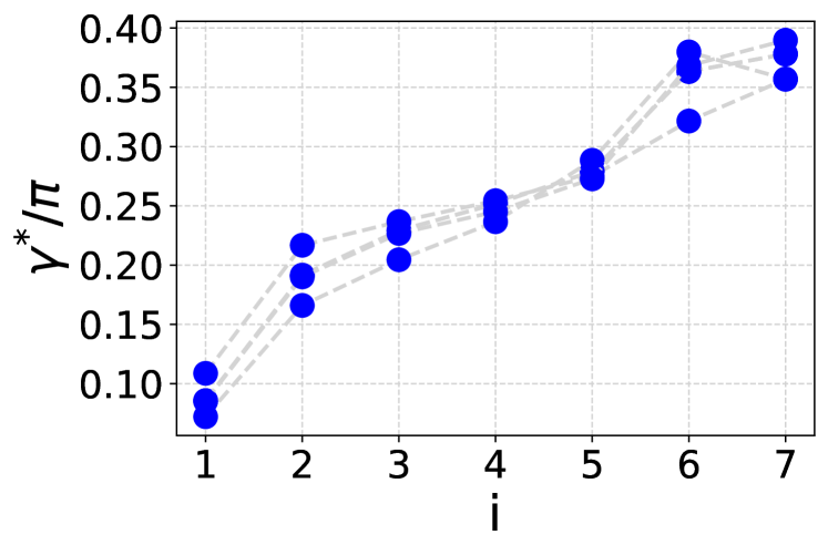
Figure 2: Smooth QAOA parameters at level $p=7$ for 3-regular graphs with $n=8$. Here, X-axis means the $i$-th level. Y-axis represents the value of the $i$-th optimal QAOA parameter.

In the following, we provide a detailed description of INTERP, as well as the relevant routine as shown in algorithm 1. The strategy works as follows: INTERP optimizes QAOA parameters starting from level $i=1$ and increments $i$ by one after optimizing. For $i\geq 2$, INTERP produces the initial guess of parameters for level $i$ by applying linear interpolation to the optimized parameters at level $i-1$, then optimizes 2$i$ QAOA parameters and increments $i$ by one after optimization. INTERP repeats the above process until it gets the optimized parameters at the target level $p$. In addition, we give figure 3 to help readers understand the process of generating initial points by taking advantage of interpolation.

Algorithm 1 Interpolation-based strategy

1:The target level $p$, random initial parameters $(\bm{\gamma_{i}}^{0},\bm{\beta_{i}}^{0})$ at level $i=1$;

2:The optimized parameters $(\bm{\gamma_{p}}^{*},\bm{\beta_{p}}^{*})$ at level $p$;

3:Optimize initial parameters $(\bm{\gamma_{i}}^{0},\bm{\beta_{i}}^{0})$ to get optimized parameters $(\bm{\gamma_{i}}^{*},\bm{\beta_{i}}^{*})$;

4:Update $i=i+1$ and generate the initial guess parameters $(\bm{\gamma_{i}}^{0},\bm{\beta_{i}}^{0})$ for level $i$ with the help of the optimized parameters $(\bm{\gamma_{i-1}}^{*},\bm{\beta_{i-1}}^{*})$;

5:Repeat $1-2$ until getting optimized parameters of the target level $p$.

Figure 3: A graphic example of interpolation. From $p$ to $p+l$, it respectively corresponds to one round of interpolation and multi-interpolation when $l=1$ and $l>1$. In each round of interpolation, the first and last parameters are unaltered, but the initial guess of the $t$-th point at level $p+1$ is altered by the $(t-1)$-th and $t$-th parameters at level $p$, where $t=2,...,p-1$. In the example, we generate the initial guess points for level $p=6$ by applying four consecutive interpolation to the optimized parameters at level $p=2$, where the arrows represent the order of interpolation and the dots in the line corresponds to the initial guess parameters for level $p\geq 3$.

III Related work

Since the initial angles at level $i+1$ are based on the optimized parameters at level $i$, INTERP needs optimization at each level, which means that the strategy tends to expend more costs as the level increases. Besides, there are some heuristics approaches fixing_strategy ; recursive ; INTERP ; bilinear ; layer_vqe confronting the same problem, which motivates us to search for heuristic approaches to reduce the costs of the outer loop optimization. In this section, we first investigate multilevel leapfrogging learning for the parameterized quantum circuit and provide a detailed description. Then, we present two classes of heuristic strategies called MLI and greedy-MLI for producing initial QAOA parameters, which combine M-Leap and the interpolation technique. These approaches hold the promise of reducing the costs associated with outer loop optimization, making them valuable tools in optimizing quantum circuits and QAOA applications.

Figure 4: The performance of MLI versus the circuit depth and the depth step $l$. For each $l$, MLI achieves better performances as the circuit depth increases. (Left) The optimal performance of MLI at each circuit depth. The inset depicts the optimal performance of MLI versus the depth step when $p=10$, we note MLI can obtain the identically optimal performance as INTERP at the target level. (Right) The average performance of MLI versus the circuit depth, and the inset reflects the effects of $l$ on the performance of MLI. MLI obtains better average performance than INTERP when $l=5$.

Algorithm 2 MLI strategy

1:The target level $p$, the list $q$, random initial parameters $(\bm{\gamma_{i}}^{0},\bm{\beta_{i}}^{0})$ at level $i=q[j]$.

2:The optimized parameters $(\bm{\gamma_{p}}^{*},\bm{\beta_{p}}^{*})$ at level $p$.

3:Optimize initial parameters $(\bm{\gamma_{i}}^{0},\bm{\beta_{i}}^{0})$ to get optimized parameters $(\bm{\gamma_{i}}^{*},\bm{\beta_{i}}^{*})$.

4:Update the index $j=j+1$ and generate the initial guess parameters for level $q[j]$ by applying linear interpolation to the optimized parameters at level $q[j-1]$.

5:Repeat $1-2$ until getting optimized parameters of the target level.

III.1 M-Leap

M-Leap is a training strategy that the circuit depth is incrementally grown during optimization, and the initial parameters at level $q_{0}+l$ are determined by the optimized parameters at level $q_{0}$, where $1\leq q_{0}<p$ and $1\leq l\leq p-q_{0}$. The strategy aims to address some of the challenges associated with training large quantum circuits and consists of two phases as follows.

Phase $\bm{1}$: The first phase is to pre-train a shallow quantum circuit with $q_{0}$-level ansatz (e.g., $q_{0}=2$) by complete-depth learning (CDL) layer_vqe , a training strategy where the circuit depth grows level by level and all parameters are updated in each training step. We aim to use some pre-information provided by the pre-trained layer to train a larger circuit in the second phase.

Phase $\bm{2}$: The second phase is to train a larger circuit by multilevel leapfrogging. The detailed steps are as follows: (i) Add $l$-level ansatz to the trained layer to construct a circuit with $(q_{0}+l)$-level ansatz, where the value of $l$ is variable. (ii) Produce the initial guess of the parameters for level $q_{0}+l$ by the optimized parameters at level $q_{0}$, where we call this process multilevel leapfrogging initialization. There are some heuristic methods of initializing parameters. For example, we can generate the initial guess by consecutively applying the interpolation operation INTERP or bilinear operation bilinear into the optimized parameters at level $q_{0}$. In addition, we can also initialize the newly added parameters as zero layer_vqe , and the rest of the parameters can reuse the optimized parameters of the previous $q_{0}$-level fixing_strategy . (iii) Train all parameters or selectively train the parameters of certain levels, depending on the specific requirements. Update $q_{0}=q_{0}+l$. (iv) Repeat (i)-(iii) until getting $2p$ optimized parameters.

The optimization rounds of M-Leap are relevant to the value of the depth step $l$. For simplicity, we introduce a list $q$ to store the levels at which M-Leap performs optimization, where the elements of $q$ are incremental. For M-Leap, the list $q=[1,...,q_{0},p]$ when $l=p-q_{0}$ and $q=[1,2,...,p]$ when $l$ identically equals to one. The rounds in one optimization run decrease as $l$ increases. Thus, M-Leap reduces costs for the outer loop optimization. However, we have to admit that M-Leap may have low performance when $l$ is greater than a certain value. We think it is because there is not enough prior information to produce high-quality initial parameters when $l$ is large. In our following work, we investigate two heuristic strategies and explore how the value of $l$ affects our approaches.

III.2 MLI

MLI is a heuristic parameter initialization approach that combines M-Leap and the interpolation technique. The corresponding routine of MLI is in algorithm 2, where $j$ starts from 0.

In our preliminary work, we set $l=p-q_{0}$ (i.e., $q=[1,...,q_{0},p]$) and generate the initial guess of parameters for the target level $p$ by applying consecutive interpolations to the optimized parameters at level $q_{0}$, where we restrict $p>3$ and $2\leq q_{0}\leq p-2$. What calls for attention is that we pre-train the circuits with $q_{0}$-level by the steps in algorithm 1, which is slightly different from the first phase in M-Leap. INTERP is a special case of MLI, which is with $q_{0}=p-1$ (i.e., $l$ is the constant one). For the following simulations, we first randomly generate several 3-regular graphs with vertex number $n=10$ by the Python library networkx. Then, we explore the performance of MLI on given graphs when $l$ takes different values. We fix the target level $p=n$ and respectively perform 500 optimization runs of INTERP and MLI, where two strategies start from the same initial parameters. For ease of expression, the corresponding value of $l$ is represented as $l^{a}$ when MLI can get the quasi-optimal solution at the target level. The corresponding pre-trained layer of $l^{a}$ consists of $q_{0}^{a}$-level ansatz.

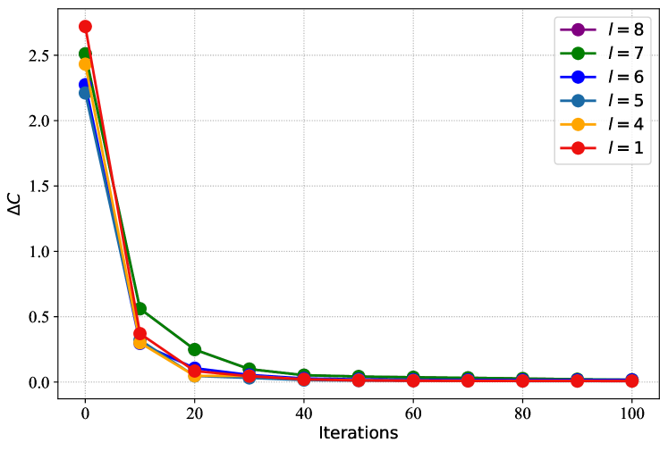
Figure 5: The changes of $\Delta C$ versus the number of iterations, where $\Delta C$ is the difference between current cost function value and $C_{max}$. The results reflect that the initial parameters produced by MLI can make the cost function rapidly converge.

Figure 6: The procedure of searching for the best value  $l^{*}$ (or $l^{a}$). The list $s$ stores the values of $l^{a}$, where $l^{*}$ is the largest value in the list $s$.

Figure 4 plots the approximation ratio obtained by MLI versus the circuit depth and the depth step $l$. Clearly, MLI obtains higher approximation as the circuit depth increases. MLI consistently attains the identical optimal approximation ratio with INTERP under different values of $l^{a}$ (e.g., $l^{a}=4,5,6$). Additionally, MLI improves the average performance compared to INTERP when $l^{a}=5$. In figure 5, we display the difference value $\Delta C$ versus the number of iterations (with the maximum number of iterations fixed). The cost function gradually converges towards the quasi-optimal value as the number of iterations increases. While we performed many runs, this plot shows only the run where MLI and INTERP achieved the lowest $\Delta C$ at the target level. The simulation results indicate that the convergence speed of the cost function remains relatively consistent even though QAOA starts from different initial parameters when $l=1,4,5,6$. It is essential to highlight that an arbitrary increase in $l$ may lead to a decline in the performance of MLI, resulting in slower convergence or potential entrapment in local optima, as evident in both figure 4 and figure 5. Overall, the findings suggest that MLI achieves performance on par with INTERP while operating at a lower expenditure.

In this paper, we represent the largest value of $l^{a}$ as $l^{*}$, which makes MLI get the quasi-optimal parameters consuming the least costs. We find $l^{*}$ by the following steps. (i) Assume the initial value of $l$ is $p-\left\lceil\frac{p}{2}\right\rceil$. (ii) Get the optimized parameters at level $q_{0}$, where $q_{0}=p-l$. (iii) Produce the initial guess parameters $(\bm{\gamma_{p}}^{0},\bm{\beta_{p}}{0})$ by applying successive linear interpolations to $(\bm{\gamma_{q_{0}}}{*},\bm{\beta_{q_{0}}}{*})$, then optimize $(\bm{\gamma_{p}}^{0},\bm{\beta_{p}}{0})$ to get the expectation value at the target level. (iv) Calculate the difference $\Delta F$ between $F(\bm{\gamma_{p}^{m}},\bm{\beta_{p}^{m}})$ and the quasi-optimal solution obtained by performing O[poly($p$)] optimization runs of INTERP, where $F(\bm{\gamma_{p}}^{m},\bm{\beta_{p}}{m})$ is the largest expectation value in multiple optimization runs of MLI. If $\Delta F=0$, that is, we get $l^{a}$, we append the value of $l$ into the list $s$, then increment $l$ by one. Otherwise, update $l=l-1$. (v) Repeat (ii)-(iv) until reaching the stop condition. The process of finding $q^{*}$ is shown in figure 6.

Table 1: The comparison of the optimal performance between INTERP and MLI with various $q$

Level	INTERP	MLI
		$q=[1,2,4,6,10]$	$q=[1,2,4,10]$	$q=[1,2,5,10]$	$q=[1,2,6,10]$
$p=1$	5.1566	5.1566	5.1566	5.1566	5.1566
$p=2$	7.9621	7.9621	7.9621	7.9621	7.9621
$p=3$	9.5645
$p=4$	10.1791	10.1791	10.1791
$p=5$	10.5699			10.5699
$p=6$	10.7899	10.7899			10.7899
$p=7$	10.9265
$p=8$	10.9618
$p=9$	10.9839
$p=10$	10.9927	10.9927	10.9927	10.9927	10.9927

Table 2: The comparison of average performance between INTERP and MLI with various $q$

Level	INTERP	MLI
		$q=[1,2,4,6,10]$	$q=[1,2,4,10]$	$q=[1,2,5,10]$	$q=[1,2,6,10]$
$p=1$	5.1566	5.1566	5.1566	5.1566	5.1566
$p=2$	7.9621	7.9621	7.9621	7.9621	7.9621
$p=3$	9.5645
$p=4$	10.1791	9.9937	9.9937
$p=5$	10.5699			10.3774
$p=6$	10.7917	10.428			10.6509
$p=7$	10.8463
$p=8$	10.8814
$p=9$	10.9
$p=10$	10.9460	10.9460	10.9578	10.9078	10.8449

For the above instance, MLI reduces $l^{a}-1$ rounds of optimization when it gets the quasi-optimal solution. However, getting the optimized parameters at level $q_{0}^{a}$ by INTERP still requires numerous costs when $q_{0}^{a}$ is large. To further cut down on costs during the optimization of MLI, we adopt a recursive step to simplify $q=[1,...,q_{0}^{a},p]$: (i) Reset the target level to $p=q_{0}^{a}$. (ii) Use the preliminary idea of MLI to train a circuit with $p$-level QAOA ansatz, and search for the new value of $q_{0}^{a}$. (iii) Repeat (i) and (ii) until $p\leq 3$. In our subsequent work, we simplify $q=[1,...,q_{0}^{a},p]$ by the above recursive idea and perform 500 optimization runs of MLI. The comparable results in table 1 suggest that MLI can get the quasi-optima by the simplified $q$, such as $q=[1,2,4,10]$. At this time, MLI saves about half the number of rounds of optimization compared with INTERP. Besides, the numerical results in table 2 demonstrate that the average performance of MLI is better than INTERP when $q=[1,2,4,10]$. We attribute the feasibility of MLI to the conjecture that the parameters that make the objective function value converge may cluster in a region param_concentration ; angle_conjecture ; INTERP . When the optimized parameters at level $q[j-1]$ tend to change smoothly, the initial parameters for level $q[j]$ obtained by multi-interpolation are near the region, and we may get high-quality local maxima after optimization.

The list $q^{*}$ cuts down the most costs under the condition that MLI can get the same quasi-optimal value as INTERP, and it consists of $q_{0}^{*}$ and the level $i=1,2,p$. We can get $q^{*}$ by the following recursive steps: (i) For the target level $p$, search for $l^{*}$, $q_{0}^{*}=p-l^{*}$. (ii) Reset the target level $p=q_{0}^{*}$. (iii) Explore the new value of $q_{0}^{*}$ by figure 6. (iv) Repeat (ii) and (iii) until the target level $p\leq 3$. In our work, we randomly generate 90 3-regular graphs with $n=6,8,10,12,14$ and seek the list $q^{*}$ based on them. From the numerical results, we find that $q_{0}^{*}$ approximates $\frac{p}{2}-1$ when the target level $p>4$ and $p$ is even, $q_{0}^{*}$ approaches $\frac{p-1}{2}$ when the target level $p>4$ and $p$ is odd, and $q_{0}^{*}$ equals 2 when $p=4$. Though numerous costs are required to search for the simplified $q$ that are ”universally good”, the obtained regularities can provide an initial conjecture of the simplified $q$ for any 3-regular graphs when the target level is fixed. The simplified $q$ allows QAOA bypasses about half of the optimization rounds and decreases execution times by a factor of 2/3, potentially making the external loop optimization more simple and efficient. Thus, exploring the conjecture about the simplified $q$ is worthwhile in the long run.

III.3 greedy-MLI

As highlighted in the description, the success of INTERP and MLI is contingent upon the existence of smooth patterns in the parameters. However, in practice, it is inevitable to encounter situations where optimized parameters at level $p$ oscillate back and forth, as observed in the reference bilinear . To overcome this challenge, greedy-MLI tries to direct the optimization process towards better solutions by pruning less favorable parameter configurations, obtaining quasi-optimal solutions within a single optimization run. The algorithm 3 outlines the detailed procedures of the greedy-MLI strategy.

Using the observations in a numerical study, we note that non-smooth parameters tend to exhibit poorer or the same performance as smooth parameters, and the parameters with a high approximation ratio (i.e., higher performance) are more likely to follow the desired pattern compared with those with a small $r$. Leveraging these observations, the greedy-MLI strategy is designed to effectively search for smooth parameters and obtain quasi-optimal solutions. Greedy-MLI executes optimization in parallel, starting from $c$ pairs of initial parameters. This parallel execution allows for the exploration of different regions of the parameter space simultaneously, increasing the likelihood of finding promising solutions. After each round of optimization, greedy-MLI only retains the optimized parameters with the highest approximation ratio. This selective preservation focuses on parameter configurations that offer better performance. The preserved parameters from the previous level are utilized to produce an educated guess for the next level of optimization. This approach leverages the knowledge gained from successful optimizations to guide the optimization process at higher levels, enhancing efficiency and reducing the chances of getting trapped in non-smooth parameter regions. It is worthwhile to note that all subsequent steps based on them (e.g., producing initial points for the next level and executing optimization) stop when the low-quality parameters are eliminated. This early termination prevents wasteful exploration of non-promising regions of the parameter space, conserving computational resources. Thus, greedy-MLI consumes fewer resources to get quasi-optimal parameters.

Algorithm 3 Greedy multilevel leapfrogging interpolation strategy

1:The target level $p$, the list $q$, $c$ pairs of random initial parameters $(\bm{\gamma_{i}}^{0},\bm{\beta_{i}}^{0})$ at level $i=q[j]$.

2:The optimized parameters $(\bm{\gamma_{p}}^{*},\bm{\beta_{p}}^{*})$ at level $p$.

3:Optimize initial parameters $(\bm{\gamma_{i}}^{0},\bm{\beta_{i}}^{0})$ in parallel and get $c$ pairs of optimized parameters $(\bm{\gamma_{i}}^{*},\bm{\beta_{i}}^{*})$.

4:Perform one round of selection to preserve $k(\geq 1)$ pairs of optimized parameters with the highest approximation ratio.

5:Update $c=k$, $j=j+1$ and generate $c$ pairs of the initial parameters for level $i=q[j]$ by the interpolation technique.

6:Repeat $1-3$ until getting optimized parameters of the target level $p=q[j]$.

Overall, the success of the greedy-MLI strategy lies in its ability to make informed decisions based on observed performance patterns, selectively preserving promising parameters, and leveraging parallel optimization to efficiently explore the parameter space. These characteristics make greedy-MLI a valuable tool for researchers and practitioners seeking to optimize quantum circuits and QAOA applications, offering improved performance and resource efficiency.

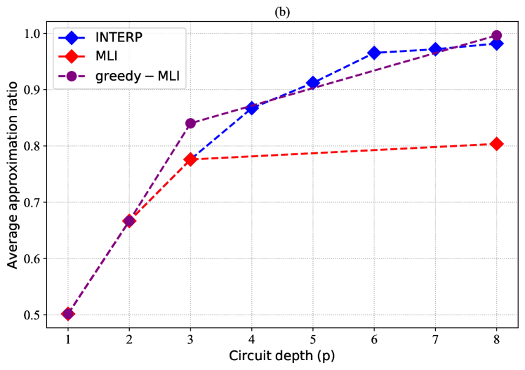
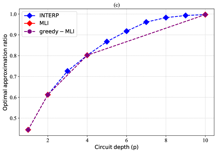
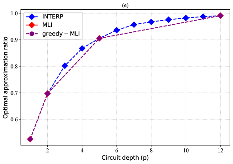
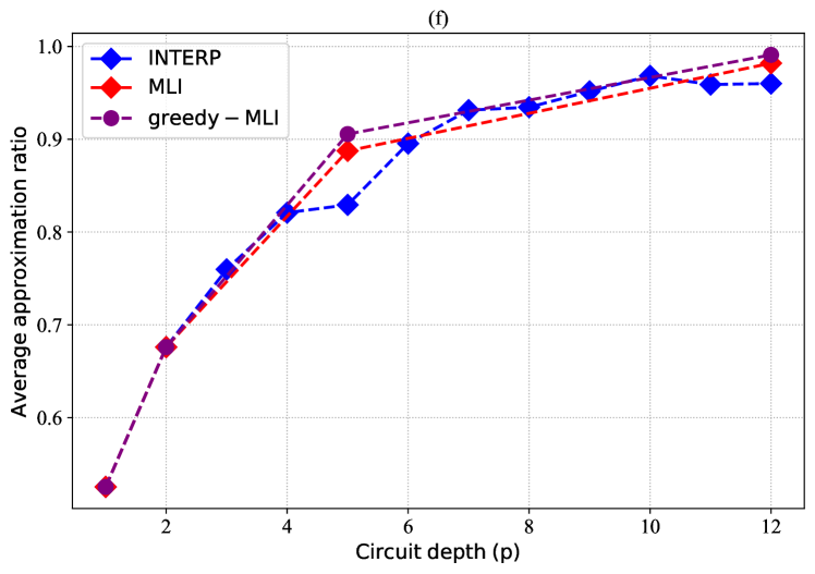
Figure 7: The performance comparison of three strategies on 3-regular graphs with vertex number $n=8,10,12$. Here, we take (a) and (b) as examples to analyze the simulation results. (a) MLI and greedy-MLI can obtain the same quasi-optimal value as INTERP in fewer rounds of optimization with $q=[1,2,3,8]$. (b) The average performance of greedy-MLI is better than INTERP and MLI at level $p=3$ ($p=8$), which benefits from discarding a part of low-quality optimized parameters for level $p=2$ ($p=3$).

IV Comparison among heuristics

We respectively generate 30 3-regular graphs for every vertex number $n$ to examine the difference in performance among heuristic strategies on the given graphs, where $n=8,10,12$. On each graph instance, we perform 500 optimization runs for INTERP and MLI, and one optimization run for greedy-MLI with $c=500$, where the target level equals the vertex number, and three initialization strategies start from the same initial parameters.

For our examples in figure 7, both MLI and greedy-MLI strategies work well for all the instances we examine. MLI and greedy-MLI achieve identical optimal performance as INTERP, but with significantly fewer rounds of optimization. This demonstrates that MLI and greedy-MLI are more efficient in reaching quasi-optimal solutions by skipping a substantial number of optimization rounds without sacrificing performance. The reduced computational overhead makes them promising alternatives for optimization tasks, especially for cases where computational resources are limited. Furthermore, we compare the average performance obtained by these strategies at the target level. Notably, we observed that greedy-MLI outperformed both INTERP and MLI in terms of average performance. This improvement is attributed to greedy-MLI discards a portion of low-quality optimized parameters during the optimization run. By doing so, greedy-MLI focuses on more promising parameter configurations, leading to better overall performance. The selective approach of greedy-MLI in parameter optimization provides a clear advantage over the other strategies, particularly when dealing with higher-level optimizations. This makes greedy-MLI well-suited for scenarios where computational resources are limited or when optimizing larger circuits with increased complexity.

To show the costs reduced by our strategies more intuitively, we independently calculated the running time of executing 500 optimization runs of MLI (or INTERP) and one optimization run of greedy-MLI, which can be seen in table 3. These results suggest that the running time reduced by MLI and greedy-MLI grows as the circuit depth increases, which benefits from reducing more rounds of optimization by increasing the depth step $l$. In addition, we find that the greedy-MLI strategy consumes the least amount of running time and achieves the best average performance.

Overall, the analysis of simulation results highlights the superiority of MLI and greedy-MLI over INTERP in terms of efficiency and performance. They not only achieve comparable quasi-optimal values with fewer optimization rounds but also demonstrate a higher average performance by discarding less promising parameter configurations. These findings underscore the effectiveness of multilevel leapfrogging initialization and the selective approach of greedy-MLI.

Table 3: The comparison of running time

$p$	INTERP	MLI	greedy-MLI
8	3119s	1432s	1199s
10	6589s	2398s	1512s
12	24720s	6761s	4070s

V Conclusion and outlook

In this paper, we present a novel approach called M-Leap for parameterized quantum circuits. The central idea behind M-Leap is to generate initial parameters for level $p+l$ leveraging the optimized parameters obtained at level $p$, a concept we refer to as multilevel leapfrogging initialization, which significantly reduces the number of optimization rounds required in the external loop optimization. Additionally, M-Leap also suits a broader class of problems, such as quantum circuit design, quantum circuit learning, quantum neural networks, and so on. It is interesting to explore the realistic performance of M-Leap on these training tasks.

Based on M-Leap, we propose two initialization strategies and explore their performance on the Maxcut problem. In the study of MLI, we focus on investigating the effects of $l$ on the performance of MLI. From the numerical results, we find that the performance of MLI may lower when $l$ surpasses $l^{*}$, which lies in lacking pre-information to generate good initial points. In addition, we conclude the regularities of the value of $l^{*}$ through numerous benchmarking. The obtained regularities can provide an initial conjecture of $q$ that allows MLI saves at least half of the optimization rounds, potentially making the classical outer learning loop of the quantum approximate optimization algorithm more simple and efficient. The simulation results show that MLI needs about $1/3$ of the cost of INTERP when it gets the quasi-optimal solution. The success of MLI and INTERP relies on the smooth parameter pattern. During simulations, we note that non-smooth parameters $(\bm{\gamma_{p}}^{n},\bm{\beta_{p}}^{n})$ may show the same optimal performance as smooth parameters $(\bm{\gamma_{p}}^{s},\bm{\beta_{p}}^{s})$. However, the performance of INTERP and MLI may deteriorate at level $p+1$ when they start from the initial points produced by non-smoothly optimized parameters $(\bm{\gamma_{p}}^{n},\bm{\beta_{p}}^{n})$. To overcome this shortcoming, we present greedy-MLI, which is an extension of MLI. To search for the smooth parameters during the optimization, greedy-MLI executes parallel optimization starting from $c$ pairs of initial parameters and only preserves the parameters with the highest approximation ratio after each round of optimization. The numerical simulations presented above suggest the better average performance of greedy-MLI, and it can get the quasi-optima consuming fewer costs compared with $c$ optimization runs of MLI or INTERP.

Reducing the training costs for parameterized quantum circuits in optimization tasks can accelerate the exploration of solution spaces and enhance the practicality of quantum optimization techniques. Under their efficiency, MLI and greedy-MLI can be as subroutines or preprocessing tools in other optimization algorithms in future studies. Although our heuristic initialization strategies show advantages in cost and performance for all 3-regular graph instances we examine compared with the existing work, the performance of MLI and greedy-MLI on other graph ensembles or optimization tasks (e.g., portfolio optimization, logistics planning, and supply chain management) is worthwhile to explore. Finally, we hope that the multilevel leapfrogging initialization established in this work can inspire future research that could lead to a better understanding of what happens under the hood of QAOA optimization.

References

- (1) Shor P W. Polynomial-time algorithms for prime factorization and discrete logarithms on a quantum computer. SIAM Journal on Computing, 1997, 26(5): 1484-1509.
- (2) Grover L K. A fast quantum mechanical algorithm for database search. In: Miller G L, eds. Proceedings of the STOC 1996. ACM, 1996. 212-219.
- (3) Harrow A W, Hassidim A, Lloyd S. Quantum algorithm for linear systems of equations. Phys. Rev. Lett., 2009, 103: 150502.
- (4) Lloyd S, Mohseni M, Rebentrost P. Quantum principal component analysis. Nature Physics, 2014, 10:631-633.
- (5) Wan L C, Yu C H, Pan S J, et al. Asymptotic quantum algorithm for the Toeplitz systems. Phys. Rev. A, 2018, 97: 062322.
- (6) Wan L C, Yu C H, Pan S J, et al. Block-encoding-based quantum algorithm for linear systems with displacement structures. Phys. Rev. A, 2021, 104: 062414.
- (7) Pan S J, Wan L C, Liu H L. Improved quantum algorithm for A-optimal projection. Phys. Rev. A, 2020, 102:052402.
- (8) Yu C H, Gao F, Wang Q L, et al. Quantum algorithm for association rules mining. Phys. Rev. A, 2016, 94(4): 042311.
- (9) Yu C H, Gao F, Liu C H, et al. Quantum algorithm for visual tracking. Phys. Rev. A, 2019, 99(2): 022301.
- (10) Yu C H, Gao F, Lin S, et al. Quantum data compression by principal component analysis. Quantum Information Processing, 2019, 18(249).
- (11) Yu C H, Gao F, Wen Q Y. An improved quantum algorithm for ridge regression. IEEE Transactions on Knowledge and Data Engineering, 2021, 33(3): 858-866.
- (12) Pan S J, Wan L C, Liu H L, et al. Improved quantum algorithm for A-optimal projection. Phys. Rev. A, 2020, 102(5): 052402.
- (13) Preskill J. Quantum Computing in the NISQ era and beyond. Quantum, 2018, 2:79.
- (14) Cerezo M, Arrasmith A, Babbush R, et al. Variational quantum algorithms. Nature Reviews Physics, 2021, 3: 625-644.
- (15) Bharti K, Cervera-Lierta A, Kyaw T H, et al. Noisy intermediate-scale quantum algorithms. Reviews of Modern Physics, 2022, 94: 015004.
- (16) Peruzzo A, McClean J, Shadbolt J, et al. A variational eigenvalue solver on a photonic quantum processor. Nature communications, 2014, 5: 1.
- (17) Grimsley H R, Economou S E, Barnes E, et al. An adaptive variational algorithm for exact molecular simulations on a quantum computer. Nature communications, 2019, 10: 1.
- (18) Grimsley H R, Barron G S, Barnes E, et al. Adaptive, problem-tailored variational quantum eigensolver mitigates rough parameter landscapes and barren plateaus. npj Quantum Information, 2023, 9: 19.
- (19) Du Y, Huang T, You S, et al. Quantum circuit architecture search for variational quantum algorithms. npj Quantum Information, 2022, 8: 62.
- (20) Tang H L, Shkolnikov V O, Barron G S, et al. qubit-adapt-vqe: An adaptive algorithm for constructing hardware-efficient ansatze on a quantum processor. PRX Quantum, 2021, 2: 020310.
- (21) Huang H Y, Bharti K, Rebentrost P. Near-term quantum algorithms for linear systems of equations with regression loss functions. New Journal of Physics, 2021, 23: 113021.
- (22) Bravo-Prieto C, Garcia-Martin D, Latorre J I. Quantum singular value decomposer. Phys. Rev. A, 2020, 101: 062310.
- (23) Cerezo M, Sharma K, Arrasmith A, et al. Variational quantum state eigensolver. npj Quantum Information, 2022, 8: 113.
- (24) Xu X, Sun J, Endo S, et al. Variational algorithms for linear algebra. Science Bulletin, 2021, 66: 2181-2188.
- (25) Bravo-Prieto C. Quantum autoencoders with enhanced data encoding. Machine Learning: Science and Technology, 2021, 2: 035028.
- (26) LaRose R, Tikku A, ONeel-Judy E, et al. Variational quantum state diagonalization. npj Quantum Information, 2019, 5: 57.
- (27) Lubasch M, Joo J, Moinier P, et al. Variational quantum algorithms for nonlinear problems. Phys. Rev. A, 2020, 101: 010301.
- (28) Liu H L, Wu Y S, Wan L C, et al. Variational quantum algorithm for the Poisson equation. Phys. Rev. A, 2021, 104: 022418.
- (29) Zhang S X, Wan Z Q, Lee C K, et al. Variational quantum-neural hybrid eigensolver. Phys. Rev. Lett., 2022, 128: 120502.
- (30) Wu Y, Wu B, Wang J, et al. Quantum Phase Recognition via Quantum Kernel Methods. Quantum, 2023, 7: 981.
- (31) Pan Y, Tong Y, Yang Y. Automatic depth optimization for a quantum approximate optimization algorithm. Phys. Rev. A, 2022, 105: 032433.
- (32) Zhang Y J, Mu X D, Liu X W, et al. Applying the quantum approximate optimization algorithm to the minimum vertex cover problem. Applied Soft Computing, 2022, 118: 108554.
- (33) Hadfield S, Wang Z, O’gorman B, et al. From the quantum approximate optimization algorithm to a quantum alternating operator ansatz. Algorithms, 2019, 12: 34.
- (34) Zhu L, Tang H L, Barron G S, et al. Adaptive quantum approximate optimization algorithm for solving combinatorial problems on a quantum computer. Phys. Rev. Research, 2022, 4: 033029.
- (35) Zhang B, Sone A, Zhuang Q. Quantum computational phase transition in combinatorial problems. npj Quantum Information, 2022, 8: 87.
- (36) Crooks G E. Performance of the quantum approximate optimization algorithm on the maximum cut problem. arXiv preprint arXiv:1811.08419, 2018.
- (37) Farhi E, Goldstone J, Gutmann S. A quantum approximate optimization algorithm. arXiv preprint arXiv:1411.4028, 2014.
- (38) Vikstal P, Gronkvist M, Svensson M, et al. Applying the quantum approximate optimization algorithm to the tail-assignment problem. Phys. Rev. Applied, 2020, 14: 034009.
- (39) Sack S H, Serbyn M. Quantum annealing initialization of the quantum approximate optimization algorithm. Quantum, 2021, 5: 491.
- (40) Streif M, Leib M. Training the quantum approximate optimization algorithm without access to a quantum processing unit. Quantum Science and Technology, 2020, 5: 034008.
- (41) Willsch M, Willsch D, Jin F, et al. Benchmarking the quantum approximate optimization algorithm. Quantum Information Processing, 2020, 19: 1-24.
- (42) Brandhofer S, Braun D, Dehn V, et al. Benchmarking the performance of portfolio optimization with QAOA. Quantum Information Processing, 2022, 22: 25.
- (43) Lee X, Xie N, Cai D, et al. A depth-progressive initialization strategy for quantum approximate optimization algorithm. Mathematics, 2023, 11: 2176.
- (44) Shaydulin R, Safro I, Larson J. Multistart methods for quantum approximate optimization[C]//2019 IEEE high performance extreme computing conference (HPEC). IEEE, 2019: 1-8.
- (45) Zhou L, Wang S T, Choi S, et al. Quantum approximate optimization algorithm: Performance, mechanism, and implementation on near-term devices. Phys. Rev. X, 2020, 10: 021067.
- (46) Alam M, Ash-Saki A, Ghosh S. Accelerating quantum approximate optimization algorithm using machine learning[C]//2020 Design, Automation and Test in Europe Conference and Exhibition (DATE). IEEE, 2020: 686-689.
- (47) Khairy S, Shaydulin R, Cincio L, et al. Learning to optimize variational quantum circuits to solve combinatorial problems[C]//Proceedings of the AAAI conference on artificial intelligence. 2020, 34(03): 2367-2375.
- (48) Moussa C, Wang H, Back T, et al. Unsupervised strategies for identifying optimal parameters in Quantum Approximate Optimization Algorithm. EPJ Quantum Technology, 2022, 9: 11.
- (49) Wauters M M, Panizon E, Mbeng G B, et al. Reinforcement-learning-assisted quantum optimization. Phys. Rev. Research, 2020, 2: 033446.
- (50) Brandao F G S L, Broughton M, Farhi E, et al. For fixed control parameters the quantum approximate optimization algorithm’s objective function value concentrates for typical instances. arXiv preprint arXiv:1812.04170, 2018.
- (51) Lee X, Saito Y, Cai D, et al. Parameters fixing strategy for quantum approximate optimization algorithm[C]//2021 IEEE international conference on quantum computing and engineering (QCE). IEEE, 2021: 10-16.
- (52) Wurtz J, Lykov D. Fixed-angle conjectures for the quantum approximate optimization algorithm on regular MaxCut graphs. Phys. Rev. A, 2021, 104: 052419.
- (53) Karp R M. Reducibility among combinatorial problems. Springer Berlin Heidelberg, 2010.
- (54) Wurtz J, Love P. MaxCut quantum approximate optimization algorithm performance guarantees for p¿ 1. Phys. Rev. A, 2021, 103: 042612.
- (55) Albash T, Lidar D A. Adiabatic quantum computation. Reviews of Modern Physics, 2018, 90: 015002.
- (56) Skolik A, McClean J R, Mohseni M, et al. Layerwise learning for quantum neural networks. Quantum Machine Intelligence, 2021, 3: 1-11.
- (57) Sack S H, Medina R A, Kueng R, et al. Recursive greedy initialization of the quantum approximate optimization algorithm with guaranteed improvement. Phys. Rev. A, 2023, 107: 062404.
- (58) Akshay V, Rabinovich D, Campos E, et al. Parameter concentrations in quantum approximate optimization. Phys. Rev. A, 2021, 104: L010401.
- (59) Xie N, Lee X, Cai D, et al. Quantum Approximate Optimization Algorithm Parameter Prediction Using a Convolutional Neural Network. arXiv preprint arXiv:2211.09513, 2022.
- (60) Mitarai K, Negoro M, Kitagawa M, et al. Quantum circuit learning. Phys. Rev. A, 2018, 98: 032309.
- (61) Zhu D, Linke N M, Benedetti M, et al. Training of quantum circuits on a hybrid quantum computer. Science advances, 2019, 5: eaaw9918.