A Computational Theory and Semi-Supervised Algorithm for Clustering

Abstract

A computational theory for clustering and a semi-supervised clustering algorithm is presented. Clustering is defined to be the obtainment of groupings of data such that each group contains no anomalies with respect to a chosen grouping principle and measure; all other examples are considered to be fringe points, isolated anomalies, anomalous clusters or unknown clusters. More precisely, after appropriate modelling under the assumption of uniform random distribution, any example whose expectation of occurrence is $<1$ with respect to a group is considered an anomaly; otherwise it is assigned a membership of that group. Thus, clustering is conceived as the dual of anomaly detection. The representation of data is taken to be the Euclidean distance of a point to a cluster median. This is due to the robustness properties of the median to outliers, its approximate location of centrality and so that decision boundaries are general purpose. The kernel of the clustering method is Mohammad’s anomaly detection algorithm, resulting in a parameter-free, fast, and efficient clustering algorithm. Acknowledging that clustering is an interactive and iterative process, the algorithm relies on a small fraction of known relationships between examples. These relationships serve as seeds to define the user’s objectives and guide the clustering process. The algorithm then expands the clusters accordingly, leaving the remaining examples for exploration and subsequent iterations. Results are presented on synthetic and realworld data sets, demonstrating the advantages over the most widely used clustering methods.

1 Introduction

Grouping is a natural process carried out by humans in their interaction with the environment and is particularly considered fundamental when interpreting and understanding visual information. This is exemplified in the theories of human vision, and in particular the Gestalt Theory of Psychology where partial gestalts (local groupings) are taken to repeatedly fuse to culminate in global perceptions [2]. It is thus natural to see that grouping—otherwise known as cluster analysis in the field of machine learning—is ubiquitous and appears in practically all disciplines where data is collected. This includes malware clustering in cybersecurity, topic clustering in document processing, fraud analysis in finance and grouping gene expressions in molecular biology. The wide range of subjects highlights the importance of cluster analysis; specifically for the exploration, representation and understanding patterns of interest.

However, clustering data into meaningful groups is a challenging problem. Not least because even defining and framing the problem so as to state precisely what is to be computed is fraught with difficulties. Often the problem is vaguely posed as finding natural groupings of the data where within group points are similar with respect to some measure like distance, density or probability, yet dissimilar from other such formations. However, the problem statement also needs to make explicit that some observations may be noise or anomalies and not belong to any meaningful group, or be altogether a completely unknown group, thus requiring more nuanced decision boundaries and not the forceful lumping of all examples into some groups.

Another factor that leads to challenges is the type of learning encountered in cluster analysis—machine learning algorithms generally fall under the categories of supervised, unsupervised and semi-supervised. In supervised learning labels of the data are all available and the goal may be to learn a classifier or a predictor. In unsupervised learning data is unlabelled and is a scenario most widely encountered in the realworld because most data is unlabelled and acquiring such labels can be costly (or even unnecessary). The term unsupervised is also often interpreted to mean that the algorithms run without user assistence and interaction; here an algorithm returns what it deems to be the best result, or a number of different results are made available for the user to select according to their goal. The semi-supervised learning category normally assumes that some small fraction of labelled data is available, or only the labels of a particular class; such information can help guide, validate and improve the methods.

The cluster analysis problem usually falls under the category of unsupervised learning and is used to find patterns of interest; however, deciding what is the ideal way to formulate and guide (optimisation) algorithms is difficult, as well as the measuring of performance. This has resulted in many heuristic based algorithms for which users are left to supply critical parameters that cannot be automatically reliably inferred from the data. Instead, such parameters may be estimated by data exploration, visualisation, sampling and labelling. Thus, it seems reasonable to question whether these algorithms are truly unsupervised; instead placing them into the category of semi-supervised learning where even though labelled data is not used at the outset, the user is providing some additional information to the algorithm that is obtained through human intuition and experience of the specific data or domain. Interestingly, such information can often be interpreted as constraints on the possible data partitions or clusters that can be returned by the algorithm, where the parameters specify the resolution at which the process is to be carried out.

In more recent years clustering has also become explicitly semi-supervised through the ideas of constrained clustering where typically samples of labelled data or relationships are leveraged in some modified version of the $k$-means algorithm [10]. This form of clustering is practical and interactive since in many scenarios some data or knowledge of clusters is available and supervision can take the goals of the user into consideration at multiple steps. Furthermore, this specification of constraints for clustering is important because without guidance or additional external information (that is unavailable from the data), the algorithm cannot know the criteria by which to cluster, nor the level of resolution that is commensurate with the goal.

In the present work both the unsupervised and semi-supervised approaches to clustering are of interest—leaving aside a strict definition. The former has benefits of ease of use while the latter can use explicit prior information from the user to guide or constrain the clustering to solutions that are desired amongst the vast number of possibilities.

1.1 Prior Art

There are several general approaches in unsupervised clustering which include hierarchical, density, spectral, information-theoretic, probability and distance to the centroid based methods. For each approach, together with a representation of the data, many algorithms have been developed that are usually modifications of the fundamental idea so that certain deficiencies are claimed to be overcome. However, this normally introduces complexities that result in an overall less practical algorithm in terms of additional runtime, storage or parameters. It is thus important to note that even with the flux of new algorithms over the past decades, the most widely used and cited algorithms are still agglomerative clustering, DBSCAN, gaussian mixtures and $k$-means.

No single algorithm can work best across all data sets and for every data set that an algorithm particularly excels at one can construct another where it fails. However, there are still properties an algorithm may have that are generally problematic. These include: the setting of unintuitive and data specific parameters that can be nigh on impossible to specify in advance and difficult to do so even after data exploration; high runtime and storage requirements with increasing number of observations or dimension of the data; the assignment of anomalies to a cluster when they are clearly alien to the group; the inability to predict on new data points given the current clustering; and being unable to produce good clustering results across as many varieties of data sets and domains actually encountered in the realworld as possible.

For example, in hierarchical clustering such as the agglomerative method [11], users are required to specify the granularity at which clusters are to be taken. This has the advantage that clustering can be considered at different resolutions or levels but requires nontrivial (and perhaps unintuitive) specification on the users part. There are also a number of linkage methods to select from that can give different results. The runtime of the algorithms and storage requirements are also prohibitively expensive with increasing number of examples; being $O(n^{2}logn)$ and $O(n^{2})$, respectively. Another important aspect to note is that all merges are final in the building of clusters. This can be problematic when for example there are anomalies present since the grouping cannot adjust or correct later to a better solution. Furthermore, the hierarchical method does not natively associate a score with an observation or predict the cluster label of a new observation given the current clustering, this restricts its utility somewhat unless additional classifiers are applied on top.

Density based methods work on the premise that clustering locates regions of high density that are separated from one another by regions of low density. The most popular method is DBSCAN [3] which can cluster arbitrarily shaped data distributions efficiently ($O(nlogn)$ runtime and in $O(n)$ memory), while also potentially detecting anomalies. However, it requires the specification of parameters that are highly sensitive and difficult to set in practice even with the ‘elbow’ identification method. Thus, it can fail to give good results in even what appear to be simple data sets if clusters are too close to one another or there are large differences in densities. The method also benefits from post-processing to remove small groups of data that may get incorrectly classed as clusters, and it has been found in private experiments that its anomaly detection results are unsatisfactory. DBSCAN also does not natively provide a cluster association score for every observation or have predictive ability over new observations. The only way to handle the latter issue is to rerun the clustering again with the new data.

Probability based models fit statistical models to the data and estimate parameters, with the mixture of gaussians method being the most popular. In the cases where the assumptions are met it can give very good results, and the data points are not only assigned a grouping but each also has an associated probability score of belonging. The use of distributions enables simple characterisation of the clusters produced by the parameters, and has some general applicability in terms of handling ellipsoidal clusters. However, the method can be particularly slow due to the use of the Expectation Maximisation algorithm for finding the distribution parameters and hence is not practical for large data sets. It also does not work well when there is little data, if the data points are nearly co-linear, when the number of groups is assumed incorrectly, or when the gaussian data distribution assumption is not met. Noise and anomalies are also not natively handled since it computes a partitioning.

Of all the clustering algorithms mentioned thus far, it is still the simple method of $k$-means [5, 4] that is the most widely known and stands out as the algorithm of choice for practitioners—despite it being over $50$ years old. It does however have several drawbacks which has resulted in much additional development, but most of which have not gained traction for practical use because of the additional complexities they introduce without necessarily better results. Due to it being a centroid based method, and because of its widespread appeal and use, comparisons in the present paper will focus more on $k$-means since any algorithm that can better or complement it will be a significant contribution to the field of cluster analysis. Hence, this algorithm will be elaborated upon.

$k$-means has a number of important properties that have made it popular. Foremost is its simplicity to understand and to implement, and it is very fast to compute in practice—both with increasing feature dimensions and the number of examples. Its time complexity is $O(tknd)$ ($t$: number of rounds, $k$: number of clusters, $n$: number of observations, $d$: dimension of data) and so it is linear with the number of examples in the data. It’s speed also makes it suitable for interactive use which is important for exploratory work. The space complexity is also low, being $O((n+k)d)$. $k$-means being a centroid based method also benefits from being able to natively score points and predict upon new data by simply using the distance to the centroid of the parent cluster; both of which can be beneficial in applications. Like other algorithms it requires parameters, principally the value $k$ specifying how many clusters the algorithm is to return. Indeed, too few will result in some groups being clumped together as one, while too many will result in desired clusters being separated into sub-clusters. However, users can intuitively understand this parameter and in specific problems are able to set it in advance, estimate it using the ‘elbow’ method or gauge it interactively from the clustering results. Thus, although the ideal solution is parameter-free, having only a single intuitive parameter alleviates the burden somewhat and makes $k$-means appear relatively straightforward to use compared to other algorithms.

However, $k$-means is sensitive to the initialisation centroids, resulting in getting stuck in local optima so that multiple runs with random initialisation is sometimes recommended. However, this may not necessarily work well depending on the data and number of clusters specified. Thus, another approach includes taking samples of points and clustering them using hierarchical clustering where the centroids of those clusters are used as seeds. This approach may only work well if the sample size is small due to the computational complexity of hierarchical clustering and if $k$ is relatively small compared to the sample size. Note that the number of clusters still requires specification and its empirical success remains unclear. Other extensions include $k$-means$++$ and bisecting $k$-means. The former picks centroids incrementally where new centroids are taken to be a random one that is far from its closest centroid and based on a probability measure that is proportional to the square of its distance. The latter splits the data into two clusters, and repeatedly operates on one of the clusters until $k$ clusters have been produced. Interestingly this method also yields a hierarchical clustering by recording the sequence of clusterings produced as $k$-means bisects each cluster.

The optimisation criteria and the computation of centroids using local means makes $k$-means sensitive to anomalies which can lead to suboptimal partitions of the data. However, detecting and removing anomalies first is a challenging problem in of itself. In the case of clustering followed by anomaly removal, the sequential combination requires further analysis and practical investigation due to the distorting affect anomalies can have on the initial clustering. Another couple of methods similar to $k$-means, called $k$-medoids and $k$-medians have been proposed to overcome the problem of sensitivity to anomalies. The former takes an actual point to represent a cluster rather than the mean, while the latter uses medians as representatives. However, both are generally computationally slower than $k$-means, particularly when the data set and $k$ are very large.

Closely related to the problem of anomalies is that $k$-means can give undesirable partitions in the presence of clusters with different sizes or densities. Additionally, because it is a partitioning algorithm it will always place an example into a cluster even if it is an anomaly, a cluster of anomalies or in fact belongs to another unknown cluster. Thus, it is important to differentiate between algorithms that return clusters (such as DBSCAN) and partitioning algorithms since the term clustering is overloaded. It is usually the case that when users want to carry out cluster analysis, they desire groups of data that are similar to be returned while excluding that which does not belong to the group. This has implications with regard to what should be computed in the problem of clustering data and whether $k$-means is merely approximating what is desired of an algorithm.

A criticism often levied at $k$-means is its inability to cluster certain complex grouped data since it constructs hyperspherical clusters (or hyperellipsoidal clusters when using the Mahalanobis distance). While this is a point of criticism, it may in fact be a contributing factor for its widespread and general use since it does not follow the detailed distribution of the data and potentially suffer from overfitting. Indeed, it is assumed in this paper that for many realworld data sets, desired cluster groupings are roughly hyperspherical or are separate enough that such a clustering assumption works well in practice.

$k$-means has also been the basis of many semi-supervised clustering algorithms, with perhaps the most well known of them being $COPK$-means [10] and $PCK$-means [1]. The former operates by assimilating hard constraints from the user that cannot be violated while carrying out $k$-means clustering. Thus, the constraint labelling is assumed noiseless. Similarly, the latter method incorporates constraints from the user, but these are soft constraints where the algorithm suffers a penalty for violation. Both algorithms have claimed to improve clustering results over the standard unsupervised version. However, although the application domain is important (since oftentimes some labelled data or constraints are available), these methods have received little attention in practice. This is perhaps because the data sets used in the original works are relatively small, the algorithms slower to run, and because the results are not substantially improved. Furthermore—if it is of concern—most of the practical drawbacks of the $k$-means algorithm are also carried over into these semi-supervised implementations.

1.2 Contributions

Data clustering is intended to be carried out by a computer due to the size, number, diversity and speed at which information needs to be processed. However, oftentimes there is a comparison with the human ability to cluster sensory stimuli or data (particularly in low dimensions) which is carried out innately and effortlessly. Thus, to reach an ideal solution it seems pertinent to understand and learn from how humans might address or even solve the problem—particularly the diversity aspect and speed at which it is conducted.

Our starting point will be to consider clustering systematically as an information processing task and addressing it using David Marr’s [6] three levels of analysis—particularly the computational theory and algorithmic levels. This approach disciplines us to ask the correct questions at the appropriate levels of explanation so that we can better understand the overall task. Thus, beginning with the top level of computation we can ask in general and precise terms what is to be computed—the inputs and outputs—and why it is appropriate, and what realworld constraints should be incorporated to make clustering tractable. Then we can consider the next level of processing to derive representations of the data examples, the inputs and outputs, the nature of the ill-posed problem, and how we might bring in additional assumptions to develop an algorithm for carrying out the transformation from input to the desired output.

The present work builds a clustering algorithm from the ground up by following the above analyses and using human visual perception as inspiration. This approach was successfully used by Mohammad [8] in his development of anomaly detection, which will form a core component of the clustering method. Indeed, clustering is considered the complement of anomaly detection (sensing distinctness), where clusters are deemed to be sets of data points that do not contain any anomalies with respect to a chosen grouping principle and measure. Mohammad’s definition of an anomaly is used, and data points are represented as the distance to the median of the parent group so that hyperspherical clusters are formed in order to have a solution that is generally applicable and practically useful like the $k$-means algorithm (while accepting failure in other and non-hyperspherical distributions). Furthermore, anomaly detection being the core of the approach naturally results in isolated points or clusters being labelled as anomalies so that clustering—and not a partitioning of the data—is carried out.

Note that clustering is done to discover meaningful groupings of the data or interesting patterns that may not have been previously known. However, without embedding or conveying to an algorithm what is desired or considered meaningful, an algorithm cannot know which grouping of the data is appropriate. Indeed, any random clustering could be returned and justifiably so since constraints or requirements have not been provided. This resonates with the idea from human vision studies that intelligence identifies the appropriate resolution for the present utility, with perception iconicising the visual input at that appropriate level. Most algorithms implicitly assume some desired properties of the clusters in addition to requiring parameters, these naturally constrain the possible solutions. In the case of $k$-means it is that clusters are hyperspherical in nature and of similar size and density, and the data is without noise or anomalies, with a specified number of clusters; the computational problem being to minimise the within partition sum of squared error. While for DBSCAN regions of high density are considered clusters where the output is constrained by the two parameters specifying a radius to compute densities and the minimum number of points to be in that region. In the semi-supervised algorithms such as $COPK$-means, the base $k$-means assumptions are held, and in addition the labelled examples or pairwise constraints are provided to help the clustering approach the users desired outcome.

The clustering method presented in this paper is parameter-free but assumes an interactive process between human and machine, where users must provide a small amount of labelled data that approaches a constant with increasing size of the data per cluster, so that seed members of known groups are obtained. This little information is enough to constrain and guide the algorithm to grow meaningful clusters and carry out both local and global anomaly detection. As users interact with the clustering outputs, further observations can be sampled, analysed and discovered, while existing clusters may be modified. The method—being based on Mohammad’s anomaly detection algorithm—is fast, intuitive and light on memory usage. Furthermore, because there is no best clustering algorithm in general, a framework is also provided (but not yet developed) for dealing with other useful representations of data in order to tackle different data distributions.

To detail the contributions of this work, the rest of the paper is laid out as follows: Section 2 provides a computational theory of clustering and describes the parameter-free, semi-supervised clustering algorithm. Section 3 gives some empirical results on synthetic one-dimensional and two-dimensional data sets to intuitively understand the performance of the algorithm. Additional results on publicly available data sets are also provided to demonstrate realworld applications. Finally, section 4 concludes the paper and provides some thoughts for future work.

2 A Computational Theory for Clustering

The goal of the present work is to draw insights from the human visual process of object grouping and develop an algorithm capable of automating clustering tasks on large datasets. In the case of complete automation we will have an unsupervised solution, whereas when we permit a small amount of human involvement (labelling data) or interaction (iterative evaluation) we will have a semi-supervised solution.

Human vision is considered to be an example of complex information processing for which Marr [6] introduced the idea of a three level analysis. His core theme was that vision is not governed by a single explanation, equation or level of understanding, but that each visual task requires its own multiple levels of analysis which form a top-down hierarchy. This approach has significantly impacted the field of computational neuroscience because it helps delineate what is to be computed and whether it satisfies assumptions obtained from the realworld and with what is desired of the task, from how one might carry out the computation and its implementation. This section will describe the levels of analysis as applied to the problem of clustering, and present an algorithm for efficient computation.

2.1 Tri-level Hypothesis

The top level in Marr’s analysis is called the computational level and deals with what the computation is, or the goal of the task, and why it is appropriate; this is interpreted at both the general and specific levels. At the general level we answer what information is extracted and why it is useful, while at the specific level we state exactly what is to be computed from input to output and what realworld constraints or assumptions are generally true of the world and powerful enough, to allow a process to be defined and the desired outcome to be achieved. The constraints help decide whether the actual function is the one that should be computed, and why this computation is specified instead of some other for the task at hand. Finding such constraints that impose themselves naturally to sufficiently allow a unique solution is a true discovery of permanent value even if it is not internally verifiable.

The second level in the analysis is the algorithmic level and is concerned with how the computations associated with the first level are to be carried out. This is broken into two parts. First is the specification and representation of the data input and output, and second is the actual algorithm that carries out the transformation. Note that many representations can be put forward, and each can make some aspects explicit and relegate others to the background—this has significant bearing on the choice of algorithm. Indeed, for each representation many algorithms can be chosen and each algorithm may have certain desirable and undesirable characteristics according to the specific problem.

The third level of analysis, known as the implementation level, focuses on the physical realisation of the computations. This can involve various systems, ranging from the human brain to specialized mechanical machines, but for our purposes it will be a single computer. Nevertheless, it may be important to consider the potential extensions to distributed implementations in scenarios such as big data applications and distributed devices.

2.2 Computational Theory

The clustering problem is generally understood to be the grouping of portions of data that are similar in a particular way, but separate from other such groups. The process has important applications in data mining where the output can be used—amongst other purposes—for segmentation, summarisation and classification. The input to the problem is assumed to be in a dataframe format, where examples are represented as rows and feature values as columns of numbers. The desired output is a one-dimensional array of labels that identify which cluster each example belongs to and in addition there may be a membership score. Note that a specific cluster label is required for the unknown or anomalous group. Unfortunately, there is not enough information available in the input to get a unique desired output directly and hence any partitioning of the data could be returned. The problem is ill-posed, and we require additional external information to constrain the possible solutions; we derive this from the human experience of grouping data points in low dimensisonal spaces.

The process of clustering is distinct from partitioning; subsets of data points may be grouped into a cluster but not necessarily all points should be assigned to a cluster. This then provides our first natural and most important constraint that similar points should be clustered together, but anomalies with respect to every grouping and measure, must not belong to any cluster. The second assumption is that an object that is part of a cluster has both a membership and degree of membership. In other words even within a single group all observations have a level of belonging. For example, points that are further away from the centroid or occupy less dense regions of space than others.

The removal of what is anomalous—with respect to some characteristic—from a set of data points, leaves us with a group of points that are now deemed similar; hence, the following definition of a cluster is made:

Definition 2.1 (Cluster).

A cluster is a subset of data points that does not contain any anomalies with respect to a chosen grouping principle and measure.

This definition needs to be made precise and requires some additional explanation and support. Assuming that the realworld physically imposes natural groupings of interest, the term anomaly is taken to be that defined by Mohammad [8].

Definition 2.2 (Anomaly).

A grouping of interest represented by a gestalt law is perceived by the Helmholtz principle when it is unexpected to happen (i.e. its expectation of occurrence is $<1$) in uniform random noise. Any observation that is unexpected to occur with respect to this grouping is perceived, by the same principle, to be an anomaly.

Anomalies, according to this definition can be computed precisely, and an algorithm under a particular representation of Euclidean distance from the median is provided by Mohammad [8]. This not only provides us with a classification but also a score defining the degree of anomalousness. Hence, clusters being simply the complement of the set of anomalies in the data are also computable and have an associated score. This also satisfies a third constraint that is taken as an assumption: what is computed must have parameters or thresholds that adapt to the data, and are not fixed unless they are universally useable. This is reasonable to assume since data sets, and indeed clusters within data sets, can vary in terms of numbers, size, density or shape and an algorithm needs to be able to best adapt to such differences. However, the constraint is unlikely to be universally satisfied across all data sets due to the range of possible data distributions and the specificity of each adaptation.

The clustering process is approached from the perspective of removing anomalies as it provides a more intuitive and appreciable framework. This viewpoint allows for easier understanding and handling of the subject and algorithms, emphasising that points classified as not belonging to any group are considered anomalies.

Gestalt groupings play an important role since clustering is often described as finding natural groupings in the data. (Figure 1 illustrates some examples of ‘natural’ clusters by proximity.) Thus, it can be argued that satisfactory clustering results are not completely aribtrary, in that though a staggeringly large number of possible cluster outputs can be returned, it is only a relative few that are acceptable. Thus, the groupings that we care about and consider natural are limited and are conjectured to include grouping by the gestalt laws such as proximity, good continuity and similarity. These groupings should agree with what the common man sees and believes to be true. Clustering is in the eye of the beholder is an old adage, but the eye being human is constrained by only perceiving certain patterns that correspond to prior grouping laws of interest.

2.3 Representation

There are many ways in which humans group things, and how things can be represented. For example, there is grouping by shape, size, continuity, distance between objects, colour and any combination of these. Thus, the clustering problem also requires users to specify the goal by which data points are desired to be grouped by, and it is only the grouping that has some utility that is desired. It is assumed that clustering is an interactive process in that a user does not simply run an algorithm and take the output at face value. Rather, checks are carried out, samples of clusters are taken, and the results are intuitively checked for consistency and the data explored further. Hence, the information by which the grouping is desired is obtained by the assumption that a user is able to provide cluster labels to a tiny fraction of the data in order to seed the required goals of the clustering. (This is perhaps akin to how a child may view some unknown objects and is then provided only a handful of labelled examples from which it is able to extrapolate and learn the abstract class.) Note that together with the exclusion of anomalies from a group, and the labelling of some data points that belong to a group from which clusters can be grown, another constraint is realised: unknown clusters of data that have no samples of labels should not be incorrectly assigned a cluster label of another group. Unknown groups here should simply be highlighted as anomalies with respect to all other groupings, and require uncovering through the users iterative and interactive exploration and labelling of the data.

Although it may appear that requesting users to supply similar examples is difficult, any clustering algorithm output necessarily requires that the user evaluate the results by looking at samples from the cluster to ascertain whether meaningful groupings have been obtained. This necessarily requires that the user has some domain expertise or knowledge of the features. This part of the evaluation is brought forward so that users are asked in advance to provide a small number of examples that likely belong to the same cluster. The labelling does not have to be comprehensive or completely accurate, since toleration of a minority of mislabelled examples is handled by the ejection of anomalies.

For a given representation of the data points, certain groupings of interest are highlighted, and others are hidden. The representations often used in cluster analysis include distance from the centroid, density within a radius of a point or distance between two examples. (Note even the notion of distance between two points can be broken down into further subgroups like Euclidean, Manhattan or Mahalanobis). Thus, another constraint that is selected by the user is the choice of representation and measure. For the purposes of clustering in this paper, it is assumed that the Euclidean distance to the centroid (median) of a cluster is an appropriate measure by which data points are to be grouped, or equivalently anomalies removed from the set to leave a grouping. This is because it is assumed data is often transformed such that the Euclidean distance works well and is one of the reasons why $k$-means has wide and general applicability. Furthermore, there is no evidence that another metric is better in general. The median is the chosen centroid instead of the mean because of its robustness to extreme deviations and better measure of central tendency.

Other measures related to grouping laws such as density, good continuity, repetition, etc. are also of importance and may be preferred in certain applications. In such cases a grouping of the data must be chosen. For example, a plane of best fit may be selected if the grouping of interest is best described by good continuity, hence any examples that deviate by an unexpected amount would be deemed anomalous with respect to the group.

2.4 Algorithm

Given a representation of the data points—which is defined as the Euclidean distance from the associated median—and a small subsample of labelled data, this section presents an algorithm for transforming the input into the desired output. The primary computational task involves detecting and removing anomalies from a set of data points, while simultaneously expanding clusters by incorporating non-anomalous points. Thus, anomaly detection lies at the core of the philosophy and method employed.

Here, we also acknowledge an additional constraint arising from the human ability to quickly perceive clusters in low-dimensional data, as well as the requirement to efficiently compute clusters over large realworld datasets. Namely, that the developed algorithm must be fast to compute and scale efficiently with increasing numbers of examples and dimensions of the data. Many clustering algorithms that yield satisfactory results with small datasets or low-dimensional data often struggle to meet these requirements, resulting in unacceptably long computation times.

To begin with, the clustering process requires users to provide a small subsample of known cluster assignments, possibly obtained randomly, that are largely accurate. These assignments serve as the initial seeds and guides for the clustering, while all other points are initially considered anomalies. Subsequently, the algorithm iterates over the clusters in order of the tightest concentration of points. For each cluster, anomalies are identified and ejected from the cluster, being reassigned to the anomaly category. Following this step, the algorithm examines all the anomalous points to determine if they should be considered anomalies or potentially belong to the cluster. Points that are determined to be non-anomalous have their label assignments changed to match the current cluster, while the labels of anomalies remain unchanged. This process of ejecting anomalies and expanding clusters continues iteratively until no further changes in the clustering occur or a maximum number of iterations have completed. The algorithm’s pseudocode is given below where Mohammad’s anomaly detection algorithm, called Perception, is used to detect anomalies parameter-free:

Input : Data points, subsample of labeled data, $max\_n\_iterations=1000$

Output : Cluster labels and membership score

Initialisation : 

1Initialise all unlabelled points as anomalies with label $-1$;

2 Order the labelled cluster groups by minimum sum of squared error;

3 $counter=0$;

4

5while cluster changes occur and $counter<\text{max\_n\_iterations}$ do

6       foreach cluster do

             // Fit anomaly detector and check for anomalies:

7             $clf=\text{Perception()}$ ;

8             $clf.fit(\text{cluster})$;

9             $clf.predict(\text{cluster})$;

10             if anomalies are found then

11                   Remove anomalies from the cluster and assign them to the anomaly category;

12                  

13             end if

            // Re-fit classifier on cluster without anomalies:

14             $clf.fit(\text{cluster})$;

             // Examine all anomalous points:

15             foreach anomalous point do

16                   prediction, score = $clf.predict(\text{$anomalous\ point$})$;

17                   if prediction is non-anomalous then

18                         Change point label assignment to match the current cluster;

19                        

20                   end if

21                  else

22                         Leave anomaly label unchanged;

23                        

24                   end if

25                  

26             end foreach

27            

28       end foreach

29      $counter=counter+1$;

30      

31 end while

32

33Re-fit the Perception() model on each cluster and compute scores;

34 return labels and membership scores of all examples;

Algorithm 1 Semi-supervised clustering

3 Experimental Results

This section provides the results of the clustering algorithm over several data sets. This includes one-dimensional and two-dimensional synthetic data, and then a selection of publicly available data sets. Although the presented method is semi-supervised, comparisons are not made against COPK-means or PCK-means. This is because their results were remarkably similar to standard $k$-means, but with longer execution times and the need for additional constraints. Instead, comparisons are made with $k$-means (with the given $k$ used where possible) and DBSCAN ($mps$ and $eps$ decided as in the guidelines of the original paper). The implementation of these algorithms is done using the scikit-learn library [9]. These algorithms were chosen due to their widespread appeal and usage when users encounter clustering problems, aiming to demonstrate the effectiveness of our proposed method.

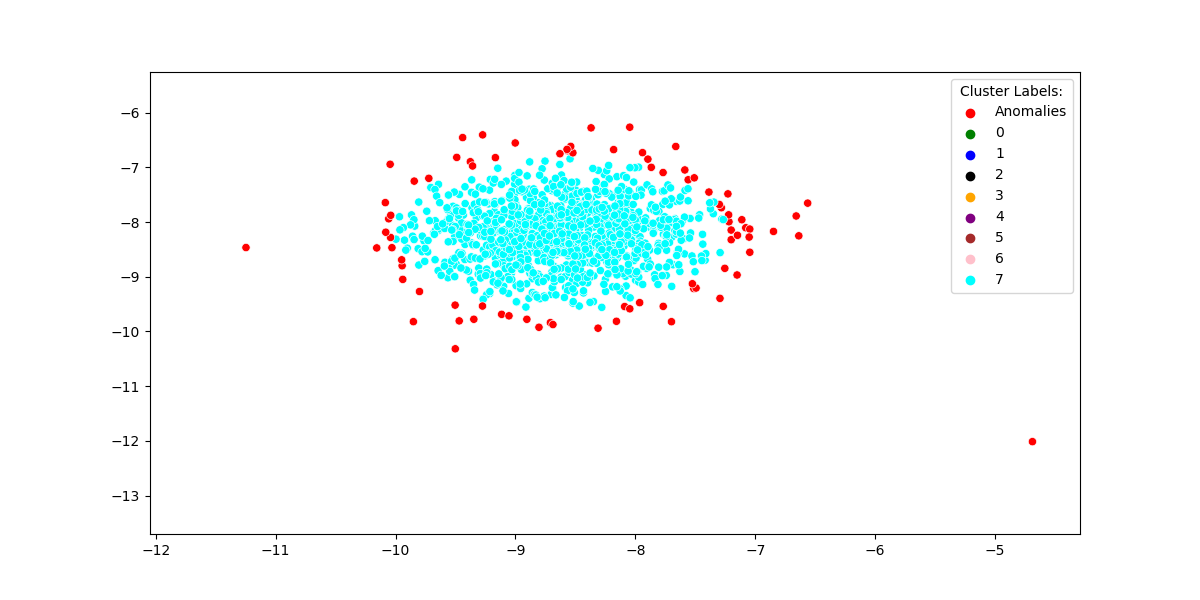
Evaluation of clustering algorithms is notoriously difficult because of the large number of measures from which to choose, and because certain measures favour certain algorithms due to the nature of the optimisation problem being solved. Partioning algorithms will also give very different results to clustering algorithms that report anomalies (such as the one presented in this paper), and may also appear artificially superior. This is because many data sets assign all examples to some cluster, and do not highlight those that are actually anomalies. Hence, even the ground truth labelling may not always be an accurate reflection of reality; for example in the generation of gaussian clusters it can be argued that there are outlying points with respect to the central mass of points of each cluster (e.g., Figure 9). In addition, it is important to consider that a dataset can be clustered in multiple ways or based on different features. Therefore, even with the availability of labels for evaluation, a clustering method may produce valid and effective clusters but which do not align with the pre-existing labels. Consequently, this work adopts a qualitative approach to address the clustering evaluation problem.

3.1 One-dimensional Synthetic Data

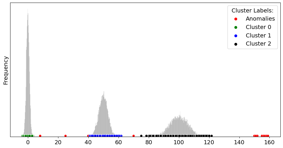
The first data set presented is composed of three gaussian distributed clusters, each of size $10000$ examples with centers $[0,50,100]$ and standard deviations of $[1,3,6]$. Added to this set are a few additional isolated local anomalies, a few mislabelled examples, and a small globally anomalous cluster. Figure 1 illustrates the data distribution where each of the three clusters are labelled and coloured—black, blue and green—and anomalies shown in red. Note however that anomalies resulting from the generating gaussian distribution for each of the clusters are not highlighted as such since it would require selecting an anomaly detection algorithm which may give results different to another, and that such algorithms often require appropriate but unknown parameters. In addition to the labelled scatter plot, a histogram is also provided to show the relative densities which is otherwise hidden in the plot.

Figure 1: Three labeled gaussian distributed clusters with a few additional mislabelled examples, some isolated anomalies and a small anomalous cluster.

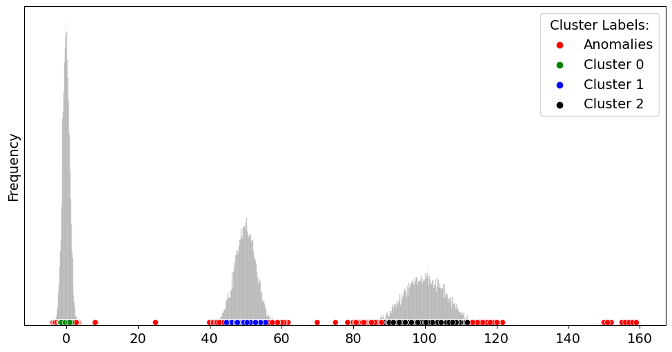
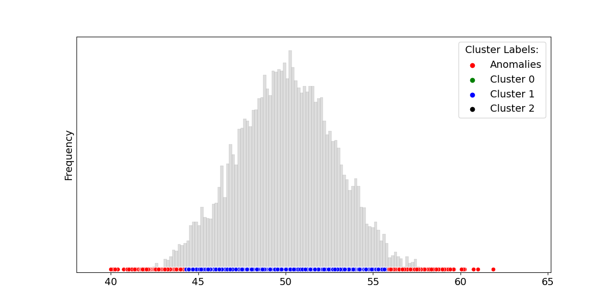
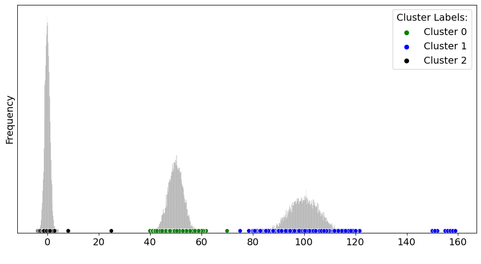
A tiny fraction of the data—approximately $150$ examples ($0.5\%$) together with their labels—are randomly chosen from the data (excluding the small anomalous cluster). These labels act as the seeds for the proposed semi-supervised clustering algorithm and are expected to have been provided by the user after familiarising themselves and interacting with the data and domain. Note that the seeds need not cover all clusters since unrecognised clusters will simply be reported as anomalies and can be analysed in subsequent rounds. The results of the algorithm are shown in Figure 2 where three clusters are identified along with the isolated anomalies and small anomalous cluster; the latter of which can be investigated by the user in order to decide if it satsifies her criteria of being a new cluster. Note that the algorithm importantly flags the points in the outer regions of each cluster as anomalous. Closer inspection of one of the clusters and its histogram distribution illustrates how this can be desirous since these points may be considered outliers compared to the main mass of the cluster (Figure 3). Thus, the proposed method carries out a clustering of data as opposed to partitioning all data points into some group. Indeed, $k$-means partitions all data into one of three clusters—including the anomalies (Figure 4), while DBSCAN ($mps=10,eps=0.114$) on the other hand detects many anomalies, but also returns many more clusters embedded within the three main groups (Figure 5).

Figure 2: Results of the proposed semi-supervised clustering algorithm. Note that the three clusters are found using the seed labels. Anomalies are also identified as being unexpectedly far from any of the clusters, and the anomalous cluster of points is also not forced into any labelled cluster.

Figure 3: A close up view of cluster 1 from Figure 2 showing the identification of not only anomalies and mislabelled data, but also those that might be considered rare or unusual in a gaussian distributed cluster of points.

Figure 4: The result of applying $k$-means where all points are put into one of three groups. It has no notion of outliers in the data that do not belong to any cluster.

Figure 5: DBSCAN results are shown (without the histogram for clarity). Note that it has a concept of anomalies and thus identifies many. However, in this particular example too many additional clusters are returned amongst the three main clusters.

3.2 Two-dimensional Synthetic Data

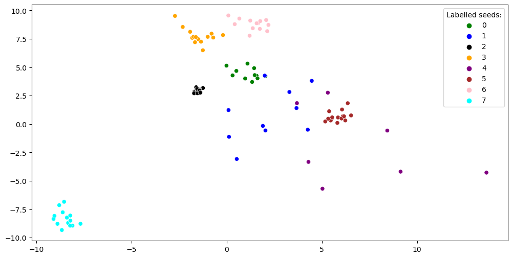
The next example is a two-dimensional data set composed of eight gaussian distributed clusters at different locations and with standard deviations $[0.6,2,0.2,0.7,3,0.4,0.6,0.6]$ (Figure 6). Added to this are many isolated anomalies, and a relatively small anomalous cluster which could also be considered a newly emerging cluster. The total number of points is $10300$, and a small random sample of a $100$ points from the eight clusters are taken as seeds which is illustrated by Figure 7. The number of seeds selected is such that we have at least $10$ per cluster in order to reliably build out the clusters. These would be expected to be provided by a domain expert and help guide the clustering algorithm to desired solutions. Note that the labels can even be a little noisy since mislabelled examples can be ejected out of the group as anomalies during algorithm execution.

Figure 6: Eight gaussian clusters are shown with differing standard deviations ($0.6,2,0.2,0.7,3,0.4,0.6,0.6$) and locations. Added to the data is a scattering of anomalies and also a small anomalous cluster at coordinates $(11,20)$.

Figure 7: A random sample of points (1% of the data) is shown from the gaussian distributed clusters. These form the seeds of the clustering algorithm.

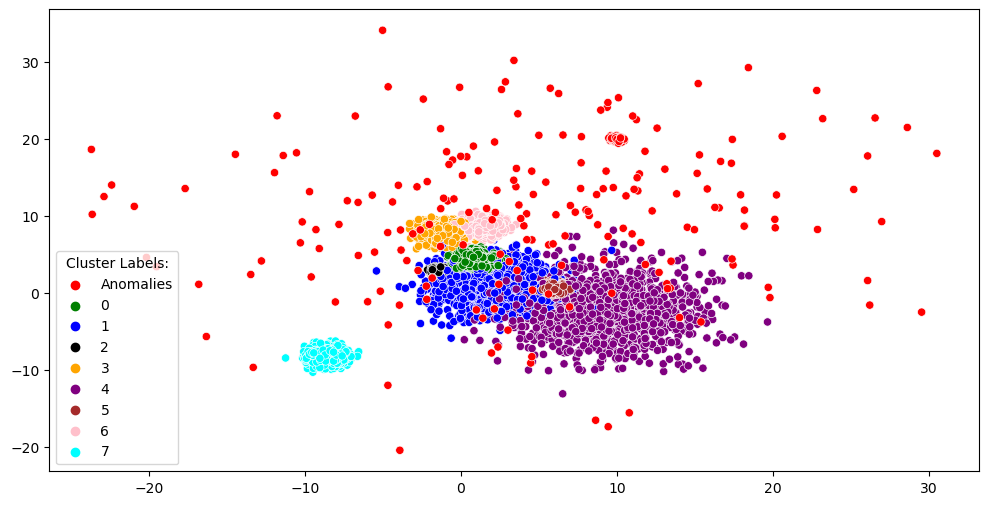
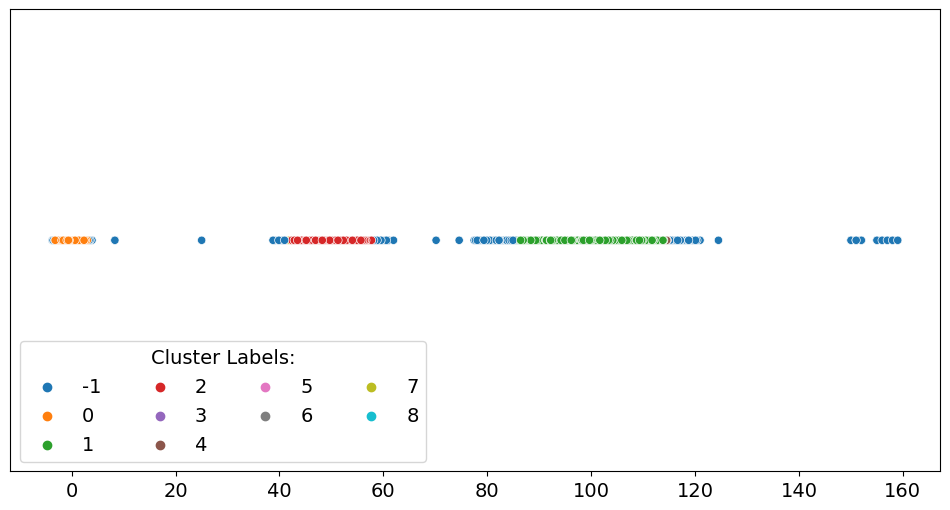
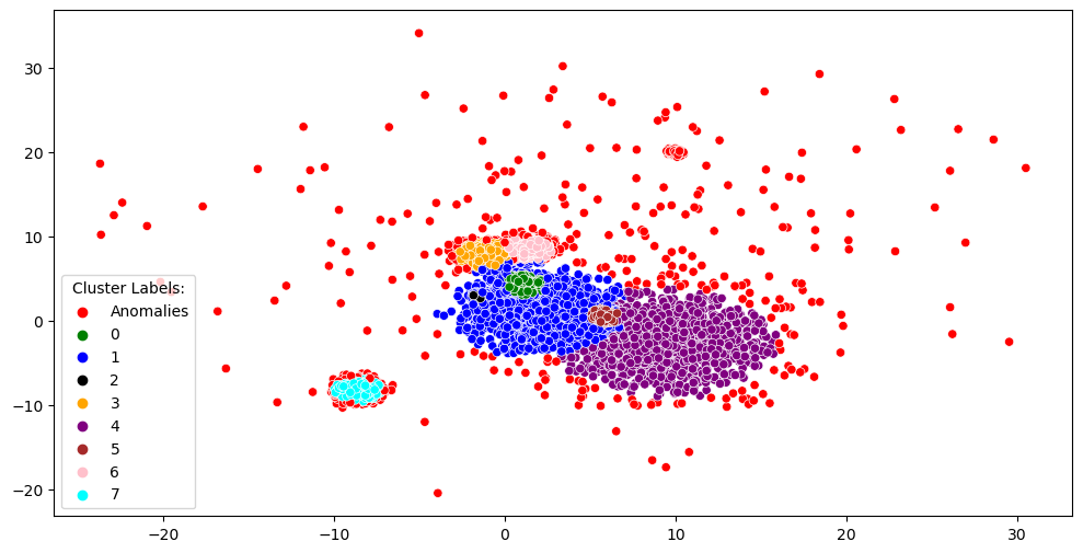
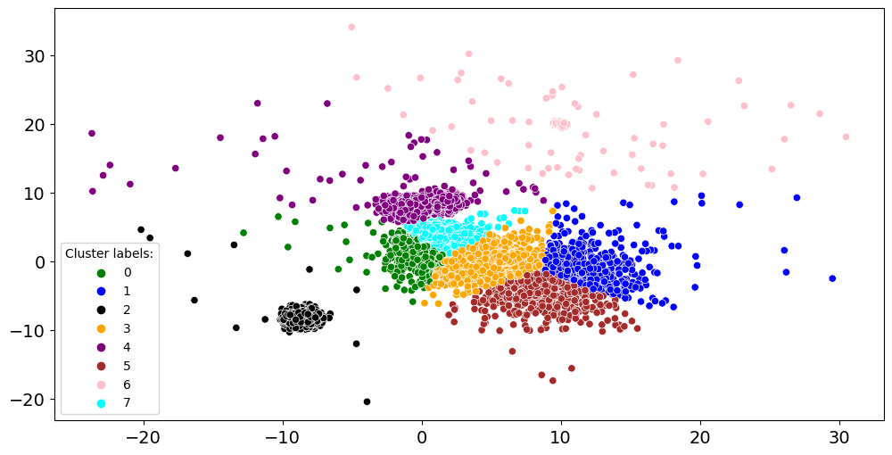
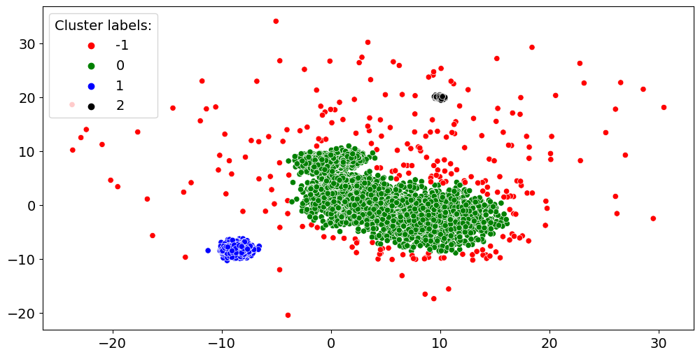
The clustering result is shown in Figure 8 where the eight clusters are largely identified, some points around the clusters are deemed anomalous, and many isolated points and the small cluster labelled as anomalies. Note the difficulty of the task in that some clusters are close or overlapping, while others are located inside another. Hence, there are arguably misclassifications along bordering points. Figure 9 also shows a close up view of one cluster to show the proposed methods ability to highlight fringe and far lying points as outliers with respect to the cluster’s mass of points. Contrasting the results with that of $k$-means ($k=8$), we see in Figure 10 that it unintuitvely partitions the points such that it does not reflect the desired groupings. Clusters originally labelled 3 and 6 are also grouped together and the small anomalous group of points is deemed to be a cluster. $k$-means also partitions all the data points resulting in anomalies being assigned to some cluster. The results obtained with DBSCAN ($mps=15,eps=1.17$) exhibit interesting characteristics. The algorithm successfully identifies and labels many isolated points as outliers, accurately capturing their anomalous nature. It also considers the small group of points to indeed be a cluster. However, it merges the majority of points into one large cluster, leading to a loss of granularity in the clustering results. It also does not report many of the points around the gaussian clusters as anomalies (as in Figure 9). This behavior aligns with the algorithm’s primary objective being to cluster data rather than detect anomalies.

Figure 8: Results of applying the proposed clustering algorithm. The known clusters are largely recovered while points deemed anomalous with respect to the clusters are highlighted.

Figure 9: A close up view of cluster $7$ shows how the proposed clustering algorithm not only detects clusters, but also highlights anomalous points as those being unexpectedly distant from the central mass of points.

Figure 10: Results of $k$-means algorithm ($k=8$). Noteable observations are that some clusters are merged, data is unintuitively partioned and that anomalies are always assigned to some cluster.

Figure 11: Results of the DBSCAN algorithm. Noteable observations are that most of the clusters are reported to be a single large cluster and that many outlying points are highlighted as anomalies.

3.3 Multi-dimensional Realworld Examples

This section presents the clustering algorithm’s results on two widely-used benchmark datasets: MNIST handwritten digits and the 20 newsgroup corpus. These datasets were selected to showcase different application areas and to be easily interpretable for non-experts. Given the high-dimensionality of the raw data in these domains, dimensionality reduction techniques were employed to enhance the clustering outcomes. Specifically, UMAP [7], a method known for its speed and effectiveness with largely default settings was utilised. The distance metric and the desired number of dimensions to map to were the only explicitly specified parameters: the cosine metric was used to address the datasets’ high dimensionality and the number of dimensions set to values that depend on the size of the data.

3.3.1 MNIST Handwritten Digits

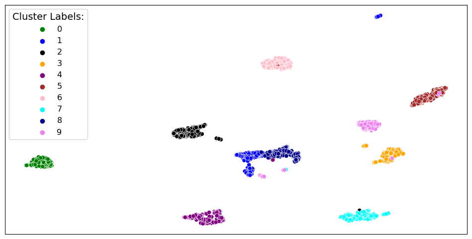
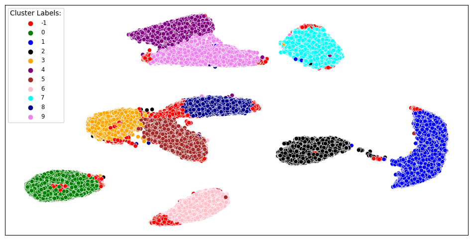
Figure 12 depicts the application of UMAP to 2 dimensions for visualising the smaller MNIST digits dataset, consisting of 1,797 examples available in sklearn [9]. The plot reveals nine prominent clusters along with several smaller groups scattered throughout. The ground truth labels indicate the presence of ten distinct groups, each corresponding to a specific digit. For the clustering algorithm, a mapping to a 10-dimensional space is utilised, and approximately 6% of the data (107 examples) is randomly sampled to provide around 10 labeled items per group, serving as seeds for the algorithm. The clustering results are shown in Figure 13, exhibiting an accuracy of 0.84 according to the ground truth. However, a closer examination of the results unveils an interesting finding: the algorithm not only successfully captures much of the primary clusters but also assigns points that may be outliers with respect to the clusters to the anomalous group. These anomalous parts of clusters or individual small clusters often represent either uniquely written digits, or slight variations within the same class, such as the digit 1 with or without a horizontal baseline.

Figure 12: This illustrates the 2-dimensional UMAP of the smaller MNIST data set obtained from sklearn, using the cosine metric. Each data point is color-coded based on its corresponding class label obtained from the provided labels.

Figure 13: The results of applying the clustering algorithm to the smaller MNIST digits data set obtained from sklearn after performing a UMAP transformation. The actual clustering process involved mapping the data to 10 dimensions. However, for the purpose of visualisation, the results are presented in a 2-dimensional mapping. The accuracy of the clustering according to the ground truth labels is 0.84.

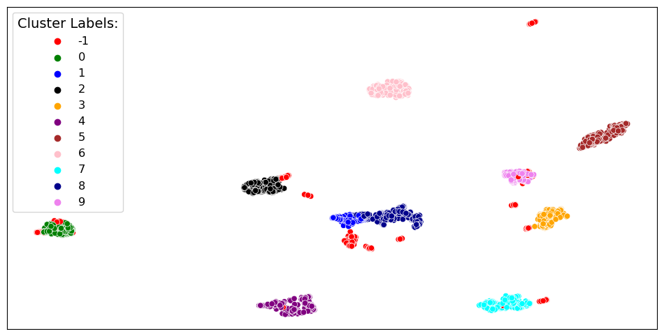
For completeness, Figure 14 shows the algorithm results on the full MNIST digits data set comprising 70,000 examples with UMAP reduction to 20 dimensions due to the much larger data set size. Here an accuracy of 0.92 is achieved according to the ground truth labels by leveraging merely 0.5% (350) of labelled examples as seeds. Notably, despite the substantial expansion in the number of examples, only a modest number of additional samples were required for satisfactory results. Anomalies are also found within different segments of the primary clusters, warranting further investigation to discern whether they signify false positives or alternative representations of a handwritten digit.

Figure 14: The results of applying the clustering algorithm to the full MNIST digits data set after performing a UMAP transformation. The actual clustering process involved mapping the data to 20 dimensions since the data set is much larger. However, for the purpose of visualisation, the results are presented in a 2-dimensional mapping. The accuracy of the clustering according to the ground truth labels is 0.92.

3.3.2 20 Newsgroups Corpus

The 20 Newsgroups data set in the scikit-learn library can be used as an example of clustering data in the text document space. It contains over 18,000 news articles that are organised into 20 categories. In this specific example, a subset of 6 categories is used. These were selected for their distinctness, resulting in a total of 5,881 examples.

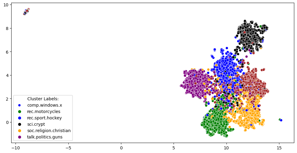
To prepare the data, a standard pre-processing procedure is followed, including lemmatisation, creating a tf-idf matrix, and removing stopwords with a minimum document frequency of five. Due to the high dimensionality of the data, UMAP is employed for dimension reduction, as it effectively preserves the relationships between examples. The resulting reduction to 2 dimensions is illustrated in Figure 15, where each example is coloured according to its ground truth category label. Notably, there is significant overlap between clusters, particularly in the central regions, and a small cluster consisting of examples from all categories can be observed on the far top-left of the plot at approximate coordinates (-8,9).

Figure 15: A 2-dimensional UMAP plot of the 20 Newsgroup data set is shown. Each point is coloured according to its ground truth category.

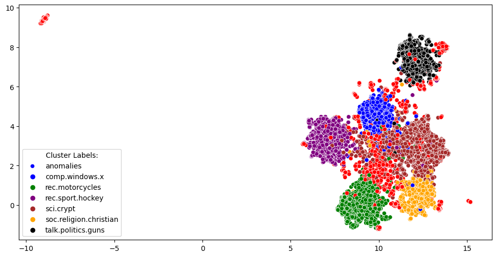
For clustering purposes, the data is mapped to 10 dimensions and a 2% random sample of labelled examples is included to guide the algorithm. This approach incorporates user input to achieve desired outcomes. The clustering results are shown in Figure 16 (displayed over the 2-dimensional mapping). The algorithm successfully recovers most of the six main clusters, achieving an overall accuracy of 0.74 according to the ground truth labels. Moreover, the algorithm flags many examples located between clusters as anomalies, as well as the small dense cluster on the far top-left. This again highlights that the algorithm performs a clustering as opposed to a partitioning of the data points. Table 1 provides the top 10 keywords for each of the six clusters, along with the anomalous group. The keywords align well with the category labels, while the anomalous group consists of seemingly random words that do not align well to any specific category.

Figure 16: The results of applying the proposed semi-supervised clustering algorithm on 6 of the 20 Newsgroup corpus data set categories after a UMAP reduction to 10 dimensions. The accuracy of the clustering according to the ground truth labels is 0.74.

Table 1: Top Cluster Keywords

Category	Keywords
Anomalies	helmet, thanks, edu, just, like, list, mail, com, dog, wa
comp.windows.x	use, display, application, program, motif, widget, thanks, file, server, window
rec.motorcycles	rider, road, just, like, riding, dod, motorcycle, ride, wa, bike
rec.sport.hockey	espn, season, playoff, play, year, player, hockey, wa, team, game
sci.crypt	escrow, use, nsa, algorithm, phone, government, encryption, clipper, chip, key
soc.religion.christian	christians, bible, people, sin, christ, christian, church, jesus, wa, god
talk.politics.guns	just, weapon, government, law, did, right, fbi, people, wa, gun

4 Conclusion

The present work introduces two significant contributions. Firstly, inspired by David Marr’s tri-level hypothesis for information processing, it presents a computable definition of a cluster. This definition is derived by analysing elements of human visual clustering and assuming certain constraints deemed true of the real world. A key observation is that a cluster is a collection of points devoid of any anomalies with respect to a given grouping principle and measure. This sheds light on the dual nature of clustering and anomaly detection, highlighting their interdependence and the role of data representations and measures in achieving desired groupings.

Secondly, a novel semi-supervised clustering algorithm is proposed whose kernel is based on the anomaly detection work by Mohammad [8]. This work gave a precise computable definition of what constitutes an anomaly and provides a compelling rationale for accepting such a definition. Additionally, an efficient algorithm to compute anomalies based on the Euclidean distance from the median is provided. The clustering algorithm operates on numerical data and utilises a small amount of labelled examples for initialisation, guidance, and subsequent expansion of clusters. The algorithm handles noisy labelled data by ejecting distinctly incorrect points from the groups. Instead of aiming for a complete partitioning of all the data, the algorithm focuses on clustering the data, thus ensuring that anomalies and unknown clusters are not forcibly assigned to existing clusters. Such instances are left to be analysed in subsequent steps.

The results of the semi-supervised clustering algorithm are compared with those of popular unsupervised clustering algorithms, namely $k$-means and DBSCAN. The synthetic data examples showcased the algorithm’s ability to build clusters even with a relatively small number of examples per cluster and accommodated clusters of different densities. In contrast, $k$-means and DBSCAN exhibited undesired results in these examples due to their inherent constraints and assumptions. In particular $k$-means gave unintuitive partitions that split clusters or assigned clearly anomalous points to a cluster. On the other hand, DBSCAN proved to be sensitive to the supplied parameters where clusters either got merged or split because of its inability to locally adapt.

The incorporation of dimension reduction techniques, particularly UMAP, in conjunction with semi-supervised clustering, has proven to be highly advantageous. This is exemplified through the analysis of image and text data examples. The employed workflow, which encompasses dimension reduction for visualisation, sample labelling, and clustering, offers significant benefits in the identification of clusters. Notably, it recognises the importance of not forcibly assigning every example, including anomalies and points from unknown clusters, to specific clusters. Instead, the approach allows for a more nuanced treatment of data points, facilitating the identification of clusters while acknowledging the presence of ungrouped instances. These examples also showed that user interaction and sampling remain important even after UMAP visualisation, as points appearing visually close together may not belong to the same group. An example illustrating this phenomenon can be found in the MNIST digits mapping (Figure 13), where the clusters of digits 8’s and 1’s exhibit visual proximity while representing separate clusters.

Clustering is an interactive and iterative process that combines exploration and analysis. Merely applying an algorithm without understanding the data and the problem space is not recommended, and results are never accepted blindly. During the exploratory phase, it is important to gain familiarity with the data and establish certain assumptions that constrain solutions, such as the type and number of clusters, the possibility of clusters forming hyper-spherical groupings, algorithm parameters, or the labelling of points for seeding and guiding an algorithm. In the presented semi-supervised clustering algorithm, the explicit constraints are taken to be labelled examples as opposed to parameter specification, and implicit is the choice of grouping law and measure. However, note the difference between knowledge of a few labelled examples per cluster and estimating parameters such as the $k$ in $k$-means or $mps$ and $eps$ in DBSCAN. In the former case clusters can be gradually built over the labelled subset, and then expanded upon, without requiring knowledge of samples from all the clusters. Furthermore, being parameter-free relieves users of one of the main challenges commonly encountered in unsupervised learning problems.

The presented work highlights how all algorithms constrain solutions, thereby reducing the number of possible groupings that can be returned. However, it is postulated that only relatively few grouping principles are of actual interest. These principles and appropriate measures constrain what groupings are acceptable a-prori, particularly when formulated through representation and unexpectedness. Hence, a realist position is adopted, where clustering is deemed an objective process as opposed to a purely subjective experience.

In future research, the exploration of additional grouping principles and measures, extending beyond proximity and the Euclidean distance to the median, will be undertaken. This expansion aims to enhance the versatility and effectiveness of the clustering algorithm. Moreover, the inherent speed and nature of the algorithm also makes it well-suited for online clustering scenarios. Consequently, an extension of the algorithm to handle the assignment of new points to existing clusters and the identification of anomalies that may potentially form new clusters will be investigated.

References

- Basu et al. [2004] Sugato Basu, Arindam Banerjee, and Raymond J. Mooney. Active semi-supervision for pairwise constrained clustering. Proceedings of the tenth ACM SIGKDD international conference on Knowledge discovery and data mining, pages 333–342, 2004.
- Desolneux et al. [2007] Agns Desolneux, Lionel Moisan, and Jean-Michel Morel. From Gestalt Theory to Image Analysis: A Probabilistic Approach. Springer Publishing Company, Incorporated, 1st edition, 2007. ISBN 0387726357.
- Ester et al. [1996] Martin Ester, Hans-Peter Kriegel, Jörg Sander, and Xiaowei Xu. A density-based algorithm for discovering clusters in large spatial databases with noise. Proceedings of the 2nd International Conference on Knowledge Discovery and Data Mining (KDD), pages 226–231, 1996.
- Forgy [1965] E. Forgy. Cluster analysis of multivariate data: Efficiency versus interpretability of classification. Biometrics, 21(3):768–769, 1965.
- MacQueen [1967] J. MacQueen. Some methods for classification and analysis of multivariate observations. In Proceedings of the Fifth Berkeley Symposium on Mathematical Statistics and Probability, Volume 1: Statistics, pages 281–297, Berkeley, Calif., 1967. University of California Press.
- Marr [1982] David Marr. Vision: A Computational Investigation into the Human Representation and Processing of Visual Information. Henry Holt and Co., Inc., USA, 1982. ISBN 0716715678.
- McInnes et al. [2018] Leland McInnes, John Healy, and James Melville. Umap: Uniform manifold approximation and projection for dimension reduction. arXiv preprint arXiv:1802.03426, 2018.
- Mohammad [2021] Nassir Mohammad. Anomaly detection using principles of human perception, 2021.
- Pedregosa et al. [2011] F. Pedregosa, G. Varoquaux, A. Gramfort, V. Michel, B. Thirion, O. Grisel, M. Blondel, P. Prettenhofer, R. Weiss, V. Dubourg, J. Vanderplas, A. Passos, D. Cournapeau, M. Brucher, M. Perrot, and E. Duchesnay. Scikit-learn: Machine learning in Python. Journal of Machine Learning Research, 12:2825–2830, 2011.
- Wagstaff et al. [2001] Kiri Wagstaff, Claire Cardie, Seth Rogers, and Stefan Schrödl. Constrained k-means clustering with background knowledge. In ICML, pages 577–584, 2001.
- Ward Jr [1963] Joe H Ward Jr. Hierarchical grouping to optimize an objective function. Journal of the American Statistical Association, 58(301):236–244, 1963.