\makesavenoteenv

longtable \KOMAoptioncaptionstableheading

Revisiting Whittaker-Henderson Smoothing

Guillaume Biessy111guillaume.biessy78@gmail.com    PhD    LinkPact222LinkPact, 80 boulevard Pasteur, 75015 Paris, France and Sorbonne Université333Sorbonne Université, CNRS, Laboratoire de Probabilités, Statistique et Modélisation, LPSM, 4 place Jussieu, 75005 Paris, France
(September 16, 2023)
Abstract

Introduced nearly a century ago, Whittaker-Henderson smoothing remains one of the most commonly used methods by actuaries for constructing one-dimensional and two-dimensional experience tables for mortality and other Life Insurance risks. This paper proposes to reframe this smoothing technique within a modern statistical framework and addresses six questions of practical interest regarding its use.

Firstly, we adopt a Bayesian view of this smoothing method to build credible intervals. Next, we shed light on the choice of observation vectors and weights to which the smoothing should be applied by linking it to a maximum likelihood estimator introduced in the context of duration models. We then enhance the precision of the smoothing by relaxing an implicit asymptotic approximation on which it relies. Afterward, we select the smoothing parameters based on maximizing a marginal likelihood. We later improve numerical performance in the presence of a large number of observation points and, consequently, parameters. Finally, we extrapolate the results of the smoothing while preserving consistency between estimated and predicted values through the use of constraints.

Keywords: smoothing methods, duration models, experience tables, maximum likelihood, generalized additive models, empirical Bayesian approach, marginal likelihood, extrapolation.

1 Introduction

1.1 Notations

In this paper, vector names are written in bold characters and matrix names in uppercase letters. If 𝐲𝐲\mathbf{y} is a vector and A𝐴A is a matrix, Var(𝐲)Var𝐲\text{Var}(\mathbf{y}) denotes the variance-covariance matrix associated with 𝐲𝐲\mathbf{y}, diag(A)diag𝐴\textbf{diag}(A) represents the diagonal of matrix A𝐴A, and Diag(𝐲)Diag𝐲\text{Diag}(\mathbf{y}) is the diagonal matrix such that diag(Diag(𝐲))=𝐲diagDiag𝐲𝐲\textbf{diag}(\text{Diag}(\mathbf{y}))=\mathbf{y}. The sum of the diagonal elements of A𝐴A is denoted as tr(A)tr𝐴\text{tr}(A) and its transpose as ATsuperscript𝐴𝑇A^{T}. In the case where A𝐴A is invertible, A1superscript𝐴1A^{-1} denotes its inverse, ATsuperscript𝐴𝑇A^{-T} is the inverse of its transpose, and |A|𝐴|A| is the product of the eigenvalues of A𝐴A. For a non-invertible matrix A𝐴A, Asuperscript𝐴A^{-} refers to the Moore-Penrose pseudoinverse of A𝐴A, and |A|+subscript𝐴|A|_{+} denotes the product of the non-zero eigenvalues of A𝐴A. By writing the eigendecomposition as A=UΣVT𝐴𝑈Σsuperscript𝑉𝑇A=U\Sigma V^{T}, where U𝑈U and V𝑉V are two orthogonal matrices and ΣΣ\Sigma is a diagonal matrix containing the eigenvalues of A𝐴A, and by denoting ΣsuperscriptΣ\Sigma^{-} as the matrix obtained by replacing the non-zero eigenvalues in ΣΣ\Sigma with their inverses while keeping the zero eigenvalues unchanged, the pseudoinverse is given by A=VΣUTsuperscript𝐴𝑉superscriptΣsuperscript𝑈𝑇A^{-}=V\Sigma^{-}U^{T}. The Kronecker product of two matrices A𝐴A and B𝐵B is denoted as ABtensor-product𝐴𝐵A\otimes B, and their Hadamard product, or element-wise product, is denoted as ABdirect-product𝐴𝐵A\odot B. vec(A)vec𝐴\textbf{vec}(A) represents the vector obtained by stacking the columns of matrix A𝐴A together. Finally, the symbol proportional-to\propto signifies a proportional relationship between the expressions on both sides of it.

1.2 Origin

Whittaker-Henderson smoothing is a gradation method aimed at correcting the effect of sampling fluctuations on an observation vector. It is applied to evenly-spaced discrete observations. Initially proposed by Whittaker (1922) for constructing mortality tables and further developed by the works of Henderson (1924), it remains one of the most popular methods among actuaries for constructing experience tables in life insurance. Extending to two-dimensional tables, it can be used for studying various risks, including but not limited to mortality, disability, long-term care, lapse, mortgage default, and unemployment.

1.3 The one-dimensional case

Let 𝐲𝐲\mathbf{y} be a vector of observations and 𝐰𝐰\mathbf{w} a vector of positive weights, both of size n𝑛n. The estimator associated with Whittaker-Henderson smoothing is given by:

𝐲^=argmin𝜽{F(𝐲,𝐰,𝜽)+Rλ,q(𝜽)}^𝐲𝜽argmin𝐹𝐲𝐰𝜽subscript𝑅𝜆𝑞𝜽\hypertarget{eq-WH1}{}{\hat{\mathbf{y}}=\underset{\boldsymbol{\theta}}{\text{argmin}}\{F(\mathbf{y},\mathbf{w},\boldsymbol{\theta})+R_{\lambda,q}(\boldsymbol{\theta})\}} (1)

where:

  • \bullet

    F(𝐲,𝐰,𝜽)=i=1𝑛wi(yiθi)2𝐹𝐲𝐰𝜽𝑖1𝑛subscript𝑤𝑖superscriptsubscript𝑦𝑖subscript𝜃𝑖2F(\mathbf{y},\mathbf{w},\boldsymbol{\theta})=\underset{i=1}{\overset{n}{\sum}}w_{i}(y_{i}-\theta_{i})^{2} represents a fidelity criterion to the observations,

  • \bullet

    Rλ,q(𝜽)=λi=1nq(Δq𝜽)i2subscript𝑅𝜆𝑞𝜽𝜆𝑖1𝑛𝑞superscriptsubscriptsuperscriptΔ𝑞𝜽𝑖2R_{\lambda,q}(\boldsymbol{\theta})=\lambda\underset{i=1}{\overset{n-q}{\sum}}(\Delta^{q}\boldsymbol{\theta})_{i}^{2} represents a smoothness criterion.

In the latter expression, ΔqsuperscriptΔ𝑞\Delta^{q} denotes the forward difference operator of order q𝑞q, such that for any i[1,nq]𝑖1𝑛𝑞i\in[1,n-q]:

(Δq𝜽)i=k=0𝑞(qk)(1)qkθi+k.subscriptsuperscriptΔ𝑞𝜽𝑖𝑘0𝑞matrix𝑞𝑘superscript1𝑞𝑘subscript𝜃𝑖𝑘(\Delta^{q}\boldsymbol{\theta})_{i}=\underset{k=0}{\overset{q}{\sum}}\begin{pmatrix}q\\ k\end{pmatrix}(-1)^{q-k}\theta_{i+k}.

Let us define W=Diag(𝐰)𝑊Diag𝐰W=\text{Diag}(\mathbf{w}), the diagonal matrix of weights, and Dn,qsubscript𝐷𝑛𝑞D_{n,q} as the order q𝑞q difference matrix of dimensions (nq)×n𝑛𝑞𝑛(n-q)\times n, such that (Dn,q𝜽)i=(Δq𝜽)isubscriptsubscript𝐷𝑛𝑞𝜽𝑖subscriptsuperscriptΔ𝑞𝜽𝑖(D_{n,q}\boldsymbol{\theta})_{i}=(\Delta^{q}\boldsymbol{\theta})_{i} for all i[1,nq]𝑖1𝑛𝑞i\in[1,n-q]. The most commonly used difference matrices of order 1 and 2 have the following forms:

Dn,1=[110001100011]andDn,2=[121000121000121].formulae-sequencesubscript𝐷𝑛1matrix110001100011andsubscript𝐷𝑛2matrix121000121000121D_{n,1}=\begin{bmatrix}-1&1&0&\ldots&0\\ 0&-1&1&\ldots&0\\ \vdots&\vdots&\vdots&\ddots&\vdots\\ 0&\ldots&0&-1&1\\ \end{bmatrix}\quad\text{and}\quad D_{n,2}=\begin{bmatrix}1&-2&1&0&\ldots&0\\ 0&1&-2&1&\ldots&0\\ \vdots&\vdots&\vdots&\vdots&\ddots&\vdots\\ 0&\ldots&0&1&-2&1\\ \end{bmatrix}.

The fidelity and smoothness criteria can be rewritten in matrix form as:

F(𝐲,𝐰,𝜽)=(𝐲𝜽)TW(𝐲𝜽)andRλ,q(𝜽)=λ𝜽TDn,qTDn,q𝜽.formulae-sequence𝐹𝐲𝐰𝜽superscript𝐲𝜽𝑇𝑊𝐲𝜽andsubscript𝑅𝜆𝑞𝜽𝜆superscript𝜽𝑇superscriptsubscript𝐷𝑛𝑞𝑇subscript𝐷𝑛𝑞𝜽F(\mathbf{y},\mathbf{w},\boldsymbol{\theta})=(\mathbf{y}-\boldsymbol{\theta})^{T}W(\mathbf{y}-\boldsymbol{\theta})\quad\text{and}\quad R_{\lambda,q}(\boldsymbol{\theta})=\lambda\boldsymbol{\theta}^{T}D_{n,q}^{T}D_{n,q}\boldsymbol{\theta}.

The associated estimator for smoothing becomes:

𝐲^=argmin𝜽{(𝐲𝜽)TW(𝐲𝜽)+𝜽TPλ𝜽}^𝐲𝜽argminsuperscript𝐲𝜽𝑇𝑊𝐲𝜽superscript𝜽𝑇subscript𝑃𝜆𝜽\hypertarget{eq-WH2}{}{\hat{\mathbf{y}}=\underset{\boldsymbol{\theta}}{\text{argmin}}\left\{(\mathbf{y}-\boldsymbol{\theta})^{T}W(\mathbf{y}-\boldsymbol{\theta})+\boldsymbol{\theta}^{T}P_{\lambda}\boldsymbol{\theta}\right\}} (2)

where Pλ=λDn,qTDn,qsubscript𝑃𝜆𝜆superscriptsubscript𝐷𝑛𝑞𝑇subscript𝐷𝑛𝑞P_{\lambda}=\lambda D_{n,q}^{T}D_{n,q}.

1.4 The two-dimensional case

In the two-dimensional case, let us consider a matrix Y𝑌Y of observations and a matrix ΩΩ\Omega of non-negative weights, both of dimensions nx×nzsubscript𝑛𝑥subscript𝑛𝑧n_{x}\times n_{z}. The estimator associated with the Whittaker-Henderson smoothing can be written as:

Y^=argminΘ{F(Y,Ω,Θ)+Rλ,q(Θ)}^𝑌Θargmin𝐹𝑌ΩΘsubscript𝑅𝜆𝑞Θ\widehat{Y}=\underset{\Theta}{\text{argmin}}\{F(Y,\Omega,\Theta)+R_{\lambda,q}(\Theta)\}

where:

  • \bullet

    F(Y,Ω,Θ)=i=1nxj=1nzΩi,j(Yi,jΘi,j)2𝐹𝑌ΩΘsuperscriptsubscript𝑖1subscript𝑛𝑥superscriptsubscript𝑗1subscript𝑛𝑧subscriptΩ𝑖𝑗superscriptsubscript𝑌𝑖𝑗subscriptΘ𝑖𝑗2F(Y,\Omega,\Theta)=\sum_{i=1}^{n_{x}}\sum_{j=1}^{n_{z}}\Omega_{i,j}(Y_{i,j}-\Theta_{i,j})^{2} represents a fidelity criterion to the observations,

  • \bullet

    Rλ,q(Θ)=λxj=1nzi=1nxqx(ΔqxΘ,j)i2+λzi=1nxj=1nzqz(ΔqzΘi,)j2subscript𝑅𝜆𝑞Θsubscript𝜆𝑥superscriptsubscript𝑗1subscript𝑛𝑧superscriptsubscript𝑖1subscript𝑛𝑥subscript𝑞𝑥superscriptsubscriptsuperscriptΔsubscript𝑞𝑥subscriptΘ𝑗𝑖2subscript𝜆𝑧superscriptsubscript𝑖1subscript𝑛𝑥superscriptsubscript𝑗1subscript𝑛𝑧subscript𝑞𝑧superscriptsubscriptsuperscriptΔsubscript𝑞𝑧subscriptΘ𝑖𝑗2R_{\lambda,q}(\Theta)=\lambda_{x}\sum_{j=1}^{n_{z}}\sum_{i=1}^{n_{x}-q_{x}}(\Delta^{q_{x}}\Theta_{\bullet,j})_{i}^{2}+\lambda_{z}\sum_{i=1}^{n_{x}}\sum_{j=1}^{n_{z}-q_{z}}(\Delta^{q_{z}}\Theta_{i,\bullet})_{j}^{2} is a smoothness criterion.

This latter criterion can be written as the sum of two one-dimensional regularization criteria, with orders qxsubscript𝑞𝑥q_{x} and qzsubscript𝑞𝑧q_{z}, applied respectively to all rows and all columns of ΘΘ\Theta. It is also possible to adopt matrix notations by defining 𝐲=vec(Y)𝐲vec𝑌\mathbf{y}=\textbf{vec}(Y), 𝐰=vec(Ω)𝐰vecΩ\mathbf{w}=\textbf{vec}(\Omega), and 𝜽=vec(Θ)𝜽vecΘ\boldsymbol{\theta}=\textbf{vec}(\Theta) as the vectors obtained by stacking the columns of the matrices Y𝑌Y, ΩΩ\Omega, and ΘΘ\Theta, respectively. Additionally, let us denote W=Diag(𝐰)𝑊Diag𝐰W=\text{Diag}(\mathbf{w}) and n=nx×nz𝑛subscript𝑛𝑥subscript𝑛𝑧n=n_{x}\times n_{z}. The fidelity and smoothness criteria can then be rewritten as linear combinations of the vectors 𝐲𝐲\mathbf{y}, 𝐰𝐰\mathbf{w}, and 𝜽𝜽\boldsymbol{\theta}:

F(𝐲,𝐰,𝜽)𝐹𝐲𝐰𝜽\displaystyle F(\mathbf{y},\mathbf{w},\boldsymbol{\theta}) =(𝐲𝜽)TW(𝐲𝜽)absentsuperscript𝐲𝜽𝑇𝑊𝐲𝜽\displaystyle=(\mathbf{y}-\boldsymbol{\theta})^{T}W(\mathbf{y}-\boldsymbol{\theta})
Rλ,q(𝜽)subscript𝑅𝜆𝑞𝜽\displaystyle R_{\lambda,q}(\boldsymbol{\theta}) =𝜽T(λxInzDnx,qxTDnx,qx+λzDnz,qzTDnz,qzInx)𝜽.absentsuperscript𝜽𝑇tensor-productsubscript𝜆𝑥subscript𝐼subscript𝑛𝑧superscriptsubscript𝐷subscript𝑛𝑥subscript𝑞𝑥𝑇subscript𝐷subscript𝑛𝑥subscript𝑞𝑥tensor-productsubscript𝜆𝑧superscriptsubscript𝐷subscript𝑛𝑧subscript𝑞𝑧𝑇subscript𝐷subscript𝑛𝑧subscript𝑞𝑧subscript𝐼subscript𝑛𝑥𝜽\displaystyle=\boldsymbol{\theta}^{T}(\lambda_{x}I_{n_{z}}\otimes D_{n_{x},q_{x}}^{T}D_{n_{x},q_{x}}+\lambda_{z}D_{n_{z},q_{z}}^{T}D_{n_{z},q_{z}}\otimes I_{n_{x}})\boldsymbol{\theta}.

and the estimator associated with the smoothing takes the form:

𝐲^=argmin𝜽{(𝐲𝜽)TW(𝐲𝜽)+𝜽TPλ𝜽}^𝐲𝜽argminsuperscript𝐲𝜽𝑇𝑊𝐲𝜽superscript𝜽𝑇subscript𝑃𝜆𝜽\hat{\mathbf{y}}=\underset{\boldsymbol{\theta}}{\text{argmin}}\left\{(\mathbf{y}-\boldsymbol{\theta})^{T}W(\mathbf{y}-\boldsymbol{\theta})+\boldsymbol{\theta}^{T}P_{\lambda}\boldsymbol{\theta}\right\}

of Equation 2 except in this case Pλ=λxInzDnx,qxTDnx,qx+λzDnz,qzTDnz,qzInxsubscript𝑃𝜆tensor-productsubscript𝜆𝑥subscript𝐼subscript𝑛𝑧superscriptsubscript𝐷subscript𝑛𝑥subscript𝑞𝑥𝑇subscript𝐷subscript𝑛𝑥subscript𝑞𝑥tensor-productsubscript𝜆𝑧superscriptsubscript𝐷subscript𝑛𝑧subscript𝑞𝑧𝑇subscript𝐷subscript𝑛𝑧subscript𝑞𝑧subscript𝐼subscript𝑛𝑥P_{\lambda}=\lambda_{x}I_{n_{z}}\otimes D_{n_{x},q_{x}}^{T}D_{n_{x},q_{x}}+\lambda_{z}D_{n_{z},q_{z}}^{T}D_{n_{z},q_{z}}\otimes I_{n_{x}}.

1.5 Explicit solution

Equation 2 has an explicit solution:

𝐲^=(W+Pλ)1W𝐲.^𝐲superscript𝑊subscript𝑃𝜆1𝑊𝐲\hypertarget{eq-WH3}{}{\hat{\mathbf{y}}=(W+P_{\lambda})^{-1}W\mathbf{y}.} (3)

Indeed, as a minimum, 𝐲^^𝐲\hat{\mathbf{y}} satisfies:

0=𝜽|𝐲^{(𝐲𝜽)TW(𝐲𝜽)+𝜽TPλ𝜽}=2XTW(y𝐲^)+2XTPλ𝐲^.0evaluated-at𝜽^𝐲superscript𝐲𝜽𝑇𝑊𝐲𝜽superscript𝜽𝑇subscript𝑃𝜆𝜽2superscript𝑋𝑇𝑊𝑦^𝐲2superscript𝑋𝑇subscript𝑃𝜆^𝐲0=\left.\frac{\partial}{\partial\boldsymbol{\theta}}\right|_{\hat{\mathbf{y}}}\left\{(\mathbf{y}-\boldsymbol{\theta})^{T}W(\mathbf{y}-\boldsymbol{\theta})+\boldsymbol{\theta}^{T}P_{\lambda}\boldsymbol{\theta}\right\}=-2X^{T}W(y-\hat{\mathbf{y}})+2X^{T}P_{\lambda}\hat{\mathbf{y}}.

It follows that (W+Pλ)𝐲^=W𝐲𝑊subscript𝑃𝜆^𝐲𝑊𝐲(W+P_{\lambda})\hat{\mathbf{y}}=W\mathbf{y}, and if W+Pλ𝑊subscript𝑃𝜆W+P_{\lambda} is invertible, then 𝐲^^𝐲\hat{\mathbf{y}} is indeed a solution of Equation 3. When λ0𝜆0\lambda\neq 0, W+Pλ𝑊subscript𝑃𝜆W+P_{\lambda} is invertible as long as 𝐰𝐰\mathbf{w} has q𝑞q non-zero elements in the one-dimensional case, and ΩΩ\Omega has at least qx×qzsubscript𝑞𝑥subscript𝑞𝑧q_{x}\times q_{z} non-zero elements distributed over qxsubscript𝑞𝑥q_{x} different rows and qzsubscript𝑞𝑧q_{z} different columns in the two-dimensional case. These sufficient conditions are always satisfied in practice and will not be demonstrated here.

1.6 Impact of the smoothing parameter(s)

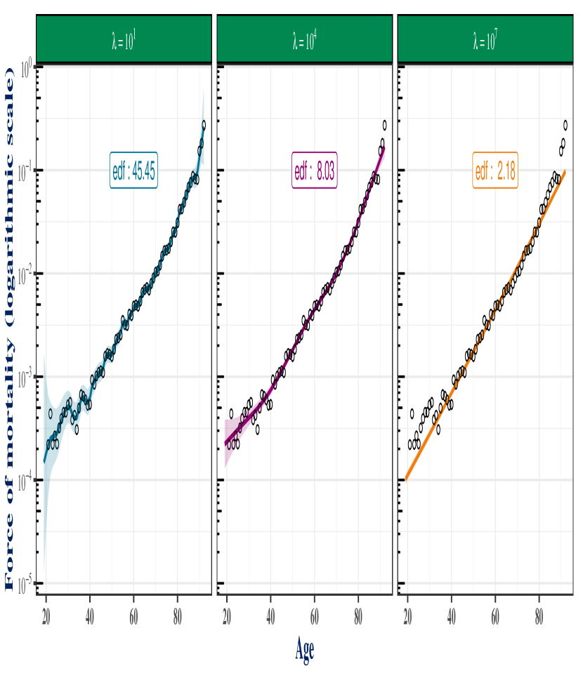
In Equation 1 (𝐲𝜽)TW(𝐲𝜽)superscript𝐲𝜽𝑇𝑊𝐲𝜽(\mathbf{y}-\boldsymbol{\theta})^{T}W(\mathbf{y}-\boldsymbol{\theta}) represents a fidelity criterion to the observations and 𝜽TPλ𝜽superscript𝜽𝑇subscript𝑃𝜆𝜽\boldsymbol{\theta}^{T}P_{\lambda}\boldsymbol{\theta} represents a smoothness criterion. The relative importance of these criteria is controlled by the parameter (or pair of parameters in the two-dimensional case) λ𝜆\lambda. Figure 1 provides an illustration of one-dimensional smoothing on mortality data using three different values of the smoothing parameter. The effective degrees of freedom shown in this figure can be calculated by summing the diagonal values of H𝐻H, the hat matrix of the model. The hat matrix satisfies 𝐲^=H𝐲^𝐲𝐻𝐲\hat{\mathbf{y}}=H\mathbf{y} and can be identified in Equation 3 as H=(W+Pλ)1W𝐻superscript𝑊subscript𝑃𝜆1𝑊H=(W+P_{\lambda})^{-1}W. These effective degrees of freedom serve as a non-parametric equivalent of the number of independent parameters in parametric models but can take non-integer values. The concept of degrees of freedom will be discussed in more detail in Section 6 of the paper. It can be observed here that the result of smoothing is highly sensitive to the chosen value of the smoothing parameter. The choice of λ=101𝜆superscript101\lambda=10^{1} leads to a highly volatile fit that largely reproduces the sampling fluctuations present in the data. On the other hand, the choice of λ=107𝜆superscript107\lambda=10^{7} seems too rigid to capture the underlying pattern of the data. The choice of λ=104𝜆superscript104\lambda=10^{4} appears, at first glance, as a satisfactory compromise between these two extremes.
Refer to caption
Figure 1: Whittaker-Henderson smoothing applied to a portfolio of synthetic mortality data for 3 choices of the smoothing parameter. The points represent the initial observations, the curves depict the result of the smoothing, and the shaded areas represent the associated credibility intervals. edf refers to the effective degrees of freedom of the model.

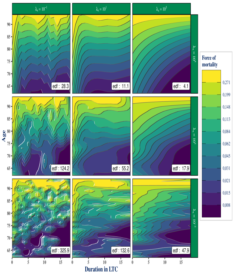
In the two-dimensional case, two penalties are applied to the model parameters. Figure 2 illustrates the application of smoothing to mortality data for a portfolio of insured individuals with dependence, based on the age of the insured individuals and their duration in the dependent state. Different combinations of the two smoothing parameters in this model are used to produce the 9 smoothers represented in this figure. While some combinations of smoothing parameters may be deemed implausible, such as those associated with the choice λx=100subscript𝜆𝑥superscript100\lambda_{x}=10^{0}, it is challenging in the two-dimensional case to determine graphically which combination of parameters is most suitable. The selection of the smoothing parameter will be discussed in detail in Section 5.
Refer to caption
Figure 2: Whittaker-Henderson smoothing applied to a synthetic portfolio of policyholders in long-term care situation for 9 combinations of smoothing parameters. The contour lines and colors depict the surface of the smoothed mortality force as a function of the age of the policyholders and the duration in the long-term care state.

1.7 Plan for the paper

This paper aims to address 6 practical questions associated with the use of Whittaker-Henderson smoothing, each of which will be covered in a dedicated section.

1.7.1 How to measure uncertainty in smoothing results?

We propose to measure the uncertainty in smoothing results based on the available observation volume. In a frequentist approach, the estimator associated with smoothing appears to be biased, which makes it challenging to construct relevant confidence intervals for it. However, smoothing can be naturally interpreted in a Bayesian framework, allowing the construction of credible intervals.

1.7.2 Which observation and weight vectors to use?

Candidates are proposed for the vectors 𝐲𝐲\mathbf{y} and 𝐰𝐰\mathbf{w}. By adopting the framework of duration models used for experience rating and considering the maximum likelihood estimator of crude rates under the assumption of piecewise constant transition intensity, we present a couple (𝐲,𝐰)𝐲𝐰(\mathbf{y},\mathbf{w}) that satisfies the implicit conditions associated with the use of smoothing in an asymptotic sense.

1.7.3 How to improve the accuracy of smoothing with limited data volume?

The previous theoretical framework is based on an asymptotic approximation, which, in many practical situations where the available data volume is limited, can be biased. We propose a generalization of Whittaker-Henderson smoothing based on exact likelihood rather than its normal approximation. This approach requires iterative solving of penalized likelihood equations. By comparing this exact approach with the normal approximation associated with the initial smoothing, we show that this approximation can sometimes come at the cost of substantial bias in the obtained results.

1.7.4 How to choose the smoothing parameter(s)?

We then address the choice of the smoothing parameter λ𝜆\lambda to use. This parameter controls the strength of the applied smoothing and has a crucial impact on the obtained results. To select this parameter, we propose maximizing a marginal likelihood using the optimization methods of Brent (1973) and John A. Nelder and Mead (1965), employed in the one-dimensional and two-dimensional case, respectively. These methods are implemented through the optimize and optim functions in the stats library of the statistical programming language R. In the context of the proposed generalization of smoothing, where solving likelihood equations and selecting the smoothing parameter are performed through nested iterations, we compare the precision and computational time of two known strategies called outer iteration and performance iteration. These strategies differ in the order in which the iterations are nested, and we demonstrate that the latter approach significantly reduces computation time at the cost of negligible loss of precision.

1.7.5 How to improve smoothing performance with a large number of data points?

We propose a practical solution to accelerate smoothing when the number of observations - and thus parameters - is substantial. This situation is common in practice, especially for two-dimensional tables used in the modeling of disability and long-term care risks. To address this issue, an eigendecomposition of the one-dimensional penalization matrices involved in smoothing is used. This decomposition provides a new interpretation of smoothing and opens the door to the use of a rank reduction method to reduce the number of parameters used and the computational time, while incurring minimal loss of precision.

1.7.6 How to extrapolate smoothing results?

Finally, we cover the problem of extrapolation in smoothing, which involves solving a modified version of the initial optimization problem where the fidelity criterion remains unchanged and the smoothness criterion is extended to extrapolated values. In the one-dimensional case, a solution may immediately be obtained. However, in the two-dimensional case, as shown by Carballo, Durban, and Lee (2021), constraints must be imposed on the model to prevent the extrapolation step from altering the results obtained during the initial use of the smoothing.

2 How to measure uncertainty in smoothing results?

Equation 3 indicates that 𝔼(𝐲^)=(W+Pλ)1W𝔼(𝐲)𝔼(𝐲)𝔼^𝐲superscript𝑊subscript𝑃𝜆1𝑊𝔼𝐲𝔼𝐲\mathbb{E}(\hat{\mathbf{y}})=(W+P_{\lambda})^{-1}W\mathbb{E}(\mathbf{y})\neq\mathbb{E}(\mathbf{y}) when λ0𝜆0\lambda\neq 0. This implies that penalization introduces a smoothing bias, which prevents the construction of a confidence interval centered around 𝔼(𝐲)𝔼𝐲\mathbb{E}(\mathbf{y}). Therefore, in this section, we turn to a Bayesian approach where smoothing can be interpreted more naturally.

2.1 Maximum a posteriori

Let us suppose that 𝐲|𝜽𝒩(𝜽,W)similar-toconditional𝐲𝜽𝒩𝜽superscript𝑊\mathbf{y}|\boldsymbol{\theta}\sim\mathcal{N}(\boldsymbol{\theta},W^{-}) and 𝜽𝒩(0,Pλ)similar-to𝜽𝒩0superscriptsubscript𝑃𝜆\boldsymbol{\theta}\sim\mathcal{N}(0,P_{\lambda}^{-}). The Bayes’ formula allows us to express the posterior likelihood f(𝜽|𝐲)𝑓conditional𝜽𝐲f(\boldsymbol{\theta}|\mathbf{y}) associated with these choices in the following form:

f(𝜽|𝐲)𝑓conditional𝜽𝐲\displaystyle f(\boldsymbol{\theta}|\mathbf{y}) =f(𝐲|𝜽)f(𝜽)f(y)absent𝑓conditional𝐲𝜽𝑓𝜽𝑓𝑦\displaystyle=\frac{f(\mathbf{y}|\boldsymbol{\theta})f(\boldsymbol{\theta})}{f(y)}
f(𝐲|𝜽)f(𝜽)proportional-toabsent𝑓conditional𝐲𝜽𝑓𝜽\displaystyle\propto f(\mathbf{y}|\boldsymbol{\theta})f(\boldsymbol{\theta})
exp(12(𝐲𝜽)TW(𝐲𝜽))exp(12𝜽TPλ𝜽)proportional-toabsent12superscript𝐲𝜽𝑇𝑊𝐲𝜽12superscript𝜽𝑇subscript𝑃𝜆𝜽\displaystyle\propto\exp\left(-\frac{1}{2}(\mathbf{y}-\boldsymbol{\theta})^{T}W(\mathbf{y}-\boldsymbol{\theta})\right)\exp\left(-\frac{1}{2}\boldsymbol{\theta}^{T}P_{\lambda}\boldsymbol{\theta}\right)
exp(12[(𝐲𝜽)TW(𝐲𝜽)+𝜽TPλ𝜽]).proportional-toabsent12delimited-[]superscript𝐲𝜽𝑇𝑊𝐲𝜽superscript𝜽𝑇subscript𝑃𝜆𝜽\displaystyle\propto\exp\left(-\frac{1}{2}\left[(\mathbf{y}-\boldsymbol{\theta})^{T}W(\mathbf{y}-\boldsymbol{\theta})+\boldsymbol{\theta}^{T}P_{\lambda}\boldsymbol{\theta}\right]\right).

The mode of the posterior distribution, 𝜽^=argmax𝜽[f(𝜽|𝐲)]^𝜽𝜽argmaxdelimited-[]𝑓conditional𝜽𝐲\hat{\boldsymbol{\theta}}=\underset{\boldsymbol{\theta}}{\text{argmax}}[f(\boldsymbol{\theta}|\mathbf{y})], also known as the maximum a posteriori (MAP) estimate, coincides with the solution 𝐲^^𝐲\hat{\mathbf{y}} from Equation 2, whose explicit form is given by Equation 3.

2.2 Posterior distribution of 𝜽|𝐲conditional𝜽𝐲\boldsymbol{\theta}|\mathbf{y}

A second-order Taylor expansion of the log-posterior likelihood around 𝐲^=𝜽^^𝐲^𝜽\hat{\mathbf{y}}=\hat{\boldsymbol{\theta}} gives us:

lnf(𝜽|𝐲)=lnf(𝜽^|𝐲)+lnf(𝜽|𝐲)𝜽|𝜽=𝜽^T(𝜽𝜽^)+12(𝜽𝜽^)T2lnf(𝜽|𝐲)𝜽𝜽T|𝜽=𝜽^(𝜽𝜽^)𝑓conditional𝜽𝐲𝑓conditional^𝜽𝐲evaluated-at𝑓conditional𝜽𝐲𝜽𝜽^𝜽𝑇𝜽^𝜽evaluated-at12superscript𝜽^𝜽𝑇superscript2𝑓conditional𝜽𝐲𝜽superscript𝜽𝑇𝜽^𝜽𝜽^𝜽\hypertarget{eq-taylor1}{}{\ln f(\boldsymbol{\theta}|\mathbf{y})=\ln f(\hat{\boldsymbol{\theta}}|\mathbf{y})+\left.\frac{\partial\ln f(\boldsymbol{\theta}|\mathbf{y})}{\partial\boldsymbol{\theta}}\right|_{\boldsymbol{\theta}=\hat{\boldsymbol{\theta}}}^{T}(\boldsymbol{\theta}-\hat{\boldsymbol{\theta}})+\frac{1}{2}(\boldsymbol{\theta}-\hat{\boldsymbol{\theta}})^{T}\left.\frac{\partial^{2}\ln f(\boldsymbol{\theta}|\mathbf{y})}{\partial\boldsymbol{\theta}\partial\boldsymbol{\theta}^{T}}\right|_{\boldsymbol{\theta}=\hat{\boldsymbol{\theta}}}(\boldsymbol{\theta}-\hat{\boldsymbol{\theta}})} (4)
wherelnf(𝜽|𝐲)𝜽|𝜽=𝜽^=0and2lnf(𝜽|𝐲)𝜽𝜽T|𝜽=𝜽^=(W+Pλ).formulae-sequencewhereevaluated-at𝑓conditional𝜽𝐲𝜽𝜽^𝜽0andevaluated-atsuperscript2𝑓conditional𝜽𝐲𝜽superscript𝜽𝑇𝜽^𝜽𝑊subscript𝑃𝜆\text{where}\quad\left.\frac{\partial\ln f(\boldsymbol{\theta}|\mathbf{y})}{\partial\boldsymbol{\theta}}\right|_{\boldsymbol{\theta}=\hat{\boldsymbol{\theta}}}=0\quad\text{and}\quad\left.\frac{\partial^{2}\ln f(\boldsymbol{\theta}|\mathbf{y})}{\partial\boldsymbol{\theta}\partial\boldsymbol{\theta}^{T}}\right|_{\boldsymbol{\theta}=\hat{\boldsymbol{\theta}}}=-(W+P_{\lambda}).

Note that this last derivative no longer depends on 𝜽𝜽\boldsymbol{\theta}, and higher-order derivatives beyond 2 are all zero. The Taylor expansion allows for an exact computation of lnf(𝜽|𝐲)𝑓conditional𝜽𝐲\ln f(\boldsymbol{\theta}|\mathbf{y}). By substituting the result back into Equation 4, we obtain:

f(𝜽|𝐲)𝑓conditional𝜽𝐲\displaystyle f(\boldsymbol{\theta}|\mathbf{y}) exp[lnf(𝜽^|𝐲)12(𝜽𝜽^)T(W+Pλ)(𝜽𝜽^)]proportional-toabsent𝑓conditional^𝜽𝐲12superscript𝜽^𝜽𝑇𝑊subscript𝑃𝜆𝜽^𝜽\displaystyle\propto\exp\left[\ln f(\hat{\boldsymbol{\theta}}|\mathbf{y})-\frac{1}{2}(\boldsymbol{\theta}-\hat{\boldsymbol{\theta}})^{T}(W+P_{\lambda})(\boldsymbol{\theta}-\hat{\boldsymbol{\theta}})\right]
exp[12(𝜽𝜽^)T(W+Pλ)(𝜽𝜽^)]proportional-toabsent12superscript𝜽^𝜽𝑇𝑊subscript𝑃𝜆𝜽^𝜽\displaystyle\propto\exp\left[-\frac{1}{2}(\boldsymbol{\theta}-\hat{\boldsymbol{\theta}})^{T}(W+P_{\lambda})(\boldsymbol{\theta}-\hat{\boldsymbol{\theta}})\right]

which can immediately be recognized as the density of the 𝒩(𝜽^,(W+Pλ)1)𝒩^𝜽superscript𝑊subscript𝑃𝜆1\mathcal{N}(\hat{\boldsymbol{\theta}},(W+P_{\lambda})^{-1}) distribution.

2.3 Consequence for Whittaker-Henderson smoothing

The assumption 𝜽𝒩(0,Pλ)similar-to𝜽𝒩0superscriptsubscript𝑃𝜆\boldsymbol{\theta}\sim\mathcal{N}(0,P_{\lambda}^{-}) corresponds to a simple Bayesian formalization of the smoothness criterion. It reflects a (improper) prior belief of the modeler about the underlying distribution of the observation vector 𝐲𝐲\mathbf{y}.

The use of Whittaker-Henderson smoothing in the Bayesian framework and the construction of credible intervals are conditioned on the validity of the assumption 𝐲|𝜽𝒩(𝜽,W)similar-toconditional𝐲𝜽𝒩𝜽superscript𝑊\mathbf{y}|\boldsymbol{\theta}\sim\mathcal{N}(\boldsymbol{\theta},W^{-}). The components of the observation vector should be independent and have known variances. The weight vector 𝐰𝐰\mathbf{w} used should contain the inverses of these variances. Under these assumptions, credible intervals at 100(1α)1001𝛼100(1-\alpha)% for smoothing can be constructed and take the form:

𝔼(𝐲)|𝐲[𝐲^±Φ1(1α2)diag{(W+Pλ)1}]conditional𝔼𝐲𝐲delimited-[]plus-or-minus^𝐲superscriptΦ11𝛼2diagsuperscript𝑊subscript𝑃𝜆1\hypertarget{eq-CI}{}{\mathbb{E}(\mathbf{y})|\mathbf{y}\in\left[\hat{\mathbf{y}}\pm\Phi^{-1}\left(1-\frac{\alpha}{2}\right)\sqrt{\textbf{diag}\left\{(W+P_{\lambda})^{-1}\right\}}\right]} (5)

with probability 1α21𝛼21-\frac{\alpha}{2} where 𝐲^=(W+Pλ)1W𝐲^𝐲superscript𝑊subscript𝑃𝜆1𝑊𝐲\hat{\mathbf{y}}=(W+P_{\lambda})^{-1}W\mathbf{y} and ΦΦ\Phi denotes the cumulative distribution function of the standard normal distribution. According to Marra and Wood (2012), these credible intervals provide satisfactory coverage of the corresponding frequentist confidence intervals and can therefore be used as practical substitutes.

3 Which observation and weight vectors to use?

Section 2 highlighted the need to apply the Whittaker-Henderson smoothing to independent observation vectors 𝐲𝐲\mathbf{y} and weight vectors 𝐰𝐰\mathbf{w} corresponding to the inverses of the variances of the components of 𝐲𝐲\mathbf{y} in order to obtain a measure of uncertainty in the results. In this section, we propose, within the framework of duration models used for constructing experience tables, vectors 𝐲𝐲\mathbf{y} and 𝐰𝐰\mathbf{w} that satisfy these conditions.

3.1 Duration models framework: one-dimensional case

Consider the observation of m𝑚m individuals in a longitudinal study subject to left truncation and right censoring phenomena. Suppose we want to estimate a single distribution that depends on only one continuous explanatory variable, denoted by x𝑥x. For illustration purposes, we can consider it as a mortality distribution with the explanatory variable of interest x𝑥x representing age. Such a distribution is fully characterized by one of the following quantities:

  • \bullet

    the cumulative distribution function F(x)𝐹𝑥F(x) or its complement, the survival function S(x)=1F(x)𝑆𝑥1𝐹𝑥S(x)=1-F(x),

  • \bullet

    the associated probability density function f(x)=ddxS(x)𝑓𝑥dd𝑥𝑆𝑥f(x)=-\frac{\text{d}}{\text{d}x}S(x),

  • \bullet

    the instantaneous hazard function μ(x)=ddxlnS(x)𝜇𝑥dd𝑥𝑆𝑥\mu(x)=-\frac{\text{d}}{\text{d}x}\ln S(x).

Suppose that the considered distribution depends on a vector of parameters 𝜽𝜽\boldsymbol{\theta} that we want to estimate using maximum likelihood. The likelihood associated with the observation of the individuals can be written as follows:

(𝜽)=i=1𝑚[f(xi+ti,𝜽)S(xi,𝜽)]δi[S(xi+ti,𝜽)S(xi,𝜽)]1δi𝜽𝑖1𝑚productsuperscriptdelimited-[]𝑓subscript𝑥𝑖subscript𝑡𝑖𝜽𝑆subscript𝑥𝑖𝜽subscript𝛿𝑖superscriptdelimited-[]𝑆subscript𝑥𝑖subscript𝑡𝑖𝜽𝑆subscript𝑥𝑖𝜽1subscript𝛿𝑖\hypertarget{eq-vraisemblance}{}{\mathcal{L}(\boldsymbol{\theta})=\underset{i=1}{\overset{m}{\prod}}\left[\frac{f(x_{i}+t_{i},\boldsymbol{\theta})}{S(x_{i},\boldsymbol{\theta})}\right]^{\delta_{i}}\left[\frac{S(x_{i}+t_{i},\boldsymbol{\theta})}{S(x_{i},\boldsymbol{\theta})}\right]^{1-\delta_{i}}} (6)

Where xisubscript𝑥𝑖x_{i} represents the age at the start of observation, tisubscript𝑡𝑖t_{i} represents the observation duration, i.e., the time elapsed between the start and end dates of observation, and δisubscript𝛿𝑖\delta_{i} is the indicator of event observation, which takes the value 1 if the event of interest is observed and 0 if the observation is censored. We will not go into the details of calculating these three quantities, which should take into account the individual-specific information such as the subscription date, redemption date if applicable, as well as the global characteristics of the product, such as the presence of a deductible or medical selection phenomenon, and the choice of a restricted observation period due to data quality issues or delays in the reporting of observations. These factors typically lead to a narrower observation period than the actual presence period of individuals in the portfolio.

The various quantities introduced above are related by the following relationships:

S(x)=exp(u=0𝑥μ(u)du)andf(x)=μ(x)S(x).formulae-sequence𝑆𝑥𝑢0𝑥𝜇𝑢d𝑢and𝑓𝑥𝜇𝑥𝑆𝑥S(x)=\exp\left(\underset{u=0}{\overset{x}{\int}}\mu(u)\text{d}u\right)\quad\text{and}\quad f(x)=\mu(x)S(x).

The maximization of the likelihood in Equation 6 is equivalent to the maximization of the associated log-likelihood, which can be rewritten using only the instantaneous hazard function (also known as the mortality rate in the case of the death risk):

(𝜽)=i=1𝑚[δilnμ(xi+ti,𝜽)u=0tiμ(xi+u,𝜽)du]𝜽𝑖1𝑚delimited-[]subscript𝛿𝑖𝜇subscript𝑥𝑖subscript𝑡𝑖𝜽𝑢0subscript𝑡𝑖𝜇subscript𝑥𝑖𝑢𝜽d𝑢\hypertarget{eq-vraisemblance2}{}{\ell(\boldsymbol{\theta})=\underset{i=1}{\overset{m}{\sum}}\left[\delta_{i}\ln\mu(x_{i}+t_{i},\boldsymbol{\theta})-\underset{u=0}{\overset{t_{i}}{\int}}\mu(x_{i}+u,\boldsymbol{\theta})\text{d}u\right]} (7)

To discretize the problem, let us assume that the mortality rate is piecewise constant over one-year intervals between two integer ages. Formally, we have μ(x+ϵ)=μ(x)𝜇𝑥italic-ϵ𝜇𝑥\mu(x+\epsilon)=\mu(x) for all x𝑥x\in\mathbb{N} and ϵ[0,1[\epsilon\in[0,1[. Furthermore, if 𝟏1\mathbf{1} denotes the indicator function, then for any 0a<xmax0𝑎subscript𝑥0\leq a<x_{\max}, we have x=xminxmax𝟏(xa<x+1)=1superscriptsubscript𝑥subscript𝑥subscript𝑥1𝑥𝑎𝑥11\sum_{x=x_{\min}}^{x_{\max}}\mathbf{1}(x\leq a<x+1)=1, where xmin=min(𝐱)subscript𝑥𝐱x_{\min}=\min(\mathbf{x}) and xmax=max(𝐱)subscript𝑥𝐱x_{\max}=\max(\mathbf{x}). Equation 7 can be rewritten as:

(𝜽)=i=1𝑚𝜽𝑖1𝑚\displaystyle\ell(\boldsymbol{\theta})=\underset{i=1}{\overset{m}{\sum}} [x=xminxmaxδi𝟏(xxi+ti<x+1)lnμ(xi+ti,𝜽)\displaystyle\left[\underset{x=x_{\min}}{\overset{x_{\max}}{\sum}}\delta_{i}\mathbf{1}(x\leq x_{i}+t_{i}<x+1)\ln\mu(x_{i}+t_{i},\boldsymbol{\theta})\right.
u=0tix=xminxmax𝟏(xxi+u<x+1)μ(xi+u,𝜽)du].\displaystyle-\left.\underset{u=0}{\overset{t_{i}}{\int}}\underset{x=x_{\min}}{\overset{x_{\max}}{\sum}}\mathbf{1}(x\leq x_{i}+u<x+1)\mu(x_{i}+u,\boldsymbol{\theta})\text{d}u\right].

The assumption of piecewise constant mortality rate implies that:

𝟏(xxi+ti<x+1)lnμ(xi+ti,𝜽)1𝑥subscript𝑥𝑖subscript𝑡𝑖𝑥1𝜇subscript𝑥𝑖subscript𝑡𝑖𝜽\displaystyle\mathbf{1}(x\leq x_{i}+t_{i}<x+1)\ln\mu(x_{i}+t_{i},\boldsymbol{\theta}) =𝟏(xxi+ti<x+1)lnμ(x,𝜽)andabsent1𝑥subscript𝑥𝑖subscript𝑡𝑖𝑥1𝜇𝑥𝜽and\displaystyle=\mathbf{1}(x\leq x_{i}+t_{i}<x+1)\ln\mu(x,\boldsymbol{\theta})\quad\text{and}
𝟏(xxi+u<x+1)μ(xi+u,𝜽)1𝑥subscript𝑥𝑖𝑢𝑥1𝜇subscript𝑥𝑖𝑢𝜽\displaystyle\mathbf{1}(x\leq x_{i}+u<x+1)\mu(x_{i}+u,\boldsymbol{\theta}) =𝟏(xxi+u<x+1)lnμ(x,𝜽).absent1𝑥subscript𝑥𝑖𝑢𝑥1𝜇𝑥𝜽\displaystyle=\mathbf{1}(x\leq x_{i}+u<x+1)\ln\mu(x,\boldsymbol{\theta}).

It is then possible to interchange the two summations to obtain the following expressions:

(𝜽)𝜽\displaystyle\ell(\boldsymbol{\theta}) =x=xminxmax[lnμ(x,𝜽)d(x)μ(x,𝜽)ec(x)]whereabsent𝑥subscript𝑥subscript𝑥delimited-[]𝜇𝑥𝜽𝑑𝑥𝜇𝑥𝜽subscript𝑒𝑐𝑥where\displaystyle=\underset{x=x_{\min}}{\overset{x_{\max}}{\sum}}\left[\ln\mu(x,\boldsymbol{\theta})d(x)-\mu(x,\boldsymbol{\theta})e_{c}(x)\right]\quad\text{where}
d(x)𝑑𝑥\displaystyle d(x) =i=1𝑚δi𝟏(xxi+ti<x+1)andabsent𝑖1𝑚subscript𝛿𝑖1𝑥subscript𝑥𝑖subscript𝑡𝑖𝑥1and\displaystyle=\underset{i=1}{\overset{m}{\sum}}\delta_{i}\mathbf{1}(x\leq x_{i}+t_{i}<x+1)\quad\text{and}
ec(x)subscript𝑒𝑐𝑥\displaystyle e_{c}(x) =i=1𝑚u=0ti𝟏(xxi+u<x+1)du=i=1𝑚[min(ti,xxi+1)max(0,xxi)]+absent𝑖1𝑚𝑢0subscript𝑡𝑖1𝑥subscript𝑥𝑖𝑢𝑥1d𝑢𝑖1𝑚superscriptdelimited-[]subscript𝑡𝑖𝑥subscript𝑥𝑖10𝑥subscript𝑥𝑖\displaystyle=\underset{i=1}{\overset{m}{\sum}}\underset{u=0}{\overset{t_{i}}{\int}}\mathbf{1}(x\leq x_{i}+u<x+1)\text{d}u=\underset{i=1}{\overset{m}{\sum}}\left[\min(t_{i},x-x_{i}+1)-\max(0,x-x_{i})\right]^{+}

by denoting a+=max(a,0)superscript𝑎𝑎0a^{+}=\max(a,0), where d(x)𝑑𝑥d(x) and ec(x)subscript𝑒𝑐𝑥e_{c}(x) correspond to the number of observed deaths between ages x𝑥x and x+1𝑥1x+1 and the sum of observation durations of individuals between these ages, respectively (the latter quantity is also known as central exposure to risk).

3.2 Extension to the two-dimensional case

The extension of the proposed approach to the two-dimensional framework requires only minor adjustments to the previous reasoning. Let zmin=min(𝐳)subscript𝑧𝐳z_{\min}=\min(\mathbf{z}) and zmax=max(𝐳)subscript𝑧𝐳z_{\max}=\max(\mathbf{z}). The piecewise constant assumption for the mortality rate needs to be extended to the second dimension. Formally, we now assume that μ(x+ϵ,z+ξ)=μ(x,z)𝜇𝑥italic-ϵ𝑧𝜉𝜇𝑥𝑧\mu(x+\epsilon,z+\xi)=\mu(x,z) for all pairs x,z𝑥𝑧x,z\in\mathbb{N} and ϵ,ξ[0,1[\epsilon,\xi\in[0,1[. The sums involving the variable x𝑥x are then replaced by double sums considering all combinations of x𝑥x and z𝑧z. The log-likelihood is given by:

(𝜽)𝜽\displaystyle\ell(\boldsymbol{\theta}) =x=xminxmaxz=zminzmax[lnμ(x,z,𝜽)d(x,z)μ(x,z,𝜽)𝐞𝐜(x,z)]whereabsent𝑥subscript𝑥subscript𝑥𝑧subscript𝑧subscript𝑧delimited-[]𝜇𝑥𝑧𝜽𝑑𝑥𝑧𝜇𝑥𝑧𝜽subscript𝐞𝐜𝑥𝑧where\displaystyle=\underset{x=x_{\min}}{\overset{x_{\max}}{\sum}}\underset{z=z_{\min}}{\overset{z_{\max}}{\sum}}\left[\ln\mu(x,z,\boldsymbol{\theta})d(x,z)-\mu(x,z,\boldsymbol{\theta})\mathbf{e_{c}}(x,z)\right]\quad\text{where}
d(x,z)𝑑𝑥𝑧\displaystyle d(x,z) =i=1𝑚δi𝟏(xxi+ti<x+1)𝟏(zzi+ti<z+1)andabsent𝑖1𝑚subscript𝛿𝑖1𝑥subscript𝑥𝑖subscript𝑡𝑖𝑥11𝑧subscript𝑧𝑖subscript𝑡𝑖𝑧1and\displaystyle=\underset{i=1}{\overset{m}{\sum}}\delta_{i}\mathbf{1}(x\leq x_{i}+t_{i}<x+1)\mathbf{1}(z\leq z_{i}+t_{i}<z+1)\quad\text{and}
𝐞𝐜(x,z)subscript𝐞𝐜𝑥𝑧\displaystyle\mathbf{e_{c}}(x,z) =i=1𝑚u=0ti𝟏(xxi+u<x+1)𝟏(zzi+u<z+1)duabsent𝑖1𝑚𝑢0subscript𝑡𝑖1𝑥subscript𝑥𝑖𝑢𝑥11𝑧subscript𝑧𝑖𝑢𝑧1d𝑢\displaystyle=\underset{i=1}{\overset{m}{\sum}}\underset{u=0}{\overset{t_{i}}{\int}}\mathbf{1}(x\leq x_{i}+u<x+1)\mathbf{1}(z\leq z_{i}+u<z+1)\text{d}u
=i=1𝑚[min(ti,x+1xi,z+1zi)max(0,xxi,zzi)]+absent𝑖1𝑚superscriptdelimited-[]subscript𝑡𝑖𝑥1subscript𝑥𝑖𝑧1subscript𝑧𝑖0𝑥subscript𝑥𝑖𝑧subscript𝑧𝑖\displaystyle=\underset{i=1}{\overset{m}{\sum}}\left[\min(t_{i},x+1-x_{i},z+1-z_{i})-\max(0,x-x_{i},z-z_{i})\right]^{+}

3.3 Likelihood equations

The choice 𝝁(𝜽)=𝐞𝐱𝐩(𝜽)𝝁𝜽𝜽\boldsymbol{\mu}(\boldsymbol{\theta})=\boldsymbol{\exp}(\boldsymbol{\theta}), which corresponds to considering one parameter per observation, allows us to relate to the Whittaker-Henderson smoothing. Using the exponential function ensures positive values for the estimated mortality rate. The expressions of the likelihood in the one-dimensional or two-dimensional case can then be written in a common vectorized form:

(𝜽)=𝜽T𝐝𝐞𝐱𝐩(𝜽)T𝐞𝐜\hypertarget{eq-vraisemblance3}{}{\ell(\boldsymbol{\theta})=\boldsymbol{\theta}^{T}\mathbf{d}-\boldsymbol{\exp}(\boldsymbol{\theta})^{T}\mathbf{e_{c}}} (8)

where 𝐝𝐝\mathbf{d} and 𝐞csubscript𝐞𝑐\mathbf{e}_{c} represent the vectors of observed deaths and exposures to risk, respectively. The derivatives of the likelihood function for this model are given by:

𝜽=[𝐝𝐞𝐱𝐩(𝜽)𝐞𝐜]and2𝜽𝜽T=Diag(𝐞𝐱𝐩(𝜽)𝐞𝐜).formulae-sequence𝜽delimited-[]𝐝direct-product𝜽subscript𝐞𝐜andsuperscript2𝜽superscript𝜽𝑇Diagdirect-product𝜽subscript𝐞𝐜\hypertarget{eq-vraisemblance4}{}{\frac{\partial\ell}{\partial\boldsymbol{\theta}}=\left[\mathbf{d}-\boldsymbol{\exp}(\boldsymbol{\theta})\odot\mathbf{e_{c}}\right]\quad\text{and}\quad\frac{\partial^{2}\ell}{\partial\boldsymbol{\theta}\partial\boldsymbol{\theta}^{T}}=-\text{Diag}(\boldsymbol{\exp}(\boldsymbol{\theta})\odot\mathbf{e_{c}}).} (9)

Note that these likelihood equations are exactly what we would obtain by assuming that the observed numbers of deaths, conditional on the observed exposures to risk 𝐞csubscript𝐞𝑐\mathbf{e}_{c}, follow Poisson distributions with parameters 𝝁(𝜽)𝐞cdirect-product𝝁𝜽subscript𝐞𝑐\boldsymbol{\mu}(\boldsymbol{\theta})\odot\mathbf{e}_{c}. The model presented here has many similarities with a Poisson GLM (John Ashworth Nelder and Wedderburn 1972). However, the initial assumptions are not the same for both models.

These likelihood equations have an explicit solution given by 𝜽^=ln(𝐝/𝐞c)^𝜽𝐝subscript𝐞𝑐\hat{\boldsymbol{\theta}}=\ln(\mathbf{d}/\mathbf{e}_{c}). This model, which treats each age independently, is known as the crude rates estimator. The properties of the maximum likelihood estimator imply that asymptotically 𝜽^𝒩(𝜽,W𝜽^1)similar-to^𝜽𝒩𝜽superscriptsubscript𝑊^𝜽1\hat{\boldsymbol{\theta}}\sim\mathcal{N}(\boldsymbol{\theta},W_{\hat{\boldsymbol{\theta}}}^{-1}), where W𝜽^subscript𝑊^𝜽W_{\hat{\boldsymbol{\theta}}} is a diagonal matrix with elements 𝐞𝐱𝐩(𝜽^)𝐞c=(𝐝/𝐞c)𝐞c=𝐝direct-product^𝜽subscript𝐞𝑐direct-product𝐝subscript𝐞𝑐subscript𝐞𝑐𝐝\boldsymbol{\exp}(\hat{\boldsymbol{\theta}})\odot\mathbf{e}_{c}=(\mathbf{d}/\mathbf{e}_{c})\odot\mathbf{e}_{c}=\mathbf{d}. It should be noted that the asymptotic nature and the validity of this approximation are related to the number of individuals m𝑚m in the portfolio and not the size n𝑛n of the vectors 𝐝𝐝\mathbf{d} and 𝐞csubscript𝐞𝑐\mathbf{e}_{c}.

Thus, we have shown that in the framework of duration models, using the crude rates estimator, asymptotically ln(𝐝/𝐞c)𝒩(ln𝝁,W1)similar-to𝐝subscript𝐞𝑐𝒩𝝁superscript𝑊1\ln(\mathbf{d}/\mathbf{e}_{c})\sim\mathcal{N}(\ln\boldsymbol{\mu},W^{-1}), where W=Diag(𝐝)𝑊Diag𝐝W=\text{Diag}(\mathbf{d}). This justifies applying the Whittaker-Henderson smoothing to the observation vector 𝐲=ln(𝐝/𝐞c)𝐲𝐝subscript𝐞𝑐\mathbf{y}=\ln(\mathbf{d}/\mathbf{e}_{c}) and weight vector 𝐰=𝐝𝐰𝐝\mathbf{w}=\mathbf{d}. According to the results from Section 2, we obtain the following associated credible intervals:

ln𝝁|𝐝,𝐞𝐜[𝜽^±Φ1(1α2)diag{(Diag(𝐝)+Pλ)1}]conditional𝝁𝐝subscript𝐞𝐜delimited-[]plus-or-minus^𝜽superscriptΦ11𝛼2diagsuperscriptDiag𝐝subscript𝑃𝜆1\ln\boldsymbol{\mu}|\mathbf{d},\mathbf{e_{c}}\in\left[\hat{\boldsymbol{\theta}}\pm\Phi^{-1}\left(1-\frac{\alpha}{2}\right)\sqrt{\textbf{diag}\left\{(\text{Diag}(\mathbf{d})+P_{\lambda})^{-1}\right\}}\right]

where 𝜽^=(Diag(𝐝)+Pλ)1Diag(𝐝)[ln(𝐝)ln𝐞c]^𝜽superscriptDiag𝐝subscript𝑃𝜆1Diag𝐝delimited-[]𝐝subscript𝐞𝑐\hat{\boldsymbol{\theta}}=(\text{Diag}(\mathbf{d})+P_{\lambda})^{-1}\text{Diag}(\mathbf{d})[\ln(\mathbf{d})-\ln\mathbf{e}_{c}]. Results on 𝝁𝝁\boldsymbol{\mu} can be obtained directly by exponentiating the above expression.

4 How to improve the accuracy of smoothing with limited data volume?

4.1 Generalized Whittaker-Henderson smoothing

The approach described in Section 3.3 relies on the asymptotic properties of the maximum likelihood estimator, which provide a theoretical framework for applying smoothing using the crude rates estimator. However, the validity of these asymptotic properties in practice, where we have a limited number of observations, may be questioned.

Another approach is to apply the Bayesian reasoning presented in Section 2 directly to the likelihood of Equation 8. Let us assume again that 𝜽𝒩(0,Pλ)similar-to𝜽𝒩0superscriptsubscript𝑃𝜆\boldsymbol{\theta}\sim\mathcal{N}(0,P_{\lambda}^{-}) and write, using Bayes’ theorem:

f(𝜽|𝐝,𝐞𝐜)=f(𝐝,𝐞𝐜|𝜽)f(𝜽)f(𝐝,𝐞𝐜)f(𝐝,𝐞𝐜|𝜽)f(𝜽)exp[(𝜽)12𝜽TPλ𝜽].𝑓conditional𝜽𝐝subscript𝐞𝐜𝑓𝐝conditionalsubscript𝐞𝐜𝜽𝑓𝜽𝑓𝐝subscript𝐞𝐜proportional-to𝑓𝐝conditionalsubscript𝐞𝐜𝜽𝑓𝜽proportional-to𝜽12superscript𝜽𝑇subscript𝑃𝜆𝜽f(\boldsymbol{\theta}|\mathbf{d},\mathbf{e_{c}})=\frac{f(\mathbf{d},\mathbf{e_{c}}|\boldsymbol{\theta})f(\boldsymbol{\theta})}{f(\mathbf{d},\mathbf{e_{c}})}\propto f(\mathbf{d},\mathbf{e_{c}}|\boldsymbol{\theta})f(\boldsymbol{\theta})\propto\exp\left[\ell(\boldsymbol{\theta})-\frac{1}{2}\boldsymbol{\theta}^{T}P_{\lambda}\boldsymbol{\theta}\right].

The quantity P(𝜽)=(𝜽)12(𝜽)TPλ(𝜽)subscript𝑃𝜽𝜽12superscript𝜽𝑇subscript𝑃𝜆𝜽\ell_{P}(\boldsymbol{\theta})=\ell(\boldsymbol{\theta})-\frac{1}{2}(\boldsymbol{\theta})^{T}P_{\lambda}(\boldsymbol{\theta}) will be referred to as the penalized likelihood. The maximum a posteriori 𝜽^=argmax𝜽f(𝜽|𝐝,𝐞𝐜)^𝜽𝜽argmax𝑓conditional𝜽𝐝subscript𝐞𝐜\hat{\boldsymbol{\theta}}=\underset{\boldsymbol{\theta}}{\text{argmax}}f(\boldsymbol{\theta}|\mathbf{d},\mathbf{e_{c}}) corresponds, once again, to the maximum of the penalized likelihood 𝜽~=argmax𝜽P(𝜽)~𝜽𝜽argmaxsubscript𝑃𝜽\tilde{\boldsymbol{\theta}}=\underset{\boldsymbol{\theta}}{\text{argmax}}\>\ell_{P}(\boldsymbol{\theta}).

A second-order Taylor expansion of the posterior log-likelihood around 𝜽^^𝜽\hat{\boldsymbol{\theta}} yields:

lnf(𝜽|𝐝,𝐞𝐜)lnf(𝜽^|𝐝,𝐞𝐜)+lnf(𝜽|𝐝,𝐞𝐜)𝜽|𝜽=𝜽^T(𝜽𝜽^)+12(𝜽𝜽^)T2lnf(𝜽|𝐝,𝐞𝐜)𝜽𝜽T|𝜽=𝜽^(𝜽𝜽^)similar-to-or-equals𝑓conditional𝜽𝐝subscript𝐞𝐜𝑓conditional^𝜽𝐝subscript𝐞𝐜evaluated-at𝑓conditional𝜽𝐝subscript𝐞𝐜𝜽𝜽^𝜽𝑇𝜽^𝜽evaluated-at12superscript𝜽^𝜽𝑇superscript2𝑓conditional𝜽𝐝subscript𝐞𝐜𝜽superscript𝜽𝑇𝜽^𝜽𝜽^𝜽\hypertarget{eq-taylor2}{}{\ln f(\boldsymbol{\theta}|\mathbf{d},\mathbf{e_{c}})\simeq\ln f(\hat{\boldsymbol{\theta}}|\mathbf{d},\mathbf{e_{c}})+\left.\frac{\partial\ln f(\boldsymbol{\theta}|\mathbf{d},\mathbf{e_{c}})}{\partial\boldsymbol{\theta}}\right|_{\boldsymbol{\theta}=\hat{\boldsymbol{\theta}}}^{T}(\boldsymbol{\theta}-\hat{\boldsymbol{\theta}})+\frac{1}{2}(\boldsymbol{\theta}-\hat{\boldsymbol{\theta}})^{T}\left.\frac{\partial^{2}\ln f(\boldsymbol{\theta}|\mathbf{d},\mathbf{e_{c}})}{\partial\boldsymbol{\theta}\partial\boldsymbol{\theta}^{T}}\right|_{\boldsymbol{\theta}=\hat{\boldsymbol{\theta}}}(\boldsymbol{\theta}-\hat{\boldsymbol{\theta}})} (10)
avec icilnf(𝜽|𝐝,𝐞𝐜)𝜽|𝜽=𝜽^=0and2lnf(𝜽|𝐝,𝐞𝐜)𝜽𝜽T|𝜽=𝜽^=(W𝜽^+Pλ).formulae-sequenceavec icievaluated-at𝑓conditional𝜽𝐝subscript𝐞𝐜𝜽𝜽^𝜽0andevaluated-atsuperscript2𝑓conditional𝜽𝐝subscript𝐞𝐜𝜽superscript𝜽𝑇𝜽^𝜽subscript𝑊^𝜽subscript𝑃𝜆\text{avec ici}\quad\left.\frac{\partial\ln f(\boldsymbol{\theta}|\mathbf{d},\mathbf{e_{c}})}{\partial\boldsymbol{\theta}}\right|_{\boldsymbol{\theta}=\hat{\boldsymbol{\theta}}}=0\quad\text{and}\quad\left.\frac{\partial^{2}\ln f(\boldsymbol{\theta}|\mathbf{d},\mathbf{e_{c}})}{\partial\boldsymbol{\theta}\partial\boldsymbol{\theta}^{T}}\right|_{\boldsymbol{\theta}=\hat{\boldsymbol{\theta}}}=-(W_{\hat{\boldsymbol{\theta}}}+P_{\lambda}).

where W𝜽^=Diag(𝐞𝐱𝐩(𝜽^)𝐞𝐜)subscript𝑊^𝜽Diagdirect-product^𝜽subscript𝐞𝐜W_{\hat{\boldsymbol{\theta}}}=\text{Diag}(\boldsymbol{\exp}(\hat{\boldsymbol{\theta}})\odot\mathbf{e_{c}}).

Unlike the normal case studied in Section 2, the higher-order derivatives of the posterior log-likelihood are not zero, and the Equation 10 represents an approximation of the posterior log-likelihood known as the Laplace approximation, which becomes more accurate as the number of observations increases. Asymptotically:

f(𝜽|𝐝,𝐞𝐜)𝑓conditional𝜽𝐝subscript𝐞𝐜\displaystyle f(\boldsymbol{\theta}|\mathbf{d},\mathbf{e_{c}}) exp[P(𝜽^)12(𝜽𝜽^)T(W𝜽^+Pλ)(𝜽𝜽^)]proportional-toabsentsubscript𝑃^𝜽12superscript𝜽^𝜽𝑇subscript𝑊^𝜽subscript𝑃𝜆𝜽^𝜽\displaystyle\propto\exp\left[\ell_{P}(\hat{\boldsymbol{\theta}})-\frac{1}{2}(\boldsymbol{\theta}-\hat{\boldsymbol{\theta}})^{T}(W_{\hat{\boldsymbol{\theta}}}+P_{\lambda})(\boldsymbol{\theta}-\hat{\boldsymbol{\theta}})\right]
exp[12(𝜽𝜽^)T(W𝜽^+Pλ)(𝜽𝜽^)]proportional-toabsent12superscript𝜽^𝜽𝑇subscript𝑊^𝜽subscript𝑃𝜆𝜽^𝜽\displaystyle\propto\exp\left[-\frac{1}{2}(\boldsymbol{\theta}-\hat{\boldsymbol{\theta}})^{T}(W_{\hat{\boldsymbol{\theta}}}+P_{\lambda})(\boldsymbol{\theta}-\hat{\boldsymbol{\theta}})\right]

and the posterior distribution is thus equivalent to 𝒩(𝜽^,(W𝜽^+Pλ)1)𝒩^𝜽superscriptsubscript𝑊^𝜽subscript𝑃𝜆1\mathcal{N}(\hat{\boldsymbol{\theta}},(W_{\hat{\boldsymbol{\theta}}}+P_{\lambda})^{-1}). Since 𝜽=ln𝝁𝜽𝝁\boldsymbol{\theta}=\ln\boldsymbol{\mu}, this result allows for the construction of asymptotic credible intervals at 100(1α)1001𝛼100(1-\alpha) for ln𝝁|𝐝,𝐞𝐜conditional𝝁𝐝subscript𝐞𝐜\ln\boldsymbol{\mu}|\mathbf{d},\mathbf{e_{c}}, in the form:

ln𝝁|𝐝,𝐞𝐜[𝜽^±Φ1(1α2)diag{(W𝜽^+Pλ)1}].conditional𝝁𝐝subscript𝐞𝐜delimited-[]plus-or-minus^𝜽superscriptΦ11𝛼2diagsuperscriptsubscript𝑊^𝜽subscript𝑃𝜆1\ln\boldsymbol{\mu}|\mathbf{d},\mathbf{e_{c}}\in\left[\hat{\boldsymbol{\theta}}\pm\Phi^{-1}\left(1-\frac{\alpha}{2}\right)\sqrt{\textbf{diag}\left\{(W_{\hat{\boldsymbol{\theta}}}+P_{\lambda})^{-1}\right\}}\right].

Unlike Equation 9, it is not possible to determine the maximum of the penalized likelihood 𝜽^^𝜽\hat{\boldsymbol{\theta}} explicitly. However, the Newton algorithm allows for a numerical solution of the likelihood equations by constructing a sequence of estimators (𝜽k)k0subscriptsubscript𝜽𝑘𝑘0(\boldsymbol{\theta}_{k})_{k\geq 0} that converges to 𝜽^=argmax𝜽P(𝜽)^𝜽𝜽argmaxsubscript𝑃𝜽\hat{\boldsymbol{\theta}}=\underset{\boldsymbol{\theta}}{\text{argmax}}\>\ell_{P}(\boldsymbol{\theta}).

These estimators are recursively defined as:

𝜽k+1subscript𝜽𝑘1\displaystyle\boldsymbol{\theta}_{k+1} =𝜽k(2P𝜽2|𝜽=𝜽k)1P𝜽|𝜽=𝜽kabsentsubscript𝜽𝑘evaluated-atsuperscriptevaluated-atsuperscript2subscript𝑃superscript𝜽2𝜽subscript𝜽𝑘1subscript𝑃𝜽𝜽subscript𝜽𝑘\displaystyle=\boldsymbol{\theta}_{k}-\left(\left.\frac{\partial^{2}\ell_{P}}{\partial\boldsymbol{\theta}^{2}}\right|_{\boldsymbol{\theta}=\boldsymbol{\theta}_{k}}\right)^{-1}\left.\frac{\partial\ell_{P}}{\partial\boldsymbol{\theta}}\right|_{\boldsymbol{\theta}=\boldsymbol{\theta}_{k}}
=𝜽k+(Wk+Pλ)1(𝐝𝐞𝐱𝐩(𝜽k)𝐞𝐜Pλ𝜽k)]\displaystyle=\boldsymbol{\theta}_{k}+(W_{k}+P_{\lambda})^{-1}(\mathbf{d}-\boldsymbol{\exp}(\boldsymbol{\theta}_{k})\odot\mathbf{e_{c}}-P_{\lambda}\boldsymbol{\theta}_{k})]
=(Wk+Pλ)1Wk𝐳kabsentsuperscriptsubscript𝑊𝑘subscript𝑃𝜆1subscript𝑊𝑘subscript𝐳𝑘\displaystyle=(W_{k}+P_{\lambda})^{-1}W_{k}\mathbf{z}_{k}

by denoting Wk=Diag(𝐞𝐱𝐩(𝜽k)𝐞𝐜)subscript𝑊𝑘Diagdirect-productsubscript𝜽𝑘subscript𝐞𝐜W_{k}=\text{Diag}(\boldsymbol{\exp}(\boldsymbol{\theta}_{k})\odot\mathbf{e_{c}}) and 𝐳k=𝜽k+Wk1[𝐝𝐞𝐱𝐩(𝜽k)𝐞𝐜]subscript𝐳𝑘subscript𝜽𝑘superscriptsubscript𝑊𝑘1delimited-[]𝐝direct-productsubscript𝜽𝑘subscript𝐞𝐜\mathbf{z}_{k}=\boldsymbol{\theta}_{k}+W_{k}^{-1}[\mathbf{d}-\boldsymbol{\exp}(\boldsymbol{\theta}_{k})\odot\mathbf{e_{c}}]. An interesting initialization choice for the algorithm starts with the crude rates estimator, setting 𝜽0=ln(𝐝/𝐞𝐜)subscript𝜽0𝐝subscript𝐞𝐜\boldsymbol{\theta}_{0}=\ln(\mathbf{d}/\mathbf{e_{c}}), from which we derive W0=Diag(𝐝)subscript𝑊0Diag𝐝W_{0}=\text{Diag}(\mathbf{d}) and z0=ln(𝐝/𝐞𝐜)subscript𝑧0𝐝subscript𝐞𝐜z_{0}=\ln(\mathbf{d}/\mathbf{e_{c}}).

With this choice 𝜽1=(W0+Pλ)1W0z0subscript𝜽1superscriptsubscript𝑊0subscript𝑃𝜆1subscript𝑊0subscript𝑧0\boldsymbol{\theta}_{1}=(W_{0}+P_{\lambda})^{-1}W_{0}z_{0} corresponds to the solution of the original Whittaker-Henderson smoothing. Subsequent iterations can also be seen as successive applications of the original smoothing to pseudo-observation vectors 𝐳ksubscript𝐳𝑘\mathbf{z}_{k} and associated weight vectors wk=diag(Wk)subscript𝑤𝑘diagsubscript𝑊𝑘w_{k}=\textbf{diag}(W_{k}), adjusted at each iteration. The proposed approach can thus be considered as an iterative variant of the original Whittaker-Henderson smoothing, where the choice of observation and weight vectors is refined at each step. The connection between the approach presented in this section and the original smoothing is of the same nature as that between a linear model and its generalized version. Therefore, we will refer to this approach as generalized Whittaker-Henderson smoothing throughout the rest of the paper. Algorithm 1 provides an implementation of this new version of the smoothing.

inputs : 𝐝𝐝\mathbf{d} and 𝐞𝐜subscript𝐞𝐜\mathbf{e_{c}}
outputs : 𝜽^^𝜽\hat{\boldsymbol{\theta}} and Var(𝜽^)Var^𝜽\text{Var}(\hat{\boldsymbol{\theta}})
parameters : λ𝜆\lambda, q𝑞q, ϵ=108subscriptitalic-ϵsuperscript108\epsilon_{\ell}=10^{-8}
begin
       Construct the penalty matrix Pλsubscript𝑃𝜆P_{\lambda} based on the difference matrices of order q𝑞q.
       k0𝑘0k\leftarrow 0
       𝜽0ln(𝐝/𝐞𝐜)subscript𝜽0𝐝subscript𝐞𝐜\boldsymbol{\theta}_{0}\leftarrow\ln(\mathbf{d}/\mathbf{e_{c}})
       l0,condtrueformulae-sequencesubscript𝑙0subscriptcondtruel_{0}\leftarrow-\infty,\quad\text{cond}_{\ell}\leftarrow\text{true}
       while condsubscriptcond\text{cond}_{\ell} do
             WkDiag(𝐞𝐱𝐩(𝜽k)𝐞𝐜)subscript𝑊𝑘Diagdirect-productsubscript𝜽𝑘subscript𝐞𝐜W_{k}\leftarrow\text{Diag}(\boldsymbol{\exp}(\boldsymbol{\theta}_{k})\odot\mathbf{e_{c}})
             𝐳k𝜽k+Wk1[𝐝𝐞𝐱𝐩(𝜽k)𝐞𝐜]subscript𝐳𝑘subscript𝜽𝑘superscriptsubscript𝑊𝑘1delimited-[]𝐝direct-productsubscript𝜽𝑘subscript𝐞𝐜\mathbf{z}_{k}\leftarrow\boldsymbol{\theta}_{k}+W_{k}^{-1}[\mathbf{d}-\boldsymbol{\exp}(\boldsymbol{\theta}_{k})\odot\mathbf{e_{c}}]
             Ψk+1(Wk+Pλ)1subscriptΨ𝑘1superscriptsubscript𝑊𝑘subscript𝑃𝜆1\Psi_{k+1}\leftarrow(W_{k}+P_{\lambda})^{-1}
             𝜽k+1Ψk+1Wk𝐳ksubscript𝜽𝑘1subscriptΨ𝑘1subscript𝑊𝑘subscript𝐳𝑘\boldsymbol{\theta}_{k+1}\leftarrow\Psi_{k+1}W_{k}\mathbf{z}_{k}
             lk+1P(𝜽k+1),condlk+1lkϵ×sum(d)formulae-sequencesubscript𝑙𝑘1subscript𝑃subscript𝜽𝑘1subscriptcondsubscript𝑙𝑘1subscript𝑙𝑘subscriptitalic-ϵsum𝑑l_{k+1}\leftarrow\ell_{P}(\boldsymbol{\theta}_{k+1}),\quad\text{cond}_{\ell}\leftarrow l_{k+1}-l_{k}\geq\epsilon_{\ell}\times\text{sum}(d)
             kk+1𝑘𝑘1k\leftarrow k+1
            
      𝜽^𝜽k,Var(𝜽^)Ψkformulae-sequence^𝜽subscript𝜽𝑘Var^𝜽subscriptΨ𝑘\hat{\boldsymbol{\theta}}\leftarrow\boldsymbol{\theta}_{k},\quad\text{Var}(\hat{\boldsymbol{\theta}})\leftarrow\Psi_{k}
      
Algorithm 1 Iterative solution of generalized Whittaker-Henderson smoothing

4.2 Impact of the normal approximation of the original Whittaker-Henderson smoothing

We have shown that the original Whittaker-Henderson smoothing can be interpreted as a normal approximation of a penalized likelihood maximization problem. To assess the impact of this approximation in practice, we rely on six simulated datasets that capture the characteristics of real biometric risks. These datasets include:

  • \bullet

    In the one-dimensional case, three annuity portfolios with 20,000, 100,000, and 500,000 policyholders, respectively.

  • \bullet

    In the two-dimensional case, three annuity portfolios for policyholders in a long-term care situation, with 1,000, 5,000, and 25,000 dependent policyholders, respectively.

For each of these portfolios, we first calculate the observed event counts 𝐝𝐝\mathbf{d} and the central exposure to risk 𝐞𝐜subscript𝐞𝐜\mathbf{e_{c}} based on discretized explanatory variables of interest: age x𝑥x for the one-dimensional case and combinations (x,z)𝑥𝑧(x,z) of age and long-term care duration for the two-dimensional case. We then apply Whittaker-Henderson smoothing to the vectors 𝐲=ln(𝐝/𝐞𝐜)𝐲𝐝subscript𝐞𝐜\mathbf{y}=\ln(\mathbf{d}/\mathbf{e_{c}}) and 𝐰=𝐝𝐰𝐝\mathbf{w}=\mathbf{d} on one hand, or directly to the vectors 𝐝𝐝\mathbf{d} and 𝐞𝐜subscript𝐞𝐜\mathbf{e_{c}} within the framework of the generalization proposed in Section 4 on the other hand. The parameter λ𝜆\lambda used is determined for each example using a method that will be detailed in Section 5. Here, we simply specify that for each portfolio, the same parameter λ𝜆\lambda is used for both approaches, which corresponds to the same prior belief on the vector 𝜽=ln𝝁𝜽𝝁\boldsymbol{\theta}=\ln\boldsymbol{\mu}.

The two approaches aiming to estimate the vector 𝜽=ln𝝁𝜽𝝁\boldsymbol{\theta}=\ln\boldsymbol{\mu} can be directly compared using the parameters 𝜽^normsubscript^𝜽norm\hat{\boldsymbol{\theta}}_{\text{norm}} and 𝜽^MLsubscript^𝜽ML\hat{\boldsymbol{\theta}}_{\text{ML}}, estimated respectively by the normal approximation of the smoothing and by the maximization of the penalized likelihood. Since the first estimator can be seen as an approximate version of the second, we propose to use the error measure:

Δ(𝜽)=P(𝜽^ML)P(𝜽)P(𝜽^ML)P(𝜽^)Δ𝜽subscript𝑃subscript^𝜽MLsubscript𝑃𝜽subscript𝑃subscript^𝜽MLsubscript𝑃subscript^𝜽\hypertarget{eq-delta1}{}{\Delta(\boldsymbol{\theta})=\frac{\ell_{P}(\hat{\boldsymbol{\theta}}_{\text{ML}})-\ell_{P}(\boldsymbol{\theta})}{\ell_{P}(\hat{\boldsymbol{\theta}}_{\text{ML}})-\ell_{P}(\hat{\boldsymbol{\theta}}_{\infty})}} (11)

where 𝜽^subscript^𝜽\hat{\boldsymbol{\theta}}_{\infty} corresponds to the parameter vector that maximizes the penalized likelihood with an infinite penalty. It will become apparent in Section 6.2 that this choice corresponds to the polynomial of degree q1𝑞1q-1 that maximizes the likelihood. By definition, 𝜽^ML=argmax𝜽P(𝜽)subscript^𝜽ML𝜽argmaxsubscript𝑃𝜽\hat{\boldsymbol{\theta}}_{\text{ML}}=\underset{\boldsymbol{\theta}}{\text{argmax}}\>\ell_{P}(\boldsymbol{\theta}), and thus Δ(𝜽)0Δ𝜽0\Delta(\boldsymbol{\theta})\geq 0 for any vector 𝜽𝜽\boldsymbol{\theta}. Furthermore, Δ(𝜽^ML)=0Δsubscript^𝜽ML0\Delta(\hat{\boldsymbol{\theta}}_{\text{ML}})=0 and Δ(𝜽^)=1Δsubscript^𝜽1\Delta(\hat{\boldsymbol{\theta}}_{\infty})=1. A model for which Δ(𝜽)>1Δ𝜽1\Delta(\boldsymbol{\theta})>1 can be considered as having no practical interest, as it is less probable than a simple polynomial fit according to the prior belief used. The indicator ΔΔ\Delta constructed in this way allows interpreting the quality of the used approximation within certain limits. For the purposes of this paper, a difference of less than 1% is considered negligible, while a difference greater than 10% is considered prohibitive. Differences between 1% and 10% will be interpreted more nuanced. This choice is obviously arbitrary.

The discrepancies obtained for each of the 6 portfolios studied are presented in Table 1. These discrepancies naturally decrease with the size of the portfolio, as the validity of the normal approximation increases. In the one-dimensional case, the discrepancy is modest for the two largest portfolios but significant for the smallest one. In the two-dimensional case, the discrepancy is significant for the largest portfolio and prohibitive for the two smallest ones. This is because using the observed death vector as the weight vector introduces a bias by overweighting observations with the highest crude rate and underweighting those with the lowest crude rate. In light of these results, it seems appropriate to prioritize the use of the generalized Whittaker-Henderson smoothing, especially since its implementation does not pose significant practical difficulties.

Table 1: Impact of the normal approximation associated with Whittaker smoothing on a selection of 6 fictional insurance portfolios.
Portfolio Head count Relative error on penalized deviance
One-dimensional 20 000 7,52 %
One-dimensional 100 000 0,23 %
One-dimensional 500 000 0,09 %
Two-dimensional 1 000 1 784,54 %
Two-dimensional 5 000 122,87 %
Two-dimensional 25 000 6,95 %

5 How to choose the smoothing parameter(s)?

This section is dedicated to the choice of the smoothing parameter λ𝜆\lambda in the one-dimensional case or the pair λ=(λx,λz)𝜆subscript𝜆𝑥subscript𝜆𝑧\lambda=(\lambda_{x},\lambda_{z}) in the two-dimensional case. As shown in Figures 1 and 2, this choice strongly impacts the obtained results. Ideally, the selection of the smoothing parameter is based on the optimization of a statistical criterion, typically belonging to one of two major families.

On one hand, there are criteria based on the minimization of the model’s prediction error, among which the Akaike information criterion (AIC, Akaike 1973) and the generalized cross-validation (GCV, Wahba 1980) are included. The Bayesian information criterion (BIC, Schwarz 1978) has a similar form to AIC, although its theoretical justification is very different, and thus it can be considered part of this group.

On the other hand, there are criteria based on the maximization of a likelihood function known as the marginal likelihood. This type of criterion was introduced by Patterson H. D. (1971) in the Gaussian case, initially under the name of restricted likelihood (REML), and used by Anderssen and Bloomfield (1974) for the selection of smoothing parameters. Wahba (1985) and Kauermann (2005) show that criteria minimizing prediction error have the best asymptotic performance, but their convergence to the optimal smoothing parameters is slower. For finite sample sizes, criteria based on the maximization of a likelihood function are considered a more robust choice by many authors, such as Reiss and Todd Ogden (2009) or Wood (2011).

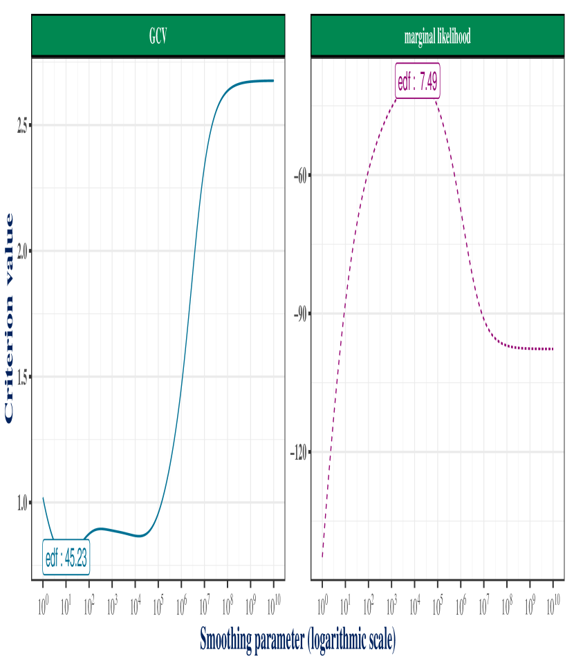
Figure 3 shows the values of GCV and marginal likelihood as a function of the smoothing parameter for the data used to produce Figure 1. When the marginal likelihood exhibits a clearly defined optimum, GCV has two optima, one of which coincides with the marginal likelihood’s optimum. The second optimum results in a model with nearly 45 degrees of freedom, which is not a plausible choice for the underlying mortality risk. For these reasons, we will favor the marginal likelihood as the selection criterion, especially since this choice naturally fits into the Bayesian framework introduced in Sections 2 and 4.

We will first discuss the selection in the case of the original Whittaker-Henderson smoothing and then extend the selection to the generalized case introduced in Section 4, introducing two competing approaches that will be subsequently compared.
Refer to caption
Figure 3: Comparison, in the context of one-dimensional Whittaker-Henderson smoothing, of the Generalized Cross-Validation (GCV) criterion and the marginal likelihood, as selection criteria for the smoothing parameter.

5.1 Selection in the context of the original smoothing

Let us start from the notations and assumptions from Section 2, namely 𝐲|𝜽𝒩(𝜽,W)similar-toconditional𝐲𝜽𝒩𝜽superscript𝑊\mathbf{y}|\boldsymbol{\theta}\sim\mathcal{N}(\boldsymbol{\theta},W^{-}) and 𝜽|λ𝒩(0,Pλ)similar-toconditional𝜽𝜆𝒩0superscriptsubscript𝑃𝜆\boldsymbol{\theta}|\lambda\sim\mathcal{N}(0,P_{\lambda}^{-}). In a purely Bayesian approach, it would be necessary to define a prior distribution on λ𝜆\lambda and then estimate the posterior distribution of each parameter vector using methods such as Markov Chain Monte Carlo. The empirical Bayesian approach we adopt seeks to find the value of λ𝜆\lambda that maximizes the marginal likelihood:

normm(λ)=f(𝐲|λ)=f(𝐲,𝜽|λ)d𝜽=f(𝐲|𝜽)f(𝜽|λ)d𝜽.subscriptsuperscript𝑚norm𝜆𝑓conditional𝐲𝜆𝑓𝐲conditional𝜽𝜆d𝜽𝑓conditional𝐲𝜽𝑓conditional𝜽𝜆d𝜽\mathcal{L}^{m}_{\text{norm}}(\lambda)=f(\mathbf{y}|\lambda)=\int f(\mathbf{y},\boldsymbol{\theta}|\lambda)\text{d}\boldsymbol{\theta}=\int f(\mathbf{y}|\boldsymbol{\theta})f(\boldsymbol{\theta}|\lambda)\text{d}\boldsymbol{\theta}.

This corresponds to the maximum likelihood method applied to the smoothing parameter. Let us explicitly rewrite the expressions of f(𝐲|𝜽)𝑓conditional𝐲𝜽f(\mathbf{y}|\boldsymbol{\theta}) and f(𝜽|λ)𝑓conditional𝜽𝜆f(\boldsymbol{\theta}|\lambda) introduced in Section 2:

f(𝐲|𝜽)𝑓conditional𝐲𝜽\displaystyle f(\mathbf{y}|\boldsymbol{\theta}) =|W|+(2π)nexp(12(𝐲𝜽)TW(𝐲𝜽))absentsubscript𝑊superscript2𝜋subscript𝑛12superscript𝐲𝜽𝑇𝑊𝐲𝜽\displaystyle=\sqrt{\frac{|W|_{+}}{(2\pi)^{n_{*}}}}\exp\left(-\frac{1}{2}(\mathbf{y}-\boldsymbol{\theta})^{T}W(\mathbf{y}-\boldsymbol{\theta})\right)
f(𝜽|λ)𝑓conditional𝜽𝜆\displaystyle f(\boldsymbol{\theta}|\lambda) =|Pλ|+(2π)pqexp(12𝜽TPλ𝜽)absentsubscriptsubscript𝑃𝜆superscript2𝜋𝑝𝑞12superscript𝜽𝑇subscript𝑃𝜆𝜽\displaystyle=\sqrt{\frac{|P_{\lambda}|_{+}}{(2\pi)^{p-q}}}\exp\left(-\frac{1}{2}\boldsymbol{\theta}^{T}P_{\lambda}\boldsymbol{\theta}\right)

where |A|+subscript𝐴|A|_{+} denotes the product of the non-zero eigenvalues of A𝐴A, nsubscript𝑛n_{*} is the number of non-zero diagonal elements of W𝑊W, and q𝑞q is the number of zero eigenvalues of Pλsubscript𝑃𝜆P_{\lambda} (q=qx×qz𝑞subscript𝑞𝑥subscript𝑞𝑧q=q_{x}\times q_{z} in the two-dimensional case). Based on the Taylor expansion performed in Section 2, let us recall that:

lnf(𝐲,𝜽|λ)=lnf(𝐲,𝜽^λ|λ)+12(𝜽𝜽^λ)T(W+Pλ)(𝜽𝜽^λ)𝑓𝐲conditional𝜽𝜆𝑓𝐲conditionalsubscript^𝜽𝜆𝜆12superscript𝜽subscript^𝜽𝜆𝑇𝑊subscript𝑃𝜆𝜽subscript^𝜽𝜆\ln f(\mathbf{y},\boldsymbol{\theta}|\lambda)=\ln f(\mathbf{y},\hat{\boldsymbol{\theta}}_{\lambda}|\lambda)+\frac{1}{2}(\boldsymbol{\theta}-\hat{\boldsymbol{\theta}}_{\lambda})^{T}(W+P_{\lambda})(\boldsymbol{\theta}-\hat{\boldsymbol{\theta}}_{\lambda})

which leads to:

normm(λ)subscriptsuperscript𝑚norm𝜆\displaystyle\mathcal{L}^{m}_{\text{norm}}(\lambda) =exp[lnf(𝐲,𝜽|λ)]d𝜽absent𝑓𝐲conditional𝜽𝜆d𝜽\displaystyle=\int\exp[\ln f(\mathbf{y},\boldsymbol{\theta}|\lambda)]\text{d}\boldsymbol{\theta}
=f(𝐲,𝜽^λ|λ)exp[12(𝜽𝜽^λ)T(W+Pλ)(𝜽𝜽^λ)]d𝜽absent𝑓𝐲conditionalsubscript^𝜽𝜆𝜆12superscript𝜽subscript^𝜽𝜆𝑇𝑊subscript𝑃𝜆𝜽subscript^𝜽𝜆d𝜽\displaystyle=f(\mathbf{y},\hat{\boldsymbol{\theta}}_{\lambda}|\lambda)\int\exp\left[-\frac{1}{2}(\boldsymbol{\theta}-\hat{\boldsymbol{\theta}}_{\lambda})^{T}(W+P_{\lambda})(\boldsymbol{\theta}-\hat{\boldsymbol{\theta}}_{\lambda})\right]\text{d}\boldsymbol{\theta}
=f(𝐲,𝜽^λ|λ)(2π)p|W+Pλ|absent𝑓𝐲conditionalsubscript^𝜽𝜆𝜆superscript2𝜋𝑝𝑊subscript𝑃𝜆\displaystyle=f(\mathbf{y},\hat{\boldsymbol{\theta}}_{\lambda}|\lambda)\sqrt{\frac{(2\pi)^{p}}{|W+P_{\lambda}|}}
=f𝐲(𝐲|𝜽^λ)f𝜽(𝜽^λ|λ)(2π)p|W+Pλ|absentsubscript𝑓𝐲conditional𝐲subscript^𝜽𝜆subscript𝑓𝜽conditionalsubscript^𝜽𝜆𝜆superscript2𝜋𝑝𝑊subscript𝑃𝜆\displaystyle=f_{\mathbf{y}}(\mathbf{y}|\hat{\boldsymbol{\theta}}_{\lambda})f_{\boldsymbol{\theta}}(\hat{\boldsymbol{\theta}}_{\lambda}|\lambda)\sqrt{\frac{(2\pi)^{p}}{|W+P_{\lambda}|}}
=|W|+|Pλ|+(2π)nq|W+Pλ|exp(12[(𝐲𝜽^λ)TW(𝐲𝜽^λ)+𝜽^λTPλ𝜽^λ]).absentsubscript𝑊subscriptsubscript𝑃𝜆superscript2𝜋subscript𝑛𝑞𝑊subscript𝑃𝜆12delimited-[]superscript𝐲subscript^𝜽𝜆𝑇𝑊𝐲subscript^𝜽𝜆superscriptsubscript^𝜽𝜆𝑇subscript𝑃𝜆subscript^𝜽𝜆\displaystyle=\sqrt{\frac{|W|_{+}|P_{\lambda}|_{+}}{(2\pi)^{n_{*}-q}|W+P_{\lambda}|}}\exp\left(-\frac{1}{2}\left[(\mathbf{y}-\hat{\boldsymbol{\theta}}_{\lambda})^{T}W(\mathbf{y}-\hat{\boldsymbol{\theta}}_{\lambda})+\hat{\boldsymbol{\theta}}_{\lambda}^{T}P_{\lambda}\hat{\boldsymbol{\theta}}_{\lambda}\right]\right).

The associated log-likelihood can be expressed as follows:

normm(λ)=12subscriptsuperscript𝑚norm𝜆12\displaystyle\ell^{m}_{\text{norm}}(\lambda)=-\frac{1}{2} [(𝐲𝜽^λ)TW(𝐲𝜽^λ)+𝜽^λTPλ𝜽^λ\displaystyle\left[(\mathbf{y}-\hat{\boldsymbol{\theta}}_{\lambda})^{T}W(\mathbf{y}-\hat{\boldsymbol{\theta}}_{\lambda})+\hat{\boldsymbol{\theta}}_{\lambda}^{T}P_{\lambda}\hat{\boldsymbol{\theta}}_{\lambda}\right. (12)
ln|W|+ln|Pλ|++ln|W+Pλ|+(nq)ln(2π)].\displaystyle\left.-\ln|W|_{+}-\ln|P_{\lambda}|_{+}+\ln|W+P_{\lambda}|+(n_{*}-q)\ln(2\pi)\right].

Once the selection of λ𝜆\lambda has been determined using the estimator λ^=argmax𝜆normm(λ)^𝜆𝜆argmaxsubscriptsuperscript𝑚norm𝜆\hat{\lambda}=\underset{\lambda}{\text{argmax}}\>\ell^{m}_{\text{norm}}(\lambda), the lack of an explicit solution to Equation 12 forces us to resort to numerical methods for its resolution. The Newton algorithm could once again be employed here and is a robust choice. This approach was notably adopted by Wood (2011). However, explicitly calculating the derivatives of the likelihood normmsubscriptsuperscript𝑚norm\ell^{m}_{\text{norm}} is rather difficult from an operational perspective. Instead, we will use general heuristics such as those provided by Brent (1973) and John A. Nelder and Mead (1965), which are applicable to any sufficiently smooth function. These heuristics do not require derivative calculations and are implemented in the optimize and optim functions of the statistical programming language 𝖱𝖱\mathsf{R}.

Computing the marginal likelihood using Equation 12 requires the estimation of various intermediate quantities, with the most demanding being the estimation of 𝜽^λsubscript^𝜽𝜆\hat{\boldsymbol{\theta}}_{\lambda}. This estimation is based on Equation 3 and ideally involves the inversion of the symmetric matrix W+Pλ𝑊subscript𝑃𝜆W+P_{\lambda} through a Cholesky decomposition. The calculation of ln|W+Pλ|𝑊subscript𝑃𝜆\ln|W+P_{\lambda}| is immediate for the triangular matrices resulting from this decomposition. Note that since the matrix Pλsubscript𝑃𝜆P_{\lambda} is a linear combination of the matrix Dn,qTDn,qsuperscriptsubscript𝐷𝑛𝑞𝑇subscript𝐷𝑛𝑞D_{n,q}^{T}D_{n,q} in the one-dimensional case, and the matrices InzDnx,qxTDnx,qxtensor-productsubscript𝐼subscript𝑛𝑧superscriptsubscript𝐷subscript𝑛𝑥subscript𝑞𝑥𝑇subscript𝐷subscript𝑛𝑥subscript𝑞𝑥I_{n_{z}}\otimes D_{n_{x},q_{x}}^{T}D_{n_{x},q_{x}} and Dnz,qzTDnz,qzInxtensor-productsuperscriptsubscript𝐷subscript𝑛𝑧subscript𝑞𝑧𝑇subscript𝐷subscript𝑛𝑧subscript𝑞𝑧subscript𝐼subscript𝑛𝑥D_{n_{z},q_{z}}^{T}D_{n_{z},q_{z}}\otimes I_{n_{x}} in the two-dimensional case, it is only necessary to form these matrices once. Furthermore, the calculation of ln|Pλ|+subscriptsubscript𝑃𝜆\ln|P_{\lambda}|_{+} can be efficiently performed by computing the eigendecomposition of the matrix Dn,qTDn,qsuperscriptsubscript𝐷𝑛𝑞𝑇subscript𝐷𝑛𝑞D_{n,q}^{T}D_{n,q} (or the matrices Dnx,qxTDnx,qxsuperscriptsubscript𝐷subscript𝑛𝑥subscript𝑞𝑥𝑇subscript𝐷subscript𝑛𝑥subscript𝑞𝑥D_{n_{x},q_{x}}^{T}D_{n_{x},q_{x}} and Dnz,qzTDnz,qzsuperscriptsubscript𝐷subscript𝑛𝑧subscript𝑞𝑧𝑇subscript𝐷subscript𝑛𝑧subscript𝑞𝑧D_{n_{z},q_{z}}^{T}D_{n_{z},q_{z}} in the two-dimensional case). This calculation then only requires multiplying these eigenvalues by the corresponding element of λ𝜆\lambda and taking the logarithm. Finally, since the terms ln|W|+subscript𝑊\ln|W|_{+} and (nq)ln(2π)subscript𝑛𝑞2𝜋(n_{*}-q)\ln(2\pi) do not depend on λ𝜆\lambda, they can be ignored altogether.

5.2 Selection in the generalized smoothing framework: outer iteration approach

It is possible to extend the previous approach to the framework of penalized likelihood introduced in Section 4. The Taylor expansion used in Section 5.1 can be applied in this context and yields:

MLm(λ)subscriptsuperscript𝑚ML𝜆\displaystyle\mathcal{L}^{m}_{\text{ML}}(\lambda) =exp[lnf(𝐝,𝐞𝐜,𝜽|λ)]d𝜽absent𝑓𝐝subscript𝐞𝐜conditional𝜽𝜆d𝜽\displaystyle=\int\exp[\ln f(\mathbf{d},\mathbf{e_{c}},\boldsymbol{\theta}|\lambda)]\text{d}\boldsymbol{\theta}
f(𝐝,𝐞𝐜,𝜽^λ|λ)exp(12(𝜽𝜽^λ)T(W𝜽^λ+Pλ)(𝜽𝜽^λ))d𝜽similar-to-or-equalsabsent𝑓𝐝subscript𝐞𝐜conditionalsubscript^𝜽𝜆𝜆12superscript𝜽subscript^𝜽𝜆𝑇subscript𝑊subscript^𝜽𝜆subscript𝑃𝜆𝜽subscript^𝜽𝜆d𝜽\displaystyle\simeq f(\mathbf{d},\mathbf{e_{c}},\hat{\boldsymbol{\theta}}_{\lambda}|\lambda)\int\exp\left(-\frac{1}{2}(\boldsymbol{\theta}-\hat{\boldsymbol{\theta}}_{\lambda})^{T}(W_{\hat{\boldsymbol{\theta}}_{\lambda}}+P_{\lambda})(\boldsymbol{\theta}-\hat{\boldsymbol{\theta}}_{\lambda})\right)\text{d}\boldsymbol{\theta}
f(𝐝,𝐞𝐜,𝜽^λ|λ)(2π)p|W𝜽^λ+Pλ|similar-to-or-equalsabsent𝑓𝐝subscript𝐞𝐜conditionalsubscript^𝜽𝜆𝜆superscript2𝜋𝑝subscript𝑊subscript^𝜽𝜆subscript𝑃𝜆\displaystyle\simeq f(\mathbf{d},\mathbf{e_{c}},\hat{\boldsymbol{\theta}}_{\lambda}|\lambda)\sqrt{\frac{(2\pi)^{p}}{|W_{\hat{\boldsymbol{\theta}}_{\lambda}}+P_{\lambda}|}}
l(𝜽^λ)f𝜽(𝜽^λ|λ)(2π)p|W𝜽^λ+Pλ|similar-to-or-equalsabsent𝑙subscript^𝜽𝜆subscript𝑓𝜽conditionalsubscript^𝜽𝜆𝜆superscript2𝜋𝑝subscript𝑊subscript^𝜽𝜆subscript𝑃𝜆\displaystyle\simeq l(\hat{\boldsymbol{\theta}}_{\lambda})f_{\boldsymbol{\theta}}(\hat{\boldsymbol{\theta}}_{\lambda}|\lambda)\sqrt{\frac{(2\pi)^{p}}{|W_{\hat{\boldsymbol{\theta}}_{\lambda}}+P_{\lambda}|}}
l(𝜽^λ)(2π)q|Pλ|+|W𝜽^λ+Pλ|exp(12𝜽^λTPλ𝜽^λ).similar-to-or-equalsabsent𝑙subscript^𝜽𝜆superscript2𝜋𝑞subscriptsubscript𝑃𝜆subscript𝑊subscript^𝜽𝜆subscript𝑃𝜆12superscriptsubscript^𝜽𝜆𝑇subscript𝑃𝜆subscript^𝜽𝜆\displaystyle\simeq l(\hat{\boldsymbol{\theta}}_{\lambda})\sqrt{\frac{(2\pi)^{q}|P_{\lambda}|_{+}}{|W_{\hat{\boldsymbol{\theta}}_{\lambda}}+P_{\lambda}|}}\exp\left(-\frac{1}{2}\hat{\boldsymbol{\theta}}_{\lambda}^{T}P_{\lambda}\hat{\boldsymbol{\theta}}_{\lambda}\right).

This gives us the expression for the likelihood in this framework:

MLm(λ)l(𝜽^λ)12[𝜽^λTPλ𝜽^λln|Pλ|++ln|W𝜽^λ+Pλ|qln(2π)].subscriptsuperscript𝑚ML𝜆𝑙subscript^𝜽𝜆12delimited-[]superscriptsubscript^𝜽𝜆𝑇subscript𝑃𝜆subscript^𝜽𝜆subscriptsubscript𝑃𝜆subscript𝑊subscript^𝜽𝜆subscript𝑃𝜆𝑞2𝜋\hypertarget{eq-REML2}{}{\ell^{m}_{\text{ML}}(\lambda)\approx l(\hat{\boldsymbol{\theta}}_{\lambda})-\frac{1}{2}\left[\hat{\boldsymbol{\theta}}_{\lambda}^{T}P_{\lambda}\hat{\boldsymbol{\theta}}_{\lambda}-\ln|P_{\lambda}|_{+}+\ln|W_{\hat{\boldsymbol{\theta}}_{\lambda}}+P_{\lambda}|-q\ln(2\pi)\right].} (13)

Unlike the normal case, the Taylor expansion does not allow for an exact calculation of the marginal likelihood but provides an approximation known as the Laplace approximation, whose validity depends on the number of available observations. Equation 13 does not have an explicit solution and requires numerical resolution. The calculation of the Laplace approximation of the marginal likelihood is done in a similar manner to Equation 12 from Section 5.1, with the only notable difference being that the vector 𝜽^λsubscript^𝜽𝜆\hat{\boldsymbol{\theta}}_{\lambda} must be estimated iteratively using Algorithm 1. This leads to Algorithm 2 for selecting the smoothing parameter which includes two nested iterative calculations: the calculation of 𝜽^λsubscript^𝜽𝜆\hat{\boldsymbol{\theta}}_{\lambda}, for a fixed λ𝜆\lambda, using the Newton algorithm, and the search for the maximum of MLmsubscriptsuperscript𝑚ML\ell^{m}_{\text{ML}} using heuristics such as the Brent and Nelder-Mead algorithms in the one-dimensional and two-dimensional case, respectively. Since the selection of λ𝜆\lambda corresponds to the outer iterative loop here, and to distinguish it from the approach introduced in the next section, we will refer to it as the outer iteration approach.

inputs : 𝐝𝐝\mathbf{d} and 𝐞𝐜subscript𝐞𝐜\mathbf{e_{c}}
outputs : λ^^𝜆\hat{\lambda}, 𝜽^λ^subscript^𝜽^𝜆\hat{\boldsymbol{\theta}}_{\hat{\lambda}} and Var(𝜽^λ^)Varsubscript^𝜽^𝜆\text{Var}(\hat{\boldsymbol{\theta}}_{\hat{\lambda}})
parameters : q𝑞q, ϵ=108subscriptitalic-ϵsuperscript108\epsilon_{\ell}=10^{-8}, ϵml=108subscriptitalic-ϵmlsuperscript108\epsilon_{\text{ml}}=10^{-8}
begin
       k0𝑘0k\leftarrow 0
       ml0,condmltrueformulae-sequencesubscriptml0subscriptcondmltrue\text{ml}_{0}\leftarrow-\infty,\quad\text{cond}_{\text{ml}}\leftarrow\text{true}
       while condmlsubscriptcondml\text{cond}_{\text{ml}} do
             If k=0𝑘0k=0, choose an arbitrary value λ0subscript𝜆0\lambda_{0} for the smoothing parameter(s); otherwise, choose the next value λksubscript𝜆𝑘\lambda_{k} using the selected heuristic
             Use Algorithm 1 to determine the vector 𝜽λksubscript𝜽subscript𝜆𝑘\boldsymbol{\theta}_{\lambda_{k}} associated with the choice of λksubscript𝜆𝑘\lambda_{k} with an accuracy greater than ϵsubscriptitalic-ϵ\epsilon_{\ell}
             Calculate the marginal likelihood MLm(λk)subscriptsuperscript𝑚MLsubscript𝜆𝑘\ell^{m}_{\text{ML}}(\lambda_{k}) associated with the choice of λksubscript𝜆𝑘\lambda_{k} using the intermediate quantities calculated during the estimation of 𝜽λksubscript𝜽subscript𝜆𝑘\boldsymbol{\theta}_{\lambda_{k}}
             mlk+1MLm(λk),condmlmlk+1mlkϵml×sum(d)formulae-sequencesubscriptml𝑘1subscriptsuperscript𝑚MLsubscript𝜆𝑘subscriptcondmlsubscriptml𝑘1subscriptml𝑘subscriptitalic-ϵmlsum𝑑\text{ml}_{k+1}\leftarrow\ell^{m}_{\text{ML}}(\lambda_{k}),\quad\text{cond}_{\text{ml}}\leftarrow\text{ml}_{k+1}-\text{ml}_{k}\geq\epsilon_{\text{ml}}\times\text{sum}(d)
             kk+1𝑘𝑘1k\leftarrow k+1
            
      𝜽^𝜽^λ^,Var(𝜽^)Ψkformulae-sequence^𝜽subscript^𝜽^𝜆Var^𝜽subscriptΨ𝑘\hat{\boldsymbol{\theta}}\leftarrow\hat{\boldsymbol{\theta}}_{\hat{\lambda}},\quad\text{Var}(\hat{\boldsymbol{\theta}})\leftarrow\Psi_{k}
      
Algorithm 2 Parameter selection for generalized Whittaker-Henderson smoothing - outer iteration approach.

5.3 Selection in the generalized smoothing framework: performance iteration approach

An alternative to the approach developed in Section 5.2 is to start from Algorithm 1 and notice that at each step of the algorithm, the solved equations coincide with those obtained by assuming that 𝐳k|𝜽𝒩(𝜽,Wk1)similar-toconditionalsubscript𝐳𝑘𝜽𝒩𝜽superscriptsubscript𝑊𝑘1\mathbf{z}_{k}|\boldsymbol{\theta}\sim\mathcal{N}(\boldsymbol{\theta},W_{k}^{-1}) and 𝜽𝒩(0,Pλ)similar-to𝜽𝒩0superscriptsubscript𝑃𝜆\boldsymbol{\theta}\sim\mathcal{N}(0,P_{\lambda}^{-}). Therefore, it is possible to rely on the methodology proposed in Section 5.1 and numerically estimate, at the beginning of each iteration of Algorithm 1, the smoothing parameter that maximizes the marginal likelihood normmsubscriptsuperscript𝑚norm\ell^{m}_{\text{norm}} in which 𝐲𝐲\mathbf{y} would be replaced by 𝐳ksubscript𝐳𝑘\mathbf{z}_{k} and W𝑊W by Wksubscript𝑊𝑘W_{k}. This is what Algorithm 3 proposes. A justification for this approach is given by (Wood 2006, p149). From a practical point of view, this approach conceptually reverses the nesting order of the two types of iterations and can, in some cases, provide a considerable time gain. It was introduced by Gu (1992) as the “performance (oriented) iteration” approach. However, unlike the outer iteration approach, the convergence of the performance iteration approach cannot be guaranteed. Indeed, the penalized likelihood calculated in Algorithm 3 is not directly comparable between iterations because it is based on a different smoothing parameter and, therefore, a different prior. There are situations in which this algorithm may not converge. However, this difficulty seems to be more of a theoretical nature than a practical one for the optimization problem addressed in this paper.

inputs : 𝐝𝐝\mathbf{d} and 𝐞𝐜subscript𝐞𝐜\mathbf{e_{c}}
outputs : λ^^𝜆\hat{\lambda}, 𝜽^λ^subscript^𝜽^𝜆\hat{\boldsymbol{\theta}}_{\hat{\lambda}} and Var(𝜽^λ^)Varsubscript^𝜽^𝜆\text{Var}(\hat{\boldsymbol{\theta}}_{\hat{\lambda}})
parameters : q𝑞q, ϵ=108subscriptitalic-ϵsuperscript108\epsilon_{\ell}=10^{-8}, ϵml=108subscriptitalic-ϵmlsuperscript108\epsilon_{\text{ml}}=10^{-8}
begin
       k0𝑘0k\leftarrow 0
       𝜽0ln(𝐝/𝐞𝐜)subscript𝜽0𝐝subscript𝐞𝐜\boldsymbol{\theta}_{0}\leftarrow\ln(\mathbf{d}/\mathbf{e_{c}})
       l0,condtrueformulae-sequencesubscript𝑙0subscriptcondtruel_{0}\leftarrow-\infty,\quad\text{cond}_{\ell}\leftarrow\text{true}
       while condsubscriptcond\text{cond}_{\ell} do
             WkDiag(𝐞𝐱𝐩(𝜽k)𝐞𝐜)subscript𝑊𝑘Diagdirect-productsubscript𝜽𝑘subscript𝐞𝐜W_{k}\leftarrow\text{Diag}(\boldsymbol{\exp}(\boldsymbol{\theta}_{k})\odot\mathbf{e_{c}})
             𝐳k𝜽k+Wk1[𝐝𝐞𝐱𝐩(𝜽k)𝐞𝐜]subscript𝐳𝑘subscript𝜽𝑘superscriptsubscript𝑊𝑘1delimited-[]𝐝direct-productsubscript𝜽𝑘subscript𝐞𝐜\mathbf{z}_{k}\leftarrow\boldsymbol{\theta}_{k}+W_{k}^{-1}[\mathbf{d}-\boldsymbol{\exp}(\boldsymbol{\theta}_{k})\odot\mathbf{e_{c}}]
             Estimate the parameter λksubscript𝜆𝑘\lambda_{k} maximizing the regularized marginal likelihood normmsubscriptsuperscript𝑚norm\ell^{m}_{\text{norm}} associated with the observation vector 𝐳k𝐳𝑘\mathbf{z}k and the weight matrix Wksubscript𝑊𝑘W_{k}, using the selected heuristic, with an accuracy greater than ϵml×sum(d)subscriptitalic-ϵmlsum𝑑\epsilon_{\text{ml}}\times\text{sum}(d)
             Ψk+1(Wk+Pλk)1subscriptΨ𝑘1superscriptsubscript𝑊𝑘subscript𝑃subscript𝜆𝑘1\Psi_{k+1}\leftarrow(W_{k}+P_{\lambda_{k}})^{-1}
             𝜽k+1Ψk+1Wk𝐳ksubscript𝜽𝑘1subscriptΨ𝑘1subscript𝑊𝑘subscript𝐳𝑘\boldsymbol{\theta}_{k+1}\leftarrow\Psi_{k+1}W_{k}\mathbf{z}_{k}
             lk+1P(𝜽k+1|λk),condlk+1lkϵ×sum(d)formulae-sequencesubscript𝑙𝑘1subscript𝑃conditionalsubscript𝜽𝑘1subscript𝜆𝑘subscriptcondsubscript𝑙𝑘1subscript𝑙𝑘subscriptitalic-ϵsum𝑑l_{k+1}\leftarrow\ell_{P}(\boldsymbol{\theta}_{k+1}|\lambda_{k}),\quad\text{cond}_{\ell}\leftarrow l_{k+1}-l_{k}\geq\epsilon_{\ell}\times\text{sum}(d)
             kk+1𝑘𝑘1k\leftarrow k+1
            
      λ^λk^𝜆subscript𝜆𝑘\hat{\lambda}\leftarrow\lambda_{k}; Use Algorithm 1 to obtain the values of 𝜽^λ^subscript^𝜽^𝜆\hat{\boldsymbol{\theta}}_{\hat{\lambda}} and Var(𝜽^λ^)Varsubscript^𝜽^𝜆\text{Var}(\hat{\boldsymbol{\theta}}_{\hat{\lambda}}) corresponding to the parameter λ^^𝜆\hat{\lambda}
      
Algorithm 3 Parameter selection for generalized Whittaker-Henderson smoothing - performance iteration approach

5.4 Comparison of outer iteration and performance iteration approaches

In Sections 5.2 and 5.3, we introduced two alternatives for the selection of parameters in generalized Whittaker-Henderson smoothing. This section aims to study the consequences of choosing one approach over the other in terms of result accuracy and computational time. While the objective of Section 4.2 was to highlight a bias in the asymptotic approximation associated with the original Whittaker-Henderson smoothing for small portfolios, here we aim to measure these impacts more precisely. We limit our analysis to intermediate-sized portfolios as presented in Section 4.2 (i.e., 100,000 rows for the one-dimensional case and 5,000 rows for the two-dimensional case), but we use 100 replicates of each portfolio, generated from the same mortality and censoring laws, to increase the robustness of our analysis.

The outer iteration and performance iteration approaches can be directly compared based on the selected parameter λ𝜆\lambda and using the marginal likelihood MLm(λ)subscriptsuperscript𝑚ML𝜆\ell^{m}_{\text{ML}}(\lambda). Similar to Section 4.2, we define the error criterion as:

Δ(λ)=MLm(λ^outer)MLm(λ)MLm(λ^outer)MLm()Δ𝜆subscriptsuperscript𝑚MLsubscript^𝜆outersubscriptsuperscript𝑚ML𝜆subscriptsuperscript𝑚MLsubscript^𝜆outersubscriptsuperscript𝑚ML\hypertarget{eq-delta2}{}{\Delta(\lambda)=\frac{\ell^{m}_{\text{ML}}(\hat{\lambda}_{\text{outer}})-\ell^{m}_{\text{ML}}(\lambda)}{\ell^{m}_{\text{ML}}(\hat{\lambda}_{\text{outer}})-\ell^{m}_{\text{ML}}(\infty)}} (14)

where MLm()subscriptsuperscript𝑚ML\ell^{m}_{\text{ML}}(\infty) corresponds to the approximation of the marginal likelihood associated with the choice of an infinite smoothing parameter. Again, the defined ΔΔ\Delta satisfies the properties Δ(λouter)=0Δsubscript𝜆outer0\Delta(\lambda_{\text{outer}})=0 and Δ()=1Δ1\Delta(\infty)=1. This criterion is interpreted in the same way as the one given by Equation 11.
Refer to caption
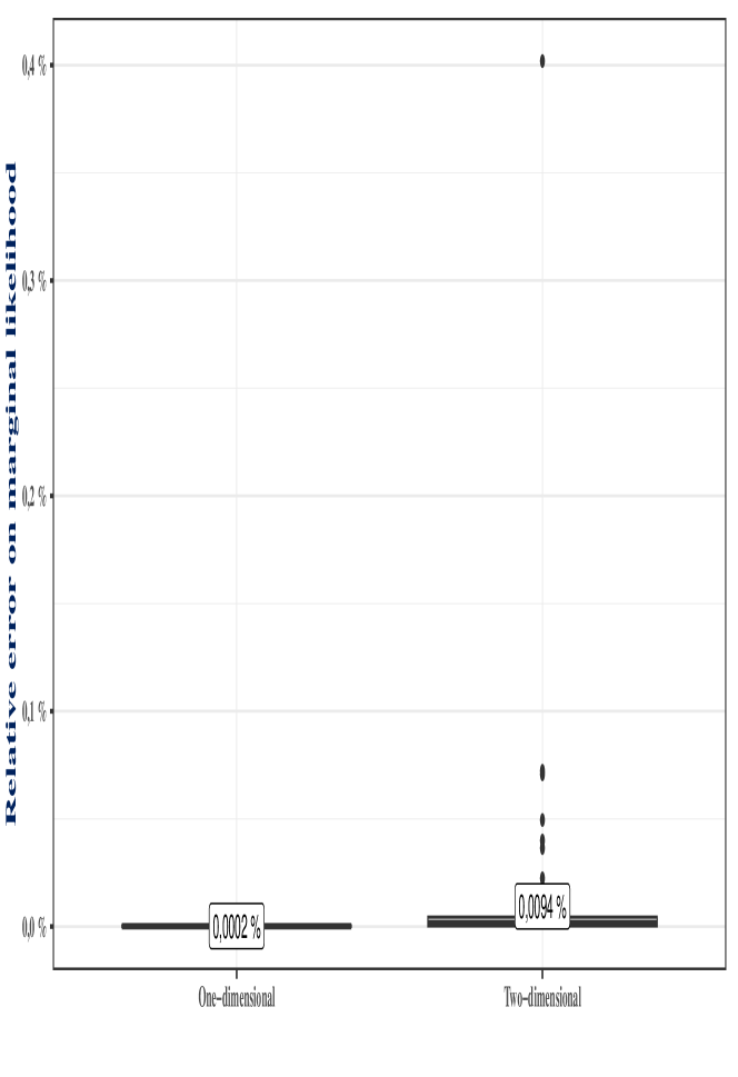
Figure 4: Distribution of the difference between the two presented approaches for selecting the smoothing parameter, for 100 simulated portfolios, in the one-dimensional and two-dimensional case.

Figure 4 represents the empirical distribution of the difference between the outer iteration and performance iteration approaches, and Figure 5 represents the distribution of the associated computation time for each approach. The use of the performance iteration approach results in a difference below 1% for the 100 simulated datasets, both in the one-dimensional and two-dimensional case. The associated computation time is reduced by a factor of 2 in the one-dimensional case and nearly 4 in the two-dimensional case. Considering the significant computation times in the latter case, the use of the performance iteration approach presents a real operational advantage.
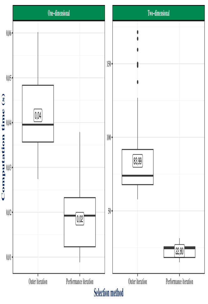
Refer to caption
Figure 5: Distribution of the computation time associated with the two presented approaches for selecting the smoothing parameter, for 100 simulated portfolios, in the one-dimensional and two-dimensional case.

6 How to improve smoothing performances with a large number of data points?

6.1 Motivation

Whittaker-Henderson smoothing is considered to be full-rank smoothing as it contains as many parameters as there are observation points. This characteristic allows it to faithfully reproduce any input signal, provided that a sufficient number of observations are available. More formally, the estimator associated with smoothing is asymptotically unbiased since:

𝔼(𝐲^)=(W+Pλ)1W𝔼(𝐲)m𝔼(𝐲)𝔼^𝐲superscript𝑊subscript𝑃𝜆1𝑊𝔼𝐲𝑚𝔼𝐲\mathbb{E}(\hat{\mathbf{y}})=(W+P_{\lambda})^{-1}W\mathbb{E}(\mathbf{y})\underset{m\rightarrow\infty}{\rightarrow}\mathbb{E}(\mathbf{y})

where m𝑚m represents the number of observed individuals and is involved in the matrix W𝑊W. The downside is that it may become impractical in presence of many observations points n𝑛n. Indeed, the algorithms presented in Section 5 require the inversion of the n×n𝑛𝑛n\times n matrix W+Pλ𝑊subscript𝑃𝜆W+P_{\lambda}, an operation with a time complexity of O(n3)𝑂superscript𝑛3O(n^{3}), which needs to be repeated at each iteration of the algorithm, regardless of the chosen method.

For biometric risks that depend solely on age, discretized on an annual basis, the number of observations rarely exceeds 100, and computation time is not a significant concern. However, in the two-dimensional case, the number of observations can take much larger values in several practical cases, including:

  • \bullet

    For the disability risk, it is necessary to construct disability survival tables for entry ages ranging from 18 to 62 and exit ages ranging from the entry age to 62. This represents [(6218)×(6218+1)/2=990[(62-18)\times(62-18+1)/2=990 observations.

  • \bullet

    Also for the disability risk, it is necessary to construct transition tables from incapacity to disability for entry ages ranging from 18 to 67 and monthly incapacity durations ranging from 0 to 36 months. This represents (6718)×(360)=1,76467183601764(67-18)\times(36-0)=1,764 observations.

  • \bullet

    For the long-term care risk, as the coverage is lifelong, it is necessary to construct tables for all ages and long-term care durations encountered in the data. Assuming observation ages ranging from 50 to 110 and durations ranging from 0 to 20 years, this already represents (11050)×(200)=1,200110502001200(110-50)\times(20-0)=1,200 observations.

The practical applications described above thus require computation times on the order of several minutes for each smoothing application. When smoothing is intended to be used repeatedly, for example, in simulation contexts, reducing the computation time becomes an operational challenge.

6.2 Smoothing and eigendecomposition

The eigendecomposition of the penalization matrix is key to a better understanding of smoothing and allows for an approximation of the smoothing problem with p<n𝑝𝑛p<n parameters. Let us consider the one-dimensional case and write the decomposition for the symmetric matrix Dn,qTDn,qsuperscriptsubscript𝐷𝑛𝑞𝑇subscript𝐷𝑛𝑞D_{n,q}^{T}D_{n,q}. It takes the form Dn,qTDn,q=UΣUTsuperscriptsubscript𝐷𝑛𝑞𝑇subscript𝐷𝑛𝑞𝑈Σsuperscript𝑈𝑇D_{n,q}^{T}D_{n,q}=U\Sigma U^{T}, where ΣΣ\Sigma is a diagonal matrix containing the eigenvalues of Dn,qTDn,qsuperscriptsubscript𝐷𝑛𝑞𝑇subscript𝐷𝑛𝑞D_{n,q}^{T}D_{n,q} and U𝑈U is an orthogonal matrix such that UTU=UUT=Insuperscript𝑈𝑇𝑈𝑈superscript𝑈𝑇subscript𝐼𝑛U^{T}U=UU^{T}=I_{n}. Let us perform the reparameterization 𝜷=UT𝜽𝜽=U𝜷𝜷superscript𝑈𝑇𝜽𝜽𝑈𝜷\boldsymbol{\beta}=U^{T}\boldsymbol{\theta}\Leftrightarrow\boldsymbol{\theta}=U\boldsymbol{\beta}. The smoothness criterion becomes:

𝜽TPλ𝜽=(U𝜷)TPλ(U𝜷)=λ𝜷TUTUΣUTU𝜷=λ𝜷TΣ𝜷.superscript𝜽𝑇subscript𝑃𝜆𝜽superscript𝑈𝜷𝑇subscript𝑃𝜆𝑈𝜷𝜆superscript𝜷𝑇superscript𝑈𝑇𝑈Σsuperscript𝑈𝑇𝑈𝜷𝜆superscript𝜷𝑇Σ𝜷\hypertarget{eq-interpretation1}{}{\boldsymbol{\theta}^{T}P_{\lambda}\boldsymbol{\theta}=(U\boldsymbol{\beta})^{T}P_{\lambda}(U\boldsymbol{\beta})=\lambda\boldsymbol{\beta}^{T}U^{T}U\Sigma U^{T}U\boldsymbol{\beta}=\lambda\boldsymbol{\beta}^{T}\Sigma\boldsymbol{\beta}.} (15)

and Equation 2 takes the form:

𝐲^=U𝜷^where𝜷^=argmin𝜷{(𝐲U𝜷)TW(𝐲U𝜷)+λ𝜷TΣ𝜷}.formulae-sequence^𝐲𝑈^𝜷where^𝜷𝜷argminsuperscript𝐲𝑈𝜷𝑇𝑊𝐲𝑈𝜷𝜆superscript𝜷𝑇Σ𝜷\hypertarget{eq-interpretation2}{}{\hat{\mathbf{y}}=U\hat{\boldsymbol{\beta}}\quad\text{where}\quad\hat{\boldsymbol{\beta}}=\underset{\boldsymbol{\beta}}{\text{argmin}}\left\{(\mathbf{y}-U\boldsymbol{\beta})^{T}W(\mathbf{y}-U\boldsymbol{\beta})+\lambda\boldsymbol{\beta}^{T}\Sigma\boldsymbol{\beta}\right\}.} (16)

In the original formulation of smoothing, the parameters directly corresponded to the smoothed values. With this new parameterization, 𝜷𝜷\boldsymbol{\beta} can be interpreted as a vector of coordinates in the basis of eigenvectors of Pλsubscript𝑃𝜆P_{\lambda}, providing a decomposition of the signal into components that are more or less smooth according to the employed penalization. Figure 6 represents 8 of the eigenvectors associated with q=2𝑞2q=2 for a basis of size n=74𝑛74n=74, which corresponds to the number of observations in the mortality portfolio used, notably in Figure 1. The eigenvalues associated with the first q𝑞q eigenvalues are zero. This result can be easily explained by noting that Dn,qsubscript𝐷𝑛𝑞D_{n,q} is a matrix of dimensions (nq)×n𝑛𝑞𝑛(n-q)\times n and rank nq𝑛𝑞n-q.

Refer to caption
Figure 6: Graphical representation of a subset of columns from a basis of eigenvectors associated with n=74𝑛74n=74 and q=2𝑞2q=2 in the one-dimensional case. The 8 vectors in the subset are displayed in order of increasing penalization.

By using the fact that U1=UTsuperscript𝑈1superscript𝑈𝑇U^{-1}=U^{T} and making the connection with Equation 3, we obtain the explicit solution:

𝐲^=U(UTWU+Sλ)1UTW𝐲whereSλ=λΣformulae-sequence^𝐲𝑈superscriptsuperscript𝑈𝑇𝑊𝑈subscript𝑆𝜆1superscript𝑈𝑇𝑊𝐲wheresubscript𝑆𝜆𝜆Σ\hypertarget{eq-interpretation3}{}{\hat{\mathbf{y}}=U(U^{T}WU+S_{\lambda})^{-1}U^{T}W\mathbf{y}\quad\text{where}\quad S_{\lambda}=\lambda\Sigma} (17)

In order to interpret Equation 17, let us consider the special case where all weights are equal to 1, and we have:

𝐲^=U(UTU+λΣ)1UT𝐲=U(In+λΣ)1UT𝐲^𝐲𝑈superscriptsuperscript𝑈𝑇𝑈𝜆Σ1superscript𝑈𝑇𝐲𝑈superscriptsubscript𝐼𝑛𝜆Σ1superscript𝑈𝑇𝐲\hat{\mathbf{y}}=U(U^{T}U+\lambda\Sigma)^{-1}U^{T}\mathbf{y}=U(I_{n}+\lambda\Sigma)^{-1}U^{T}\mathbf{y}

The transformation from 𝐲𝐲\mathbf{y} to 𝐲^^𝐲\hat{\mathbf{y}} can then be seen as a three-step process, reading the equation from right to left:

  1. 1.

    Decomposition of the signal 𝐲𝐲\mathbf{y} in the basis of eigenvectors through the left multiplication by UTsuperscript𝑈𝑇U^{T}.

  2. 2.

    Attenuation of the signal components based on the eigenvalues associated with these components. If we denote s=diag(Σ)𝑠diagΣs=\text{diag}(\Sigma), then (In+λΣ)1=Diag[1/(1+λs)]superscriptsubscript𝐼𝑛𝜆Σ1Diagdelimited-[]11𝜆𝑠(I_{n}+\lambda\Sigma)^{-1}=\text{Diag}[1/(1+\lambda s)]. After the left multiplication by (In+λΣ)1superscriptsubscript𝐼𝑛𝜆Σ1(I_{n}+\lambda\Sigma)^{-1}, each component is divided by a coefficient 1+λs11𝜆𝑠11+\lambda s\geq 1. This attenuation coefficient increases linearly with λ𝜆\lambda, but at different rates for each eigenvalue.

  3. 3.

    Reconstruction of the attenuated signal in the canonical basis through the left multiplication by U𝑈U.

In the presence of non-unit weights, things are not as straightforward since UTWUsuperscript𝑈𝑇𝑊𝑈U^{T}WU is no longer a diagonal matrix. However, it is still possible to visualize the effect of smoothing by looking at the matrix F=(UTWU+Sλ)1UTWU𝐹superscriptsuperscript𝑈𝑇𝑊𝑈subscript𝑆𝜆1superscript𝑈𝑇𝑊𝑈F=(U^{T}WU+S_{\lambda})^{-1}U^{T}WU. In fact:

UT𝐲^=UTU𝜽^=𝜽^=(UTWU+Sλ)1UTW𝐲=(UTWU+Sλ)1UTWUUT𝐲=FUT𝐲superscript𝑈𝑇^𝐲superscript𝑈𝑇𝑈^𝜽^𝜽superscriptsuperscript𝑈𝑇𝑊𝑈subscript𝑆𝜆1superscript𝑈𝑇𝑊𝐲superscriptsuperscript𝑈𝑇𝑊𝑈subscript𝑆𝜆1superscript𝑈𝑇𝑊𝑈superscript𝑈𝑇𝐲𝐹superscript𝑈𝑇𝐲U^{T}\hat{\mathbf{y}}=U^{T}U\hat{\boldsymbol{\theta}}=\hat{\boldsymbol{\theta}}=(U^{T}WU+S_{\lambda})^{-1}U^{T}W\mathbf{y}=(U^{T}WU+S_{\lambda})^{-1}U^{T}WUU^{T}\mathbf{y}=FU^{T}\mathbf{y}

Since the vectors UT𝐲superscript𝑈𝑇𝐲U^{T}\mathbf{y} and 𝜷^=UT𝐲^^𝜷superscript𝑈𝑇^𝐲\hat{\boldsymbol{\beta}}=U^{T}\hat{\mathbf{y}} represent the coordinates of the signals 𝐲𝐲\mathbf{y} and 𝐲^^𝐲\hat{\mathbf{y}} in the basis of eigenvectors of Dn,qTDn,qsuperscriptsubscript𝐷𝑛𝑞𝑇subscript𝐷𝑛𝑞D_{n,q}^{T}D_{n,q}, F𝐹F corresponds to a coordinate transformation matrix playing a similar role for the parameters as the hat matrix H=U(UTWU+Sλ)1UTW𝐻𝑈superscriptsuperscript𝑈𝑇𝑊𝑈subscript𝑆𝜆1superscript𝑈𝑇𝑊H=U(U^{T}WU+S_{\lambda})^{-1}U^{T}W does for the observations. The diagonal values of F𝐹F can be interpreted as the effective degrees of freedom associated with each eigenvector after smoothing. It can be verified that:

tr(F)=tr[(UTWU+Sλ)1UTWU]=tr[U(UTWU+Sλ)1UTW]=tr(H)tr𝐹trdelimited-[]superscriptsuperscript𝑈𝑇𝑊𝑈subscript𝑆𝜆1superscript𝑈𝑇𝑊𝑈trdelimited-[]𝑈superscriptsuperscript𝑈𝑇𝑊𝑈subscript𝑆𝜆1superscript𝑈𝑇𝑊tr𝐻\text{tr}(F)=\text{tr}[(U^{T}WU+S_{\lambda})^{-1}U^{T}WU]=\text{tr}[U(U^{T}WU+S_{\lambda})^{-1}U^{T}W]=\text{tr}(H)

which means that the sum of the effective degrees of freedom remains the same whether it is counted per observation or per parameter.

Figure 7 represents the effective degrees of freedom per parameter in the previous illustration of smoothing. The first q𝑞q eigenvectors are never penalized, so their effective degrees of freedom are always equal to 1, regardless of the smoothing parameter used. The other eigenvectors have strictly decreasing effective degrees of freedom with λ𝜆\lambda. These degrees of freedom are generally decreasing with increasing eigenvalues of Dn,qTDn,qsuperscriptsubscript𝐷𝑛𝑞𝑇subscript𝐷𝑛𝑞D_{n,q}^{T}D_{n,q}, although in the presence of non-unit weights and for small values of λ𝜆\lambda, this may not always be the case.

Refer to caption
Figure 7: Distribution of residual degrees of freedom per eigenvector after applying the Whittaker-Henderson smoothing, in the one-dimensional case, for different values of the smoothing parameter.

6.3 Extension to the two-dimensional case

In the two-dimensional case, we have Pλ=λxInzDnx,qxTDnx,qx+λzDnz,qzTDnz,qzInxsubscript𝑃𝜆tensor-productsubscript𝜆𝑥subscript𝐼subscript𝑛𝑧superscriptsubscript𝐷subscript𝑛𝑥subscript𝑞𝑥𝑇subscript𝐷subscript𝑛𝑥subscript𝑞𝑥tensor-productsubscript𝜆𝑧superscriptsubscript𝐷subscript𝑛𝑧subscript𝑞𝑧𝑇subscript𝐷subscript𝑛𝑧subscript𝑞𝑧subscript𝐼subscript𝑛𝑥P_{\lambda}=\lambda_{x}I_{n_{z}}\otimes D_{n_{x},q_{x}}^{T}D_{n_{x},q_{x}}+\lambda_{z}D_{n_{z},q_{z}}^{T}D_{n_{z},q_{z}}\otimes I_{n_{x}}. Similar to the one-dimensional case, we can perform the eigendecomposition of the matrices Dnx,qxTDnx,qxsuperscriptsubscript𝐷subscript𝑛𝑥subscript𝑞𝑥𝑇subscript𝐷subscript𝑛𝑥subscript𝑞𝑥D_{n_{x},q_{x}}^{T}D_{n_{x},q_{x}} and Dnz,qzTDnz,qzsuperscriptsubscript𝐷subscript𝑛𝑧subscript𝑞𝑧𝑇subscript𝐷subscript𝑛𝑧subscript𝑞𝑧D_{n_{z},q_{z}}^{T}D_{n_{z},q_{z}}, yielding Dnx,qxTDnx,qx=UxΣxUxTsuperscriptsubscript𝐷subscript𝑛𝑥subscript𝑞𝑥𝑇subscript𝐷subscript𝑛𝑥subscript𝑞𝑥subscript𝑈𝑥subscriptΣ𝑥superscriptsubscript𝑈𝑥𝑇D_{n_{x},q_{x}}^{T}D_{n_{x},q_{x}}=U_{x}\Sigma_{x}U_{x}^{T} and Dnz,qzTDnz,qz=UzΣzUzTsuperscriptsubscript𝐷subscript𝑛𝑧subscript𝑞𝑧𝑇subscript𝐷subscript𝑛𝑧subscript𝑞𝑧subscript𝑈𝑧subscriptΣ𝑧superscriptsubscript𝑈𝑧𝑇D_{n_{z},q_{z}}^{T}D_{n_{z},q_{z}}=U_{z}\Sigma_{z}U_{z}^{T}. Let us define U=UzUx𝑈tensor-productsubscript𝑈𝑧subscript𝑈𝑥U=U_{z}\otimes U_{x} and perform the reparameterization 𝜷=UT𝜽𝜽=U𝜷𝜷superscript𝑈𝑇𝜽𝜽𝑈𝜷\boldsymbol{\beta}=U^{T}\boldsymbol{\theta}\Leftrightarrow\boldsymbol{\theta}=U\boldsymbol{\beta}. By leveraging the properties of the Kronecker product, we can rewrite the smoothness criterion in a simplified form:

𝜽TPλ𝜽superscript𝜽𝑇subscript𝑃𝜆𝜽\displaystyle\boldsymbol{\theta}^{T}P_{\lambda}\boldsymbol{\theta} =(U𝜷)TPλ(U𝜷)absentsuperscript𝑈𝜷𝑇subscript𝑃𝜆𝑈𝜷\displaystyle=(U\boldsymbol{\beta})^{T}P_{\lambda}(U\boldsymbol{\beta})
=(U𝜷)T(λxInzUxΣxUxT+λzUzΣzUzTInx)(U𝜷)absentsuperscript𝑈𝜷𝑇tensor-productsubscript𝜆𝑥subscript𝐼subscript𝑛𝑧subscript𝑈𝑥subscriptΣ𝑥superscriptsubscript𝑈𝑥𝑇tensor-productsubscript𝜆𝑧subscript𝑈𝑧subscriptΣ𝑧superscriptsubscript𝑈𝑧𝑇subscript𝐼subscript𝑛𝑥𝑈𝜷\displaystyle=(U\boldsymbol{\beta})^{T}(\lambda_{x}I_{n_{z}}\otimes U_{x}\Sigma_{x}U_{x}^{T}+\lambda_{z}U_{z}\Sigma_{z}U_{z}^{T}\otimes I_{n_{x}})(U\boldsymbol{\beta})
=𝜷T(UzUx)T(λxInzUxΣxUxT+λzUzΣzUzTInx)(UzUx)𝜷absentsuperscript𝜷𝑇superscripttensor-productsubscript𝑈𝑧subscript𝑈𝑥𝑇tensor-productsubscript𝜆𝑥subscript𝐼subscript𝑛𝑧subscript𝑈𝑥subscriptΣ𝑥superscriptsubscript𝑈𝑥𝑇tensor-productsubscript𝜆𝑧subscript𝑈𝑧subscriptΣ𝑧superscriptsubscript𝑈𝑧𝑇subscript𝐼subscript𝑛𝑥tensor-productsubscript𝑈𝑧subscript𝑈𝑥𝜷\displaystyle=\boldsymbol{\beta}^{T}(U_{z}\otimes U_{x})^{T}(\lambda_{x}I_{n_{z}}\otimes U_{x}\Sigma_{x}U_{x}^{T}+\lambda_{z}U_{z}\Sigma_{z}U_{z}^{T}\otimes I_{n_{x}})(U_{z}\otimes U_{x})\boldsymbol{\beta}
=𝜷T(UzTUxT)(λxInzUxΣxUxT+λzUzΣzUzTInx)(UzUx)𝜷absentsuperscript𝜷𝑇tensor-productsuperscriptsubscript𝑈𝑧𝑇superscriptsubscript𝑈𝑥𝑇tensor-productsubscript𝜆𝑥subscript𝐼subscript𝑛𝑧subscript𝑈𝑥subscriptΣ𝑥superscriptsubscript𝑈𝑥𝑇tensor-productsubscript𝜆𝑧subscript𝑈𝑧subscriptΣ𝑧superscriptsubscript𝑈𝑧𝑇subscript𝐼subscript𝑛𝑥tensor-productsubscript𝑈𝑧subscript𝑈𝑥𝜷\displaystyle=\boldsymbol{\beta}^{T}(U_{z}^{T}\otimes U_{x}^{T})(\lambda_{x}I_{n_{z}}\otimes U_{x}\Sigma_{x}U_{x}^{T}+\lambda_{z}U_{z}\Sigma_{z}U_{z}^{T}\otimes I_{n_{x}})(U_{z}\otimes U_{x})\boldsymbol{\beta}
=𝜷T(λxUzTUzUxTUxΣxUxTUx+λzUzTUzΣzUzTUzUxTUx)𝜷absentsuperscript𝜷𝑇tensor-productsubscript𝜆𝑥superscriptsubscript𝑈𝑧𝑇subscript𝑈𝑧superscriptsubscript𝑈𝑥𝑇subscript𝑈𝑥subscriptΣ𝑥superscriptsubscript𝑈𝑥𝑇subscript𝑈𝑥tensor-productsubscript𝜆𝑧superscriptsubscript𝑈𝑧𝑇subscript𝑈𝑧subscriptΣ𝑧superscriptsubscript𝑈𝑧𝑇subscript𝑈𝑧superscriptsubscript𝑈𝑥𝑇subscript𝑈𝑥𝜷\displaystyle=\boldsymbol{\beta}^{T}(\lambda_{x}U_{z}^{T}U_{z}\otimes U_{x}^{T}U_{x}\Sigma_{x}U_{x}^{T}U_{x}+\lambda_{z}U_{z}^{T}U_{z}\Sigma_{z}U_{z}^{T}U_{z}\otimes U_{x}^{T}U_{x})\boldsymbol{\beta}
=𝜷T(λxInzΣx+λzΣzInx)𝜷.absentsuperscript𝜷𝑇tensor-productsubscript𝜆𝑥subscript𝐼subscript𝑛𝑧subscriptΣ𝑥tensor-productsubscript𝜆𝑧subscriptΣ𝑧subscript𝐼subscript𝑛𝑥𝜷\displaystyle=\boldsymbol{\beta}^{T}(\lambda_{x}I_{n_{z}}\otimes\Sigma_{x}+\lambda_{z}\Sigma_{z}\otimes I_{n_{x}})\boldsymbol{\beta}.

This leads to an alternative formulation of the optimization problem:

𝐲^=U𝜷^where𝜷^=argmin𝜷{(𝐲U𝜷)TW(𝐲U𝜷)+λ𝜷T(λxInzΣx+λzΣzInx)𝜷}.formulae-sequence^𝐲𝑈^𝜷where^𝜷𝜷argminsuperscript𝐲𝑈𝜷𝑇𝑊𝐲𝑈𝜷𝜆superscript𝜷𝑇tensor-productsubscript𝜆𝑥subscript𝐼subscript𝑛𝑧subscriptΣ𝑥tensor-productsubscript𝜆𝑧subscriptΣ𝑧subscript𝐼subscript𝑛𝑥𝜷\hypertarget{eq-interpretation5}{}{\hat{\mathbf{y}}=U\hat{\boldsymbol{\beta}}\quad\text{where}\quad\hat{\boldsymbol{\beta}}=\underset{\boldsymbol{\beta}}{\text{argmin}}\left\{(\mathbf{y}-U\boldsymbol{\beta})^{T}W(\mathbf{y}-U\boldsymbol{\beta})+\lambda\boldsymbol{\beta}^{T}(\lambda_{x}I_{n_{z}}\otimes\Sigma_{x}+\lambda_{z}\Sigma_{z}\otimes I_{n_{x}})\boldsymbol{\beta}\right\}.} (18)

The solution to the smoothing problem, as in the one-dimensional case, is given by:

𝐲^=U(UTWU+Sλ)1UTW𝐲whereSλ=λxInzΣx+λzΣzInx.formulae-sequence^𝐲𝑈superscriptsuperscript𝑈𝑇𝑊𝑈subscript𝑆𝜆1superscript𝑈𝑇𝑊𝐲wheresubscript𝑆𝜆tensor-productsubscript𝜆𝑥subscript𝐼subscript𝑛𝑧subscriptΣ𝑥tensor-productsubscript𝜆𝑧subscriptΣ𝑧subscript𝐼subscript𝑛𝑥\hypertarget{eq-interpretation6}{}{\hat{\mathbf{y}}=U(U^{T}WU+S_{\lambda})^{-1}U^{T}W\mathbf{y}\quad\text{where}\quad S_{\lambda}=\lambda_{x}I_{n_{z}}\otimes\Sigma_{x}+\lambda_{z}\Sigma_{z}\otimes I_{n_{x}}.} (19)

Figure 8 represents the residual degrees of freedom associated with each parameter after applying the smoothing, in the two-dimensional case, for different combinations of the smoothing parameters. Similar to the one-dimensional case, these degrees of freedom decrease as the smoothing parameters increase and are particularly small for higher eigenvalues. The eigenvectors are sorted in ascending order of eigenvalues for each one-dimensional penalty matrix Dnx,qxTDnx,qxsuperscriptsubscript𝐷subscript𝑛𝑥subscript𝑞𝑥𝑇subscript𝐷subscript𝑛𝑥subscript𝑞𝑥D_{n_{x},q_{x}}^{T}D_{n_{x},q_{x}} and Dnz,qzTDnz,qzsuperscriptsubscript𝐷subscript𝑛𝑧subscript𝑞𝑧𝑇subscript𝐷subscript𝑛𝑧subscript𝑞𝑧D_{n_{z},q_{z}}^{T}D_{n_{z},q_{z}}.

Refer to caption
Figure 8: Distribution of residual degrees of freedom of the model by eigenvector after applying Whittaker-Henderson smoothing in the two-dimensional case, for different combinations of smoothing parameters.

6.4 Eigendecomposition and rank reduction

In addition to providing a more intuitive interpretation of the smoothing effect, the eigendecomposition of the penalty matrix is key to reducing the dimension of the optimization problem associated with it. Figures 7 and 8 show that eigenvectors associated with higher eigenvalues are more penalized by the smoothing, to the extent that a large majority of the eigenvectors represented in these figures have residual degrees of freedom very close to 0 for intermediate values of λ𝜆\lambda. This suggests that if we simply remove the parameters associated with these eigenvectors from the model, the smoothing results would be minimally affected. We propose setting the coordinates associated with the np𝑛𝑝n-p largest eigenvectors to 0, thus retaining only a reduced number p<n𝑝𝑛p<n of parameters to estimate.

In the one-dimensional case, this translates to using instead of 𝐲^^𝐲\hat{\mathbf{y}} the approximate estimator:

𝐲^p=Up(UpTWUp+λΣp)1UpTW𝐲subscript^𝐲𝑝subscript𝑈𝑝superscriptsuperscriptsubscript𝑈𝑝𝑇𝑊subscript𝑈𝑝𝜆subscriptΣ𝑝1superscriptsubscript𝑈𝑝𝑇𝑊𝐲\hypertarget{eq-red1}{}{\hat{\mathbf{y}}_{p}=U_{p}(U_{p}^{T}WU_{p}+\lambda\Sigma_{p})^{-1}U_{p}^{T}W\mathbf{y}} (20)

where Upsubscript𝑈𝑝U_{p} contains the first p𝑝p columns of U𝑈U, and ΣpsubscriptΣ𝑝\Sigma_{p} is a diagonal matrix constructed from the p𝑝p smallest eigenvalues of ΣΣ\Sigma. In the two-dimensional case, we use:

𝐲^px,pz=Upx,pz(Upx,pzTWUpx,pz+λxIpzΣx,px+λzΣz,pzIpx)1Upx,pzTW𝐲subscript^𝐲subscript𝑝𝑥subscript𝑝𝑧subscript𝑈subscript𝑝𝑥subscript𝑝𝑧superscriptsuperscriptsubscript𝑈subscript𝑝𝑥subscript𝑝𝑧𝑇𝑊subscript𝑈subscript𝑝𝑥subscript𝑝𝑧tensor-productsubscript𝜆𝑥subscript𝐼subscript𝑝𝑧subscriptΣ𝑥subscript𝑝𝑥tensor-productsubscript𝜆𝑧subscriptΣ𝑧subscript𝑝𝑧subscript𝐼subscript𝑝𝑥1superscriptsubscript𝑈subscript𝑝𝑥subscript𝑝𝑧𝑇𝑊𝐲\hypertarget{eq-red2}{}{\hat{\mathbf{y}}_{p_{x},p_{z}}=U_{p_{x},p_{z}}(U_{p_{x},p_{z}}^{T}WU_{p_{x},p_{z}}+\lambda_{x}I_{p_{z}}\otimes\Sigma_{x,p_{x}}+\lambda_{z}\Sigma_{z,p_{z}}\otimes I_{p_{x}})^{-1}U_{p_{x},p_{z}}^{T}W\mathbf{y}} (21)

where Upx,pz=Uz,pzUx,pxsubscript𝑈subscript𝑝𝑥subscript𝑝𝑧tensor-productsubscript𝑈𝑧subscript𝑝𝑧subscript𝑈𝑥subscript𝑝𝑥U_{p_{x},p_{z}}=U_{z,p_{z}}\otimes U_{x,p_{x}}, Ux,pxsubscript𝑈𝑥subscript𝑝𝑥U_{x,p_{x}} (resp. Uz,pzsubscript𝑈𝑧subscript𝑝𝑧U_{z,p_{z}}) contains the first pxsubscript𝑝𝑥p_{x} (resp. pzsubscript𝑝𝑧p_{z}) columns of Uxsubscript𝑈𝑥U_{x} (resp. Uzsubscript𝑈𝑧U_{z}), and Σx,pxsubscriptΣ𝑥subscript𝑝𝑥\Sigma_{x,p_{x}} (resp. Σz,pzsubscriptΣ𝑧subscript𝑝𝑧\Sigma_{z,p_{z}}) corresponds to a diagonal matrix constructed from the pxsubscript𝑝𝑥p_{x} (resp. pzsubscript𝑝𝑧p_{z}) smallest eigenvalues of ΣxsubscriptΣ𝑥\Sigma_{x} (resp. ΣzsubscriptΣ𝑧\Sigma_{z}).

In the two-dimensional case, there are several possible strategies for choosing the pair (px,pz)subscript𝑝𝑥subscript𝑝𝑧(p_{x},p_{z}). One simple solution is to set an upper bound pmaxsubscript𝑝maxp_{\text{max}} on the number of parameters to be retained and choose pxsubscript𝑝𝑥p_{x} and pzsubscript𝑝𝑧p_{z} proportionally to the numbers nxsubscript𝑛𝑥n_{x} and nzsubscript𝑛𝑧n_{z} of categories in each dimension. Let κ=pmax/nxnz𝜅subscript𝑝maxsubscript𝑛𝑥subscript𝑛𝑧\kappa=\sqrt{p_{\text{max}}/n_{x}n_{z}}, and choose px=min(κ,1)nxsubscript𝑝𝑥min𝜅1subscript𝑛𝑥p_{x}=\lfloor\text{min}(\kappa,1)n_{x}\rfloor and pz=min(κ,1)nzsubscript𝑝𝑧min𝜅1subscript𝑛𝑧p_{z}=\lfloor\text{min}(\kappa,1)n_{z}\rfloor. By construction, the pair (px,pz)2subscript𝑝𝑥subscript𝑝𝑧superscript2(p_{x},p_{z})\in\mathbb{N}^{2} defined in this way satisfies the condition px×pzκ2nxnz=pmaxsubscript𝑝𝑥subscript𝑝𝑧superscript𝜅2subscript𝑛𝑥subscript𝑛𝑧subscript𝑝maxp_{x}\times p_{z}\leq\kappa^{2}n_{x}n_{z}=p_{\text{max}}. Other strategies may be more effective. If it is known, for example, that the phenomenon under study exhibits greater smoothness in one dimension or the other, it may be interesting to retain a smaller proportion of components associated with that dimension.

The results presented here can be directly applied to generalized Whittaker-Henderson smoothing by replacing 𝐲𝐲\mathbf{y} with 𝐳ksubscript𝐳𝑘\mathbf{z}_{k} and W𝑊W with Wksubscript𝑊𝑘W_{k} in Equations 20 and 21. This approach allows for reducing the rank of the optimization problem to be solved and can be used at all stages of the algorithms presented. However, we limit its use to the selection of the smoothing parameter and prefer, once the optimal parameter is chosen, to use the estimator 𝐲^^𝐲\hat{\mathbf{y}} (or 𝜽^^𝜽\hat{\boldsymbol{\theta}}) associated with the full-rank problem in Equation 3 or Algorithm 1.

6.5 Impact of rank reduction method

Here, we aim to assess the impact of using the rank-reduced estimators defined in Section 6.4 on the smoothing results and computation time. To do so, we start from the 100 replicate datasets (one-dimensional and two-dimensional) used in Section 5.4. Since the use of rank reduction is limited to the selection of the smoothing parameter, and the final result is always obtained from the full-rank estimator, we can again use the error measure defined by Equation 14 to quantify the impact of the rank reduction method on the smoothing results. The quantity MLm(λ)subscriptsuperscript𝑚ML𝜆\ell^{m}_{\text{ML}}(\lambda) involved in this formula will be computed based on the values of λ𝜆\lambda obtained from the performance iteration approach for different values of the number of retained components p𝑝p. The quantities MLm(λouter)subscriptsuperscript𝑚MLsubscript𝜆outer\ell^{m}_{\text{ML}}(\lambda_{\text{outer}}) and MLm()subscriptsuperscript𝑚ML\ell^{m}_{\text{ML}}(\infty) appearing in the expression of the criterion will always be calculated using the outer iteration method and retaining all components in order to capture potential cross-effects of the choice of method and the application of rank reduction.
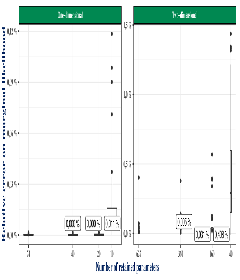
Refer to caption
Figure 9: Distribution of the discrepancies induced by the proposed rank reduction method, depending on the number of retained eigenvectors during the selection of the smoothing parameter, in the one-dimensional and two-dimensional case.

Figure 9 represents the impact of rank reduction on the smoothing results as a function of the number of retained components. In the one-dimensional case, reducing the number of retained eigenvectors from 74 to 10 has only a marginal impact on the results obtained. However, as shown in Figure 10, it reduces the computation time by a factor of 3. In the two-dimensional case, reducing the number of components to 160 reduces the computation time by a factor close to 10, with imperceptible differences in the obtained results. The proposed rank reduction method, in combination with the performance iteration approach, thus allows, in the two-dimensional case, by considering only 160 components, to reduce the computation time by a factor of 40 at the cost of an average error of 0.03%, which exceeds 0.5% in only one of the 100 simulated datasets considered. This solution offers significant operational advantages, especially for applications mentioned in Section 6.1 where computation times can be much more significant than in the analysis presented here.
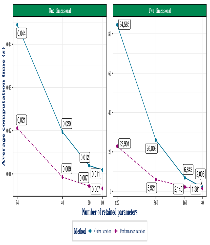
Refer to caption
Figure 10: Distribution of computation time for the proposed rank reduction method, depending on the number of retained eigenvectors during the selection of the smoothing parameter, in the one-dimensional and two-dimensional case.

7 How to extrapolate the smoothing?

7.1 Defining the (unconstrained) extrapolation of the smoothing

Let 𝐲^^𝐲\hat{\mathbf{y}} be the result of Whittaker-Henderson smoothing for an observation vector 𝐲𝐲\mathbf{y}, which corresponds in the one-dimensional case to an explanatory variable vector 𝐱𝐱\mathbf{x} or in the two-dimensional case to a combination of explanatory variables 𝐱𝐱\mathbf{x} and 𝐳𝐳\mathbf{z}. Suppose we have an observation vector 𝐱+subscript𝐱\mathbf{x}_{+} or combinations of vectors 𝐱+subscript𝐱\mathbf{x}_{+} and 𝐳+subscript𝐳\mathbf{z}_{+} for which we want to make predictions using the model. Since Whittaker-Henderson smoothing applies only to evenly spaced observations, without loss of generality, let 𝐱+subscript𝐱\mathbf{x}_{+} and 𝐳+subscript𝐳\mathbf{z}_{+} be sequences of consecutive integers such that 𝐱𝐱+𝐱subscript𝐱\mathbf{x}\subset\mathbf{x}_{+} and 𝐳𝐳+𝐳subscript𝐳\mathbf{z}\subset\mathbf{z}_{+}. In the one-dimensional case, let n+subscript𝑛n_{+} be the length of 𝐱+subscript𝐱\mathbf{x}_{+}, and in the two-dimensional case, let nx+subscript𝑛limit-from𝑥n_{x+} and nz+subscript𝑛limit-from𝑧n_{z+} be the respective lengths of 𝐱+subscript𝐱\mathbf{x}_{+} and 𝐳+subscript𝐳\mathbf{z}_{+}, with n+=nx+×nz+subscript𝑛subscript𝑛limit-from𝑥subscript𝑛limit-from𝑧n_{+}=n_{x+}\times n_{z+}. Let Cxsubscript𝐶𝑥C_{x} (resp. Czsubscript𝐶𝑧C_{z}) be a matrix of size nx×nx+subscript𝑛𝑥subscript𝑛limit-from𝑥n_{x}\times n_{x+} (resp. nz×nz+subscript𝑛𝑧subscript𝑛limit-from𝑧n_{z}\times n_{z+}) defined as Cj=(0nj,minjminj+|Inj,nj|0nj,maxj+maxj)subscript𝐶𝑗subscript0subscript𝑛𝑗𝑗subscript𝑗subscript𝐼subscript𝑛𝑗subscript𝑛𝑗subscript0subscript𝑛𝑗subscript𝑗𝑗C_{j}=(0_{n_{j},\min j-\min j_{+}}|I_{n_{j},n_{j}}|0_{n_{j},\max j_{+}-\max j}) for j{x,z}𝑗𝑥𝑧j\in\{x,z\}, and let us note:

C={Cxin the one-dimensional caseCzCxin the two-dimensional case𝐶casessubscript𝐶𝑥in the one-dimensional casetensor-productsubscript𝐶𝑧subscript𝐶𝑥in the two-dimensional caseC=\begin{cases}C_{x}&\text{in the one-dimensional case}\\ C_{z}\otimes C_{x}&\text{in the two-dimensional case}\end{cases}

The matrix C𝐶C of size n×n+𝑛subscript𝑛n\times n_{+} defined in this way has the following properties:

  • \bullet

    For any vector 𝐲+subscript𝐲\mathbf{y}_{+} of size n+subscript𝑛n_{+}, C𝐲+𝐶subscript𝐲C\mathbf{y}_{+} is a vector of size n𝑛n containing only the n𝑛n values of 𝐲+subscript𝐲\mathbf{y}_{+} matching the positions of the observations in the initial smoothing,

  • \bullet

    CT𝐲superscript𝐶𝑇𝐲C^{T}\mathbf{y} is a vector of size n+subscript𝑛n_{+} containing the values of 𝐲𝐲\mathbf{y} at the positions corresponding to the initial observations and zeros elsewhere,

  • \bullet

    CCT=In𝐶superscript𝐶𝑇subscript𝐼𝑛CC^{T}=I_{n}.

The extrapolation of Whittaker-Henderson smoothing can now be defined as finding the solution 𝐲^+subscript^𝐲\hat{\mathbf{y}}_{+} to the extended optimization problem:

𝐲^+=argmin𝜽+{(𝐲+𝜽+)TW+(𝐲+𝜽+)+𝜽+TP+𝜽+}subscript^𝐲subscript𝜽argminsuperscriptsubscript𝐲subscript𝜽𝑇subscript𝑊subscript𝐲subscript𝜽superscriptsubscript𝜽𝑇subscript𝑃subscript𝜽\hypertarget{eq-extra1}{}{\hat{\mathbf{y}}_{+}=\underset{\boldsymbol{\theta}_{+}}{\text{argmin}}\left\{(\mathbf{y}_{+}-\boldsymbol{\theta}_{+})^{T}W_{+}(\mathbf{y}_{+}-\boldsymbol{\theta}_{+})+\boldsymbol{\theta}_{+}^{T}P_{+}\boldsymbol{\theta}_{+}\right\}} (22)

where 𝐲+=CT𝐲subscript𝐲superscript𝐶𝑇𝐲\mathbf{y}_{+}=C^{T}\mathbf{y}, W+=CTWCsubscript𝑊superscript𝐶𝑇𝑊𝐶W_{+}=C^{T}WC, and

P+={λDn+,qTDn+,qin the one-dimensional caseλxIz+Dnx+,qxTDnx+,qx+λzDnz+,qzTDnz+,qzIx+in the two-dimensional casesubscript𝑃cases𝜆superscriptsubscript𝐷subscript𝑛𝑞𝑇subscript𝐷subscript𝑛𝑞in the one-dimensional casetensor-productsubscript𝜆𝑥subscript𝐼limit-from𝑧superscriptsubscript𝐷subscript𝑛limit-from𝑥subscript𝑞𝑥𝑇subscript𝐷subscript𝑛limit-from𝑥subscript𝑞𝑥tensor-productsubscript𝜆𝑧superscriptsubscript𝐷subscript𝑛limit-from𝑧subscript𝑞𝑧𝑇subscript𝐷subscript𝑛limit-from𝑧subscript𝑞𝑧subscript𝐼limit-from𝑥in the two-dimensional caseP_{+}=\begin{cases}\lambda D_{n_{+},q}^{T}D_{n_{+},q}&\text{in the one-dimensional case}\\ \lambda_{x}I_{z+}\otimes D_{n_{x+},q_{x}}^{T}D_{n_{x+},q_{x}}+\lambda_{z}D_{n_{z+},q_{z}}^{T}D_{n_{z+},q_{z}}\otimes I_{x+}&\text{in the two-dimensional case}\end{cases}

In this last expression, λ𝜆\lambda, λxsubscript𝜆𝑥\lambda_{x} and λzsubscript𝜆𝑧\lambda_{z} are the parameters chosen for the smoothing. Similar to the initial smoothing, Equation 22 involves a fidelity criterion and a smoothness criterion. It should be noted that:

(𝐲+𝜽+)TW+(𝐲+𝜽+)=(CT𝐲𝜽+)TCTWC(CT𝐲𝜽+)=(𝐲𝜽)TW(𝐲𝜽)superscriptsubscript𝐲subscript𝜽𝑇subscript𝑊subscript𝐲subscript𝜽superscriptsuperscript𝐶𝑇𝐲subscript𝜽𝑇superscript𝐶𝑇𝑊𝐶superscript𝐶𝑇𝐲subscript𝜽superscript𝐲𝜽𝑇𝑊𝐲𝜽(\mathbf{y}_{+}-\boldsymbol{\theta}_{+})^{T}W_{+}(\mathbf{y}_{+}-\boldsymbol{\theta}_{+})=(C^{T}\mathbf{y}-\boldsymbol{\theta}_{+})^{T}C^{T}WC(C^{T}\mathbf{y}-\boldsymbol{\theta}_{+})=(\mathbf{y}-\boldsymbol{\theta})^{T}W(\mathbf{y}-\boldsymbol{\theta})

hence the fidelity criterion remains unchanged compared to the initial estimation problem. This is consistent with the fact that extrapolation does not involve any additional data. The smoothness criterion, however, applies to all elements of the vector 𝜽+subscript𝜽\boldsymbol{\theta}_{+}, whether initially present or not.

7.2 Unconstrained solution for the one-dimensional case

The solution to the extended optimization problem of Equation 22 is readily obtained by taking the derivatives in 𝜽+subscript𝜽\boldsymbol{\theta}_{+} and setting them to 0, as in Section 1.5. This yields the solution:

𝐲^+=(W++P+)1W+𝐲+where𝐲+=CT𝐲andW+=CTWCformulae-sequencesubscript^𝐲superscriptsubscript𝑊subscript𝑃1subscript𝑊subscript𝐲whereformulae-sequencesubscript𝐲superscript𝐶𝑇𝐲andsubscript𝑊superscript𝐶𝑇𝑊𝐶\hypertarget{eq-extra2}{}{\hat{\mathbf{y}}_{+}=(W_{+}+P_{+})^{-1}W_{+}\mathbf{y}_{+}\quad\text{where}\quad\mathbf{y}_{+}=C^{T}\mathbf{y}\quad\text{and}\quad W_{+}=C^{T}WC} (23)

Let us further assume that 𝐲+|𝜽+𝒩(𝜽+,W+)similar-toconditionalsubscript𝐲subscript𝜽𝒩subscript𝜽superscriptsubscript𝑊\mathbf{y}_{+}|\boldsymbol{\theta_{+}}\sim\mathcal{N}(\boldsymbol{\theta}_{+},W_{+}^{-}) where 𝜽+𝒩(0,P+)similar-tosubscript𝜽𝒩0superscriptsubscript𝑃\boldsymbol{\theta}_{+}\sim\mathcal{N}(0,P_{+}^{-}) and procede as in Section 2 to obtain the following credible intervals:

𝔼(𝐲+)|𝐲+[(W++P+)1W+𝐲+±Φ1(1α2)diag{(W++P+)1}]conditional𝔼subscript𝐲subscript𝐲delimited-[]plus-or-minussuperscriptsubscript𝑊subscript𝑃1subscript𝑊subscript𝐲superscriptΦ11𝛼2diagsuperscriptsubscript𝑊subscript𝑃1\hypertarget{eq-IC-extra}{}{\mathbb{E}(\mathbf{y}_{+})|\mathbf{y}_{+}\in\left[(W_{+}+P_{+})^{-1}W_{+}\mathbf{y}_{+}\pm\Phi^{-1}\left(1-\frac{\alpha}{2}\right)\sqrt{\textbf{diag}\left\{(W_{+}+P_{+})^{-1}\right\}}\right]} (24)

To get a better understanding about how the variance-covariance matrix Ψ+=(W++P+)1subscriptΨsuperscriptsubscript𝑊subscript𝑃1\Psi_{+}=(W_{+}+P_{+})^{-1} for the unconstrained extrapolation problem of Equation 22 is related to the variance-covariance matrix Ψ=(W+Pλ)1Ψsuperscript𝑊subscript𝑃𝜆1\Psi=(W+P_{\lambda})^{-1} of the original smoothing problem, let us introduce:

C¯j=[Iminjminj+,minjminj+0minjminj+,nj0minjminj+,maxj+maxj0maxj+maxj,minjminj+0maxj+maxj,njImaxj+maxj,maxj+maxj]forj{x,z},formulae-sequencesubscript¯𝐶𝑗matrixsubscript𝐼𝑗subscript𝑗𝑗subscript𝑗subscript0𝑗subscript𝑗subscript𝑛𝑗subscript0𝑗subscript𝑗subscript𝑗𝑗subscript0subscript𝑗𝑗𝑗subscript𝑗subscript0subscript𝑗𝑗subscript𝑛𝑗subscript𝐼subscript𝑗𝑗subscript𝑗𝑗for𝑗𝑥𝑧\overline{C}_{j}=\begin{bmatrix}I_{\min j-\min j_{+},\min j-\min j_{+}}&0_{\min j-\min j_{+},n_{j}}&0_{\min j-\min j_{+},\max j_{+}-\max j}\\ 0_{\max j_{+}-\max j,\min j-\min j_{+}}&0_{\max j_{+}-\max j,n_{j}}&I_{\max j_{+}-\max j,\max j_{+}-\max j}\end{bmatrix}\quad\text{for}\quad j\in\{x,z\},
C¯={C¯xin the one-dimensional caseC¯zC¯xin the two-dimensional caseandQ=[CC¯].formulae-sequence¯𝐶casessubscript¯𝐶𝑥in the one-dimensional casetensor-productsubscript¯𝐶𝑧subscript¯𝐶𝑥in the two-dimensional caseand𝑄matrix𝐶¯𝐶\quad\overline{C}=\begin{cases}\overline{C}_{x}&\text{in the one-dimensional case}\\ \overline{C}_{z}\otimes\overline{C}_{x}&\text{in the two-dimensional case}\end{cases}\quad\text{and}\quad Q=\begin{bmatrix}C\\ \overline{C}\end{bmatrix}.

With this definition, Q𝑄Q is a permutation matrix of size n+×n+subscript𝑛subscript𝑛n_{+}\times n_{+} which select the rows whose indices correspond to those of the initial observation positions in the extended observation vector and put them first. It also verifies Q1=QT=Qsuperscript𝑄1superscript𝑄𝑇𝑄Q^{-1}=Q^{T}=Q.

In the unidimensional case, the extended difference matrix Dn+,qsubscript𝐷subscript𝑛𝑞D_{n_{+},q} takes the form:

Dn+,q=[D2D100Dn,q00D1+D2+]=Q[Dn,q00D1D20D1+0D2+]Q=Q[Dn,q0D1D2]Qsubscript𝐷subscript𝑛𝑞matrixsubscript𝐷limit-from2subscript𝐷limit-from100subscript𝐷𝑛𝑞00subscript𝐷limit-from1subscript𝐷limit-from2𝑄matrixsubscript𝐷𝑛𝑞00subscript𝐷limit-from1subscript𝐷limit-from20subscript𝐷limit-from10subscript𝐷limit-from2𝑄𝑄matrixsubscript𝐷𝑛𝑞0subscript𝐷1subscript𝐷2𝑄D_{n_{+},q}=\begin{bmatrix}D_{2-}&D_{1-}&0\\ 0&D_{n,q}&0\\ 0&D_{1+}&D_{2+}\\ \end{bmatrix}=Q\begin{bmatrix}D_{n,q}&0&0\\ D_{1-}&D_{2-}&0\\ D_{1+}&0&D_{2+}\\ \end{bmatrix}Q=Q\begin{bmatrix}D_{n,q}&0\\ D_{1}&D_{2}\\ \end{bmatrix}Q
whereD1=[D1D1+]andD2=[D200D2+]formulae-sequencewheresubscript𝐷1matrixsubscript𝐷limit-from1subscript𝐷limit-from1andsubscript𝐷2matrixsubscript𝐷limit-from200subscript𝐷limit-from2\quad\text{where}\quad D_{1}=\begin{bmatrix}D_{1-}\\ D_{1+}\\ \end{bmatrix}\quad\text{and}\quad D_{2}=\begin{bmatrix}D_{2-}&0\\ 0&D_{2+}\\ \end{bmatrix}

Detailed expressions of matrices D1+subscript𝐷limit-from1D_{1+} and D2+subscript𝐷limit-from2D_{2+} for the most common values of q𝑞q may be found in Carballo et al. (2021) where they are simply noted D1subscript𝐷1D_{1} and D2subscript𝐷2D_{2}. To cover extrapolation on both sides of the initial observation vector, matrices D1subscript𝐷limit-from1D_{1-} and D2subscript𝐷limit-from2D_{2-} were introduced. Those may be simply obtained by taking the transpose of adequate size D1subscript𝐷1D_{1} and D2subscript𝐷2D_{2} matrices found in Carballo et al. (2021). The extended weight and penalization matrices thus take the form:

W+=Q[W000]QandP+=Dn+,qTDn+,q=λQ[Pλ+P+11P+12P+21P+22]Qformulae-sequencesubscript𝑊𝑄matrix𝑊000𝑄andsubscript𝑃superscriptsubscript𝐷subscript𝑛𝑞𝑇subscript𝐷subscript𝑛𝑞𝜆𝑄matrixsubscript𝑃𝜆superscriptsubscript𝑃11superscriptsubscript𝑃12superscriptsubscript𝑃21superscriptsubscript𝑃22𝑄\hypertarget{eq-expr-P}{}{W_{+}=Q\begin{bmatrix}W&0\\ 0&0\\ \end{bmatrix}Q\quad\text{and}\quad P_{+}=D_{n_{+},q}^{T}D_{n_{+},q}=\lambda Q\begin{bmatrix}P_{\lambda}+P_{+}^{11}&P_{+}^{12}\\ P_{+}^{21}&P_{+}^{22}\\ \end{bmatrix}Q} (25)

where P+11=λD1TD1superscriptsubscript𝑃11𝜆superscriptsubscript𝐷1𝑇subscript𝐷1P_{+}^{11}=\lambda D_{1}^{T}D_{1}, P+12=λD1TD2superscriptsubscript𝑃12𝜆superscriptsubscript𝐷1𝑇subscript𝐷2P_{+}^{12}=\lambda D_{1}^{T}D_{2}, P+21=λD2TD1superscriptsubscript𝑃21𝜆superscriptsubscript𝐷2𝑇subscript𝐷1P_{+}^{21}=\lambda D_{2}^{T}D_{1} and P+22=λD2TD2superscriptsubscript𝑃22𝜆superscriptsubscript𝐷2𝑇subscript𝐷2P_{+}^{22}=\lambda D_{2}^{T}D_{2}.

Applying the formulas for the inversion of a symmetric matrix partitioned with 2×2222\times 2 blocks to Q(W++P+)Q𝑄subscript𝑊subscript𝑃𝑄Q(W_{+}+P_{+})Q, we obtain a more detailed expression for Ψ+subscriptΨ\Psi_{+}:

Ψ+=Q[Ψ+11Ψ+11P+12(P+22)1(P+22)1P+21Ψ+11(P+22)1+(P+22)1P+21Ψ+11P+12(P+22)1]Q.subscriptΨ𝑄matrixsuperscriptsubscriptΨ11superscriptsubscriptΨ11superscriptsubscript𝑃12superscriptsuperscriptsubscript𝑃221superscriptsuperscriptsubscript𝑃221superscriptsubscript𝑃21superscriptsubscriptΨ11superscriptsuperscriptsubscript𝑃221superscriptsuperscriptsubscript𝑃221superscriptsubscript𝑃21superscriptsubscriptΨ11superscriptsubscript𝑃12superscriptsuperscriptsubscript𝑃221𝑄\hypertarget{eq-Psi-extra}{}{\Psi_{+}=Q\begin{bmatrix}\Psi_{+}^{11}&-\Psi_{+}^{11}P_{+}^{12}(P_{+}^{22})^{-1}\\ -(P_{+}^{22})^{-1}P_{+}^{21}\Psi_{+}^{11}&(P_{+}^{22})^{-1}+(P_{+}^{22})^{-1}P_{+}^{21}\Psi_{+}^{11}P_{+}^{12}(P_{+}^{22})^{-1}\end{bmatrix}Q.} (26)

where Ψ+11=[W+Pλ+P+11P+12(P+22)1P+21]1superscriptsubscriptΨ11superscriptdelimited-[]𝑊subscript𝑃𝜆superscriptsubscript𝑃11superscriptsubscript𝑃12superscriptsuperscriptsubscript𝑃221superscriptsubscript𝑃211\Psi_{+}^{11}=[W+P_{\lambda}+P_{+}^{11}-P_{+}^{12}(P_{+}^{22})^{-1}P_{+}^{21}]^{-1}.

Let us denote by initial positions coefficients the subvector C𝐲^+𝐶subscript^𝐲C\hat{\mathbf{y}}_{+} that correspond to the coefficients at the position of the initial observations in 𝐲^+subscript^𝐲\hat{\mathbf{y}}_{+} and by new positions coefficients the remaining coefficients C¯𝐲^+¯𝐶subscript^𝐲\overline{C}\hat{\mathbf{y}}_{+}. The initial positions coefficients may be recovered as C𝐲^+=CΨ+CTW+y+=Ψ+11Wy𝐶subscript^𝐲𝐶subscriptΨsuperscript𝐶𝑇subscript𝑊subscript𝑦superscriptsubscriptΨ11𝑊𝑦C\hat{\mathbf{y}}_{+}=C\Psi_{+}C^{T}W_{+}y_{+}=\Psi_{+}^{11}Wy. This does not simplify to ΨWy=𝐲^Ψ𝑊𝑦^𝐲\Psi Wy=\hat{\mathbf{y}} for all weighted observation vectors Wy𝑊𝑦Wy unless Ψ+11=ΨsuperscriptsubscriptΨ11Ψ\Psi_{+}^{11}=\Psi. Indeed, the initial positions coefficients are chosen to optimize the overall smoothness of the extrapolated coefficient vectors and note just the smoothness of C𝐲^+𝐶subscript^𝐲C\hat{\mathbf{y}}_{+}. Besides, the expression of Ψ+22superscriptsubscriptΨ22\Psi_{+}^{22}, it contains two terms: an innovation error (P+22)1superscriptsuperscriptsubscript𝑃221(P_{+}^{22})^{-1} associated with the prior on the new positions coefficients while (P+22)1P+21Ψ+11P+12(P+22)1superscriptsuperscriptsubscript𝑃221superscriptsubscript𝑃21superscriptsubscriptΨ11superscriptsubscript𝑃12superscriptsuperscriptsubscript𝑃221(P_{+}^{22})^{-1}P_{+}^{21}\Psi_{+}^{11}P_{+}^{12}(P_{+}^{22})^{-1} represents an additional uncertainty on the new positions coefficients caused by the uncertainty on the initial positions coefficients.

In the one-dimensional case, D2subscript𝐷2D_{2} is a block-diagonal matrix of triangular matrices with non-zero diagonal elements and is thus non-singular. Hence P+11P+12(P+22)1P+21=D1TD1D1TD2(D2TD2)1D2TD1=0superscriptsubscript𝑃11superscriptsubscript𝑃12superscriptsuperscriptsubscript𝑃221superscriptsubscript𝑃21superscriptsubscript𝐷1𝑇subscript𝐷1superscriptsubscript𝐷1𝑇subscript𝐷2superscriptsuperscriptsubscript𝐷2𝑇subscript𝐷21𝐷superscript2𝑇subscript𝐷10P_{+}^{11}-P_{+}^{12}(P_{+}^{22})^{-1}P_{+}^{21}=D_{1}^{T}D_{1}-D_{1}^{T}D_{2}(D_{2}^{T}D_{2})^{-1}D2^{T}D_{1}=0 which means that Ψ+11=(W+Pλ)1=ΨsuperscriptsubscriptΨ11superscript𝑊subscript𝑃𝜆1Ψ\Psi_{+}^{11}=(W+P_{\lambda})^{-1}=\Psi and C𝐲^+=𝐲^𝐶subscript^𝐲^𝐲C\hat{\mathbf{y}}_{+}=\hat{\mathbf{y}}. Therefore, in the one-dimensional case, the solution given by Equation 22 preserves the values from the original fit. As shown by Carballo et al. (2021), it is indeed always possible in the case of penalizations based on difference matrices to pick the new positions coefficients so that the smoothness criterion does not increase or in other words to find a perfectly smooth extrapolation for the fit. Figure 11 shows the extrapolation associated with the Whittaker-Henderson smoothing applied to the data use to produce Figure 1.
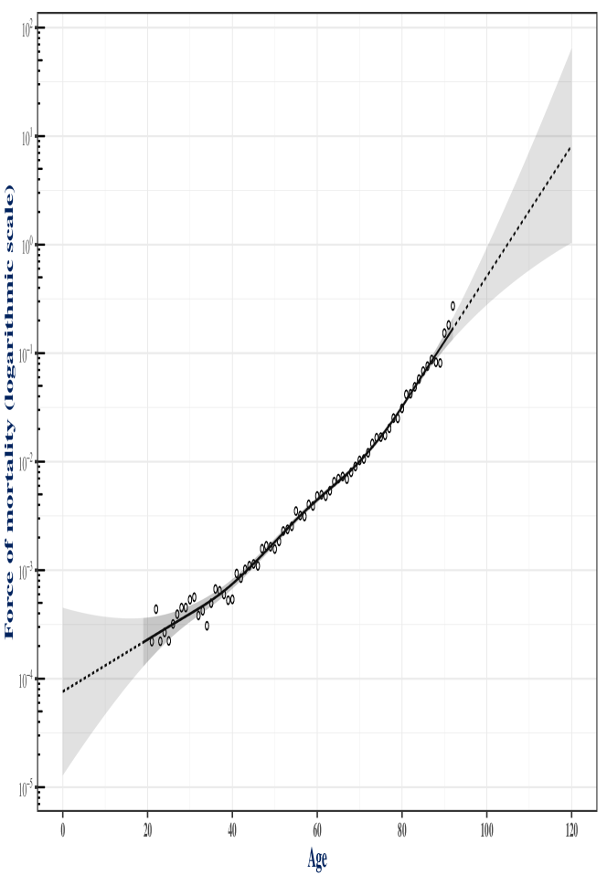
Refer to caption
Figure 11: Extrapolation of Whittaker-Henderson smoothing in the one-dimensional case. The smoother extrapolation is achieved, on both sides of the smoothing, using a polynomial of degree q - 1 (in this case a straight line as q = 2).

7.3 Constrained solution for the two-dimensional case

In the two-dimensional case, while the extended penalization matrix P+subscript𝑃P_{+} still takes the form of Equation 25, expressions of P+11superscriptsubscript𝑃11P_{+}^{11}, P+12superscriptsubscript𝑃12P_{+}^{12}, P+21superscriptsubscript𝑃21P_{+}^{21} and P+22superscriptsubscript𝑃22P_{+}^{22} are more complex. In particular, P+11P+12(P+22)1P+210superscriptsubscript𝑃11superscriptsubscript𝑃12superscriptsuperscriptsubscript𝑃221superscriptsubscript𝑃210P_{+}^{11}-P_{+}^{12}(P_{+}^{22})^{-1}P_{+}^{21}\neq 0 which implies that Ψ+11ΨsuperscriptsubscriptΨ11Ψ\Psi_{+}^{11}\neq\Psi and C𝐲^+𝐲^𝐶subscript^𝐲^𝐲C\hat{\mathbf{y}}_{+}\neq\hat{\mathbf{y}}. Solving Equation 23 thus leads to a change in the value of the initial positions coefficients compared to the coefficients obtained during the initial smoothing as shown by Carballo, Durban, and Lee (2021). Indeed, the smoothness criterion includes penalizations on both rows and columns and it is no longer possible, as in the one-dimensional case, to extrapolate the fit without increasing that criterion. As the smoothness criterion carries more weight in the extrapolation problem compared to the original problem, the optimal solution to the extended optimization problem will compromise on the fidelity to the initial observations in order to improve the overall smoothness.

To obtain an estimator 𝐲^+subscriptsuperscript^𝐲\hat{\mathbf{y}}^{\ast}_{+} that minimizes the penalized regression problem under the constraint of preserving the initial coefficients, i.e. C𝐲^+=𝐲^𝐶subscriptsuperscript^𝐲^𝐲C\hat{\mathbf{y}}^{\ast}_{+}=\hat{\mathbf{y}}, we follow the approach proposed by Carballo, Durban, and Lee (2021) and introduce the Lagrange multiplier 𝝎𝝎\boldsymbol{\omega}. The associated constrained extended optimization problem is now written as:

(𝐲^+,𝝎^)=argmin𝜽+,𝝎{(𝐲+𝜽+)TW+(𝐲+𝜽+)+𝜽+TP+𝜽++2𝝎T(C𝜽+𝐲^)}.superscriptsubscript^𝐲^𝝎superscriptsubscript𝜽𝝎argminsuperscriptsubscript𝐲superscriptsubscript𝜽𝑇subscript𝑊subscript𝐲superscriptsubscript𝜽superscriptsubscript𝜽absent𝑇subscript𝑃superscriptsubscript𝜽2superscript𝝎𝑇𝐶superscriptsubscript𝜽^𝐲\hypertarget{eq-optim-lagrange}{}{(\hat{\mathbf{y}}_{+}^{\ast},\hat{\boldsymbol{\omega}})=\underset{\boldsymbol{\theta}_{+}^{\ast},\boldsymbol{\omega}}{\text{argmin}}\left\{(\mathbf{y}_{+}-\boldsymbol{\theta}_{+}^{\ast})^{T}W_{+}(\mathbf{y}_{+}-\boldsymbol{\theta}_{+}^{\ast})+\boldsymbol{\theta}_{+}^{\ast T}P_{+}\boldsymbol{\theta}_{+}^{\ast}+2\boldsymbol{\omega}^{T}(C\boldsymbol{\theta}_{+}^{\ast}-\hat{\mathbf{y}})\right\}.} (27)

Taking the partial derivatives of Equation 27 with respect to 𝜽+superscriptsubscript𝜽\boldsymbol{\theta}_{+}^{\ast} and 𝝎𝝎\boldsymbol{\omega} gives:

𝜽+{(𝐲+𝜽+)TW+(𝐲+𝜽+)+𝜽+TP+𝜽++2𝝎T(C𝜽+𝐲^)}superscriptsubscript𝜽superscriptsubscript𝐲superscriptsubscript𝜽𝑇subscript𝑊subscript𝐲superscriptsubscript𝜽superscriptsubscript𝜽absent𝑇subscript𝑃superscriptsubscript𝜽2superscript𝝎𝑇𝐶superscriptsubscript𝜽^𝐲\displaystyle\frac{\partial}{\partial\boldsymbol{\theta}_{+}^{\ast}}\left\{(\mathbf{y}_{+}-\boldsymbol{\theta}_{+}^{\ast})^{T}W_{+}(\mathbf{y}_{+}-\boldsymbol{\theta}_{+}^{\ast})+\boldsymbol{\theta}_{+}^{\ast T}P_{+}\boldsymbol{\theta}_{+}^{\ast}+2\boldsymbol{\omega}^{T}(C\boldsymbol{\theta}_{+}^{\ast}-\hat{\mathbf{y}})\right\} =2W+(𝐲+𝜽+)+2P+𝜽++2𝝎TCabsent2subscript𝑊subscript𝐲superscriptsubscript𝜽2subscript𝑃superscriptsubscript𝜽2superscript𝝎𝑇𝐶\displaystyle=-2W_{+}(\mathbf{y}_{+}-\boldsymbol{\theta}_{+}^{\ast})+2P_{+}\boldsymbol{\theta}_{+}^{\ast}+2\boldsymbol{\omega}^{T}C
𝝎{(𝐲+𝜽+)TW+(𝐲+𝜽+)+𝜽+TP+𝜽++2𝝎T(C𝜽+𝐲^)}𝝎superscriptsubscript𝐲superscriptsubscript𝜽𝑇subscript𝑊subscript𝐲superscriptsubscript𝜽superscriptsubscript𝜽absent𝑇subscript𝑃superscriptsubscript𝜽2superscript𝝎𝑇𝐶superscriptsubscript𝜽^𝐲\displaystyle\frac{\partial}{\partial\boldsymbol{\boldsymbol{\omega}}}\left\{(\mathbf{y}_{+}-\boldsymbol{\theta}_{+}^{\ast})^{T}W_{+}(\mathbf{y}_{+}-\boldsymbol{\theta}_{+}^{\ast})+\boldsymbol{\theta}_{+}^{\ast T}P_{+}\boldsymbol{\theta}_{+}^{\ast}+2\boldsymbol{\omega}^{T}(C\boldsymbol{\theta}_{+}^{\ast}-\hat{\mathbf{y}})\right\} =2(C𝜽+𝐲^)absent2𝐶superscriptsubscript𝜽^𝐲\displaystyle=2(C\boldsymbol{\theta}_{+}^{\ast}-\hat{\mathbf{y}})

Setting these derivatives to zero yields the linear system:

[W++P+CTC0][𝐲^+𝝎^]=[W+𝐲+𝐲^]matrixsubscript𝑊subscript𝑃superscript𝐶𝑇𝐶0matrixsubscriptsuperscript^𝐲^𝝎matrixsubscript𝑊subscript𝐲^𝐲\begin{bmatrix}W_{+}+P_{+}&C^{T}\\ C&0\end{bmatrix}\begin{bmatrix}\hat{\mathbf{y}}^{\ast}_{+}\\ \hat{\boldsymbol{\omega}}\end{bmatrix}=\begin{bmatrix}W_{+}\mathbf{y}_{+}\\ \hat{\mathbf{y}}\end{bmatrix}

The solution for 𝐲^+subscriptsuperscript^𝐲\hat{\mathbf{y}}^{\ast}_{+} can be derived using formulas for the inversion of a symmetric partitioned matrix with 2×2222\times 2 blocks:

𝐲^+=subscriptsuperscript^𝐲absent\displaystyle\hat{\mathbf{y}}^{\ast}_{+}= (W++P+)1{ICT[C(W++P+)1CT]1C(W++P+)1}W+𝐲+superscriptsubscript𝑊subscript𝑃1𝐼superscript𝐶𝑇superscriptdelimited-[]𝐶superscriptsubscript𝑊subscript𝑃1superscript𝐶𝑇1𝐶superscriptsubscript𝑊subscript𝑃1subscript𝑊subscript𝐲\displaystyle(W_{+}+P_{+})^{-1}\left\{I-C^{T}[C(W_{+}+P_{+})^{-1}C^{T}]^{-1}C(W_{+}+P_{+})^{-1}\right\}W_{+}\mathbf{y}_{+}
+(W++P+)1CT[C(W++P+)1CT]1𝐲^superscriptsubscript𝑊subscript𝑃1superscript𝐶𝑇superscriptdelimited-[]𝐶superscriptsubscript𝑊subscript𝑃1superscript𝐶𝑇1^𝐲\displaystyle+(W_{+}+P_{+})^{-1}C^{T}[C(W_{+}+P_{+})^{-1}C^{T}]^{-1}\hat{\mathbf{y}}

Since W+=CTWCsubscript𝑊superscript𝐶𝑇𝑊𝐶W_{+}=C^{T}WC, the first term is actually zero, and this expression simplifies to:

𝐲^+=(W++P+)1CT[C(W++P+)1CT]1𝐲^=Q[IΨ21(Ψ11)1]𝐲^=Q[I(P+22)1P+21]𝐲^subscriptsuperscript^𝐲superscriptsubscript𝑊subscript𝑃1superscript𝐶𝑇superscriptdelimited-[]𝐶superscriptsubscript𝑊subscript𝑃1superscript𝐶𝑇1^𝐲𝑄matrix𝐼superscriptΨ21superscriptsuperscriptΨ111^𝐲𝑄matrix𝐼superscriptsuperscriptsubscript𝑃221superscriptsubscript𝑃21^𝐲\hypertarget{eq-extra3}{}{\hat{\mathbf{y}}^{\ast}_{+}=(W_{+}+P_{+})^{-1}C^{T}[C(W_{+}+P_{+})^{-1}C^{T}]^{-1}\hat{\mathbf{y}}=Q\begin{bmatrix}I\\ \Psi^{21}(\Psi^{11})^{-1}\end{bmatrix}\hat{\mathbf{y}}=Q\begin{bmatrix}I\\ -(P_{+}^{22})^{-1}P_{+}^{21}\end{bmatrix}\hat{\mathbf{y}}} (28)

which is a linear transformation of 𝐲^^𝐲\hat{\mathbf{y}}. Defining A+=Q[I(P+22)1P+21]superscriptsubscript𝐴𝑄matrix𝐼superscriptsuperscriptsubscript𝑃221superscriptsubscript𝑃21A_{+}^{*}=Q\begin{bmatrix}I\\ -(P_{+}^{22})^{-1}P_{+}^{21}\end{bmatrix}, a natural candidate for the variance-covariance of 𝐲+|𝜽+conditionalsubscriptsuperscript𝐲subscript𝜽\mathbf{y}^{*}_{+}|\boldsymbol{\theta}_{+} is given by:

A+ΨA+T=Q[ΨΨP+12(P+22)1(P+22)1P+21Ψ(P+22)1P+21ΨP+12(P+22)1]Qsuperscriptsubscript𝐴Ψsuperscriptsubscript𝐴absent𝑇𝑄matrixΨΨsuperscriptsubscript𝑃12superscriptsuperscriptsubscript𝑃221superscriptsuperscriptsubscript𝑃221superscriptsubscript𝑃21Ψsuperscriptsuperscriptsubscript𝑃221superscriptsubscript𝑃21Ψsuperscriptsubscript𝑃12superscriptsuperscriptsubscript𝑃221𝑄\hypertarget{eq-Psi-extra2}{}{A_{+}^{*}\Psi A_{+}^{*T}=Q\begin{bmatrix}\Psi&-\Psi P_{+}^{12}(P_{+}^{22})^{-1}\\ -(P_{+}^{22})^{-1}P_{+}^{21}\Psi&(P_{+}^{22})^{-1}P_{+}^{21}\Psi P_{+}^{12}(P_{+}^{22})^{-1}\end{bmatrix}Q} (29)

Equation 29 is very similar to Equation 26 with however two differences. First, every occurence of Ψ+11superscriptsubscriptΨ11\Psi_{+}^{11} is replaced by ΨΨ\Psi. This is consistent with the constraint that the initial positions coefficients are forced to take the value of the coefficients used during the initial smoothing. Second, as the solution to the constrained extended optimization problem of Equation 27 was expressed as a linear transformation of 𝐲^^𝐲\hat{\mathbf{y}}, Equation 29 is missing the innovation error term (P+22)1superscriptsuperscriptsubscript𝑃221(P_{+}^{22})^{-1} associated with the prior on the new positions coefficients. Not including this term would be tantamount to considering that 𝜽+subscript𝜽\boldsymbol{\theta}_{+} has some degree of wigglyness in the region of the initial data but is perfectly smooth everywhere else. Adding the innovation error back, we obtain the following variance-covariance matrix for the constrained optimization problem:

Ψ+=Q[ΨΨP+12(P+22)1(P+22)1P+21Ψ(P+22)1+(P+22)1P+21ΨP+12(P+22)1]QsuperscriptsubscriptΨ𝑄matrixΨΨsuperscriptsubscript𝑃12superscriptsuperscriptsubscript𝑃221superscriptsuperscriptsubscript𝑃221superscriptsubscript𝑃21Ψsuperscriptsuperscriptsubscript𝑃221superscriptsuperscriptsubscript𝑃221superscriptsubscript𝑃21Ψsuperscriptsubscript𝑃12superscriptsuperscriptsubscript𝑃221𝑄\hypertarget{eq-Psi-extra3}{}{\Psi_{+}^{\ast}=Q\begin{bmatrix}\Psi&-\Psi P_{+}^{12}(P_{+}^{22})^{-1}\\ -(P_{+}^{22})^{-1}P_{+}^{21}\Psi&(P_{+}^{22})^{-1}+(P_{+}^{22})^{-1}P_{+}^{21}\Psi P_{+}^{12}(P_{+}^{22})^{-1}\end{bmatrix}Q} (30)

which still verifies

Ψ+W+𝐲+=Ψ+CW𝐲=Q[I(P+22)1P+21]ΨW𝐲=𝐲^+.superscriptsubscriptΨsubscript𝑊subscript𝐲superscriptsubscriptΨ𝐶𝑊𝐲𝑄matrix𝐼superscriptsuperscriptsubscript𝑃221superscriptsubscript𝑃21Ψ𝑊𝐲subscriptsuperscript^𝐲\Psi_{+}^{\ast}W_{+}\mathbf{y}_{+}=\Psi_{+}^{\ast}CW\mathbf{y}=Q\begin{bmatrix}I\\ -(P_{+}^{22})^{-1}P_{+}^{21}\end{bmatrix}\Psi W\mathbf{y}=\hat{\mathbf{y}}^{\ast}_{+}.

The associated credible intervals are readily obtained as:

𝔼(𝐲+)|𝐲+[𝐲^+±Φ1(1α2)diag(Ψ+)]conditional𝔼subscript𝐲subscript𝐲delimited-[]plus-or-minussubscriptsuperscript^𝐲superscriptΦ11𝛼2diagsuperscriptsubscriptΨ\mathbb{E}(\mathbf{y}_{+})|\mathbf{y}_{+}\in\left[\hat{\mathbf{y}}^{\ast}_{+}\pm\Phi^{-1}\left(1-\frac{\alpha}{2}\right)\sqrt{\textbf{diag}(\Psi_{+}^{\ast})}\right]

with probability 1α21𝛼21-\frac{\alpha}{2}, where ΦΦ\Phi denotes the cumulative distribution function of the standard normal distribution.

Figure 12 represents the results of the constrained extrapolation presented in this section, with the associated standard deviation which accounts for the innovation error. It is based on the data used to generate Figure 2. Without the dotted lines marking the boundaries of the initial smoothing region, it would not be possible to tell from those plots where the extrapolation starts, which is precisely the goal of this procedure. Figure 13 represents the ratio between the mortality rates obtained from the unconstrained solution of Equation 23 and the constrained solution of Equation 28. The unconstrained solution shows significant discrepancies both in the initial smoothing region and the extrapolated region compared to the constrained solution. Finally, Figure 14 represents ratios between standard deviation derived using the three presented extrapolation methods. The denominator is the constrained extrapolation method which accounts for the innovation error, which is used as a reference, while the numerator shows the unconstrained method as well as the constrained method which ignores the innovation error. The constrained extrapolation method which includes the innovation error has a higher standard deviation compared to the unconstrained method as it is always either equally or less smooth.
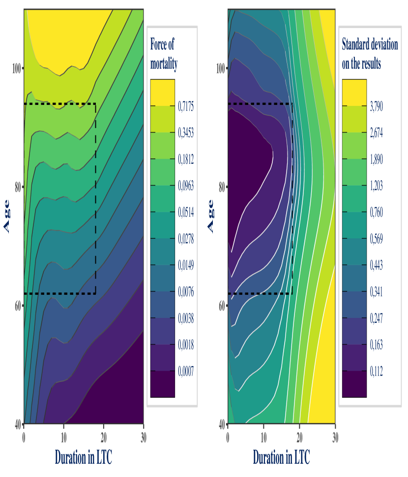
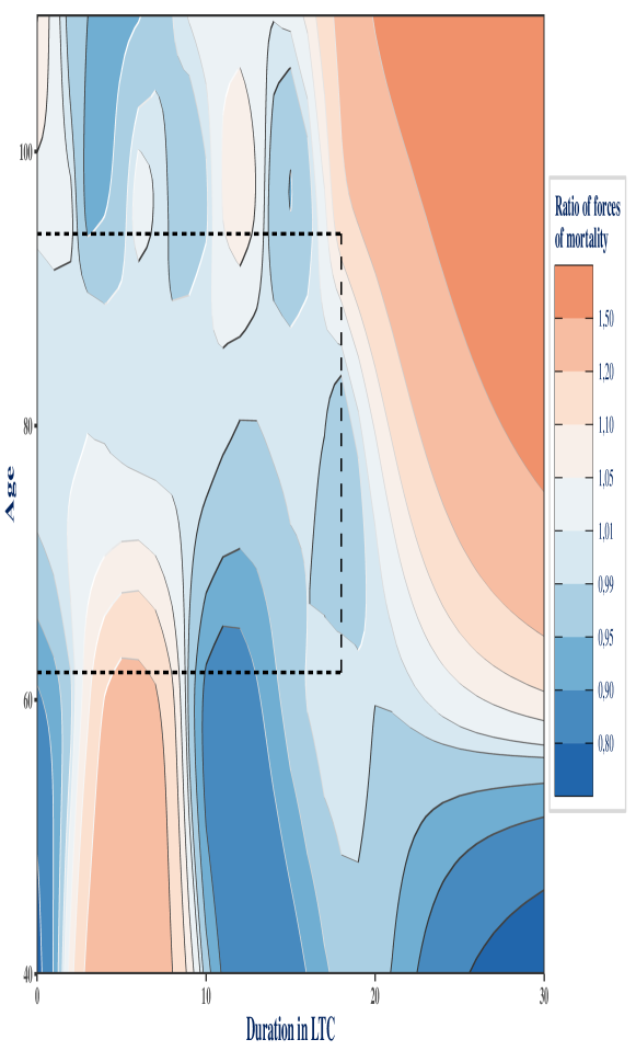
Refer to caption
Figure 12: Constrained extrapolation of Whittaker-Henderson smoothing in the two-dimensional case. The contour lines of mortality rates, and the associated standard deviation, are depicted. The dotted lines delimitate the boundaries boundaries of the initial smoothing region.
Refer to caption
Figure 13: Ratio of mortality rates resulting from the extrapolation of the two-dimensional Whittaker-Henderson smoothing. The numerator corresponds to the unconstrained extrapolation and the denominator represents the constrained extrapolation presented in Figure 12.
Refer to caption
Figure 14: Ratio of standard deviation of log-mortality rates resulting from the extrapolation of the two-dimensional Whittaker-Henderson smoothing. The numerator on the left plot corresponds to the unconstrained extrapolation and on the right plot to the constrained extrapolation that does not account for the innovation error. The denominator represents the constrained extrapolation presented in Figure 12.

8 Discussion

In this paper, we have shown that Whittaker-Henderson smoothing, introduced in 1922, can be naturally interpreted in a Bayesian framework, which allows for the construction of credible intervals for it, provided that the observations are independent and their variances are known and used as weights. By linking it to the framework of duration models, we have demonstrated that in the construction of survival laws from experience, smoothing can be applied to the vector of raw exit rates using the observed number of exits as the weight vector. This is justified by the asymptotic properties of the maximum likelihood estimator of the raw exit rates. We have then established that the use of this asymptotic property comes at the cost of precision loss, especially when the number of observations is limited, and that a more precise iterative version of the smoothing can be proposed by directly solving penalized likelihood equations.

Furthermore, we have introduced an empirical Bayesian approach for selecting the smoothing parameter, based on maximizing a marginal likelihood function. The parameter selection introduces an iterative process that is added to the one generated by solving the penalized likelihood equations for a fixed smoothing parameter. In this case, there are two main possible approaches for parameter selection, depending on the order in which the iterations are nested: the outer iteration and the performance iteration approaches. The latter has significantly lower computation time compared to the former, at the expense of lacking theoretical convergence guarantees, which does not seem to pose a problem in practice. We have also introduced a rank reduction method based on the eigendecomposition of one-dimensional penalty matrices, which accelerates the selection of the smoothing parameter - our study on simulated data showed a 40-fold reduction in computation time - with negligible loss of precision.

Finally, we have addressed the issue of extrapolation of smoothing and shown that it requires solving a new optimization problem. Extrapolation is straightforward in the one-dimensional case. However, in the two-dimensional case constraints needs to be imposed in order to preserve the values of the coefficients obtained during the initial smoothing step.

Whittaker-Henderson smoothing has been used for nearly a century by actuaries, with little change in the approach. In parallel, statistical theory on smoothing methods has undergone numerous developments, particularly in the past 30 years with the emergence of generalized additive models, covered notably by Hastie (2017) and Wood (2006). Our goal in this paper was to bridge the gap between these two perspectives. We also created an R package named WH which implements all the steps mentioned through the paper and should be straightforward to use. The results derived in the paper are directly applicable to other types of smoothing, such as the widely used P-splines smoothing by Eilers and Marx (1996). Compared to Whittaker-Henderson smoothing, P-splines naturally consider fewer parameters than observations, removing the need for the method introduced in Section 6.

While Whittaker-Henderson smoothing is applicable to both the one-dimensional and two-dimensional case, it does have limitations. Firstly, it requires regularly spaced observations. This aligns well with the format of life insurance pricing and reserving assumptions, which traditionally include age and duration spent in certain states that trigger indemnization. However, this can be a limit when the exits are not evenly distributed. For example, in the case of disability and long-term care risks, most exits occur in the first few months following entry into the state. In such situations, using a spline basis that is arranged to prioritize areas with more observations, as proposed by Wood (2017), could yield better results. Lastly, Whittaker-Henderson smoothing does not allow for the incorporation of additional explanatory variables in the experience table, starting with gender, which plays a major role in most biometric risks. Fortunately, it is possible to introduce these additional variables as random effects in the model by adopting a Smoothing Splines ANOVA approach, as described in Lee and Durban (2011) and Gu (2013), yielding results that are both precise and robust compared to a unisex or stratified model.

References

reAkaike, Hirotsugu. 1973. “Information Theory and an Extension of the Maximum Likelihood Principle.” In 2nd International Symposium on Information Theory, 1973.

preAnderssen, RS, and Peter Bloomfield. 1974. “A Time Series Approach to Numerical Differentiation.” Technometrics 16 (1): 69–75.

preBrent, Richard P. 1973. “Algorithms for Minimization Without Derivatives, Chap. 4.” Prentice-Hall, Englewood Cliffs, NJ.

preCarballo, Alba, Maria Durban, Göran Kauermann, and Dae-Jin Lee. 2021. “A General Framework for Prediction in Penalized Regression.” Statistical Modelling 21 (4): 293–312.

preCarballo, Alba, Maria Durban, and Dae-Jin Lee. 2021. “Out-of-Sample Prediction in Multidimensional p-Spline Models.” Mathematics 9 (15): 1761.

preEilers, Paul H. C., and Brian D. Marx. 1996. “Flexible Smoothing with B𝐵B-Splines and Penalties.” Statistical Science 11 (2): 89–102.

preGu, Chong. 1992. “Cross-Validating Non-Gaussian Data.” Journal of Computational and Graphical Statistics 1 (2): 169–79.

pre———. 2013. Smoothing Spline ANOVA Models. Vol. 297. Springer.

preHastie, Trevor J. 2017. “Generalized Additive Models.” In Statistical Models in s, 249–307. Routledge.

preHenderson, Robert. 1924. “A New Method of Graduation.” Transactions of the Actuarial Society of America 25: 29–40.

preKauermann, Göran. 2005. “A Note on Smoothing Parameter Selection for Penalized Spline Smoothing.” Journal of Statistical Planning and Inference 127 (1-2): 53–69.

preLee, Dae-Jin, and Maria Durban. 2011. “P-Spline ANOVA-Type Interaction Models for Spatio-Temporal Smoothing.” Statistical Modelling 11 (1): 49–69.

preMarra, Giampiero, and Simon N Wood. 2012. “Coverage Properties of Confidence Intervals for Generalized Additive Model Components.” Scandinavian Journal of Statistics 39 (1): 53–74.

preNelder, John A, and Roger Mead. 1965. “A Simplex Method for Function Minimization.” The Computer Journal 7 (4): 308–13.

preNelder, John Ashworth, and Robert WM Wedderburn. 1972. “Generalized Linear Models.” Journal of the Royal Statistical Society: Series A (General) 135 (3): 370–84.

prePatterson H. D., Thompson R. 1971. “Recovery of Inter-Block Information When Block Sizes Are Unequal.” Biometrika 58: 545–54.

preReiss, Philip T, and R Todd Ogden. 2009. “Smoothing Parameter Selection for a Class of Semiparametric Linear Models.” Journal of the Royal Statistical Society: Series B (Statistical Methodology) 71 (2): 505–23.

preSchwarz, Gideon. 1978. “Estimating the Dimension of a Model.” The Annals of Statistics, 461–64.

preWahba, Grace. 1980. Spline Bases, Regularization, and Generalized Cross Validation for Solving Approximation Problems with Large Quantities of Noisy Data. University of WISCONSIN.

pre———. 1985. “A Comparison of GCV and GML for Choosing the Smoothing Parameter in the Generalized Spline Smoothing Problem.” The Annals of Statistics, 1378–1402.

preWhittaker, Edmund T. 1922. “On a New Method of Graduation.” Proceedings of the Edinburgh Mathematical Society 41: 63–75.

preWood, Simon N. 2006. Generalized Additive Models: An Introduction with r. chapman; hall/CRC.

pre———. 2011. “Fast Stable Restricted Maximum Likelihood and Marginal Likelihood Estimation of Semiparametric Generalized Linear Models.” Journal of the Royal Statistical Society: Series B (Statistical Methodology) 73 (1): 3–36.

pre———. 2017. “P-Splines with Derivative Based Penalties and Tensor Product Smoothing of Unevenly Distributed Data.” Statistics and Computing 27: 985–89.

p