Analysis and Synthesis of Digital Dyadic Sequences

Abdalla G. M. Ahmed 0000-0002-2348-6897 KAUSTKSA abdalla˙gafar@hotmail.com Mikhail Skopenkov 0000-0003-2453-0009 KAUSTKSA mikhail.skopenkov@gmail.com Markus Hadwiger 0000-0003-1239-4871 KAUSTKSA markus.hadwiger@kaust.edu.sa  and  Peter Wonka 0000-0003-0627-9746 KAUSTKSA pwonka@gmail.com
(Date: February 2021)
Abstract.

We explore the space of matrix-generated (0,m,2)0𝑚2(0,m,2)-nets and (0,2)02(0,2)-sequences in base 2, also known as digital dyadic nets and sequences. In computer graphics, they are arguably leading the competition for use in rendering. We provide a complete characterization of the design space and count the possible number of constructions with and without considering possible reorderings of the point set. Based on this analysis, we then show that every digital dyadic net can be reordered into a sequence, together with a corresponding algorithm. Finally, we present a novel family of self-similar digital dyadic sequences, to be named ξ𝜉\xi-sequences, that spans a subspace with fewer degrees of freedom. Those ξ𝜉\xi-sequences are extremely efficient to sample and compute, and we demonstrate their advantages over the classic Sobol (0,2)02(0,2)-sequence.

sampling, nets, digital nets, dyadic nets, Sobol sequence, Faure sequence, quasi-Monte Carlo, low-discrepancy sequences, self-similar
copyright: rightsretainedjournal: TOGjournalyear: 2023journalvolume: 1journalnumber: 1article: 1publicationmonth: 1doi: 10.1145/3618308ccs: Computing methodologies Rendering
Refer to caption Refer to caption Refer to caption Refer to caption Refer to caption Refer to caption
(a) Sobol (b) Hammersley (c) LP (d) Extended Gray (e) Self-similar (f) Random
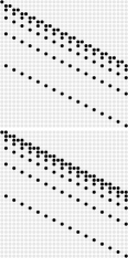
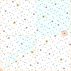
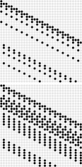
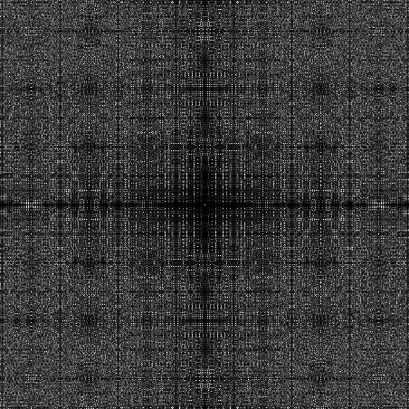
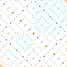
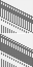
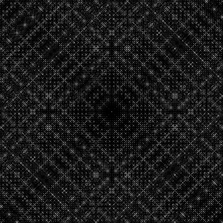
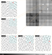
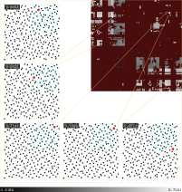
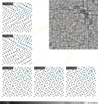
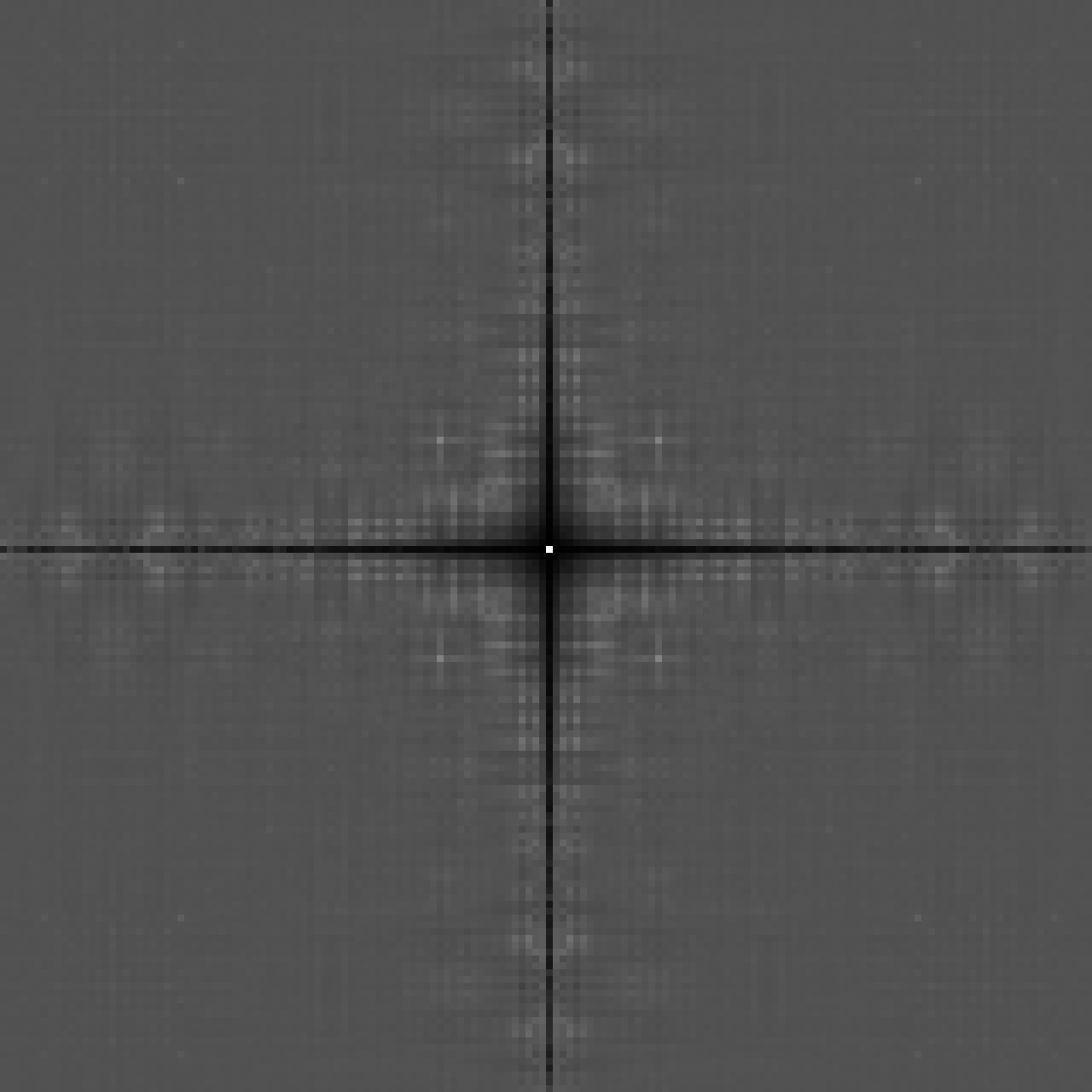
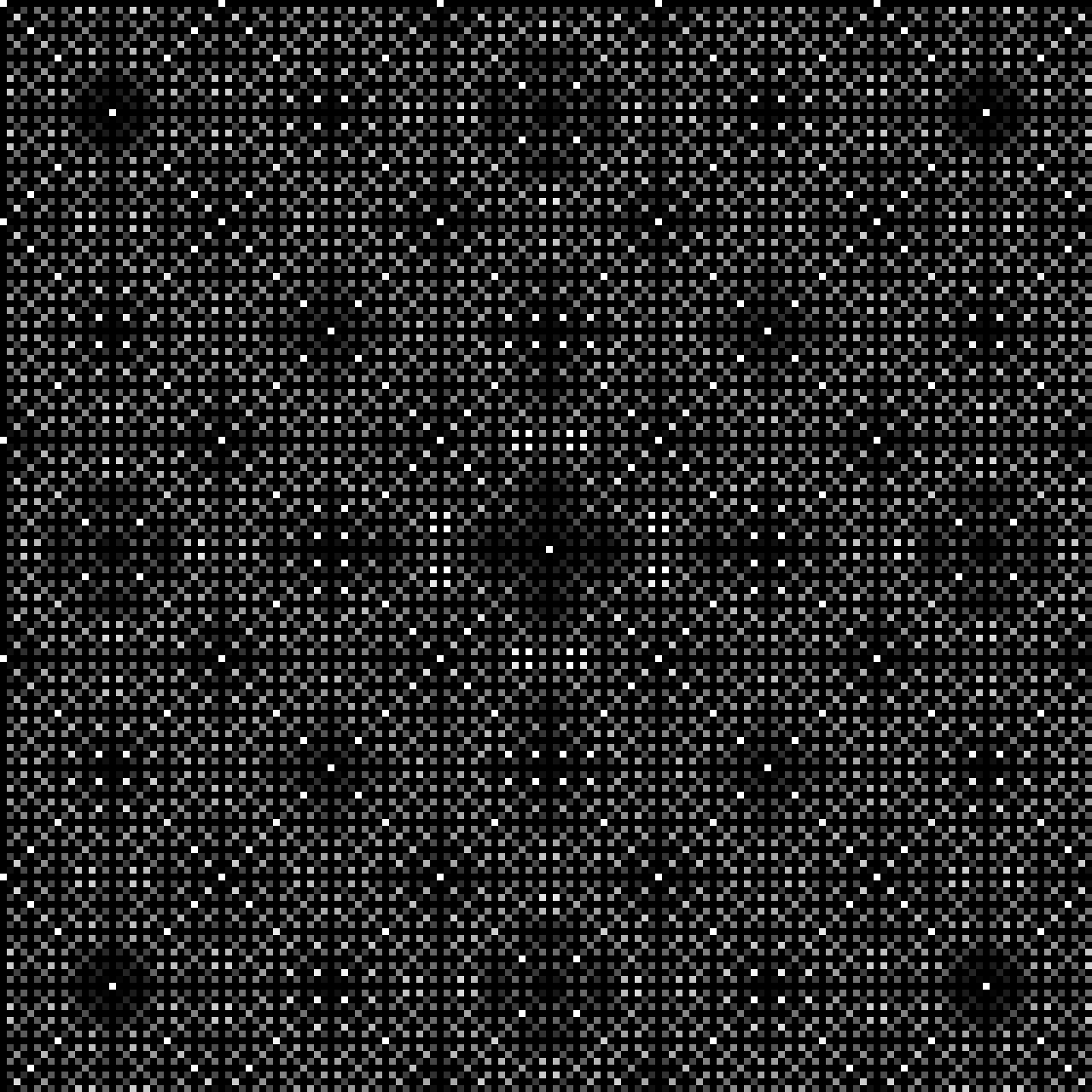
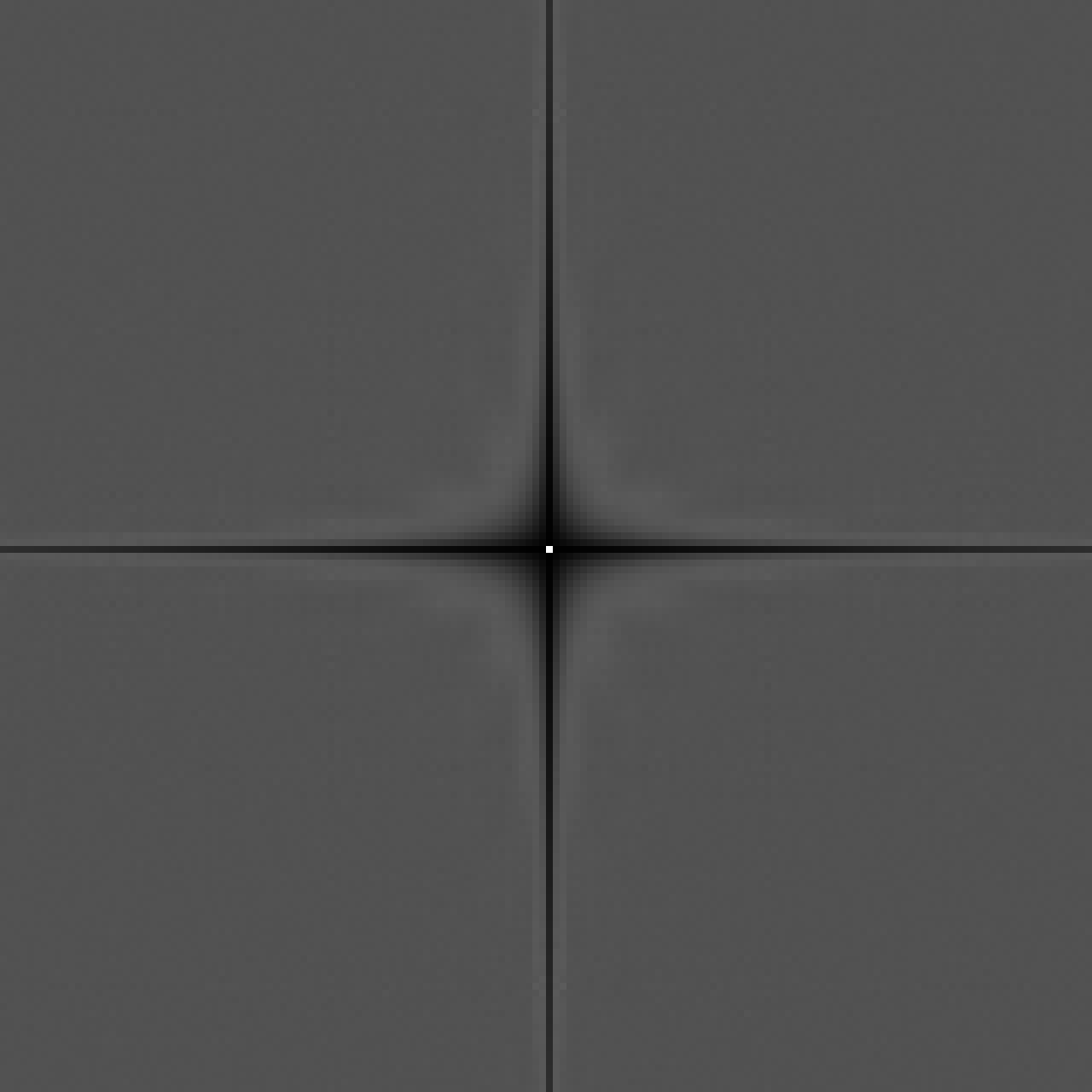
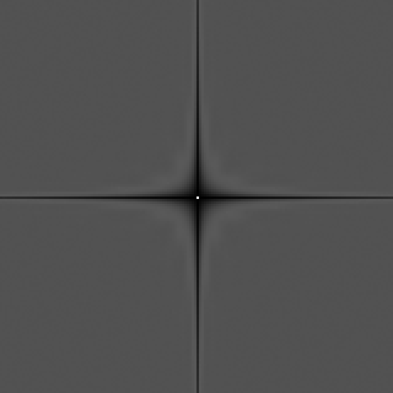
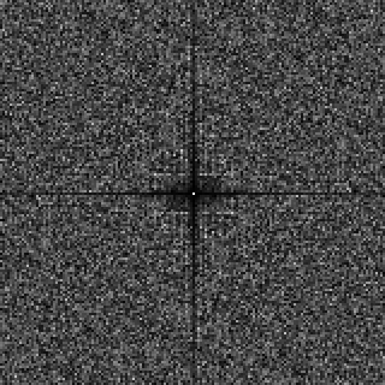
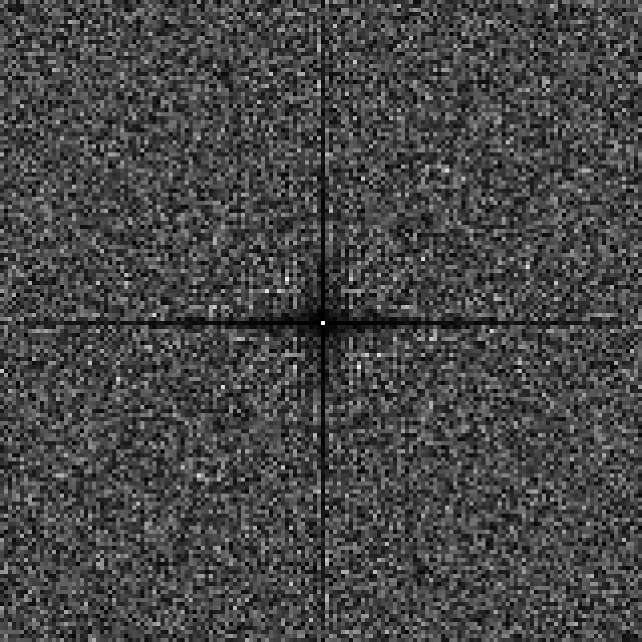
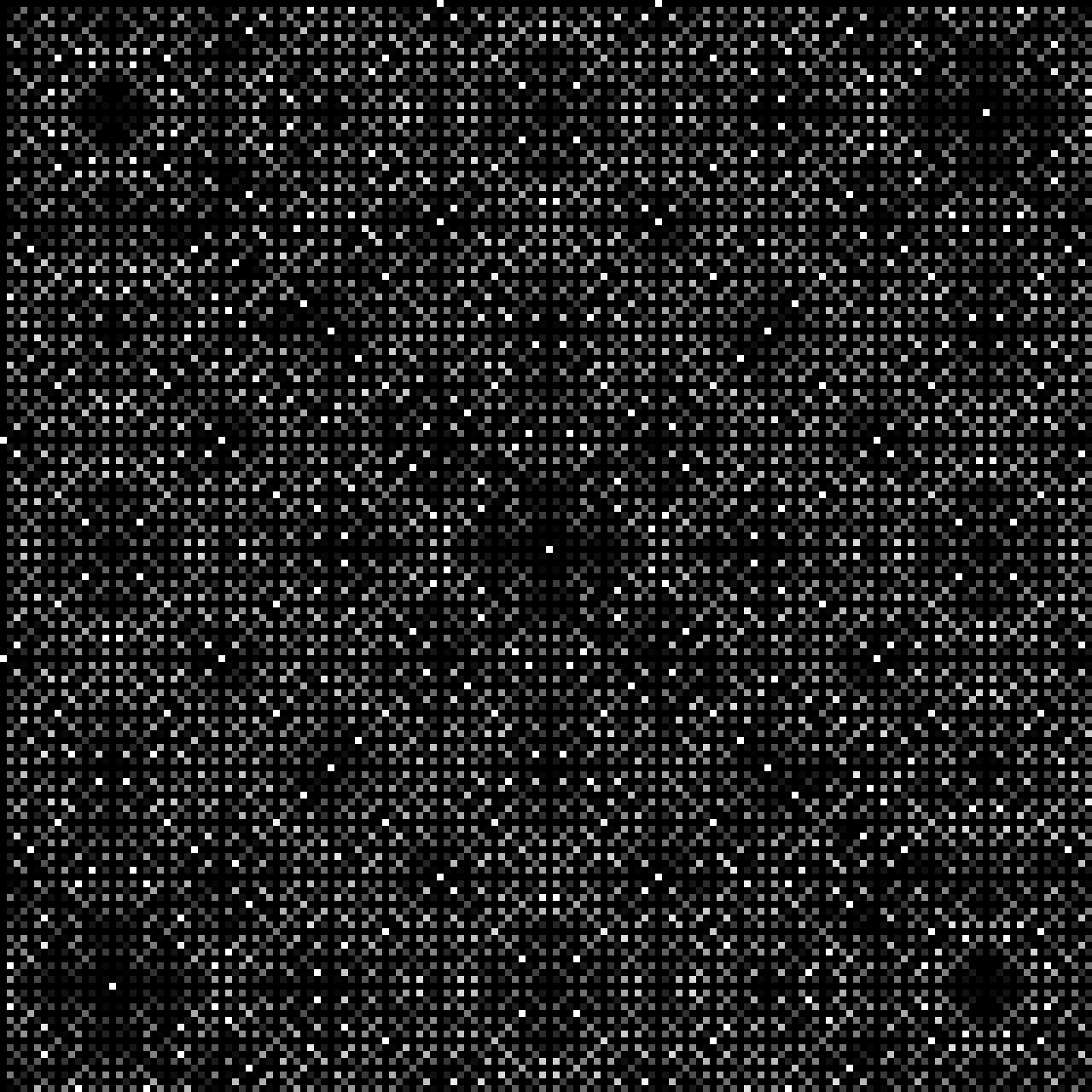
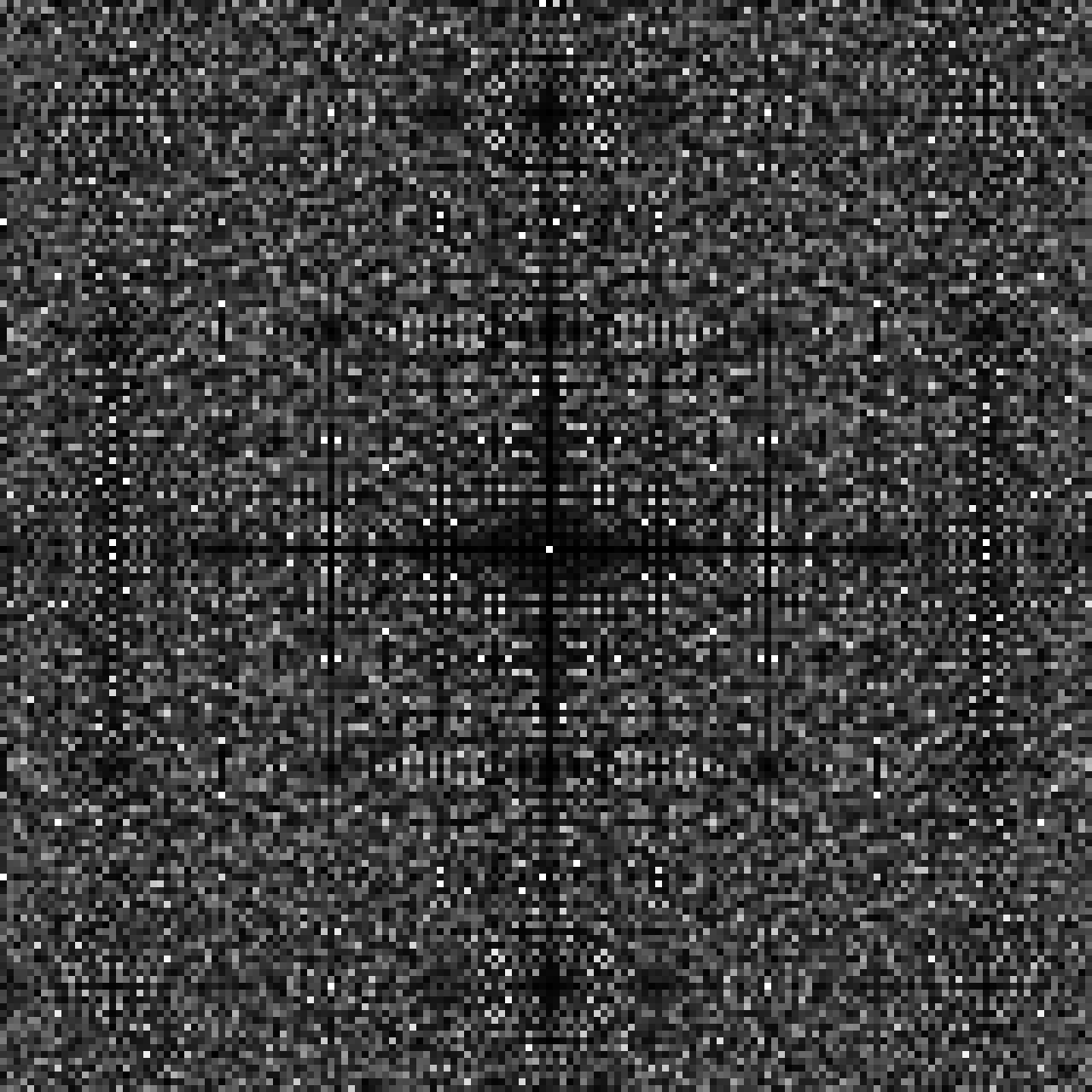
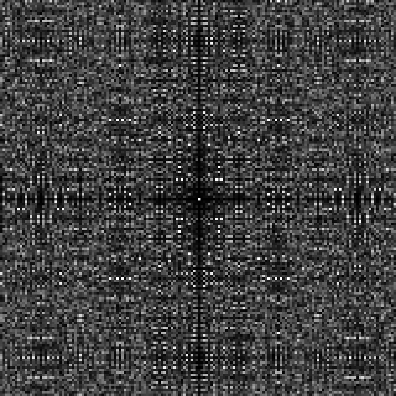
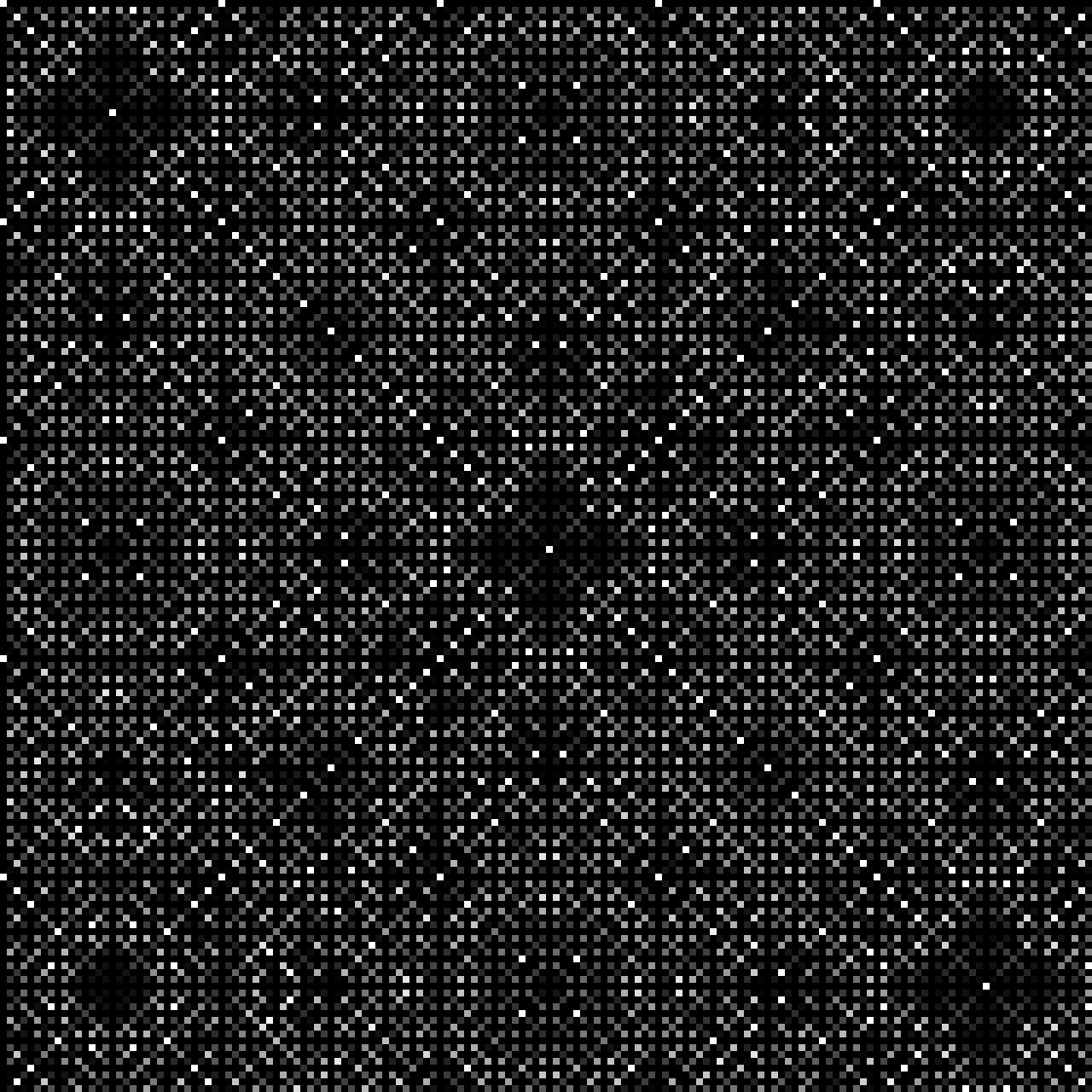
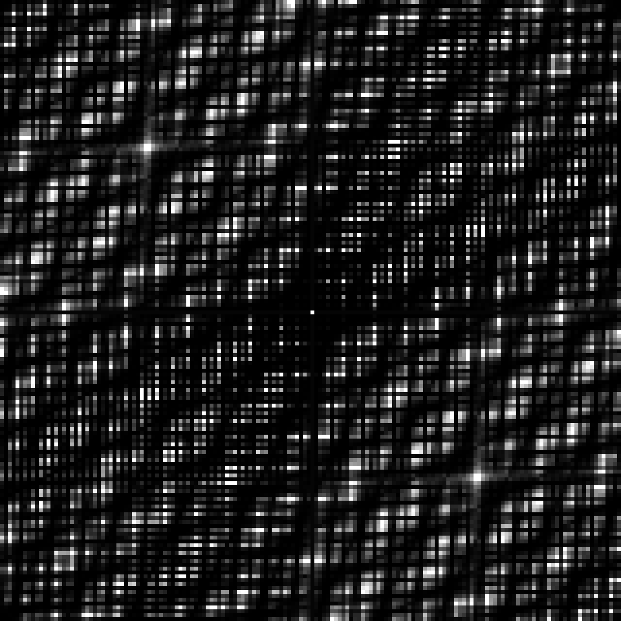
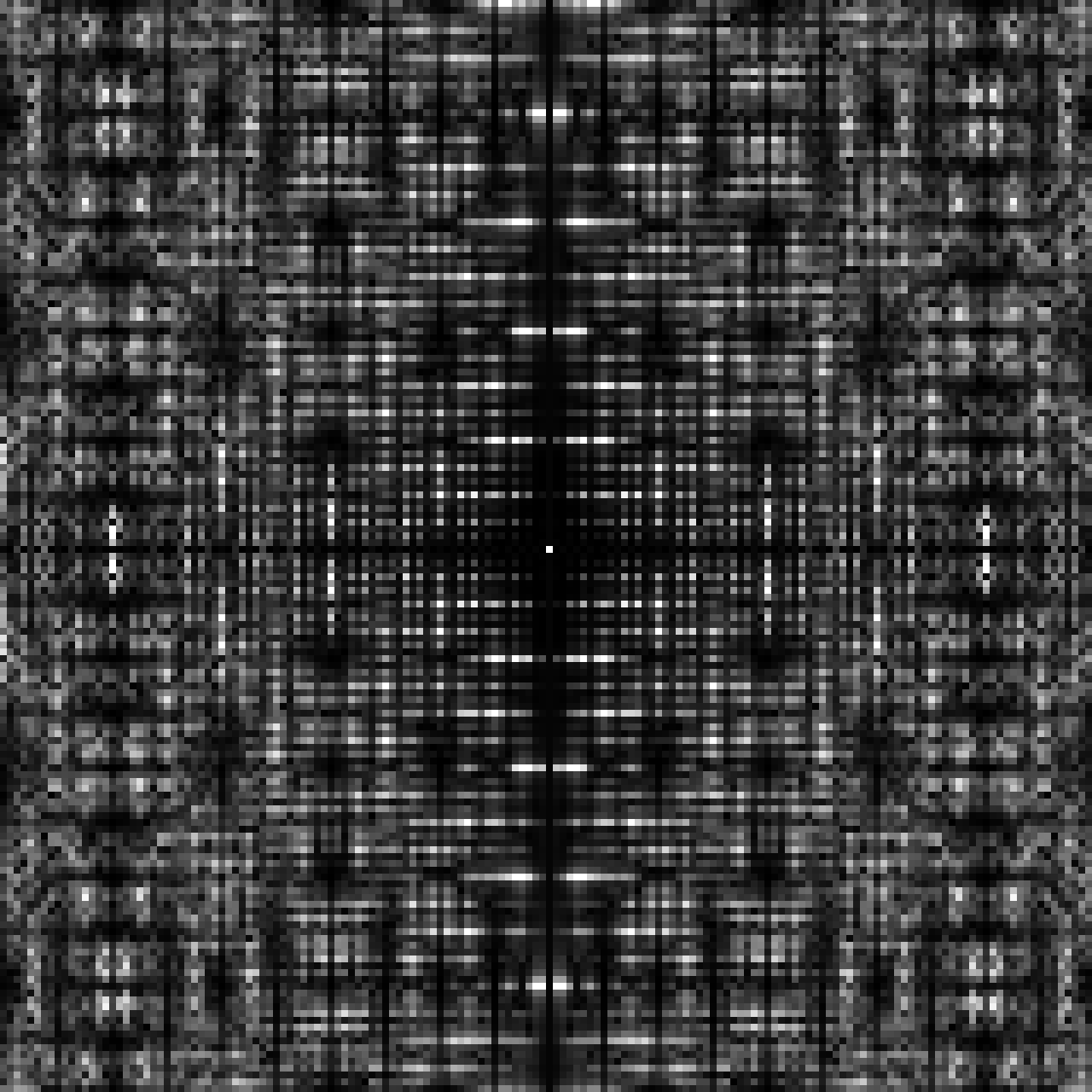
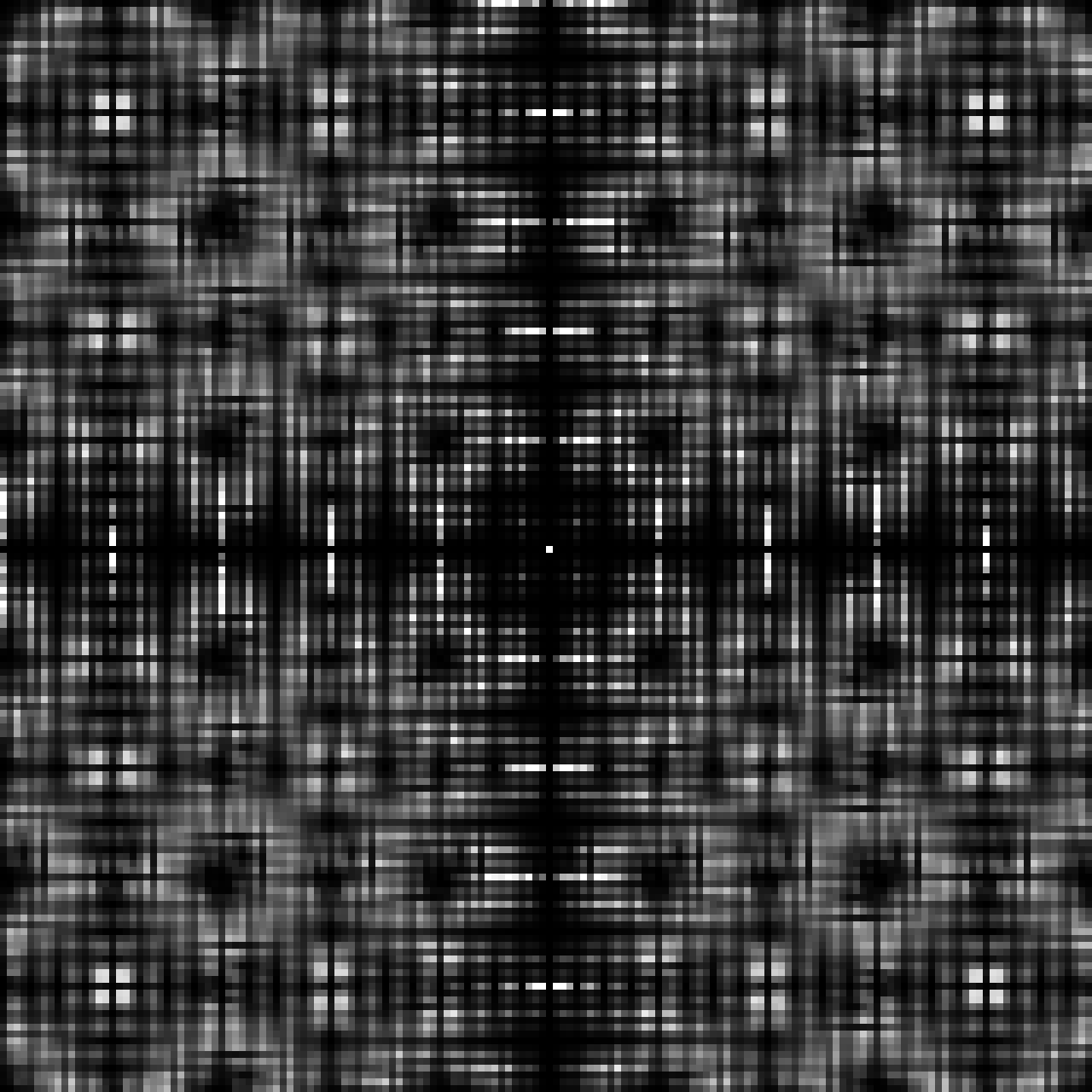
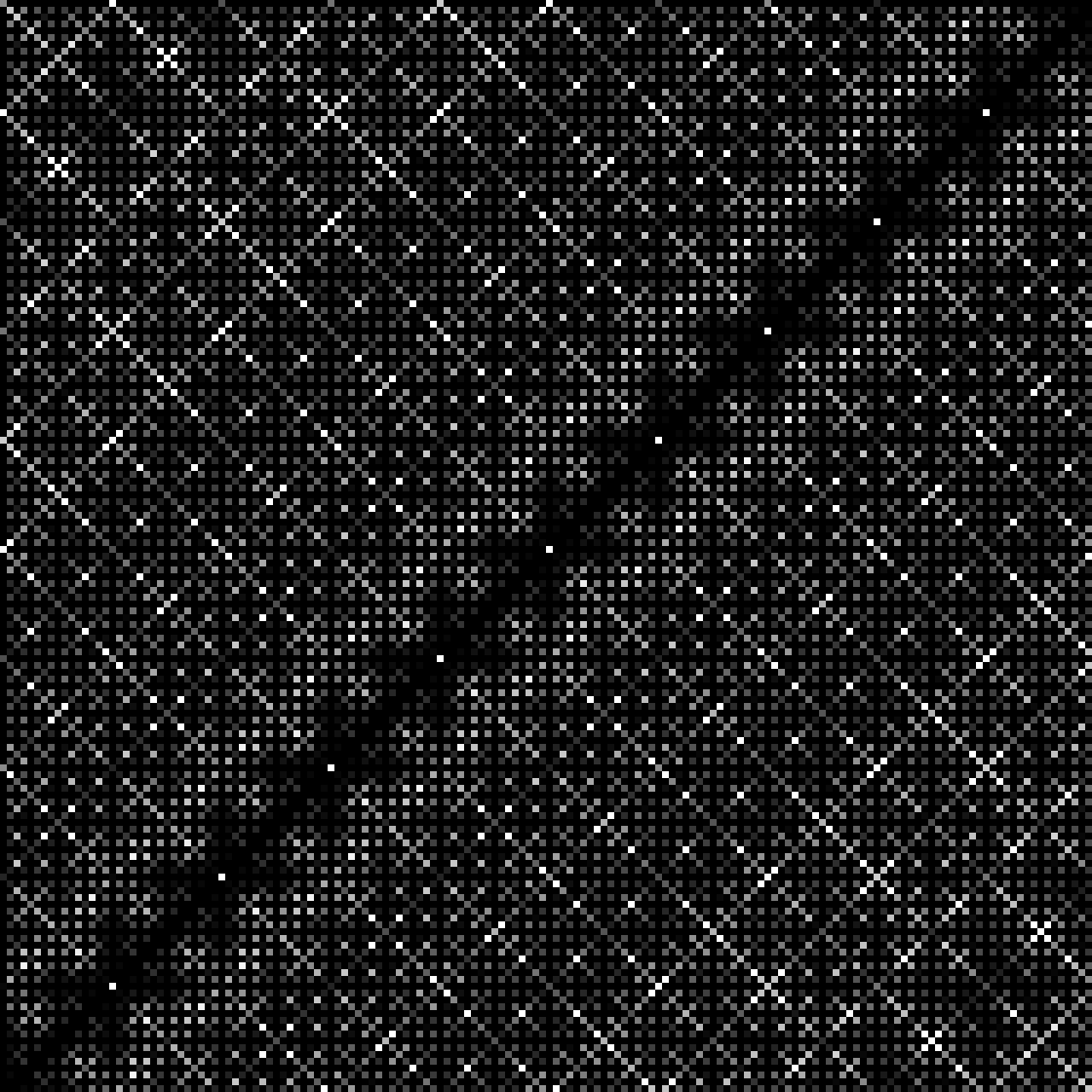
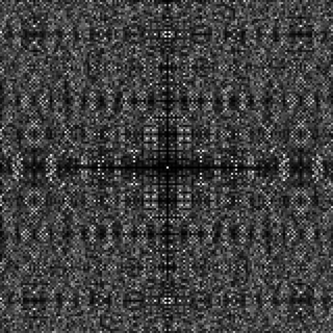
Figure 1. Generating matrices, points, and periodograms of various digital dyadic sequences. The first 2msuperscript2𝑚2^{m} points of the sequences are shown for m=0,,9𝑚09m=0,\dots,9 in separate squares of increasing sizes. The digital dyadic sequences in (b) and (c) are obtained by reordering the known digital dyadic nets with the same names; such reordering is one of the main discoveries of the paper. The sequence in (d) is obtained from a 256256256-point Gray net by first reordering it into a sequence and then extending the sequence in one of the possible ways. The sequence in (e) represents a new class of self-similar sequences introduced in the paper.

1. Introduction

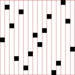
Sampling is a fundamental process in computer graphics, underlying Monte Carlo integration in rendering, halftoning, stippling, generative modeling, and object distributions. A wide range of sampling strategies have been developed, and none is conclusively considered the best so far. Low-discrepancy patterns, however, introduced by Shirley (1991) to graphics and popularized mostly by Keller and collaborators, are arguably leading the competition for use in rendering. Of special interest are so-called dyadic nets and sequences, mainly the Hammersley net and the Sobol sequence. These combine exceptionally high production rates with excellent convergence behavior when used in Monte Carlo integration, for which they are specifically designed. They are very versatile, as described in the discussion by Keller (2013). Furthermore, they are easy to understand thanks to their modular geometric “multi-stratified” structure (Pharr et al., 2016). In a nutshell, a dyadic net is concerned with a “fair” 2D distribution of N=2m𝑁superscript2𝑚N=2^{m} points, so that specifically constructed rectangles of equal area contain exactly one point. These rectangles are obtained by partitioning the unit square [0,1)2superscript012[0,1)^{2} into rectangular cells of sizes 12m×11superscript2𝑚1\frac{1}{2^{m}}\times 1, 12m1×121superscript2𝑚112\frac{1}{2^{m-1}}\times\frac{1}{2}, \ldots, 1×12m11superscript2𝑚1\times\frac{1}{2^{m}} (see Fig. 2). A dyadic sequence is a sequence of sample points such that all leading sub-sequences of points of size 2msuperscript2𝑚2^{m}, for all m𝑚m, are dyadic nets as well as all subsequent sub-sequences of size 2msuperscript2𝑚2^{m} (see Fig. 3). We would like to remark that dyadic nets and sequences fulfill the weaker n𝑛n-rooks and Latin hypercube conditions so that they are proper subsets. In computer graphics, the research effort in the area of dyadic nets and sequences was spearheaded by Keller and collaborators, who early on used and analyzed dyadic distributions in rendering (Kollig and Keller, 2002; Keller, 2006; Grünschloß et al., 2008; Grünschloß and Keller, 2009).

In this paper, we set out to analyze the design space of matrix-generated, or digital, dyadic nets and sequences. One possible reason why this design space is still not fully explored is that the focus of the Monte Carlo community might have been on proving discrepancy bounds and not the actual construction of dyadic sequences and dyadic nets. Therefore, important contributions in the area of sample construction were made even recently. Examples include a compact parametrization of the whole dyadic space by Ahmed and Wonka (2021), a compact parametrization of a sub-space comprising dyadic sequences, along with a very efficient generation algorithm, by Helmer et al. (2021), and an all-new construction of a high-dimensional distribution that has pair-wise two-dimensional projections by Paulin et al. (2021).

Our paper makes the following contributions:

  • a comprehensive analysis of digital dyadic nets and sequences. We introduce the missing ingredient (Thm. 3.8) that enables us to map the analysis of matrices generating digital dyadic sequences to the language of linear algebra.

  • the computation of the exact dimension of the design space for both digital dyadic nets and sequences.

  • an algorithm that reorders any digital dyadic net into a digital dyadic sequence. For example, we can reorder the Hammersley net or the Larcher-Pillichshammer net into digital dyadic sequences.

  • the discovery of self-similar dyadic sequences, also called ξ𝜉\xi-sequences. They are more efficient to construct than the Sobol sequence, and they are easily invertible. The subspace of ξ𝜉\xi-sequences is large enough to contain examples with low discrepancy and a large minimal distance between two sample points.
Refer to caption Refer to caption Refer to caption Refer to caption Refer to caption
116×11161\frac{1}{16}\times 1 18×121812\frac{1}{8}\times\frac{1}{2} 14×141414\frac{1}{4}\times\frac{1}{4} 12×181218\frac{1}{2}\times\frac{1}{8} 1×11611161\times\frac{1}{16}
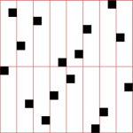
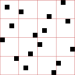
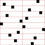
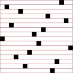
Figure 2. An example 4-bit 16-point dyadic net (i.e., m=4𝑚4m=4, N=16𝑁16N=16) showing all m+1=5𝑚15m+1=5 possible stratifications: 124×11superscript241\frac{1}{2^{4}}\times 1, 123×121superscript2312\frac{1}{2^{3}}\times\frac{1}{2}, 122×1221superscript221superscript22\frac{1}{2^{2}}\times\frac{1}{2^{2}}, 12×123121superscript23\frac{1}{2}\times\frac{1}{2^{3}}, 1×12411superscript241\times\frac{1}{2^{4}}.
Refer to caption
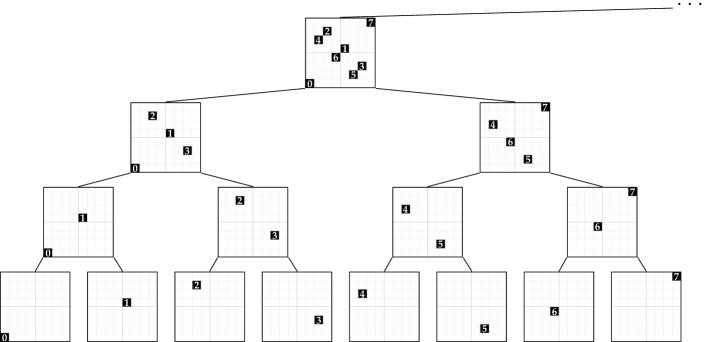
Figure 3. The hierarchical structure of a dyadic sequence is visualized as a tree. Note that the individual points also represent (0, 0, 2)-nets (i.e., 1-point dyadic nets). All sub-sequences corresponding to an internal (or leaf) node in the tree are required to be dyadic nets. Here the gray midlines are shown for better appearance.

The rest of the paper is organized as follows. In Section 2, we highlight the most relevant literature. In Section 3, we define and analyze digital dyadic nets and sequences, recall some known and state our new theoretical results: compute the exact dimension of the design space for both and give an algorithm that reorders any digital dyadic net into a digital dyadic sequence. In Section 4, we apply our algorithm for several examples: we reorder the Hammersley, the Larcher–Pillichshammer, and the Gray nets into digital dyadic sequences. In Section 5, we introduce and study new self-similar dyadic sequences and give an explicit parametrization of their design space.

2. Related Work

Our work has interesting connections to different fields of study in computer graphics and mathematics. In this section, we try to highlight the most relevant literature, organized into three categories.

2.1. Low-Discrepancy Sampling

The study of uniform sample distributions is much older than computer graphics. An early 1D sequence was presented by van der Corput (1935), who established the digit-reversal principle that underlies almost all Low-Discrepancy (LD) constructions. Roth (1954) and Hammersley (1960), respectively, presented techniques for extending the van der Corput principle to two and higher dimensions.

In a parallel line of study, Sobol (1967) pioneered the digital construction of LD sets and sequences, generalized by Niederreiter (1987; 1992), who coined the terms (t,m,s)𝑡𝑚𝑠(t,m,s)-nets and (t,s)𝑡𝑠(t,s)-sequences, and initiated a new field of study of these constructions. We defer definitions to Section 3, but point out that nets are finite LD sets, while sequences are extensible sets that admit more points while maintaining a low discrepancy. Most of these constructions are digital, i.e. sample coordinates are derived from the sequence number via binary matrix vector multiplication and vector addition modulo 222. A thorough study of common construction methods is given by Dick and Pillichshammer (2010). Not all nets and sequences, however, are necessarily digital, and there are known algorithms for constructing non-digital nets (Grünschloß and Keller, 2009; Ahmed and Wonka, 2021).

Aside from direct construction techniques of nets and sequences, Owen (1995; 1998) presented a powerful technique to randomize (t,m,s)𝑡𝑚𝑠(t,m,s)-nets and (t,s)𝑡𝑠(t,s)-sequences while preserving their favorable properties; in fact improving their quality. The original concept by Owen, while quite simple, is very memory intensive, consuming as many random bits—per dimension—as the number of samples. Much work followed Owen’s, mainly aimed at simplifications for more efficient implementation (Friedel and Keller, 2002; Kollig and Keller, 2002; Burley, 2020), at the cost of different compromises. However, there are also variants that are conceptually different; most notably the techniques of Faure and Tezuka (2002) aimed at shuffling the order of the samples rather than scrambling their locations.

Owen’s scrambling works only on existing nets and sequences, so a method for generating the underlying sets is still required. Ahmed and Wonka (2021) presented a technique for the direct construction of arbitrary 2D nets, but their method can only produce nets and consumes even more random bits than Owen’s scrambling.

2.2. Recursive Tiling Techniques

Ostromoukhov (2007) is credited for importing the digit-reversal principle of LD constructions (Section 2.1) and using it to distribute blue-noise samples over a self-similar set of tiles. The idea was followed up by Wachtel et al. (2014), and matured in Ahmed et al. (2017), whose tile set, ART, has a low granularity and tuneable properties, presenting a comparable blue-noise competitor to LD sequences (Christensen et al., 2018; Ahmed and Wonka, 2021; Kopf et al., 2006).

2.3. Low-Discrepancy Blue Noise

A recent trend of research tries to inject blue noise properties into LD sets and/or sequences. Early ideas along this line of research may be traced back to Keller (2006), who speculated on the superiority of LD sets that bear a large minimum distance between points, showcasing the very-low-discrepancy family of nets by Larcher and Pillichshammer (2003) that also attain a large minimum distance between points. Grünschloß and colleagues subsequently presented examples of small-sized digital nets with maximized minimum distance between points obtained via a search algorithm (2008), as well as non-digital constructions developed heuristically (2009). The recent work of Christensen et al. (2018), along with (Pharr et al., 2016; Helmer et al., 2021), may be seen as an extension of this search approach that targets sequences instead of nets.

A different line of research in this category was that of Ahmed et al. (2016), with an algorithm for proactively imposing spectral control over LD nets, at the cost of compromising the quality of the net. Perrier et al. (2018) extended this idea to sequences. See a survey by Singh et al. (2019) for details. Ahmed and Wonka (2021) demonstrated the possibility of incorporating spectral control into nets without compromising their quality but highlighted the difficulty of extending the idea to sequences.

3. Analysis of Digital Dyadic Nets and Sequences

In this section, we define and analyze digital dyadic nets and sequences, and state our new theoretical results: computation of the exact dimension of the design space for both and an algorithm that reorders any digital dyadic net into a digital dyadic sequence.

3.1. Definitions

There is a general notion of (t,m,s)𝑡𝑚𝑠(t,m,s)-nets in base b𝑏b. In this paper, we are focused on the particular case of 2D dyadic nets. They are known as (0,m,2)0𝑚2(0,m,2)-nets in base 2 (in short, m𝑚m-nets, or 2msuperscript2𝑚2^{m}-point nets). Further, we specifically study dyadic sequences, also known as (0,2)02(0,2)-sequences in base 222.

Definition 3.0.

By a rectangle a×b𝑎𝑏a\times b we mean the set of points

{(x,y)2:x0x<x0+a,y0y<y0+b}for some x0,y0.conditional-set𝑥𝑦superscript2formulae-sequencesubscript𝑥0𝑥subscript𝑥0𝑎subscript𝑦0𝑦subscript𝑦0𝑏for some x0,y0.\{\,(x,y)\in\mathbb{R}^{2}:x_{0}\leq x<x_{0}+a,\,y_{0}\leq y<y_{0}+b\,\}\quad\text{for some $x_{0},y_{0}$.}

Consider m+1𝑚1m+1 possible stratifications of the unit square [0,1)2superscript012[0,1)^{2} into equal rectangles 12m×11superscript2𝑚1\frac{1}{2^{m}}\times 1, 12m1×121superscript2𝑚112\frac{1}{2^{m-1}}\times\frac{1}{2}, \ldots, 1×12m11superscript2𝑚1\times\frac{1}{2^{m}} (strata). See Fig. 2. A 2msuperscript2𝑚2^{m}-point set in [0,1)2superscript012[0,1)^{2} is a dyadic net if it contains a single point per stratum in each of the m+1𝑚1m+1 stratifications.

A dyadic sequence is a finite or infinite sequence of points in [0,1)2superscript012[0,1)^{2} such that the first 2msuperscript2𝑚2^{m} points, the next 2msuperscript2𝑚2^{m} points, and all subsequent blocks of 2msuperscript2𝑚2^{m} points are dyadic nets for all m=0,1,𝑚01m=0,1,\ldots.

Thus, infinite dyadic sequences comprise sequences of dyadic nets of all sizes. Any dyadic sequence can be visualized as a binary tree, where each node corresponds to a dyadic net. See Fig. 3.

Now we turn to digital dyadic nets (Niederreiter, 1987). Hereafter all the computations use linear algebra over the Galois field GF(2)𝐺𝐹2GF(2), also denoted by /22\mathbb{Z}/2\mathbb{Z} or 2subscript2\mathbb{Z}_{2}: all vector and matrix entries {0,1}absent01\in\{0,1\} and 1+1=01101+1=0. Computation in GF(2)𝐺𝐹2GF(2) is different from computing with binary matrices over the real numbers (1+1=21121+1=2), or Boolean algebra (1+1=11111+1=1). In what follows, a matrix refers to an m×m𝑚𝑚m\times m matrix with the entries in GF(2)𝐺𝐹2GF(2) unless otherwise indicated.

Definition 3.0.

For two bit vectors X=(x1,,xm)𝑋subscript𝑥1subscript𝑥𝑚X=(x_{1},\dots,x_{m}) and Y=(y1,,ym)𝑌subscript𝑦1subscript𝑦𝑚Y=(y_{1},\dots,y_{m}), denote ρ(X,Y):=(0.x1xm,0.y1ym)[0,1)2\rho(X,Y):=(0.x_{1}\dots x_{m},0.y_{1}\dots y_{m})\in[0,1)^{2}. An ordered collection of 2msuperscript2𝑚2^{m} distinct points (X1,Y1)subscript𝑋1subscript𝑌1(X_{1},Y_{1}), (X2,Y2)subscript𝑋2subscript𝑌2(X_{2},Y_{2}), …is called digital if

(1) (Xi,Yi)=ρ(CxSi,CySi),subscript𝑋𝑖subscript𝑌𝑖𝜌subscript𝐶𝑥subscript𝑆𝑖subscript𝐶𝑦subscript𝑆𝑖(X_{i},Y_{i})=\rho(C_{x}S_{i},C_{y}S_{i})\,,

where (Cx,Cy)subscript𝐶𝑥subscript𝐶𝑦(C_{x},C_{y}) is a fixed pair of binary m×m𝑚𝑚m\times m matrices, S1subscript𝑆1S_{1}, S2subscript𝑆2S_{2}, …enumerate all the binary m𝑚m-bit column vectors in the order (0,,0)00(0,\dots,0), (1,0,,0)100(1,0,\dots,0), (0,1,,0)010(0,1,\dots,0), …, (1,,1)11(1,\dots,1), and the products are modulo 222.

A digital collection of points that is also a dyadic net (sequence) is called a digital dyadic net (sequence).

Equivalently, based on the analysis from (Ahmed and Wonka, 2021), a digital collection of points is a digital dyadic net, if it contains a unique point ρ(X,Y)𝜌𝑋𝑌\rho(X,Y) with any given last r𝑟r bits of X𝑋X and last mr𝑚𝑟m-r bits of Y𝑌Y, for each r=0,1,,m𝑟01𝑚r=0,1,\dots,m. Likewise, a digital collection of points is a digital dyadic sequence, if the first and all the subsequent blocks of 2ksuperscript2𝑘2^{k} points form a digital dyadic net after removing the last mk𝑚𝑘m-k bits from both X𝑋X and Y𝑌Y, for each k<m𝑘𝑚k<m.

Table 1. Overview of constructions of different digital dyadic nets and sequences. Lx,Lysubscript𝐿𝑥subscript𝐿𝑦L_{x},L_{y} are lower unitriangular matrices, Ux,Uysubscript𝑈𝑥subscript𝑈𝑦U_{x},U_{y} are upper unitriangular matrices, J𝐽J is the anti-diagonal matrix with all ones on the anti-diagonal, P𝑃P is the binary Pascal matrix, M𝑀M is any invertible matrix, X0,Y0subscript𝑋0subscript𝑌0X_{0},Y_{0} are binary bit vectors, and S𝑆S is the index of the generated point (X,Y)𝑋𝑌(X,Y) in binary bit vector form. See Section 4 for details.
Name of construction Explicit construction # constructions (counting permutations) # constructions (not counting permutations)
Digital dyadic nets (X,Y)=(M,LyUyJM)S𝑋𝑌𝑀subscript𝐿𝑦subscript𝑈𝑦𝐽𝑀𝑆(X,Y)=(M,L_{y}U_{y}JM)S 23m(m1)/2(211)(221)(2m1)superscript23𝑚𝑚12superscript211superscript221superscript2𝑚12^{3m(m-1)/2}(2^{1}-1)(2^{2}-1)\cdots(2^{m}-1) 2m(m1)superscript2𝑚𝑚12^{m(m-1)}
GS-nets (X,Y)=(LxM,LyPM)S𝑋𝑌subscript𝐿𝑥𝑀subscript𝐿𝑦𝑃𝑀𝑆(X,Y)=(L_{x}M,L_{y}PM)S 23m(m1)/2(211)(221)(2m1)superscript23𝑚𝑚12superscript211superscript221superscript2𝑚12^{3m(m-1)/2}(2^{1}-1)(2^{2}-1)\cdots(2^{m}-1) 2m(m1)superscript2𝑚𝑚12^{m(m-1)}
Digital dyadic sequences (X,Y)=(LxUx,LyPUx)S𝑋𝑌subscript𝐿𝑥subscript𝑈𝑥subscript𝐿𝑦𝑃subscript𝑈𝑥𝑆(X,Y)=(L_{x}U_{x},L_{y}PU_{x})S 23m(m1)/2superscript23𝑚𝑚122^{3m(m-1)/2} 2m(m1)superscript2𝑚𝑚12^{m(m-1)}
GFaure sequences (X,Y)=(Lx,LyP)S𝑋𝑌subscript𝐿𝑥subscript𝐿𝑦𝑃𝑆(X,Y)=(L_{x},L_{y}P)S 2m(m1)superscript2𝑚𝑚12^{m(m-1)} 2m(m1)superscript2𝑚𝑚12^{m(m-1)}
Hammersley-like nets (X,Y)=(J,LyUy)S𝑋𝑌𝐽subscript𝐿𝑦subscript𝑈𝑦𝑆(X,Y)=(J,L_{y}U_{y})S 2m(m1)superscript2𝑚𝑚12^{m(m-1)} 2m(m1)superscript2𝑚𝑚12^{m(m-1)}
Affine digital dyadic nets (X,Y)=(M,LyUyJM)S+(X0,Y0)𝑋𝑌𝑀subscript𝐿𝑦subscript𝑈𝑦𝐽𝑀𝑆subscript𝑋0subscript𝑌0(X,Y)=(M,L_{y}U_{y}JM)S+(X_{0},Y_{0}) 2m(3m+1)/2(211)(221)(2m1)superscript2𝑚3𝑚12superscript211superscript221superscript2𝑚12^{m(3m+1)/2}(2^{1}-1)(2^{2}-1)\cdots(2^{m}-1) 2m2superscript2superscript𝑚22^{m^{2}}
Affine digital dyadic sequences (X,Y)=(LxUx,LyPUx)S+(X0,Y0)𝑋𝑌subscript𝐿𝑥subscript𝑈𝑥subscript𝐿𝑦𝑃subscript𝑈𝑥𝑆subscript𝑋0subscript𝑌0(X,Y)=(L_{x}U_{x},L_{y}{P}U_{x})S+(X_{0},Y_{0}) 2m(3m+1)/2superscript2𝑚3𝑚122^{m(3m+1)/2} 2m2superscript2superscript𝑚22^{m^{2}}
Table 2. Overview of constructions of particular digital dyadic nets and sequences. I𝐼I and J𝐽J are the identity and anti-diagonal matrices, respectively. P𝑃{P} is the binary Pascal matrix. ULPsubscript𝑈LPU_{\mathrm{LP}} and LLPsubscript𝐿LPL_{\mathrm{LP}} are given by (3) and (11). S𝑆S is the index of the generated point (X,Y)𝑋𝑌(X,Y) in binary bit vector form.
Name of construction Explicit construction
Sobol (Faure) sequence (X,Y)=(I,P)S𝑋𝑌𝐼𝑃𝑆(X,Y)=(I,{P})S
Hammersley net (X,Y)=(J,I)S𝑋𝑌𝐽𝐼𝑆(X,Y)=(J,I)S
Hammersley sequence (X,Y)=(JPJ,PJ)S𝑋𝑌𝐽𝑃𝐽𝑃𝐽𝑆(X,Y)=(JPJ,PJ)S
LP net (X,Y)=(J,ULP)S𝑋𝑌𝐽subscript𝑈LP𝑆(X,Y)=(J,U_{\mathrm{LP}})S
LP sequence (X,Y)=(LLP,PJ)S𝑋𝑌subscript𝐿LP𝑃𝐽𝑆(X,Y)=(L_{\mathrm{LP}},PJ)S

This notation enables us to express well-known sequences and nets in succinct form; the map “ρ𝜌\rho” is usually omitted. Table 1 summarizes explicit parametrizations of digital dyadic nets and sequences, and the analysis of how many different constructions are possible by each parametrization. The GFaure construction introduced by Tezuka (1994) describes a family of sequences obtained by setting Cx=Lxsubscript𝐶𝑥subscript𝐿𝑥C_{x}=L_{x} and Cy=LyPsubscript𝐶𝑦subscript𝐿𝑦𝑃C_{y}=L_{y}{P}, with Lxsubscript𝐿𝑥L_{x} and Lysubscript𝐿𝑦L_{y} arbitrary lower unitriangular matrices and P𝑃{P} the binary Pascal matrix. By a unitriangular matrix we mean an upper or lower triangular matrix with all ones on the diagonal. The entries of the Pascal matrix P𝑃{P} are Pij=(j1i1)mod2subscript𝑃𝑖𝑗modulobinomial𝑗1𝑖12{P}_{ij}=\binom{j-1}{i-1}\mod 2, with i𝑖i row and j𝑗j column index, respectively:

(2) P=(1111111101010101001100110001000100001111000001010000001100000001).𝑃1111111101010101001100110001000100001111000001010000001100000001{P}=\left(\begin{array}[]{ccccccccc}1&1&1&1&1&1&1&1&\cdots\\ \color[rgb]{.75,.75,.75}\definecolor[named]{pgfstrokecolor}{rgb}{.75,.75,.75}\pgfsys@color@gray@stroke{.75}\pgfsys@color@gray@fill{.75}0&1&\color[rgb]{.75,.75,.75}\definecolor[named]{pgfstrokecolor}{rgb}{.75,.75,.75}\pgfsys@color@gray@stroke{.75}\pgfsys@color@gray@fill{.75}0&1&\color[rgb]{.75,.75,.75}\definecolor[named]{pgfstrokecolor}{rgb}{.75,.75,.75}\pgfsys@color@gray@stroke{.75}\pgfsys@color@gray@fill{.75}0&1&\color[rgb]{.75,.75,.75}\definecolor[named]{pgfstrokecolor}{rgb}{.75,.75,.75}\pgfsys@color@gray@stroke{.75}\pgfsys@color@gray@fill{.75}0&1&\cdots\\ \color[rgb]{.75,.75,.75}\definecolor[named]{pgfstrokecolor}{rgb}{.75,.75,.75}\pgfsys@color@gray@stroke{.75}\pgfsys@color@gray@fill{.75}0&\color[rgb]{.75,.75,.75}\definecolor[named]{pgfstrokecolor}{rgb}{.75,.75,.75}\pgfsys@color@gray@stroke{.75}\pgfsys@color@gray@fill{.75}0&1&1&\color[rgb]{.75,.75,.75}\definecolor[named]{pgfstrokecolor}{rgb}{.75,.75,.75}\pgfsys@color@gray@stroke{.75}\pgfsys@color@gray@fill{.75}0&\color[rgb]{.75,.75,.75}\definecolor[named]{pgfstrokecolor}{rgb}{.75,.75,.75}\pgfsys@color@gray@stroke{.75}\pgfsys@color@gray@fill{.75}0&1&1&\cdots\\ \color[rgb]{.75,.75,.75}\definecolor[named]{pgfstrokecolor}{rgb}{.75,.75,.75}\pgfsys@color@gray@stroke{.75}\pgfsys@color@gray@fill{.75}0&\color[rgb]{.75,.75,.75}\definecolor[named]{pgfstrokecolor}{rgb}{.75,.75,.75}\pgfsys@color@gray@stroke{.75}\pgfsys@color@gray@fill{.75}0&\color[rgb]{.75,.75,.75}\definecolor[named]{pgfstrokecolor}{rgb}{.75,.75,.75}\pgfsys@color@gray@stroke{.75}\pgfsys@color@gray@fill{.75}0&1&\color[rgb]{.75,.75,.75}\definecolor[named]{pgfstrokecolor}{rgb}{.75,.75,.75}\pgfsys@color@gray@stroke{.75}\pgfsys@color@gray@fill{.75}0&\color[rgb]{.75,.75,.75}\definecolor[named]{pgfstrokecolor}{rgb}{.75,.75,.75}\pgfsys@color@gray@stroke{.75}\pgfsys@color@gray@fill{.75}0&\color[rgb]{.75,.75,.75}\definecolor[named]{pgfstrokecolor}{rgb}{.75,.75,.75}\pgfsys@color@gray@stroke{.75}\pgfsys@color@gray@fill{.75}0&1&\cdots\\ \color[rgb]{.75,.75,.75}\definecolor[named]{pgfstrokecolor}{rgb}{.75,.75,.75}\pgfsys@color@gray@stroke{.75}\pgfsys@color@gray@fill{.75}0&\color[rgb]{.75,.75,.75}\definecolor[named]{pgfstrokecolor}{rgb}{.75,.75,.75}\pgfsys@color@gray@stroke{.75}\pgfsys@color@gray@fill{.75}0&\color[rgb]{.75,.75,.75}\definecolor[named]{pgfstrokecolor}{rgb}{.75,.75,.75}\pgfsys@color@gray@stroke{.75}\pgfsys@color@gray@fill{.75}0&\color[rgb]{.75,.75,.75}\definecolor[named]{pgfstrokecolor}{rgb}{.75,.75,.75}\pgfsys@color@gray@stroke{.75}\pgfsys@color@gray@fill{.75}0&1&1&1&1&\cdots\\ \color[rgb]{.75,.75,.75}\definecolor[named]{pgfstrokecolor}{rgb}{.75,.75,.75}\pgfsys@color@gray@stroke{.75}\pgfsys@color@gray@fill{.75}0&\color[rgb]{.75,.75,.75}\definecolor[named]{pgfstrokecolor}{rgb}{.75,.75,.75}\pgfsys@color@gray@stroke{.75}\pgfsys@color@gray@fill{.75}0&\color[rgb]{.75,.75,.75}\definecolor[named]{pgfstrokecolor}{rgb}{.75,.75,.75}\pgfsys@color@gray@stroke{.75}\pgfsys@color@gray@fill{.75}0&\color[rgb]{.75,.75,.75}\definecolor[named]{pgfstrokecolor}{rgb}{.75,.75,.75}\pgfsys@color@gray@stroke{.75}\pgfsys@color@gray@fill{.75}0&\color[rgb]{.75,.75,.75}\definecolor[named]{pgfstrokecolor}{rgb}{.75,.75,.75}\pgfsys@color@gray@stroke{.75}\pgfsys@color@gray@fill{.75}0&1&\color[rgb]{.75,.75,.75}\definecolor[named]{pgfstrokecolor}{rgb}{.75,.75,.75}\pgfsys@color@gray@stroke{.75}\pgfsys@color@gray@fill{.75}0&1&\cdots\\ \color[rgb]{.75,.75,.75}\definecolor[named]{pgfstrokecolor}{rgb}{.75,.75,.75}\pgfsys@color@gray@stroke{.75}\pgfsys@color@gray@fill{.75}0&\color[rgb]{.75,.75,.75}\definecolor[named]{pgfstrokecolor}{rgb}{.75,.75,.75}\pgfsys@color@gray@stroke{.75}\pgfsys@color@gray@fill{.75}0&\color[rgb]{.75,.75,.75}\definecolor[named]{pgfstrokecolor}{rgb}{.75,.75,.75}\pgfsys@color@gray@stroke{.75}\pgfsys@color@gray@fill{.75}0&\color[rgb]{.75,.75,.75}\definecolor[named]{pgfstrokecolor}{rgb}{.75,.75,.75}\pgfsys@color@gray@stroke{.75}\pgfsys@color@gray@fill{.75}0&\color[rgb]{.75,.75,.75}\definecolor[named]{pgfstrokecolor}{rgb}{.75,.75,.75}\pgfsys@color@gray@stroke{.75}\pgfsys@color@gray@fill{.75}0&\color[rgb]{.75,.75,.75}\definecolor[named]{pgfstrokecolor}{rgb}{.75,.75,.75}\pgfsys@color@gray@stroke{.75}\pgfsys@color@gray@fill{.75}0&1&1&\cdots\\ \color[rgb]{.75,.75,.75}\definecolor[named]{pgfstrokecolor}{rgb}{.75,.75,.75}\pgfsys@color@gray@stroke{.75}\pgfsys@color@gray@fill{.75}0&\color[rgb]{.75,.75,.75}\definecolor[named]{pgfstrokecolor}{rgb}{.75,.75,.75}\pgfsys@color@gray@stroke{.75}\pgfsys@color@gray@fill{.75}0&\color[rgb]{.75,.75,.75}\definecolor[named]{pgfstrokecolor}{rgb}{.75,.75,.75}\pgfsys@color@gray@stroke{.75}\pgfsys@color@gray@fill{.75}0&\color[rgb]{.75,.75,.75}\definecolor[named]{pgfstrokecolor}{rgb}{.75,.75,.75}\pgfsys@color@gray@stroke{.75}\pgfsys@color@gray@fill{.75}0&\color[rgb]{.75,.75,.75}\definecolor[named]{pgfstrokecolor}{rgb}{.75,.75,.75}\pgfsys@color@gray@stroke{.75}\pgfsys@color@gray@fill{.75}0&\color[rgb]{.75,.75,.75}\definecolor[named]{pgfstrokecolor}{rgb}{.75,.75,.75}\pgfsys@color@gray@stroke{.75}\pgfsys@color@gray@fill{.75}0&\color[rgb]{.75,.75,.75}\definecolor[named]{pgfstrokecolor}{rgb}{.75,.75,.75}\pgfsys@color@gray@stroke{.75}\pgfsys@color@gray@fill{.75}0&1&\cdots\\ \vdots&\vdots&\vdots&\vdots&\vdots&\vdots&\vdots&\vdots&\ddots\end{array}\right)\,.

Hereafter a zero entry is in gray for readability.

Table 2 summarizes our newly introduced (see Section 4) as well as known constructions for reference, e.g. the Hammersley net is obtained by Cx=J,Cy=Iformulae-sequencesubscript𝐶𝑥𝐽subscript𝐶𝑦𝐼C_{x}={J},C_{y}={I}, with J𝐽{J} the anti-diagonal matrix with all ones on the anti-diagonal, and the Larcher–Pillichshammer (LP) net uses Cx=J,Cy=ULPformulae-sequencesubscript𝐶𝑥𝐽subscript𝐶𝑦subscript𝑈LPC_{x}={J},C_{y}=U_{\mathrm{LP}} with

(3) ULP=(1111011100110001).subscript𝑈LP1111011100110001U_{\mathrm{LP}}=\left(\begin{array}[]{ccccc}1&1&\cdots&1&1\\ \color[rgb]{.75,.75,.75}\definecolor[named]{pgfstrokecolor}{rgb}{.75,.75,.75}\pgfsys@color@gray@stroke{.75}\pgfsys@color@gray@fill{.75}0&1&\cdots&1&1\\ \vdots&\vdots&\ddots&\vdots&\vdots\\ \color[rgb]{.75,.75,.75}\definecolor[named]{pgfstrokecolor}{rgb}{.75,.75,.75}\pgfsys@color@gray@stroke{.75}\pgfsys@color@gray@fill{.75}0&\color[rgb]{.75,.75,.75}\definecolor[named]{pgfstrokecolor}{rgb}{.75,.75,.75}\pgfsys@color@gray@stroke{.75}\pgfsys@color@gray@fill{.75}0&\cdots&1&1\\ \color[rgb]{.75,.75,.75}\definecolor[named]{pgfstrokecolor}{rgb}{.75,.75,.75}\pgfsys@color@gray@stroke{.75}\pgfsys@color@gray@fill{.75}0&\color[rgb]{.75,.75,.75}\definecolor[named]{pgfstrokecolor}{rgb}{.75,.75,.75}\pgfsys@color@gray@stroke{.75}\pgfsys@color@gray@fill{.75}0&\cdots&\color[rgb]{.75,.75,.75}\definecolor[named]{pgfstrokecolor}{rgb}{.75,.75,.75}\pgfsys@color@gray@stroke{.75}\pgfsys@color@gray@fill{.75}0&1\end{array}\right)\,.

Here Cx=Jsubscript𝐶𝑥𝐽C_{x}={J} ensures that the points are ordered so that their x𝑥x-coordinates are increasing. A clever construction of digital dyadic sequences has been suggested by (Sobol’, 1967); see a nice exposition by (Bratley and Fox, 1988). The simplest and the most popular 2D Sobol sequence uses Cx=I,Cy=Pformulae-sequencesubscript𝐶𝑥𝐼subscript𝐶𝑦𝑃C_{x}={I},C_{y}={P}. It was studied by (Faure, 1982) and is often called simply the Sobol sequence; see (Pharr et al., 2016).

In the following, we first discuss digital dyadic nets and then digital dyadic sequences. In order to determine if two pairs of matrices (Cx,Cy)subscript𝐶𝑥subscript𝐶𝑦(C_{x},C_{y}) and (Cx,Cy)subscriptsuperscript𝐶𝑥subscriptsuperscript𝐶𝑦(C^{\prime}_{x},C^{\prime}_{y}) generate the same set of points in a different order, we use the concept of the characteristic matrix.

Definition 3.0.

For a pair of invertible matrices (Cx,Cy)subscript𝐶𝑥subscript𝐶𝑦(C_{x},C_{y}), the matrix C=CyCx1𝐶subscript𝐶𝑦subscriptsuperscript𝐶1𝑥{C}=C_{y}C^{-1}_{x} is called the characteristic matrix of the pair.

If we want to check if two pairs of matrices generate the same set of points, we simply compare their characteristic matrices. The characteristic matrix directly associates the x𝑥x-coordinate of a point with its y𝑦y-coordinate, i.e Y=CX𝑌𝐶𝑋Y={C}X when X𝑋X and Y𝑌Y are written in appropriate binary form. We also note that changing a pair of matrices (Cx,Cy)subscript𝐶𝑥subscript𝐶𝑦(C_{x},C_{y}) to another pair (CxM,CyM)subscript𝐶𝑥𝑀subscript𝐶𝑦𝑀(C_{x}M,C_{y}M) with an invertible matrix M𝑀M preserves the characteristic matrix C𝐶{C} and enumerates all possible transformations that change the order of points but keep the final net the same. This transformation is equivalent to replacing S𝑆S by MS𝑀𝑆MS in (1), i.e., to a reordering of the bit vectors S𝑆S.

In particular, if M𝑀M is upper unitriangular, then for each k=1,,m1𝑘1𝑚1k=1,\dots,m-1 this reordering preserves the decomposition of the sequence of 2msuperscript2𝑚2^{m} possible bit vectors S𝑆S into blocks of 2ksuperscript2𝑘2^{k} consecutive vectors: only the vectors within each block and the whole blocks are reordered. Such reordering preserves the dyadic sequence property: a digital dyadic sequence is reordered to another digital dyadic sequence. Conversely, one can show that a matrix M𝑀M having this property must be upper unitriangular.

We will also need the following definition for a type of matrix that is integral to understanding the digital construction.

Definition 3.0.

A progressive matrix is a square matrix whose leading principal sub-matrices are invertible.

In this context, we should also comment on an essential fact of linear algebra in GF(2)𝐺𝐹2GF(2). A matrix is progressive if and only if it can be factored into the product of a lower unitriangular matrix L𝐿L and an upper unitriangular matrix U𝑈U (Horn and Johnson, 1985, Corollary 3.5.5). The factorization is also unique. So we only have m(m1)𝑚𝑚1m(m-1) bits to determine a progressive matrix. This is m𝑚m bits less than required to determine an arbitrary m×m𝑚𝑚m\times m matrix. Finally, there are some interesting facts about the Pascal matrix that will be helpful: the Pascal matrix is upper unitriangular; P𝑃{P} is its own inverse; mirroring both rows and columns by multiplying with J𝐽{J} on each side gives JPJ𝐽𝑃𝐽{J}{P}{J}, which is a lower unitriangular matrix; and JPJ=PJP𝐽𝑃𝐽𝑃𝐽𝑃{J}{P}{J}={P}{J}{P} (Kajiura et al., 2018, Lemma 2.5). See Appendix B for short proofs.

Also some comments on (numerical) linear algebra in GF(2)𝐺𝐹2GF(2). Matrix inversion generally works by adapting the Gauss–Seidel algorithm. The LU-factorization algorithm can also be adapted. See Algorithm 5 in the appendix. The QR-factorization using Gram–Schmidt does not work, because vectors can be self-orthogonal. We make heavy use of determinant calculations, in particular, the Laplace expansion is employed in many proofs. As mathematics books treat linear algebra over general fields, we believe that a specific introduction to linear algebra over GF(2)𝐺𝐹2GF(2) is more likely to be found in engineering textbooks, e.g. (Bard, 2009). We also found packages for the numerical implementations in Python and C++, but ultimately reimplemented all algorithms from scratch.

3.2. Digital Dyadic Nets

We first would like to establish the conditions that need to be satisfied for a pair of matrices (Cx,Cy)subscript𝐶𝑥subscript𝐶𝑦(C_{x},C_{y}) to form a digital dyadic net. We introduce the term dyadic pair of matrices for the following discussion.

Definition 3.0.

A dyadic pair of matrices (Cx,Cy)subscript𝐶𝑥subscript𝐶𝑦(C_{x},C_{y}) is a pair of matrices such that the hybrid matrices

(4) Hr=(a1,1a1,2a1,mamr,1amr,2amr,mb1,1b1,2b1,mbr,1br,2br,m),subscript𝐻𝑟subscript𝑎11subscript𝑎12subscript𝑎1𝑚subscript𝑎𝑚𝑟1subscript𝑎𝑚𝑟2subscript𝑎𝑚𝑟𝑚subscript𝑏11subscript𝑏12subscript𝑏1𝑚subscript𝑏𝑟1subscript𝑏𝑟2subscript𝑏𝑟𝑚H_{r}=\left(\begin{array}[]{llll}a_{1,1}&a_{1,2}&\ldots&a_{1,m}\\ \vdots&\vdots&\ddots&\vdots\\ a_{m-r,1}&a_{m-r,2}&\ldots&a_{m-r,m}\\ b_{1,1}&b_{1,2}&\ldots&b_{1,m}\\ \vdots&\vdots&\ddots&\vdots\\ b_{r,1}&b_{r,2}&\ldots&b_{r,m}\\ \end{array}\right)\,,

comprising the first mr𝑚𝑟m-r rows from Cx=(aij)subscript𝐶𝑥subscript𝑎𝑖𝑗C_{x}=(a_{ij}) and the first r𝑟r rows from Cy=(bij)subscript𝐶𝑦subscript𝑏𝑖𝑗C_{y}=(b_{ij}), are invertible for all rm𝑟𝑚r\leq m.

It is well established (Larcher and Pillichshammer, 2001; Grünschloß et al., 2008) that two binary matrices (Cx,Cy)subscript𝐶𝑥subscript𝐶𝑦(C_{x},C_{y}) form a dyadic pair if and only if they produce a digital dyadic net with Eq. (1). However, even though the conditions are known, they are not sufficient to derive an explicit construction or a complete description of the design space which we will now recall.

Theorem 3.6.

(See (Hofer and Suzuki, 2019, Lemma 2.6)) A pair of matrices (Cx,Cy)subscript𝐶𝑥subscript𝐶𝑦(C_{x},C_{y}) is dyadic if and only if Cxsubscript𝐶𝑥C_{x} is invertible, and Cy=LUJCxsubscript𝐶𝑦𝐿𝑈𝐽subscript𝐶𝑥C_{y}=LU{J}C_{x} for some lower unitriangular matrix L𝐿L and some upper unitriangular matrix U𝑈U.

This explicit parametrization enables the possibility to enumerate all possible constructions directly, and to sample from possible constructions without having to check that the condition for a dyadic pair is satisfied. While it is also possible to construct and sample from general invertible matrices Cxsubscript𝐶𝑥C_{x} over GF(2)𝐺𝐹2GF(2), this introduces unwanted complexity that will be eliminated shortly. Luckily, for nets we do not need to distinguish between constructions that create the same points in a different order. Therefore, nets can be conveniently constructed in this canonical order, i.e. by ignoring Cxsubscript𝐶𝑥C_{x} or by using the parametrization of Hammersley-like nets.

We remark that the parametrization in Theorem 3.6 is actually symmetric in Cxsubscript𝐶𝑥C_{x} and Cysubscript𝐶𝑦C_{y}: if Cy=LUJCxsubscript𝐶𝑦𝐿𝑈𝐽subscript𝐶𝑥C_{y}=LUJC_{x}, then Cx=LUJCysubscript𝐶𝑥superscript𝐿superscript𝑈𝐽subscript𝐶𝑦C_{x}=L^{\prime}U^{\prime}JC_{y} with L=JU1Jsuperscript𝐿𝐽superscript𝑈1𝐽L^{\prime}=JU^{-1}J and U=JL1Jsuperscript𝑈𝐽superscript𝐿1𝐽U^{\prime}=JL^{-1}J. Here Lsuperscript𝐿L^{\prime} and Usuperscript𝑈U^{\prime} are lower- and upper-unitriangular respectively because the left- and right-multiplication by J𝐽J reverses the order of rows and columns respectively.

Now we ask the question of how many constructions are possible by the original construction. We can determine that there are

2m(m1)2m(m1)/2(211)(2m1)superscript2𝑚𝑚1superscript2𝑚𝑚12superscript211superscript2𝑚12^{m(m-1)}\cdot 2^{m(m-1)/2}\cdot(2^{1}-1)\cdots(2^{m}-1)

possible constructions. The first factor of the product refers to the choices due to enumerating the matrices L𝐿L and U𝑈U, and the rest to enumerating all invertible matrices Cxsubscript𝐶𝑥C_{x}. Such enumeration is given by the following known construction algorithm for invertible matrices over GF(2)𝐺𝐹2GF(2): As the first column, pick any of the 2m1superscript2𝑚12^{m}-1 nonzero m𝑚m-bit vectors. As the second column, pick any of the 2m2superscript2𝑚22^{m}-2 binary vectors not proportional to the first column. As the third column, pick any of the 2m22superscript2𝑚superscript222^{m}-2^{2} vectors not contained in the linear span of the first two columns, etc.

Next, we wish to answer the question of how many unique sets of points can be generated. This means we are interested in the number of constructions without considering (counting) permutations. We can determine that there are

(5) 2m(m1)superscript2𝑚𝑚12^{m(m-1)}

possible constructions by observing that the characteristic matrix has the form C=LUJ𝐶𝐿𝑈𝐽{C}=LU{J}. The number of constructions directly follows from the number of bits we can choose for designing arbitrary unitriangular matrices L𝐿L and U𝑈U. These results are included in Table 1. We would like to relegate the detailed proofs to Appendix A. While the proofs are not necessary to understand the main results in the paper, the ones for dyadic nets provide important insights for the case of dyadic sequences (the more difficult case and main focus of the paper).

3.3. Digital Dyadic Sequences

To discuss digital dyadic sequences we first need the following definition.

Definition 3.0.

A progressive pair of matrices is a pair of matrices such that the k×k𝑘𝑘k\times k leading principal sub-matrices form dyadic pairs for all k𝑘k. In other words, a pair (Cx,Cy)=(aij,bij)subscript𝐶𝑥subscript𝐶𝑦subscript𝑎𝑖𝑗subscript𝑏𝑖𝑗(C_{x},C_{y})=(a_{ij},b_{ij}) is progressive, if the hybrid matrices

(6) Hk,r=(a1,1a1,2a1,kakr,1akr,2akr,kb1,1b1,2b1,kbr,1br,2br,k),subscript𝐻𝑘𝑟subscript𝑎11subscript𝑎12subscript𝑎1𝑘subscript𝑎𝑘𝑟1subscript𝑎𝑘𝑟2subscript𝑎𝑘𝑟𝑘subscript𝑏11subscript𝑏12subscript𝑏1𝑘subscript𝑏𝑟1subscript𝑏𝑟2subscript𝑏𝑟𝑘H_{k,r}=\left(\begin{array}[]{llll}a_{1,1}&a_{1,2}&\ldots&a_{1,k}\\ \vdots&\vdots&\ddots&\vdots\\ a_{k-r,1}&a_{k-r,2}&\ldots&a_{k-r,k}\\ b_{1,1}&b_{1,2}&\ldots&b_{1,k}\\ \vdots&\vdots&\ddots&\vdots\\ b_{r,1}&b_{r,2}&\ldots&b_{r,k}\\ \end{array}\right)\,,

are invertible for all rkm𝑟𝑘𝑚r\leq k\leq m.

Note that this definition implies that each of the two matrices is progressive. The concept of a progressive pair of matrices is the missing link that is required to fully map the analysis of digital dyadic sequences to the language of linear algebra. We establish the link as follows.

Theorem 3.8.

A pair of matrices (Cx,Cy)subscript𝐶𝑥subscript𝐶𝑦(C_{x},C_{y}) creates a digital dyadic sequence with (1) if and only if (Cx,Cy)subscript𝐶𝑥subscript𝐶𝑦(C_{x},C_{y}) is a progressive pair.

Refer to caption
Figure 4. A visualization to support the proof of Theorem 3.8. If an m×m𝑚𝑚m\times m generating matrix for a 1D digital dyadic sequence is multiplied with the matrix that encodes the sequence of integers [0,1,2,3,]0123[0,1,2,3,\ldots] in binary, the output matrix must ensure that specific blocks in the output form 21,22,,2msuperscript21superscript22superscript2𝑚2^{1},2^{2},\ldots,2^{m}-point nets. However, to establish the net property for a 2ksuperscript2𝑘2^{k}-point net, we only need to look at the first k𝑘k bits (k𝑘k rows) of the output. In the output we visualize the blocks of bits that need to be checked to verify the 21superscript212^{1}-point ( blue color), 22superscript222^{2}-point ( cyan color), and 23superscript232^{3}-point ( green color) net property.

This new theorem follows from our definitions: the last constraint in the paragraph after Definition 3.2 is a system of linear equations with the matrix being exactly hybrid matrix (6) from Definition 3.7. However, the resulting assertion is nontrivial; let us illustrate the point. We first start by analyzing the generation of a 1D digital dyadic sequence by a single matrix Cxsubscript𝐶𝑥C_{x}. This matrix is then multiplied by a matrix Sallsubscript𝑆𝑎𝑙𝑙{S}_{all} that consists of all possible inputs, i.e. all m𝑚m bit integers in sequence as binary numbers [0,1,2,3,4,5,]012345[0,1,2,3,4,5,\ldots]. Now we analyze the output matrix shown in Fig. 4. In order for the matrix Cxsubscript𝐶𝑥C_{x} to generate a valid 1D dyadic sequence, the blue boxes need to contain permutations of 0,101{0,1}, the cyan permutations of 00,10,01,1100100111{00,10,01,11}, the green boxes permutations of 000,100,010,000100010{000,100,010,\ldots}, and so on for all k𝑘k bit integers up to m𝑚m. This analysis can be extended to a pair of generating matrices (Cx,Cy)subscript𝐶𝑥subscript𝐶𝑦(C_{x},C_{y}) by observing that the first 2ksuperscript2𝑘2^{k} points need to form a 2ksuperscript2𝑘2^{k}-point net. All subsequent blocks of 2ksuperscript2𝑘2^{k} points are also dyadic nets; this is a property of XOR-scrambling, which is a bit harder to see. We can now analyze the design space by analyzing the properties of progressive pairs of matrices.

The known explicit parametrization of the design space of digital dyadic sequences can be elegantly stated in terms of progressive pairs as follows.

Theorem 3.9.

(See (Hofer and Suzuki, 2019, Theorem 1.2).) A pair of matrices (Cx,Cy)subscript𝐶𝑥subscript𝐶𝑦(C_{x},C_{y}) is progressive if and only if Cx=LxUsubscript𝐶𝑥subscript𝐿𝑥𝑈C_{x}=L_{x}U and Cy=LyPUsubscript𝐶𝑦subscript𝐿𝑦𝑃𝑈C_{y}=L_{y}{P}U for some upper unitriangular matrix U𝑈U and some lower unitriangular matrices Lx,Lysubscript𝐿𝑥subscript𝐿𝑦L_{x},L_{y}.

Equivalently, (Cx,Cy)=(LxUx,LyUy)subscript𝐶𝑥subscript𝐶𝑦subscript𝐿𝑥subscript𝑈𝑥subscript𝐿𝑦subscript𝑈𝑦(C_{x},C_{y})=(L_{x}U_{x},L_{y}U_{y}) is progressive, if and only if UyUx1=Psubscript𝑈𝑦superscriptsubscript𝑈𝑥1𝑃U_{y}U_{x}^{-1}=P, where we LU𝐿𝑈LU-decompose each matrix. The latter is equivalent to UxUy1=Psubscript𝑈𝑥superscriptsubscript𝑈𝑦1𝑃U_{x}U_{y}^{-1}=P because P=P1𝑃superscript𝑃1P=P^{-1}, thus the condition is symmetric in Cxsubscript𝐶𝑥C_{x} and Cysubscript𝐶𝑦C_{y}.

A new short proof of the theorem is given in Appendix B. Just like in the case of dyadic nets, this explicit parametrization enables the possibility to enumerate all possible constructions directly and to sample from possible constructions. Again, we ask the question of how many constructions are possible. We can determine that there are

23m(m1)/2superscript23𝑚𝑚122^{3m(m-1)/2}

possible constructions. The number of constructions directly follows from the number of bits we can choose for designing arbitrary unitriangular matrices Lxsubscript𝐿𝑥L_{x}, Lysubscript𝐿𝑦L_{y}, and U𝑈U. Next, we wish to answer the question of how many unique sets of points can be generated. This means we are interested in the number of constructions without considering permutations. We can determine that there are

(7) 2m(m1)superscript2𝑚𝑚12^{m(m-1)}

possible constructions by observing that the characteristic matrix has the form C=LyPLx1𝐶subscript𝐿𝑦𝑃superscriptsubscript𝐿𝑥1{C}=L_{y}{P}L_{x}^{-1}. The number of constructions follows from the number of bits we can choose for designing arbitrary unitriangular matrices Lxsubscript𝐿𝑥L_{x} and Lysubscript𝐿𝑦L_{y}. We therefore propose to use the GFaure construction to explore the complete design space of digital dyadic sequences in case the order in which the points are generated is not important (the GFaure construction ensures that the canonical order is a sequence order, though). While the construction was proposed before, it was not clear however that this particular construction was able to enumerate all possible sequences up to the order of the points. In addition, for the reduced parameterization to be valid, we need to ensure that distinct choices of the pair (Lx,Ly)subscript𝐿𝑥subscript𝐿𝑦(L_{x},L_{y}) lead to distinct characteristic matrices C=LyPLx1𝐶subscript𝐿𝑦𝑃superscriptsubscript𝐿𝑥1{C}=L_{y}{P}L_{x}^{-1}. This is a somewhat nontrivial property proved in Appendix B, along with the other results of this subsection.

3.4. Converting Digital Dyadic Nets to Digital Dyadic Sequences

An important discovery of our work is that all digital nets can be reordered to become digital sequences. We think this is quite striking, since digital nets like the Hammersley net have generally been considered to be non-extensible (Keller, 2013; Pharr et al., 2016), whereas they actually are. Also, important digital nets like the LP-net can actually be reordered to become a sequence, a much more useful order for sampling applications.

When comparing the number of unique point sets that can be generated by the digital dyadic net construction (5) and the digital dyadic sequence construction (7), we notice that they can generate the same number of unique point sets. Therefore, we can conclude that every digital net can be reordered into a digital sequence. We would like to note that this conclusion may be a bit more complex than it seems. The conclusion is only possible because our enumeration is proven to be exhaustive and proven not to contain any duplicates. This justifies the proofs given in the appendix and also requires the joint treatment of digital nets and sequences, even though the original goal was just to understand sequences.

We first describe the process in the form of linear algebra, and later comment more explicitly on an algorithmic implementation.

Theorem 3.10.

For each dyadic pair (Cx,Cy)subscript𝐶𝑥subscript𝐶𝑦(C_{x},C_{y}) there is an invertible matrix M𝑀M such that (CxM,CyM)subscript𝐶𝑥𝑀subscript𝐶𝑦𝑀(C_{x}M,C_{y}M) is a progressive pair.

In other words, the dyadic and progressive pairs have the same sets of characteristic matrices, and each digital dyadic net can be ordered to provide a digital dyadic sequence.

The matrix M𝑀M is explicitly constructed from the decomposition Cy=LUJCxsubscript𝐶𝑦𝐿𝑈𝐽subscript𝐶𝑥C_{y}=LU{J}C_{x} provided by Theorem 3.6. A possible choice is

M=Cx1JU1PJ.𝑀superscriptsubscript𝐶𝑥1𝐽superscript𝑈1𝑃𝐽M=C_{x}^{-1}{J}U^{-1}{P}{J}.

The resulting pair has the form

(CxM,CyM)=(JU1PJ,LPJ)=(JU1PJLx,LJPJLyP)subscript𝐶𝑥𝑀subscript𝐶𝑦𝑀𝐽superscript𝑈1𝑃𝐽𝐿𝑃𝐽subscript𝐽superscript𝑈1𝑃𝐽subscript𝐿𝑥subscript𝐿𝐽𝑃𝐽subscript𝐿𝑦𝑃(C_{x}M,C_{y}M)=({J}U^{-1}{P}{J},L{P}{J})=(\underbrace{{J}U^{-1}{P}{J}}_{L_{x}},\underbrace{L{J}{P}{J}}_{L_{y}}\cdot{P})

by the identity PJ=JPJP𝑃𝐽𝐽𝑃𝐽𝑃{P}{J}={J}{P}{J}{P}. Here Lx=JU1PJsubscript𝐿𝑥𝐽superscript𝑈1𝑃𝐽L_{x}={J}U^{-1}{P}{J} and Ly=LJPJsubscript𝐿𝑦𝐿𝐽𝑃𝐽L_{y}=L{J}{P}{J} are lower unitriangular matrices because for any upper unitriangular matrix Usuperscript𝑈U^{\prime} the matrix JUJ𝐽superscript𝑈𝐽{J}U^{\prime}{J} is lower unitriangular. So we arrive at the decomposition (CxM,CyM)=(Lx,LyP)subscript𝐶𝑥𝑀subscript𝐶𝑦𝑀subscript𝐿𝑥subscript𝐿𝑦𝑃(C_{x}M,C_{y}M)=(L_{x},L_{y}{P}) from Theorem 3.9 and therefore the pair is progressive.

Based on this result, we propose the following construction for dyadic pairs, called GS-net:

(8) (Cx,Cy)=(LxM,LyPM),subscript𝐶𝑥subscript𝐶𝑦subscript𝐿𝑥𝑀subscript𝐿𝑦𝑃𝑀(C_{x},C_{y})=(L_{x}M,L_{y}{P}M),

where Lx,Lysubscript𝐿𝑥subscript𝐿𝑦L_{x},L_{y} are arbitrary lower unitriangular matrices and M𝑀M is an arbitrary invertible matrix. This makes it clear that every digital dyadic net is simply a digital dyadic sequence reordered by an arbitrary invertible matrix.

We make the reordering explicit in Algorithm 1. It requires the computation of an inverse matrix and the computation of the LU-factorization in GF(2)𝐺𝐹2GF(2). We implemented this ourselves, but libraries are available. Finally, we would like to recall that each dyadic sequence can be reordered by an upper unitriangular matrix U𝑈U. Therefore, the reordering of a net into a sequence is not unique and the matrices returned by our proposed algorithm can still be right-multiplied by an arbitrary upper triangular matrix U𝑈U.

Input: a pair of matrices (Cx,Cy)subscript𝐶𝑥subscript𝐶𝑦(C_{x},C_{y}) that are known to create a digital dyadic net with (1);
Output: a pair of matrices (Cxnew,Cynew)subscript𝐶xnewsubscript𝐶ynew(C_{\textit{xnew}},C_{\textit{ynew}}) that creates a digital dyadic sequence with the same points.
1 Compute Cx1superscriptsubscript𝐶𝑥1C_{x}^{-1} and the characteristic matrix C=CyCx1𝐶subscript𝐶𝑦superscriptsubscript𝐶𝑥1{C}=C_{y}C_{x}^{-1};
2 Compute C=CJsuperscript𝐶𝐶𝐽{C}^{\prime}={C}{J}, flipping the columns of C𝐶C;
3 Compute the LU-factorization of Csuperscript𝐶{C}^{\prime} yielding L𝐿L and U𝑈U unitriangular matrices using Algorithm 5 in the appendix;
Return the two matrices Cxnew=JU1PJsubscript𝐶xnew𝐽superscript𝑈1𝑃𝐽C_{\textit{xnew}}={J}U^{-1}{P}{J} and Cynew=LPJsubscript𝐶ynew𝐿𝑃𝐽C_{\textit{ynew}}=L{P}{J}.
Algorithm 1 Converting a digital dyadic net into a digital dyadic sequence

3.5. Affine Digital Dyadic Nets and Sequences

Seeking to enlarge the space of digital dyadic nets and sequences, we apply XOR scrambling introduced by Kolleg and Keller (2002). Namely, instead of (1), we use equation

(9) (X,Y)=(CxS,CyS)+(X0,Y0)𝑋𝑌subscript𝐶𝑥𝑆subscript𝐶𝑦𝑆subscript𝑋0subscript𝑌0(X,Y)=(C_{x}S,C_{y}S)+(X_{0},Y_{0})

with some fixed bit vectors X0,Y0subscript𝑋0subscript𝑌0X_{0},Y_{0}. This gives 2m2𝑚2m additional degrees of freedom if we take the order of points into account.

Then we rewrite (9) as

Y=CyCx1(X+X0)+Y0=CyCx1X+Y0𝑌subscript𝐶𝑦superscriptsubscript𝐶𝑥1𝑋subscript𝑋0subscript𝑌0subscript𝐶𝑦superscriptsubscript𝐶𝑥1𝑋superscriptsubscript𝑌0Y=C_{y}C_{x}^{-1}(X+X_{0})+Y_{0}=C_{y}C_{x}^{-1}X+Y_{0}^{\prime}

for some constant bit-vector Y0superscriptsubscript𝑌0Y_{0}^{\prime}. This means that for any pair (X0,Y0)subscript𝑋0subscript𝑌0(X_{0},Y_{0}) of constant bit-vectors used to XOR-scramble a digital dyadic sequence, there exists a single bit vector Y0superscriptsubscript𝑌0Y_{0}^{\prime} that would produce the same set of points by scrambling only along the y𝑦y axis. This means that the actual dimension of xor-scrambling is only m𝑚m. Note that this Y0superscriptsubscript𝑌0Y_{0}^{\prime} vector may not be absorbed within any matrix multiplication, so it represents a new degree of freedom. Incidentally, it exactly compensates the m𝑚m diagonal bits we lost earlier. This makes the dimension of affine digital dyadic sequences exactly m2superscript𝑚2m^{2}, allocated as m(m1)/2𝑚𝑚12m(m-1)/2 bits below the diagonal of each of the Cxsubscript𝐶𝑥C_{x} and Cysubscript𝐶𝑦C_{y} matrices, and m𝑚m bits for XOR scrambling of y𝑦y.

Refer to caption Refer to caption Refer to caption
(a) Hammersley (b) LP (c) Gray
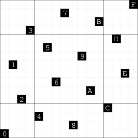
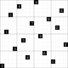
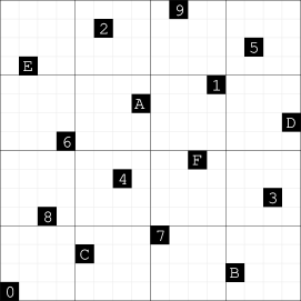
Figure 5. The first 16-point nets of 256-point (a) Hammersley (b) LP (c) Gray sequences, with possible indexings (in hexadecimal) of the points.

4. Synthetic Sequences

In this section, we demonstrate examples of applying the knowledge gained through Section 3 to synthesizing dyadic sequences with favorable properties, and in the following section we give a third demonstration of a whole class of sequences.

4.1. Designing Dyadic Nets and Sequences by Search and Optimization

For applications of Monte Carlo integration, such as rendering, one often searches for digital dyadic nets and sequences that are optimal in a sense. Common optimization targets include minimum distance between points and star discrepancy (Keller, 2006). Star discrepancy Dsuperscript𝐷D^{*} measures how the fraction n(x,y)/2m𝑛𝑥𝑦superscript2𝑚n(x,y)/2^{m} of points of an m𝑚m-net in a rectangle [0,x)×[0,y)0𝑥0𝑦[0,x)\times[0,y) deviates from the area of the rectangle; formally, D=sup|xyn(x,y)/2m|superscript𝐷supremum𝑥𝑦𝑛𝑥𝑦superscript2𝑚D^{*}=\sup|xy-n(x,y)/2^{m}|, where the supremum is over all x,y𝑥𝑦x,y in [0,1]01[0,1]. There are multiple simple ways to search for dyadic nets and sequences with specific properties. For example, for a small bit depth (m=4,N=16formulae-sequence𝑚4𝑁16m=4,N=16), it is feasible to perform an exhaustive search over all digital dyadic nets or sequences. For larger bit depths, one can use heuristic search, e.g. hill climbing. At each iteration, all possible one bit mutations to an existing net or sequence can be evaluated and the optimum mutation can be chosen until no mutation brings an improvement in the objective. One interesting possibility is a hierarchical search. Due to the incremental nature of nets and sequences we may optimize progressively, e.g. first searching for a k𝑘k bit solution and then optimizing for additional bits while retaining the leading samples (bits) in the net or sequence.

The important aspect of our work is that any of these explorations can be done efficiently. The complete characterization of the design space for nets and sequences enables us to only visit candidates, e.g. generator matrices for a digital construction, that are viable. This improves over previous work that explored a much larger set of constructions and then filtered out invalid candidates. E.g. Grünschloß et al. (2008) use heuristic search for alternative Cxsubscript𝐶𝑥C_{x} matrices to produce Hammersley-like nets. Since the percentage of viable candidates can be small, a search using our explicit construction can bring orders of magnitude speed-up.

Instead of searching for, e.g. new pairs (Cx,Cy)subscript𝐶𝑥subscript𝐶𝑦(C_{x},C_{y}), different dyadic nets are typically derived from these, especially Sobol, by applying the dyadic-preserving Owen’s scrambling (1998). Faithful application of Owen’s scrambling is computationally challenging, and common implementations offer different trade-offs between speed, quality, and flexibility (Helmer et al., 2021; Kollig and Keller, 2002; Burley, 2020). Our explicit characterization and understanding of sequences provide multiple advantages. It is hard to predict the properties of an Owen scrambled sequence. The above-mentioned hierarchical search would not be possible. Also, there are advantages when creating nets from sequences and distributing them over pixels, see e.g. PBRT (Pharr et al., 2016) or Ahmed and Wonka (2020). In Fig. 1, we show example digital dyadic sequences.

4.2. Hammersley Sequences

A Hammersley net is generated by a pair of matrices (J,I)𝐽𝐼({J},{I}). Executing Algorithm 1 by manual computation, we arrive at the progressive pair of matrices (JPJ,PJ)𝐽𝑃𝐽𝑃𝐽({J}{P}{J},{P}{J}). For example, the 256-point Hammersley net can be sequenced using the matrix pair

(10) ((1000000011000000101000001111000010001000110011001010101011111111),(1111111110101010110011001000100011110000101000001100000010000000)).10000000missing-subexpressionmissing-subexpressionmissing-subexpression11000000missing-subexpressionmissing-subexpressionmissing-subexpression10100000missing-subexpressionmissing-subexpressionmissing-subexpression11110000missing-subexpressionmissing-subexpressionmissing-subexpression10001000missing-subexpressionmissing-subexpressionmissing-subexpression11001100missing-subexpressionmissing-subexpressionmissing-subexpression10101010missing-subexpressionmissing-subexpressionmissing-subexpression11111111missing-subexpressionmissing-subexpressionmissing-subexpression11111111missing-subexpressionmissing-subexpressionmissing-subexpression10101010missing-subexpressionmissing-subexpressionmissing-subexpression11001100missing-subexpressionmissing-subexpressionmissing-subexpression10001000missing-subexpressionmissing-subexpressionmissing-subexpression11110000missing-subexpressionmissing-subexpressionmissing-subexpression10100000missing-subexpressionmissing-subexpressionmissing-subexpression11000000missing-subexpressionmissing-subexpressionmissing-subexpression10000000missing-subexpressionmissing-subexpressionmissing-subexpression\scalebox{0.8}{\mbox{$\displaystyle\left(\left(\begin{array}[]{ccccccccccc}1&\color[rgb]{.75,.75,.75}\definecolor[named]{pgfstrokecolor}{rgb}{.75,.75,.75}\pgfsys@color@gray@stroke{.75}\pgfsys@color@gray@fill{.75}0&\color[rgb]{.75,.75,.75}\definecolor[named]{pgfstrokecolor}{rgb}{.75,.75,.75}\pgfsys@color@gray@stroke{.75}\pgfsys@color@gray@fill{.75}0&\color[rgb]{.75,.75,.75}\definecolor[named]{pgfstrokecolor}{rgb}{.75,.75,.75}\pgfsys@color@gray@stroke{.75}\pgfsys@color@gray@fill{.75}0&\color[rgb]{.75,.75,.75}\definecolor[named]{pgfstrokecolor}{rgb}{.75,.75,.75}\pgfsys@color@gray@stroke{.75}\pgfsys@color@gray@fill{.75}0&\color[rgb]{.75,.75,.75}\definecolor[named]{pgfstrokecolor}{rgb}{.75,.75,.75}\pgfsys@color@gray@stroke{.75}\pgfsys@color@gray@fill{.75}0&\color[rgb]{.75,.75,.75}\definecolor[named]{pgfstrokecolor}{rgb}{.75,.75,.75}\pgfsys@color@gray@stroke{.75}\pgfsys@color@gray@fill{.75}0&\color[rgb]{.75,.75,.75}\definecolor[named]{pgfstrokecolor}{rgb}{.75,.75,.75}\pgfsys@color@gray@stroke{.75}\pgfsys@color@gray@fill{.75}0\\ 1&1&\color[rgb]{.75,.75,.75}\definecolor[named]{pgfstrokecolor}{rgb}{.75,.75,.75}\pgfsys@color@gray@stroke{.75}\pgfsys@color@gray@fill{.75}0&\color[rgb]{.75,.75,.75}\definecolor[named]{pgfstrokecolor}{rgb}{.75,.75,.75}\pgfsys@color@gray@stroke{.75}\pgfsys@color@gray@fill{.75}0&\color[rgb]{.75,.75,.75}\definecolor[named]{pgfstrokecolor}{rgb}{.75,.75,.75}\pgfsys@color@gray@stroke{.75}\pgfsys@color@gray@fill{.75}0&\color[rgb]{.75,.75,.75}\definecolor[named]{pgfstrokecolor}{rgb}{.75,.75,.75}\pgfsys@color@gray@stroke{.75}\pgfsys@color@gray@fill{.75}0&\color[rgb]{.75,.75,.75}\definecolor[named]{pgfstrokecolor}{rgb}{.75,.75,.75}\pgfsys@color@gray@stroke{.75}\pgfsys@color@gray@fill{.75}0&\color[rgb]{.75,.75,.75}\definecolor[named]{pgfstrokecolor}{rgb}{.75,.75,.75}\pgfsys@color@gray@stroke{.75}\pgfsys@color@gray@fill{.75}0\\ 1&\color[rgb]{.75,.75,.75}\definecolor[named]{pgfstrokecolor}{rgb}{.75,.75,.75}\pgfsys@color@gray@stroke{.75}\pgfsys@color@gray@fill{.75}0&1&\color[rgb]{.75,.75,.75}\definecolor[named]{pgfstrokecolor}{rgb}{.75,.75,.75}\pgfsys@color@gray@stroke{.75}\pgfsys@color@gray@fill{.75}0&\color[rgb]{.75,.75,.75}\definecolor[named]{pgfstrokecolor}{rgb}{.75,.75,.75}\pgfsys@color@gray@stroke{.75}\pgfsys@color@gray@fill{.75}0&\color[rgb]{.75,.75,.75}\definecolor[named]{pgfstrokecolor}{rgb}{.75,.75,.75}\pgfsys@color@gray@stroke{.75}\pgfsys@color@gray@fill{.75}0&\color[rgb]{.75,.75,.75}\definecolor[named]{pgfstrokecolor}{rgb}{.75,.75,.75}\pgfsys@color@gray@stroke{.75}\pgfsys@color@gray@fill{.75}0&\color[rgb]{.75,.75,.75}\definecolor[named]{pgfstrokecolor}{rgb}{.75,.75,.75}\pgfsys@color@gray@stroke{.75}\pgfsys@color@gray@fill{.75}0\\ 1&1&1&1&\color[rgb]{.75,.75,.75}\definecolor[named]{pgfstrokecolor}{rgb}{.75,.75,.75}\pgfsys@color@gray@stroke{.75}\pgfsys@color@gray@fill{.75}0&\color[rgb]{.75,.75,.75}\definecolor[named]{pgfstrokecolor}{rgb}{.75,.75,.75}\pgfsys@color@gray@stroke{.75}\pgfsys@color@gray@fill{.75}0&\color[rgb]{.75,.75,.75}\definecolor[named]{pgfstrokecolor}{rgb}{.75,.75,.75}\pgfsys@color@gray@stroke{.75}\pgfsys@color@gray@fill{.75}0&\color[rgb]{.75,.75,.75}\definecolor[named]{pgfstrokecolor}{rgb}{.75,.75,.75}\pgfsys@color@gray@stroke{.75}\pgfsys@color@gray@fill{.75}0\\ 1&\color[rgb]{.75,.75,.75}\definecolor[named]{pgfstrokecolor}{rgb}{.75,.75,.75}\pgfsys@color@gray@stroke{.75}\pgfsys@color@gray@fill{.75}0&\color[rgb]{.75,.75,.75}\definecolor[named]{pgfstrokecolor}{rgb}{.75,.75,.75}\pgfsys@color@gray@stroke{.75}\pgfsys@color@gray@fill{.75}0&\color[rgb]{.75,.75,.75}\definecolor[named]{pgfstrokecolor}{rgb}{.75,.75,.75}\pgfsys@color@gray@stroke{.75}\pgfsys@color@gray@fill{.75}0&1&\color[rgb]{.75,.75,.75}\definecolor[named]{pgfstrokecolor}{rgb}{.75,.75,.75}\pgfsys@color@gray@stroke{.75}\pgfsys@color@gray@fill{.75}0&\color[rgb]{.75,.75,.75}\definecolor[named]{pgfstrokecolor}{rgb}{.75,.75,.75}\pgfsys@color@gray@stroke{.75}\pgfsys@color@gray@fill{.75}0&\color[rgb]{.75,.75,.75}\definecolor[named]{pgfstrokecolor}{rgb}{.75,.75,.75}\pgfsys@color@gray@stroke{.75}\pgfsys@color@gray@fill{.75}0\\ 1&1&\color[rgb]{.75,.75,.75}\definecolor[named]{pgfstrokecolor}{rgb}{.75,.75,.75}\pgfsys@color@gray@stroke{.75}\pgfsys@color@gray@fill{.75}0&\color[rgb]{.75,.75,.75}\definecolor[named]{pgfstrokecolor}{rgb}{.75,.75,.75}\pgfsys@color@gray@stroke{.75}\pgfsys@color@gray@fill{.75}0&1&1&\color[rgb]{.75,.75,.75}\definecolor[named]{pgfstrokecolor}{rgb}{.75,.75,.75}\pgfsys@color@gray@stroke{.75}\pgfsys@color@gray@fill{.75}0&\color[rgb]{.75,.75,.75}\definecolor[named]{pgfstrokecolor}{rgb}{.75,.75,.75}\pgfsys@color@gray@stroke{.75}\pgfsys@color@gray@fill{.75}0\\ 1&\color[rgb]{.75,.75,.75}\definecolor[named]{pgfstrokecolor}{rgb}{.75,.75,.75}\pgfsys@color@gray@stroke{.75}\pgfsys@color@gray@fill{.75}0&1&\color[rgb]{.75,.75,.75}\definecolor[named]{pgfstrokecolor}{rgb}{.75,.75,.75}\pgfsys@color@gray@stroke{.75}\pgfsys@color@gray@fill{.75}0&1&\color[rgb]{.75,.75,.75}\definecolor[named]{pgfstrokecolor}{rgb}{.75,.75,.75}\pgfsys@color@gray@stroke{.75}\pgfsys@color@gray@fill{.75}0&1&\color[rgb]{.75,.75,.75}\definecolor[named]{pgfstrokecolor}{rgb}{.75,.75,.75}\pgfsys@color@gray@stroke{.75}\pgfsys@color@gray@fill{.75}0\\ 1&1&1&1&1&1&1&1\\ \end{array}\right),\left(\begin{array}[]{ccccccccccc}1&1&1&1&1&1&1&1\\ 1&\color[rgb]{.75,.75,.75}\definecolor[named]{pgfstrokecolor}{rgb}{.75,.75,.75}\pgfsys@color@gray@stroke{.75}\pgfsys@color@gray@fill{.75}0&1&\color[rgb]{.75,.75,.75}\definecolor[named]{pgfstrokecolor}{rgb}{.75,.75,.75}\pgfsys@color@gray@stroke{.75}\pgfsys@color@gray@fill{.75}0&1&\color[rgb]{.75,.75,.75}\definecolor[named]{pgfstrokecolor}{rgb}{.75,.75,.75}\pgfsys@color@gray@stroke{.75}\pgfsys@color@gray@fill{.75}0&1&\color[rgb]{.75,.75,.75}\definecolor[named]{pgfstrokecolor}{rgb}{.75,.75,.75}\pgfsys@color@gray@stroke{.75}\pgfsys@color@gray@fill{.75}0\\ 1&1&\color[rgb]{.75,.75,.75}\definecolor[named]{pgfstrokecolor}{rgb}{.75,.75,.75}\pgfsys@color@gray@stroke{.75}\pgfsys@color@gray@fill{.75}0&\color[rgb]{.75,.75,.75}\definecolor[named]{pgfstrokecolor}{rgb}{.75,.75,.75}\pgfsys@color@gray@stroke{.75}\pgfsys@color@gray@fill{.75}0&1&1&\color[rgb]{.75,.75,.75}\definecolor[named]{pgfstrokecolor}{rgb}{.75,.75,.75}\pgfsys@color@gray@stroke{.75}\pgfsys@color@gray@fill{.75}0&\color[rgb]{.75,.75,.75}\definecolor[named]{pgfstrokecolor}{rgb}{.75,.75,.75}\pgfsys@color@gray@stroke{.75}\pgfsys@color@gray@fill{.75}0\\ 1&\color[rgb]{.75,.75,.75}\definecolor[named]{pgfstrokecolor}{rgb}{.75,.75,.75}\pgfsys@color@gray@stroke{.75}\pgfsys@color@gray@fill{.75}0&\color[rgb]{.75,.75,.75}\definecolor[named]{pgfstrokecolor}{rgb}{.75,.75,.75}\pgfsys@color@gray@stroke{.75}\pgfsys@color@gray@fill{.75}0&\color[rgb]{.75,.75,.75}\definecolor[named]{pgfstrokecolor}{rgb}{.75,.75,.75}\pgfsys@color@gray@stroke{.75}\pgfsys@color@gray@fill{.75}0&1&\color[rgb]{.75,.75,.75}\definecolor[named]{pgfstrokecolor}{rgb}{.75,.75,.75}\pgfsys@color@gray@stroke{.75}\pgfsys@color@gray@fill{.75}0&\color[rgb]{.75,.75,.75}\definecolor[named]{pgfstrokecolor}{rgb}{.75,.75,.75}\pgfsys@color@gray@stroke{.75}\pgfsys@color@gray@fill{.75}0&\color[rgb]{.75,.75,.75}\definecolor[named]{pgfstrokecolor}{rgb}{.75,.75,.75}\pgfsys@color@gray@stroke{.75}\pgfsys@color@gray@fill{.75}0\\ 1&1&1&1&\color[rgb]{.75,.75,.75}\definecolor[named]{pgfstrokecolor}{rgb}{.75,.75,.75}\pgfsys@color@gray@stroke{.75}\pgfsys@color@gray@fill{.75}0&\color[rgb]{.75,.75,.75}\definecolor[named]{pgfstrokecolor}{rgb}{.75,.75,.75}\pgfsys@color@gray@stroke{.75}\pgfsys@color@gray@fill{.75}0&\color[rgb]{.75,.75,.75}\definecolor[named]{pgfstrokecolor}{rgb}{.75,.75,.75}\pgfsys@color@gray@stroke{.75}\pgfsys@color@gray@fill{.75}0&\color[rgb]{.75,.75,.75}\definecolor[named]{pgfstrokecolor}{rgb}{.75,.75,.75}\pgfsys@color@gray@stroke{.75}\pgfsys@color@gray@fill{.75}0\\ 1&\color[rgb]{.75,.75,.75}\definecolor[named]{pgfstrokecolor}{rgb}{.75,.75,.75}\pgfsys@color@gray@stroke{.75}\pgfsys@color@gray@fill{.75}0&1&\color[rgb]{.75,.75,.75}\definecolor[named]{pgfstrokecolor}{rgb}{.75,.75,.75}\pgfsys@color@gray@stroke{.75}\pgfsys@color@gray@fill{.75}0&\color[rgb]{.75,.75,.75}\definecolor[named]{pgfstrokecolor}{rgb}{.75,.75,.75}\pgfsys@color@gray@stroke{.75}\pgfsys@color@gray@fill{.75}0&\color[rgb]{.75,.75,.75}\definecolor[named]{pgfstrokecolor}{rgb}{.75,.75,.75}\pgfsys@color@gray@stroke{.75}\pgfsys@color@gray@fill{.75}0&\color[rgb]{.75,.75,.75}\definecolor[named]{pgfstrokecolor}{rgb}{.75,.75,.75}\pgfsys@color@gray@stroke{.75}\pgfsys@color@gray@fill{.75}0&\color[rgb]{.75,.75,.75}\definecolor[named]{pgfstrokecolor}{rgb}{.75,.75,.75}\pgfsys@color@gray@stroke{.75}\pgfsys@color@gray@fill{.75}0\\ 1&1&\color[rgb]{.75,.75,.75}\definecolor[named]{pgfstrokecolor}{rgb}{.75,.75,.75}\pgfsys@color@gray@stroke{.75}\pgfsys@color@gray@fill{.75}0&\color[rgb]{.75,.75,.75}\definecolor[named]{pgfstrokecolor}{rgb}{.75,.75,.75}\pgfsys@color@gray@stroke{.75}\pgfsys@color@gray@fill{.75}0&\color[rgb]{.75,.75,.75}\definecolor[named]{pgfstrokecolor}{rgb}{.75,.75,.75}\pgfsys@color@gray@stroke{.75}\pgfsys@color@gray@fill{.75}0&\color[rgb]{.75,.75,.75}\definecolor[named]{pgfstrokecolor}{rgb}{.75,.75,.75}\pgfsys@color@gray@stroke{.75}\pgfsys@color@gray@fill{.75}0&\color[rgb]{.75,.75,.75}\definecolor[named]{pgfstrokecolor}{rgb}{.75,.75,.75}\pgfsys@color@gray@stroke{.75}\pgfsys@color@gray@fill{.75}0&\color[rgb]{.75,.75,.75}\definecolor[named]{pgfstrokecolor}{rgb}{.75,.75,.75}\pgfsys@color@gray@stroke{.75}\pgfsys@color@gray@fill{.75}0\\ 1&\color[rgb]{.75,.75,.75}\definecolor[named]{pgfstrokecolor}{rgb}{.75,.75,.75}\pgfsys@color@gray@stroke{.75}\pgfsys@color@gray@fill{.75}0&\color[rgb]{.75,.75,.75}\definecolor[named]{pgfstrokecolor}{rgb}{.75,.75,.75}\pgfsys@color@gray@stroke{.75}\pgfsys@color@gray@fill{.75}0&\color[rgb]{.75,.75,.75}\definecolor[named]{pgfstrokecolor}{rgb}{.75,.75,.75}\pgfsys@color@gray@stroke{.75}\pgfsys@color@gray@fill{.75}0&\color[rgb]{.75,.75,.75}\definecolor[named]{pgfstrokecolor}{rgb}{.75,.75,.75}\pgfsys@color@gray@stroke{.75}\pgfsys@color@gray@fill{.75}0&\color[rgb]{.75,.75,.75}\definecolor[named]{pgfstrokecolor}{rgb}{.75,.75,.75}\pgfsys@color@gray@stroke{.75}\pgfsys@color@gray@fill{.75}0&\color[rgb]{.75,.75,.75}\definecolor[named]{pgfstrokecolor}{rgb}{.75,.75,.75}\pgfsys@color@gray@stroke{.75}\pgfsys@color@gray@fill{.75}0&\color[rgb]{.75,.75,.75}\definecolor[named]{pgfstrokecolor}{rgb}{.75,.75,.75}\pgfsys@color@gray@stroke{.75}\pgfsys@color@gray@fill{.75}0\\ \end{array}\right)\right)$}}\,.

See Fig. 5(a) for the layout of the first 16-point net in the 256-point sequence with possible indexing.

4.3. LP Sequences

While the Hammersley nets have the worst known star discrepancy among digital dyadic nets, the LP nets of Larcher and Pillichshammer (2003) are believed to have the best one according to numerical experiments measuring the star discrepancy. We use 22ksuperscript2superscript2𝑘2^{2^{k}}-point LP nets as a second example of converting a net into a sequence.

An LP net is generated by the pair of matrices (J,ULP)𝐽subscript𝑈LP(J,U_{\mathrm{LP}}) given by (3). The corresponding sequence is generated by the pair (LLP,PJ)subscript𝐿LP𝑃𝐽(L_{\mathrm{LP}},PJ), where LLP=Lsubscript𝐿LP𝐿L_{\mathrm{LP}}=L is the lower-unitriangular matrix with the entries

(11) L11=1,Li1=L1j=0,Lij=(i2j2)mod2 for 2i,jm.formulae-sequenceformulae-sequencesubscript𝐿111subscript𝐿𝑖1subscript𝐿1𝑗0formulae-sequencesubscript𝐿𝑖𝑗modulobinomial𝑖2𝑗22formulae-sequence for 2𝑖𝑗𝑚L_{11}=1,L_{i1}=L_{1j}=0,L_{ij}=\binom{i-2}{j-2}\mod 2\quad\text{ for }2\leq i,j\leq m.

Indeed, the pair (LLP,PJ)subscript𝐿LP𝑃𝐽(L_{\mathrm{LP}},PJ) is progressive by Theorem 3.9 because PJ=JPJP=:LyPPJ=JPJ\cdot P=:L_{y}\cdot P. The pair (LLP,PJ)subscript𝐿LP𝑃𝐽(L_{\mathrm{LP}},PJ) generates the same net because the characteristic matrices are the same: PJLLP1=ULPJ𝑃𝐽subscriptsuperscript𝐿1LPsubscript𝑈LP𝐽PJL^{-1}_{\mathrm{LP}}=U_{\mathrm{LP}}J if m𝑚m is a power of 222. This identity is proved at the end of Appendix B. For example, the following pair of matrices creates a 256-point LP net as a digital dyadic sequence:

(12) ((1000000001000000011000000101000001111000010001000110011001010101),(1111111110101010110011001000100011110000101000001100000010000000)).10000000missing-subexpressionmissing-subexpressionmissing-subexpression01000000missing-subexpressionmissing-subexpressionmissing-subexpression01100000missing-subexpressionmissing-subexpressionmissing-subexpression01010000missing-subexpressionmissing-subexpressionmissing-subexpression01111000missing-subexpressionmissing-subexpressionmissing-subexpression01000100missing-subexpressionmissing-subexpressionmissing-subexpression01100110missing-subexpressionmissing-subexpressionmissing-subexpression01010101missing-subexpressionmissing-subexpressionmissing-subexpression11111111missing-subexpressionmissing-subexpressionmissing-subexpression10101010missing-subexpressionmissing-subexpressionmissing-subexpression11001100missing-subexpressionmissing-subexpressionmissing-subexpression10001000missing-subexpressionmissing-subexpressionmissing-subexpression11110000missing-subexpressionmissing-subexpressionmissing-subexpression10100000missing-subexpressionmissing-subexpressionmissing-subexpression11000000missing-subexpressionmissing-subexpressionmissing-subexpression10000000missing-subexpressionmissing-subexpressionmissing-subexpression\scalebox{0.8}{\mbox{$\displaystyle\left(\left(\begin{array}[]{ccccccccccc}1&\color[rgb]{.75,.75,.75}\definecolor[named]{pgfstrokecolor}{rgb}{.75,.75,.75}\pgfsys@color@gray@stroke{.75}\pgfsys@color@gray@fill{.75}0&\color[rgb]{.75,.75,.75}\definecolor[named]{pgfstrokecolor}{rgb}{.75,.75,.75}\pgfsys@color@gray@stroke{.75}\pgfsys@color@gray@fill{.75}0&\color[rgb]{.75,.75,.75}\definecolor[named]{pgfstrokecolor}{rgb}{.75,.75,.75}\pgfsys@color@gray@stroke{.75}\pgfsys@color@gray@fill{.75}0&\color[rgb]{.75,.75,.75}\definecolor[named]{pgfstrokecolor}{rgb}{.75,.75,.75}\pgfsys@color@gray@stroke{.75}\pgfsys@color@gray@fill{.75}0&\color[rgb]{.75,.75,.75}\definecolor[named]{pgfstrokecolor}{rgb}{.75,.75,.75}\pgfsys@color@gray@stroke{.75}\pgfsys@color@gray@fill{.75}0&\color[rgb]{.75,.75,.75}\definecolor[named]{pgfstrokecolor}{rgb}{.75,.75,.75}\pgfsys@color@gray@stroke{.75}\pgfsys@color@gray@fill{.75}0&\color[rgb]{.75,.75,.75}\definecolor[named]{pgfstrokecolor}{rgb}{.75,.75,.75}\pgfsys@color@gray@stroke{.75}\pgfsys@color@gray@fill{.75}0\\ \color[rgb]{.75,.75,.75}\definecolor[named]{pgfstrokecolor}{rgb}{.75,.75,.75}\pgfsys@color@gray@stroke{.75}\pgfsys@color@gray@fill{.75}0&1&\color[rgb]{.75,.75,.75}\definecolor[named]{pgfstrokecolor}{rgb}{.75,.75,.75}\pgfsys@color@gray@stroke{.75}\pgfsys@color@gray@fill{.75}0&\color[rgb]{.75,.75,.75}\definecolor[named]{pgfstrokecolor}{rgb}{.75,.75,.75}\pgfsys@color@gray@stroke{.75}\pgfsys@color@gray@fill{.75}0&\color[rgb]{.75,.75,.75}\definecolor[named]{pgfstrokecolor}{rgb}{.75,.75,.75}\pgfsys@color@gray@stroke{.75}\pgfsys@color@gray@fill{.75}0&\color[rgb]{.75,.75,.75}\definecolor[named]{pgfstrokecolor}{rgb}{.75,.75,.75}\pgfsys@color@gray@stroke{.75}\pgfsys@color@gray@fill{.75}0&\color[rgb]{.75,.75,.75}\definecolor[named]{pgfstrokecolor}{rgb}{.75,.75,.75}\pgfsys@color@gray@stroke{.75}\pgfsys@color@gray@fill{.75}0&\color[rgb]{.75,.75,.75}\definecolor[named]{pgfstrokecolor}{rgb}{.75,.75,.75}\pgfsys@color@gray@stroke{.75}\pgfsys@color@gray@fill{.75}0\\ \color[rgb]{.75,.75,.75}\definecolor[named]{pgfstrokecolor}{rgb}{.75,.75,.75}\pgfsys@color@gray@stroke{.75}\pgfsys@color@gray@fill{.75}0&1&1&\color[rgb]{.75,.75,.75}\definecolor[named]{pgfstrokecolor}{rgb}{.75,.75,.75}\pgfsys@color@gray@stroke{.75}\pgfsys@color@gray@fill{.75}0&\color[rgb]{.75,.75,.75}\definecolor[named]{pgfstrokecolor}{rgb}{.75,.75,.75}\pgfsys@color@gray@stroke{.75}\pgfsys@color@gray@fill{.75}0&\color[rgb]{.75,.75,.75}\definecolor[named]{pgfstrokecolor}{rgb}{.75,.75,.75}\pgfsys@color@gray@stroke{.75}\pgfsys@color@gray@fill{.75}0&\color[rgb]{.75,.75,.75}\definecolor[named]{pgfstrokecolor}{rgb}{.75,.75,.75}\pgfsys@color@gray@stroke{.75}\pgfsys@color@gray@fill{.75}0&\color[rgb]{.75,.75,.75}\definecolor[named]{pgfstrokecolor}{rgb}{.75,.75,.75}\pgfsys@color@gray@stroke{.75}\pgfsys@color@gray@fill{.75}0\\ \color[rgb]{.75,.75,.75}\definecolor[named]{pgfstrokecolor}{rgb}{.75,.75,.75}\pgfsys@color@gray@stroke{.75}\pgfsys@color@gray@fill{.75}0&1&\color[rgb]{.75,.75,.75}\definecolor[named]{pgfstrokecolor}{rgb}{.75,.75,.75}\pgfsys@color@gray@stroke{.75}\pgfsys@color@gray@fill{.75}0&1&\color[rgb]{.75,.75,.75}\definecolor[named]{pgfstrokecolor}{rgb}{.75,.75,.75}\pgfsys@color@gray@stroke{.75}\pgfsys@color@gray@fill{.75}0&\color[rgb]{.75,.75,.75}\definecolor[named]{pgfstrokecolor}{rgb}{.75,.75,.75}\pgfsys@color@gray@stroke{.75}\pgfsys@color@gray@fill{.75}0&\color[rgb]{.75,.75,.75}\definecolor[named]{pgfstrokecolor}{rgb}{.75,.75,.75}\pgfsys@color@gray@stroke{.75}\pgfsys@color@gray@fill{.75}0&\color[rgb]{.75,.75,.75}\definecolor[named]{pgfstrokecolor}{rgb}{.75,.75,.75}\pgfsys@color@gray@stroke{.75}\pgfsys@color@gray@fill{.75}0\\ \color[rgb]{.75,.75,.75}\definecolor[named]{pgfstrokecolor}{rgb}{.75,.75,.75}\pgfsys@color@gray@stroke{.75}\pgfsys@color@gray@fill{.75}0&1&1&1&1&\color[rgb]{.75,.75,.75}\definecolor[named]{pgfstrokecolor}{rgb}{.75,.75,.75}\pgfsys@color@gray@stroke{.75}\pgfsys@color@gray@fill{.75}0&\color[rgb]{.75,.75,.75}\definecolor[named]{pgfstrokecolor}{rgb}{.75,.75,.75}\pgfsys@color@gray@stroke{.75}\pgfsys@color@gray@fill{.75}0&\color[rgb]{.75,.75,.75}\definecolor[named]{pgfstrokecolor}{rgb}{.75,.75,.75}\pgfsys@color@gray@stroke{.75}\pgfsys@color@gray@fill{.75}0\\ \color[rgb]{.75,.75,.75}\definecolor[named]{pgfstrokecolor}{rgb}{.75,.75,.75}\pgfsys@color@gray@stroke{.75}\pgfsys@color@gray@fill{.75}0&1&\color[rgb]{.75,.75,.75}\definecolor[named]{pgfstrokecolor}{rgb}{.75,.75,.75}\pgfsys@color@gray@stroke{.75}\pgfsys@color@gray@fill{.75}0&\color[rgb]{.75,.75,.75}\definecolor[named]{pgfstrokecolor}{rgb}{.75,.75,.75}\pgfsys@color@gray@stroke{.75}\pgfsys@color@gray@fill{.75}0&\color[rgb]{.75,.75,.75}\definecolor[named]{pgfstrokecolor}{rgb}{.75,.75,.75}\pgfsys@color@gray@stroke{.75}\pgfsys@color@gray@fill{.75}0&1&\color[rgb]{.75,.75,.75}\definecolor[named]{pgfstrokecolor}{rgb}{.75,.75,.75}\pgfsys@color@gray@stroke{.75}\pgfsys@color@gray@fill{.75}0&\color[rgb]{.75,.75,.75}\definecolor[named]{pgfstrokecolor}{rgb}{.75,.75,.75}\pgfsys@color@gray@stroke{.75}\pgfsys@color@gray@fill{.75}0\\ \color[rgb]{.75,.75,.75}\definecolor[named]{pgfstrokecolor}{rgb}{.75,.75,.75}\pgfsys@color@gray@stroke{.75}\pgfsys@color@gray@fill{.75}0&1&1&\color[rgb]{.75,.75,.75}\definecolor[named]{pgfstrokecolor}{rgb}{.75,.75,.75}\pgfsys@color@gray@stroke{.75}\pgfsys@color@gray@fill{.75}0&\color[rgb]{.75,.75,.75}\definecolor[named]{pgfstrokecolor}{rgb}{.75,.75,.75}\pgfsys@color@gray@stroke{.75}\pgfsys@color@gray@fill{.75}0&1&1&\color[rgb]{.75,.75,.75}\definecolor[named]{pgfstrokecolor}{rgb}{.75,.75,.75}\pgfsys@color@gray@stroke{.75}\pgfsys@color@gray@fill{.75}0\\ \color[rgb]{.75,.75,.75}\definecolor[named]{pgfstrokecolor}{rgb}{.75,.75,.75}\pgfsys@color@gray@stroke{.75}\pgfsys@color@gray@fill{.75}0&1&\color[rgb]{.75,.75,.75}\definecolor[named]{pgfstrokecolor}{rgb}{.75,.75,.75}\pgfsys@color@gray@stroke{.75}\pgfsys@color@gray@fill{.75}0&1&\color[rgb]{.75,.75,.75}\definecolor[named]{pgfstrokecolor}{rgb}{.75,.75,.75}\pgfsys@color@gray@stroke{.75}\pgfsys@color@gray@fill{.75}0&1&\color[rgb]{.75,.75,.75}\definecolor[named]{pgfstrokecolor}{rgb}{.75,.75,.75}\pgfsys@color@gray@stroke{.75}\pgfsys@color@gray@fill{.75}0&1\\ \end{array}\right),\left(\begin{array}[]{ccccccccccc}1&1&1&1&1&1&1&1\\ 1&\color[rgb]{.75,.75,.75}\definecolor[named]{pgfstrokecolor}{rgb}{.75,.75,.75}\pgfsys@color@gray@stroke{.75}\pgfsys@color@gray@fill{.75}0&1&\color[rgb]{.75,.75,.75}\definecolor[named]{pgfstrokecolor}{rgb}{.75,.75,.75}\pgfsys@color@gray@stroke{.75}\pgfsys@color@gray@fill{.75}0&1&\color[rgb]{.75,.75,.75}\definecolor[named]{pgfstrokecolor}{rgb}{.75,.75,.75}\pgfsys@color@gray@stroke{.75}\pgfsys@color@gray@fill{.75}0&1&\color[rgb]{.75,.75,.75}\definecolor[named]{pgfstrokecolor}{rgb}{.75,.75,.75}\pgfsys@color@gray@stroke{.75}\pgfsys@color@gray@fill{.75}0\\ 1&1&\color[rgb]{.75,.75,.75}\definecolor[named]{pgfstrokecolor}{rgb}{.75,.75,.75}\pgfsys@color@gray@stroke{.75}\pgfsys@color@gray@fill{.75}0&\color[rgb]{.75,.75,.75}\definecolor[named]{pgfstrokecolor}{rgb}{.75,.75,.75}\pgfsys@color@gray@stroke{.75}\pgfsys@color@gray@fill{.75}0&1&1&\color[rgb]{.75,.75,.75}\definecolor[named]{pgfstrokecolor}{rgb}{.75,.75,.75}\pgfsys@color@gray@stroke{.75}\pgfsys@color@gray@fill{.75}0&\color[rgb]{.75,.75,.75}\definecolor[named]{pgfstrokecolor}{rgb}{.75,.75,.75}\pgfsys@color@gray@stroke{.75}\pgfsys@color@gray@fill{.75}0\\ 1&\color[rgb]{.75,.75,.75}\definecolor[named]{pgfstrokecolor}{rgb}{.75,.75,.75}\pgfsys@color@gray@stroke{.75}\pgfsys@color@gray@fill{.75}0&\color[rgb]{.75,.75,.75}\definecolor[named]{pgfstrokecolor}{rgb}{.75,.75,.75}\pgfsys@color@gray@stroke{.75}\pgfsys@color@gray@fill{.75}0&\color[rgb]{.75,.75,.75}\definecolor[named]{pgfstrokecolor}{rgb}{.75,.75,.75}\pgfsys@color@gray@stroke{.75}\pgfsys@color@gray@fill{.75}0&1&\color[rgb]{.75,.75,.75}\definecolor[named]{pgfstrokecolor}{rgb}{.75,.75,.75}\pgfsys@color@gray@stroke{.75}\pgfsys@color@gray@fill{.75}0&\color[rgb]{.75,.75,.75}\definecolor[named]{pgfstrokecolor}{rgb}{.75,.75,.75}\pgfsys@color@gray@stroke{.75}\pgfsys@color@gray@fill{.75}0&\color[rgb]{.75,.75,.75}\definecolor[named]{pgfstrokecolor}{rgb}{.75,.75,.75}\pgfsys@color@gray@stroke{.75}\pgfsys@color@gray@fill{.75}0\\ 1&1&1&1&\color[rgb]{.75,.75,.75}\definecolor[named]{pgfstrokecolor}{rgb}{.75,.75,.75}\pgfsys@color@gray@stroke{.75}\pgfsys@color@gray@fill{.75}0&\color[rgb]{.75,.75,.75}\definecolor[named]{pgfstrokecolor}{rgb}{.75,.75,.75}\pgfsys@color@gray@stroke{.75}\pgfsys@color@gray@fill{.75}0&\color[rgb]{.75,.75,.75}\definecolor[named]{pgfstrokecolor}{rgb}{.75,.75,.75}\pgfsys@color@gray@stroke{.75}\pgfsys@color@gray@fill{.75}0&\color[rgb]{.75,.75,.75}\definecolor[named]{pgfstrokecolor}{rgb}{.75,.75,.75}\pgfsys@color@gray@stroke{.75}\pgfsys@color@gray@fill{.75}0\\ 1&\color[rgb]{.75,.75,.75}\definecolor[named]{pgfstrokecolor}{rgb}{.75,.75,.75}\pgfsys@color@gray@stroke{.75}\pgfsys@color@gray@fill{.75}0&1&\color[rgb]{.75,.75,.75}\definecolor[named]{pgfstrokecolor}{rgb}{.75,.75,.75}\pgfsys@color@gray@stroke{.75}\pgfsys@color@gray@fill{.75}0&\color[rgb]{.75,.75,.75}\definecolor[named]{pgfstrokecolor}{rgb}{.75,.75,.75}\pgfsys@color@gray@stroke{.75}\pgfsys@color@gray@fill{.75}0&\color[rgb]{.75,.75,.75}\definecolor[named]{pgfstrokecolor}{rgb}{.75,.75,.75}\pgfsys@color@gray@stroke{.75}\pgfsys@color@gray@fill{.75}0&\color[rgb]{.75,.75,.75}\definecolor[named]{pgfstrokecolor}{rgb}{.75,.75,.75}\pgfsys@color@gray@stroke{.75}\pgfsys@color@gray@fill{.75}0&\color[rgb]{.75,.75,.75}\definecolor[named]{pgfstrokecolor}{rgb}{.75,.75,.75}\pgfsys@color@gray@stroke{.75}\pgfsys@color@gray@fill{.75}0\\ 1&1&\color[rgb]{.75,.75,.75}\definecolor[named]{pgfstrokecolor}{rgb}{.75,.75,.75}\pgfsys@color@gray@stroke{.75}\pgfsys@color@gray@fill{.75}0&\color[rgb]{.75,.75,.75}\definecolor[named]{pgfstrokecolor}{rgb}{.75,.75,.75}\pgfsys@color@gray@stroke{.75}\pgfsys@color@gray@fill{.75}0&\color[rgb]{.75,.75,.75}\definecolor[named]{pgfstrokecolor}{rgb}{.75,.75,.75}\pgfsys@color@gray@stroke{.75}\pgfsys@color@gray@fill{.75}0&\color[rgb]{.75,.75,.75}\definecolor[named]{pgfstrokecolor}{rgb}{.75,.75,.75}\pgfsys@color@gray@stroke{.75}\pgfsys@color@gray@fill{.75}0&\color[rgb]{.75,.75,.75}\definecolor[named]{pgfstrokecolor}{rgb}{.75,.75,.75}\pgfsys@color@gray@stroke{.75}\pgfsys@color@gray@fill{.75}0&\color[rgb]{.75,.75,.75}\definecolor[named]{pgfstrokecolor}{rgb}{.75,.75,.75}\pgfsys@color@gray@stroke{.75}\pgfsys@color@gray@fill{.75}0\\ 1&\color[rgb]{.75,.75,.75}\definecolor[named]{pgfstrokecolor}{rgb}{.75,.75,.75}\pgfsys@color@gray@stroke{.75}\pgfsys@color@gray@fill{.75}0&\color[rgb]{.75,.75,.75}\definecolor[named]{pgfstrokecolor}{rgb}{.75,.75,.75}\pgfsys@color@gray@stroke{.75}\pgfsys@color@gray@fill{.75}0&\color[rgb]{.75,.75,.75}\definecolor[named]{pgfstrokecolor}{rgb}{.75,.75,.75}\pgfsys@color@gray@stroke{.75}\pgfsys@color@gray@fill{.75}0&\color[rgb]{.75,.75,.75}\definecolor[named]{pgfstrokecolor}{rgb}{.75,.75,.75}\pgfsys@color@gray@stroke{.75}\pgfsys@color@gray@fill{.75}0&\color[rgb]{.75,.75,.75}\definecolor[named]{pgfstrokecolor}{rgb}{.75,.75,.75}\pgfsys@color@gray@stroke{.75}\pgfsys@color@gray@fill{.75}0&\color[rgb]{.75,.75,.75}\definecolor[named]{pgfstrokecolor}{rgb}{.75,.75,.75}\pgfsys@color@gray@stroke{.75}\pgfsys@color@gray@fill{.75}0&\color[rgb]{.75,.75,.75}\definecolor[named]{pgfstrokecolor}{rgb}{.75,.75,.75}\pgfsys@color@gray@stroke{.75}\pgfsys@color@gray@fill{.75}0\\ \end{array}\right)\right)$}}\,.

See Fig. 5(b). The analysis of the star discrepancy of all possible sub-sequences is an interesting open question.

4.4. Converting Point Sets to Digital Dyadic Sequences

Algorithm 2 can be used to test if an arbitrary set of points (including sets of points that are known dyadic nets) allows for a digital construction. If it is possible, the algorithm produces the pair of matrices that generate the given set of points as a digital dyadic sequence.

Input: an arbitrary 2msuperscript2𝑚2^{m}-point set in [0,1)2superscript012[0,1)^{2};
Output: a pair of matrices that creates a digital dyadic sequence with the same points using (1), if it exists.
1 Order the points sequentially along the x𝑥x-axis and set Cx=Jsubscript𝐶𝑥𝐽C_{x}={J};
2 Use the y𝑦y-coordinates of the points at power-of-two indices as columns of the prospected Cysubscript𝐶𝑦C_{y};
3 Conduct one pass through the other points to validate if they coincide with the ones given by (1), and check if Cysubscript𝐶𝑦C_{y} is progressive;
If this step works, we have a digital dyadic net that can subsequently be converted to a sequence using Algorithm 1.
Algorithm 2 Converting a point set into a digital dyadic sequence

4.5. Gray Sequences

We applied the conversion algorithm above to the Gray Code family of nets introduced by Ahmed and Wonka (2021), obtained by using a Gray Code-ordered van der Corput sequence to supplement the x𝑥x-offsets of the points along the columns and the y𝑦y-offsets along the rows. These nets turned out to be digital.

A 256-point Gray net (from now on, we will drop the word “Code”) is generated by the pair of matrices (J,C)𝐽superscript𝐶(J,C^{\prime}), where

(13) C=(1000000011000000111000001111000000001100000001100000001100000001).superscript𝐶10000000missing-subexpressionmissing-subexpressionmissing-subexpression11000000missing-subexpressionmissing-subexpressionmissing-subexpression11100000missing-subexpressionmissing-subexpressionmissing-subexpression11110000missing-subexpressionmissing-subexpressionmissing-subexpression00001100missing-subexpressionmissing-subexpressionmissing-subexpression00000110missing-subexpressionmissing-subexpressionmissing-subexpression00000011missing-subexpressionmissing-subexpressionmissing-subexpression00000001missing-subexpressionmissing-subexpressionmissing-subexpressionC^{\prime}=\scalebox{0.8}{\mbox{$\displaystyle\left(\begin{array}[]{ccccccccccc}1&\color[rgb]{.75,.75,.75}\definecolor[named]{pgfstrokecolor}{rgb}{.75,.75,.75}\pgfsys@color@gray@stroke{.75}\pgfsys@color@gray@fill{.75}0&\color[rgb]{.75,.75,.75}\definecolor[named]{pgfstrokecolor}{rgb}{.75,.75,.75}\pgfsys@color@gray@stroke{.75}\pgfsys@color@gray@fill{.75}0&\color[rgb]{.75,.75,.75}\definecolor[named]{pgfstrokecolor}{rgb}{.75,.75,.75}\pgfsys@color@gray@stroke{.75}\pgfsys@color@gray@fill{.75}0&\color[rgb]{.75,.75,.75}\definecolor[named]{pgfstrokecolor}{rgb}{.75,.75,.75}\pgfsys@color@gray@stroke{.75}\pgfsys@color@gray@fill{.75}0&\color[rgb]{.75,.75,.75}\definecolor[named]{pgfstrokecolor}{rgb}{.75,.75,.75}\pgfsys@color@gray@stroke{.75}\pgfsys@color@gray@fill{.75}0&\color[rgb]{.75,.75,.75}\definecolor[named]{pgfstrokecolor}{rgb}{.75,.75,.75}\pgfsys@color@gray@stroke{.75}\pgfsys@color@gray@fill{.75}0&\color[rgb]{.75,.75,.75}\definecolor[named]{pgfstrokecolor}{rgb}{.75,.75,.75}\pgfsys@color@gray@stroke{.75}\pgfsys@color@gray@fill{.75}0\\ 1&1&\color[rgb]{.75,.75,.75}\definecolor[named]{pgfstrokecolor}{rgb}{.75,.75,.75}\pgfsys@color@gray@stroke{.75}\pgfsys@color@gray@fill{.75}0&\color[rgb]{.75,.75,.75}\definecolor[named]{pgfstrokecolor}{rgb}{.75,.75,.75}\pgfsys@color@gray@stroke{.75}\pgfsys@color@gray@fill{.75}0&\color[rgb]{.75,.75,.75}\definecolor[named]{pgfstrokecolor}{rgb}{.75,.75,.75}\pgfsys@color@gray@stroke{.75}\pgfsys@color@gray@fill{.75}0&\color[rgb]{.75,.75,.75}\definecolor[named]{pgfstrokecolor}{rgb}{.75,.75,.75}\pgfsys@color@gray@stroke{.75}\pgfsys@color@gray@fill{.75}0&\color[rgb]{.75,.75,.75}\definecolor[named]{pgfstrokecolor}{rgb}{.75,.75,.75}\pgfsys@color@gray@stroke{.75}\pgfsys@color@gray@fill{.75}0&\color[rgb]{.75,.75,.75}\definecolor[named]{pgfstrokecolor}{rgb}{.75,.75,.75}\pgfsys@color@gray@stroke{.75}\pgfsys@color@gray@fill{.75}0\\ 1&1&1&\color[rgb]{.75,.75,.75}\definecolor[named]{pgfstrokecolor}{rgb}{.75,.75,.75}\pgfsys@color@gray@stroke{.75}\pgfsys@color@gray@fill{.75}0&\color[rgb]{.75,.75,.75}\definecolor[named]{pgfstrokecolor}{rgb}{.75,.75,.75}\pgfsys@color@gray@stroke{.75}\pgfsys@color@gray@fill{.75}0&\color[rgb]{.75,.75,.75}\definecolor[named]{pgfstrokecolor}{rgb}{.75,.75,.75}\pgfsys@color@gray@stroke{.75}\pgfsys@color@gray@fill{.75}0&\color[rgb]{.75,.75,.75}\definecolor[named]{pgfstrokecolor}{rgb}{.75,.75,.75}\pgfsys@color@gray@stroke{.75}\pgfsys@color@gray@fill{.75}0&\color[rgb]{.75,.75,.75}\definecolor[named]{pgfstrokecolor}{rgb}{.75,.75,.75}\pgfsys@color@gray@stroke{.75}\pgfsys@color@gray@fill{.75}0\\ 1&1&1&1&\color[rgb]{.75,.75,.75}\definecolor[named]{pgfstrokecolor}{rgb}{.75,.75,.75}\pgfsys@color@gray@stroke{.75}\pgfsys@color@gray@fill{.75}0&\color[rgb]{.75,.75,.75}\definecolor[named]{pgfstrokecolor}{rgb}{.75,.75,.75}\pgfsys@color@gray@stroke{.75}\pgfsys@color@gray@fill{.75}0&\color[rgb]{.75,.75,.75}\definecolor[named]{pgfstrokecolor}{rgb}{.75,.75,.75}\pgfsys@color@gray@stroke{.75}\pgfsys@color@gray@fill{.75}0&\color[rgb]{.75,.75,.75}\definecolor[named]{pgfstrokecolor}{rgb}{.75,.75,.75}\pgfsys@color@gray@stroke{.75}\pgfsys@color@gray@fill{.75}0\\ \color[rgb]{.75,.75,.75}\definecolor[named]{pgfstrokecolor}{rgb}{.75,.75,.75}\pgfsys@color@gray@stroke{.75}\pgfsys@color@gray@fill{.75}0&\color[rgb]{.75,.75,.75}\definecolor[named]{pgfstrokecolor}{rgb}{.75,.75,.75}\pgfsys@color@gray@stroke{.75}\pgfsys@color@gray@fill{.75}0&\color[rgb]{.75,.75,.75}\definecolor[named]{pgfstrokecolor}{rgb}{.75,.75,.75}\pgfsys@color@gray@stroke{.75}\pgfsys@color@gray@fill{.75}0&\color[rgb]{.75,.75,.75}\definecolor[named]{pgfstrokecolor}{rgb}{.75,.75,.75}\pgfsys@color@gray@stroke{.75}\pgfsys@color@gray@fill{.75}0&1&1&\color[rgb]{.75,.75,.75}\definecolor[named]{pgfstrokecolor}{rgb}{.75,.75,.75}\pgfsys@color@gray@stroke{.75}\pgfsys@color@gray@fill{.75}0&\color[rgb]{.75,.75,.75}\definecolor[named]{pgfstrokecolor}{rgb}{.75,.75,.75}\pgfsys@color@gray@stroke{.75}\pgfsys@color@gray@fill{.75}0\\ \color[rgb]{.75,.75,.75}\definecolor[named]{pgfstrokecolor}{rgb}{.75,.75,.75}\pgfsys@color@gray@stroke{.75}\pgfsys@color@gray@fill{.75}0&\color[rgb]{.75,.75,.75}\definecolor[named]{pgfstrokecolor}{rgb}{.75,.75,.75}\pgfsys@color@gray@stroke{.75}\pgfsys@color@gray@fill{.75}0&\color[rgb]{.75,.75,.75}\definecolor[named]{pgfstrokecolor}{rgb}{.75,.75,.75}\pgfsys@color@gray@stroke{.75}\pgfsys@color@gray@fill{.75}0&\color[rgb]{.75,.75,.75}\definecolor[named]{pgfstrokecolor}{rgb}{.75,.75,.75}\pgfsys@color@gray@stroke{.75}\pgfsys@color@gray@fill{.75}0&\color[rgb]{.75,.75,.75}\definecolor[named]{pgfstrokecolor}{rgb}{.75,.75,.75}\pgfsys@color@gray@stroke{.75}\pgfsys@color@gray@fill{.75}0&1&1&\color[rgb]{.75,.75,.75}\definecolor[named]{pgfstrokecolor}{rgb}{.75,.75,.75}\pgfsys@color@gray@stroke{.75}\pgfsys@color@gray@fill{.75}0\\ \color[rgb]{.75,.75,.75}\definecolor[named]{pgfstrokecolor}{rgb}{.75,.75,.75}\pgfsys@color@gray@stroke{.75}\pgfsys@color@gray@fill{.75}0&\color[rgb]{.75,.75,.75}\definecolor[named]{pgfstrokecolor}{rgb}{.75,.75,.75}\pgfsys@color@gray@stroke{.75}\pgfsys@color@gray@fill{.75}0&\color[rgb]{.75,.75,.75}\definecolor[named]{pgfstrokecolor}{rgb}{.75,.75,.75}\pgfsys@color@gray@stroke{.75}\pgfsys@color@gray@fill{.75}0&\color[rgb]{.75,.75,.75}\definecolor[named]{pgfstrokecolor}{rgb}{.75,.75,.75}\pgfsys@color@gray@stroke{.75}\pgfsys@color@gray@fill{.75}0&\color[rgb]{.75,.75,.75}\definecolor[named]{pgfstrokecolor}{rgb}{.75,.75,.75}\pgfsys@color@gray@stroke{.75}\pgfsys@color@gray@fill{.75}0&\color[rgb]{.75,.75,.75}\definecolor[named]{pgfstrokecolor}{rgb}{.75,.75,.75}\pgfsys@color@gray@stroke{.75}\pgfsys@color@gray@fill{.75}0&1&1\\ \color[rgb]{.75,.75,.75}\definecolor[named]{pgfstrokecolor}{rgb}{.75,.75,.75}\pgfsys@color@gray@stroke{.75}\pgfsys@color@gray@fill{.75}0&\color[rgb]{.75,.75,.75}\definecolor[named]{pgfstrokecolor}{rgb}{.75,.75,.75}\pgfsys@color@gray@stroke{.75}\pgfsys@color@gray@fill{.75}0&\color[rgb]{.75,.75,.75}\definecolor[named]{pgfstrokecolor}{rgb}{.75,.75,.75}\pgfsys@color@gray@stroke{.75}\pgfsys@color@gray@fill{.75}0&\color[rgb]{.75,.75,.75}\definecolor[named]{pgfstrokecolor}{rgb}{.75,.75,.75}\pgfsys@color@gray@stroke{.75}\pgfsys@color@gray@fill{.75}0&\color[rgb]{.75,.75,.75}\definecolor[named]{pgfstrokecolor}{rgb}{.75,.75,.75}\pgfsys@color@gray@stroke{.75}\pgfsys@color@gray@fill{.75}0&\color[rgb]{.75,.75,.75}\definecolor[named]{pgfstrokecolor}{rgb}{.75,.75,.75}\pgfsys@color@gray@stroke{.75}\pgfsys@color@gray@fill{.75}0&\color[rgb]{.75,.75,.75}\definecolor[named]{pgfstrokecolor}{rgb}{.75,.75,.75}\pgfsys@color@gray@stroke{.75}\pgfsys@color@gray@fill{.75}0&1\\ \end{array}\right)$}}\,.

The corresponding sequence is generated by

(14) ((1000000001000000111000000001000010001000110011001010101011111111),(1111111101010101100110010001000111110000101000001100000010000000)).10000000missing-subexpressionmissing-subexpressionmissing-subexpression01000000missing-subexpressionmissing-subexpressionmissing-subexpression11100000missing-subexpressionmissing-subexpressionmissing-subexpression00010000missing-subexpressionmissing-subexpressionmissing-subexpression10001000missing-subexpressionmissing-subexpressionmissing-subexpression11001100missing-subexpressionmissing-subexpressionmissing-subexpression10101010missing-subexpressionmissing-subexpressionmissing-subexpression11111111missing-subexpressionmissing-subexpressionmissing-subexpression11111111missing-subexpressionmissing-subexpressionmissing-subexpression01010101missing-subexpressionmissing-subexpressionmissing-subexpression10011001missing-subexpressionmissing-subexpressionmissing-subexpression00010001missing-subexpressionmissing-subexpressionmissing-subexpression11110000missing-subexpressionmissing-subexpressionmissing-subexpression10100000missing-subexpressionmissing-subexpressionmissing-subexpression11000000missing-subexpressionmissing-subexpressionmissing-subexpression10000000missing-subexpressionmissing-subexpressionmissing-subexpression\scalebox{0.8}{\mbox{$\displaystyle\left(\left(\begin{array}[]{ccccccccccc}1&\color[rgb]{.75,.75,.75}\definecolor[named]{pgfstrokecolor}{rgb}{.75,.75,.75}\pgfsys@color@gray@stroke{.75}\pgfsys@color@gray@fill{.75}0&\color[rgb]{.75,.75,.75}\definecolor[named]{pgfstrokecolor}{rgb}{.75,.75,.75}\pgfsys@color@gray@stroke{.75}\pgfsys@color@gray@fill{.75}0&\color[rgb]{.75,.75,.75}\definecolor[named]{pgfstrokecolor}{rgb}{.75,.75,.75}\pgfsys@color@gray@stroke{.75}\pgfsys@color@gray@fill{.75}0&\color[rgb]{.75,.75,.75}\definecolor[named]{pgfstrokecolor}{rgb}{.75,.75,.75}\pgfsys@color@gray@stroke{.75}\pgfsys@color@gray@fill{.75}0&\color[rgb]{.75,.75,.75}\definecolor[named]{pgfstrokecolor}{rgb}{.75,.75,.75}\pgfsys@color@gray@stroke{.75}\pgfsys@color@gray@fill{.75}0&\color[rgb]{.75,.75,.75}\definecolor[named]{pgfstrokecolor}{rgb}{.75,.75,.75}\pgfsys@color@gray@stroke{.75}\pgfsys@color@gray@fill{.75}0&\color[rgb]{.75,.75,.75}\definecolor[named]{pgfstrokecolor}{rgb}{.75,.75,.75}\pgfsys@color@gray@stroke{.75}\pgfsys@color@gray@fill{.75}0\\ \color[rgb]{.75,.75,.75}\definecolor[named]{pgfstrokecolor}{rgb}{.75,.75,.75}\pgfsys@color@gray@stroke{.75}\pgfsys@color@gray@fill{.75}0&1&\color[rgb]{.75,.75,.75}\definecolor[named]{pgfstrokecolor}{rgb}{.75,.75,.75}\pgfsys@color@gray@stroke{.75}\pgfsys@color@gray@fill{.75}0&\color[rgb]{.75,.75,.75}\definecolor[named]{pgfstrokecolor}{rgb}{.75,.75,.75}\pgfsys@color@gray@stroke{.75}\pgfsys@color@gray@fill{.75}0&\color[rgb]{.75,.75,.75}\definecolor[named]{pgfstrokecolor}{rgb}{.75,.75,.75}\pgfsys@color@gray@stroke{.75}\pgfsys@color@gray@fill{.75}0&\color[rgb]{.75,.75,.75}\definecolor[named]{pgfstrokecolor}{rgb}{.75,.75,.75}\pgfsys@color@gray@stroke{.75}\pgfsys@color@gray@fill{.75}0&\color[rgb]{.75,.75,.75}\definecolor[named]{pgfstrokecolor}{rgb}{.75,.75,.75}\pgfsys@color@gray@stroke{.75}\pgfsys@color@gray@fill{.75}0&\color[rgb]{.75,.75,.75}\definecolor[named]{pgfstrokecolor}{rgb}{.75,.75,.75}\pgfsys@color@gray@stroke{.75}\pgfsys@color@gray@fill{.75}0\\ 1&1&1&\color[rgb]{.75,.75,.75}\definecolor[named]{pgfstrokecolor}{rgb}{.75,.75,.75}\pgfsys@color@gray@stroke{.75}\pgfsys@color@gray@fill{.75}0&\color[rgb]{.75,.75,.75}\definecolor[named]{pgfstrokecolor}{rgb}{.75,.75,.75}\pgfsys@color@gray@stroke{.75}\pgfsys@color@gray@fill{.75}0&\color[rgb]{.75,.75,.75}\definecolor[named]{pgfstrokecolor}{rgb}{.75,.75,.75}\pgfsys@color@gray@stroke{.75}\pgfsys@color@gray@fill{.75}0&\color[rgb]{.75,.75,.75}\definecolor[named]{pgfstrokecolor}{rgb}{.75,.75,.75}\pgfsys@color@gray@stroke{.75}\pgfsys@color@gray@fill{.75}0&\color[rgb]{.75,.75,.75}\definecolor[named]{pgfstrokecolor}{rgb}{.75,.75,.75}\pgfsys@color@gray@stroke{.75}\pgfsys@color@gray@fill{.75}0\\ \color[rgb]{.75,.75,.75}\definecolor[named]{pgfstrokecolor}{rgb}{.75,.75,.75}\pgfsys@color@gray@stroke{.75}\pgfsys@color@gray@fill{.75}0&\color[rgb]{.75,.75,.75}\definecolor[named]{pgfstrokecolor}{rgb}{.75,.75,.75}\pgfsys@color@gray@stroke{.75}\pgfsys@color@gray@fill{.75}0&\color[rgb]{.75,.75,.75}\definecolor[named]{pgfstrokecolor}{rgb}{.75,.75,.75}\pgfsys@color@gray@stroke{.75}\pgfsys@color@gray@fill{.75}0&1&\color[rgb]{.75,.75,.75}\definecolor[named]{pgfstrokecolor}{rgb}{.75,.75,.75}\pgfsys@color@gray@stroke{.75}\pgfsys@color@gray@fill{.75}0&\color[rgb]{.75,.75,.75}\definecolor[named]{pgfstrokecolor}{rgb}{.75,.75,.75}\pgfsys@color@gray@stroke{.75}\pgfsys@color@gray@fill{.75}0&\color[rgb]{.75,.75,.75}\definecolor[named]{pgfstrokecolor}{rgb}{.75,.75,.75}\pgfsys@color@gray@stroke{.75}\pgfsys@color@gray@fill{.75}0&\color[rgb]{.75,.75,.75}\definecolor[named]{pgfstrokecolor}{rgb}{.75,.75,.75}\pgfsys@color@gray@stroke{.75}\pgfsys@color@gray@fill{.75}0\\ 1&\color[rgb]{.75,.75,.75}\definecolor[named]{pgfstrokecolor}{rgb}{.75,.75,.75}\pgfsys@color@gray@stroke{.75}\pgfsys@color@gray@fill{.75}0&\color[rgb]{.75,.75,.75}\definecolor[named]{pgfstrokecolor}{rgb}{.75,.75,.75}\pgfsys@color@gray@stroke{.75}\pgfsys@color@gray@fill{.75}0&\color[rgb]{.75,.75,.75}\definecolor[named]{pgfstrokecolor}{rgb}{.75,.75,.75}\pgfsys@color@gray@stroke{.75}\pgfsys@color@gray@fill{.75}0&1&\color[rgb]{.75,.75,.75}\definecolor[named]{pgfstrokecolor}{rgb}{.75,.75,.75}\pgfsys@color@gray@stroke{.75}\pgfsys@color@gray@fill{.75}0&\color[rgb]{.75,.75,.75}\definecolor[named]{pgfstrokecolor}{rgb}{.75,.75,.75}\pgfsys@color@gray@stroke{.75}\pgfsys@color@gray@fill{.75}0&\color[rgb]{.75,.75,.75}\definecolor[named]{pgfstrokecolor}{rgb}{.75,.75,.75}\pgfsys@color@gray@stroke{.75}\pgfsys@color@gray@fill{.75}0\\ 1&1&\color[rgb]{.75,.75,.75}\definecolor[named]{pgfstrokecolor}{rgb}{.75,.75,.75}\pgfsys@color@gray@stroke{.75}\pgfsys@color@gray@fill{.75}0&\color[rgb]{.75,.75,.75}\definecolor[named]{pgfstrokecolor}{rgb}{.75,.75,.75}\pgfsys@color@gray@stroke{.75}\pgfsys@color@gray@fill{.75}0&1&1&\color[rgb]{.75,.75,.75}\definecolor[named]{pgfstrokecolor}{rgb}{.75,.75,.75}\pgfsys@color@gray@stroke{.75}\pgfsys@color@gray@fill{.75}0&\color[rgb]{.75,.75,.75}\definecolor[named]{pgfstrokecolor}{rgb}{.75,.75,.75}\pgfsys@color@gray@stroke{.75}\pgfsys@color@gray@fill{.75}0\\ 1&\color[rgb]{.75,.75,.75}\definecolor[named]{pgfstrokecolor}{rgb}{.75,.75,.75}\pgfsys@color@gray@stroke{.75}\pgfsys@color@gray@fill{.75}0&1&\color[rgb]{.75,.75,.75}\definecolor[named]{pgfstrokecolor}{rgb}{.75,.75,.75}\pgfsys@color@gray@stroke{.75}\pgfsys@color@gray@fill{.75}0&1&\color[rgb]{.75,.75,.75}\definecolor[named]{pgfstrokecolor}{rgb}{.75,.75,.75}\pgfsys@color@gray@stroke{.75}\pgfsys@color@gray@fill{.75}0&1&\color[rgb]{.75,.75,.75}\definecolor[named]{pgfstrokecolor}{rgb}{.75,.75,.75}\pgfsys@color@gray@stroke{.75}\pgfsys@color@gray@fill{.75}0\\ 1&1&1&1&1&1&1&1\\ \end{array}\right),\left(\begin{array}[]{ccccccccccc}1&1&1&1&1&1&1&1\\ \color[rgb]{.75,.75,.75}\definecolor[named]{pgfstrokecolor}{rgb}{.75,.75,.75}\pgfsys@color@gray@stroke{.75}\pgfsys@color@gray@fill{.75}0&1&\color[rgb]{.75,.75,.75}\definecolor[named]{pgfstrokecolor}{rgb}{.75,.75,.75}\pgfsys@color@gray@stroke{.75}\pgfsys@color@gray@fill{.75}0&1&\color[rgb]{.75,.75,.75}\definecolor[named]{pgfstrokecolor}{rgb}{.75,.75,.75}\pgfsys@color@gray@stroke{.75}\pgfsys@color@gray@fill{.75}0&1&\color[rgb]{.75,.75,.75}\definecolor[named]{pgfstrokecolor}{rgb}{.75,.75,.75}\pgfsys@color@gray@stroke{.75}\pgfsys@color@gray@fill{.75}0&1\\ 1&\color[rgb]{.75,.75,.75}\definecolor[named]{pgfstrokecolor}{rgb}{.75,.75,.75}\pgfsys@color@gray@stroke{.75}\pgfsys@color@gray@fill{.75}0&\color[rgb]{.75,.75,.75}\definecolor[named]{pgfstrokecolor}{rgb}{.75,.75,.75}\pgfsys@color@gray@stroke{.75}\pgfsys@color@gray@fill{.75}0&1&1&\color[rgb]{.75,.75,.75}\definecolor[named]{pgfstrokecolor}{rgb}{.75,.75,.75}\pgfsys@color@gray@stroke{.75}\pgfsys@color@gray@fill{.75}0&\color[rgb]{.75,.75,.75}\definecolor[named]{pgfstrokecolor}{rgb}{.75,.75,.75}\pgfsys@color@gray@stroke{.75}\pgfsys@color@gray@fill{.75}0&1\\ \color[rgb]{.75,.75,.75}\definecolor[named]{pgfstrokecolor}{rgb}{.75,.75,.75}\pgfsys@color@gray@stroke{.75}\pgfsys@color@gray@fill{.75}0&\color[rgb]{.75,.75,.75}\definecolor[named]{pgfstrokecolor}{rgb}{.75,.75,.75}\pgfsys@color@gray@stroke{.75}\pgfsys@color@gray@fill{.75}0&\color[rgb]{.75,.75,.75}\definecolor[named]{pgfstrokecolor}{rgb}{.75,.75,.75}\pgfsys@color@gray@stroke{.75}\pgfsys@color@gray@fill{.75}0&1&\color[rgb]{.75,.75,.75}\definecolor[named]{pgfstrokecolor}{rgb}{.75,.75,.75}\pgfsys@color@gray@stroke{.75}\pgfsys@color@gray@fill{.75}0&\color[rgb]{.75,.75,.75}\definecolor[named]{pgfstrokecolor}{rgb}{.75,.75,.75}\pgfsys@color@gray@stroke{.75}\pgfsys@color@gray@fill{.75}0&\color[rgb]{.75,.75,.75}\definecolor[named]{pgfstrokecolor}{rgb}{.75,.75,.75}\pgfsys@color@gray@stroke{.75}\pgfsys@color@gray@fill{.75}0&1\\ 1&1&1&1&\color[rgb]{.75,.75,.75}\definecolor[named]{pgfstrokecolor}{rgb}{.75,.75,.75}\pgfsys@color@gray@stroke{.75}\pgfsys@color@gray@fill{.75}0&\color[rgb]{.75,.75,.75}\definecolor[named]{pgfstrokecolor}{rgb}{.75,.75,.75}\pgfsys@color@gray@stroke{.75}\pgfsys@color@gray@fill{.75}0&\color[rgb]{.75,.75,.75}\definecolor[named]{pgfstrokecolor}{rgb}{.75,.75,.75}\pgfsys@color@gray@stroke{.75}\pgfsys@color@gray@fill{.75}0&\color[rgb]{.75,.75,.75}\definecolor[named]{pgfstrokecolor}{rgb}{.75,.75,.75}\pgfsys@color@gray@stroke{.75}\pgfsys@color@gray@fill{.75}0\\ 1&\color[rgb]{.75,.75,.75}\definecolor[named]{pgfstrokecolor}{rgb}{.75,.75,.75}\pgfsys@color@gray@stroke{.75}\pgfsys@color@gray@fill{.75}0&1&\color[rgb]{.75,.75,.75}\definecolor[named]{pgfstrokecolor}{rgb}{.75,.75,.75}\pgfsys@color@gray@stroke{.75}\pgfsys@color@gray@fill{.75}0&\color[rgb]{.75,.75,.75}\definecolor[named]{pgfstrokecolor}{rgb}{.75,.75,.75}\pgfsys@color@gray@stroke{.75}\pgfsys@color@gray@fill{.75}0&\color[rgb]{.75,.75,.75}\definecolor[named]{pgfstrokecolor}{rgb}{.75,.75,.75}\pgfsys@color@gray@stroke{.75}\pgfsys@color@gray@fill{.75}0&\color[rgb]{.75,.75,.75}\definecolor[named]{pgfstrokecolor}{rgb}{.75,.75,.75}\pgfsys@color@gray@stroke{.75}\pgfsys@color@gray@fill{.75}0&\color[rgb]{.75,.75,.75}\definecolor[named]{pgfstrokecolor}{rgb}{.75,.75,.75}\pgfsys@color@gray@stroke{.75}\pgfsys@color@gray@fill{.75}0\\ 1&1&\color[rgb]{.75,.75,.75}\definecolor[named]{pgfstrokecolor}{rgb}{.75,.75,.75}\pgfsys@color@gray@stroke{.75}\pgfsys@color@gray@fill{.75}0&\color[rgb]{.75,.75,.75}\definecolor[named]{pgfstrokecolor}{rgb}{.75,.75,.75}\pgfsys@color@gray@stroke{.75}\pgfsys@color@gray@fill{.75}0&\color[rgb]{.75,.75,.75}\definecolor[named]{pgfstrokecolor}{rgb}{.75,.75,.75}\pgfsys@color@gray@stroke{.75}\pgfsys@color@gray@fill{.75}0&\color[rgb]{.75,.75,.75}\definecolor[named]{pgfstrokecolor}{rgb}{.75,.75,.75}\pgfsys@color@gray@stroke{.75}\pgfsys@color@gray@fill{.75}0&\color[rgb]{.75,.75,.75}\definecolor[named]{pgfstrokecolor}{rgb}{.75,.75,.75}\pgfsys@color@gray@stroke{.75}\pgfsys@color@gray@fill{.75}0&\color[rgb]{.75,.75,.75}\definecolor[named]{pgfstrokecolor}{rgb}{.75,.75,.75}\pgfsys@color@gray@stroke{.75}\pgfsys@color@gray@fill{.75}0\\ 1&\color[rgb]{.75,.75,.75}\definecolor[named]{pgfstrokecolor}{rgb}{.75,.75,.75}\pgfsys@color@gray@stroke{.75}\pgfsys@color@gray@fill{.75}0&\color[rgb]{.75,.75,.75}\definecolor[named]{pgfstrokecolor}{rgb}{.75,.75,.75}\pgfsys@color@gray@stroke{.75}\pgfsys@color@gray@fill{.75}0&\color[rgb]{.75,.75,.75}\definecolor[named]{pgfstrokecolor}{rgb}{.75,.75,.75}\pgfsys@color@gray@stroke{.75}\pgfsys@color@gray@fill{.75}0&\color[rgb]{.75,.75,.75}\definecolor[named]{pgfstrokecolor}{rgb}{.75,.75,.75}\pgfsys@color@gray@stroke{.75}\pgfsys@color@gray@fill{.75}0&\color[rgb]{.75,.75,.75}\definecolor[named]{pgfstrokecolor}{rgb}{.75,.75,.75}\pgfsys@color@gray@stroke{.75}\pgfsys@color@gray@fill{.75}0&\color[rgb]{.75,.75,.75}\definecolor[named]{pgfstrokecolor}{rgb}{.75,.75,.75}\pgfsys@color@gray@stroke{.75}\pgfsys@color@gray@fill{.75}0&\color[rgb]{.75,.75,.75}\definecolor[named]{pgfstrokecolor}{rgb}{.75,.75,.75}\pgfsys@color@gray@stroke{.75}\pgfsys@color@gray@fill{.75}0\\ \end{array}\right)\right)$}}\,.

See Fig. 5(c). Note that matrix (13) generating the Gray net has the same structure for all even m𝑚m we tried, whereas matrices (14) look different for different sizes of the sequence.

4.6. Validation

Let us report the following experiments that clearly demonstrate the utility of sequences over nets for progressive sampling: We considered the 256256256-point LP net. First, we took a random ordering of the points and computed the star discrepancies of the first 161616 points, the first 323232 points, the first 484848 points, etc. Then we took the sequence ordering given by our algorithm (see Table 2) and computed similar star discrepancies. Finally, we computed the ratios of the 161616 numbers for the random ordering to the 161616 numbers for the sequence ordering, as depicted in Table 3.

Table 3. The ratio of the star discrepancy of the first N𝑁N points of the 256256256-point LP net for the random ordering to the one for the sequence ordering
N𝑁N 16 32 48 64 80 96 112 128 144 160 176 192 208 224 240 256
Ratio 2.22 2.25 2.23 2.60 2.59 2.71 3.04 3.94 2.98 3.16 2.65 2.25 1.85 1.54 1.25 1.00

We obtained that the first number has become 2.222.222.22 times smaller, the second one 2.252.252.25 times smaller, etc. Note that the original order would have worse results than the randomly reordered one.

5. Self-Similar Dyadic Sequences

In this section, we propose a family of digital dyadic sequences that is efficient to compute and invert. At the same time, the family is large enough to allow for a meaningful exploration of the design space in order to select high-quality representatives. Our construction is inspired by recursive tiling techniques for distributing blue-noise samples (Ostromoukhov, 2007; Wachtel et al., 2014; Ahmed et al., 2017).
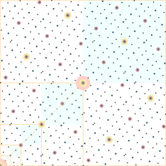
Refer to caption Refer to caption Refer to caption Refer to caption
Figure 6. Structure, generating matrices, points, and periodograms of various self-similar ξ𝜉\xi-sequences. The plots to the left depict the first few points; larger circles show the points closer to the beginning of the sequence. The top plots show the ξ0subscript𝜉0\xi_{0}-sequence generated by X=Y=(1,0,,0)𝑋𝑌100X=Y=(1,0,\dots,0).

We start with the geometric design requirements. After extensive experiments in trying to design a self-similar sequence, we settled for the following idea. We are looking for an infinite dyadic sequence such that every fourth point belongs to the bottom-left quadrant [0,1/2)2superscript0122[0,1/2)^{2} and for each k=0,1,2,𝑘012k=0,1,2,\dots the first 2ksuperscript2𝑘2^{k} points appearing in this quadrant form a scaled version of the first 2ksuperscript2𝑘2^{k} points of the whole sequence in [0,1)2superscript012[0,1)^{2}, with the same order. See Fig. 6 to the top-left. One can formulate this design requirement as

(15) p4i=pi/2for i=0,1,2,.formulae-sequencesubscript𝑝4𝑖subscript𝑝𝑖2for 𝑖012p_{4i}=p_{i}/2\qquad\text{for }i=0,1,2,\dots\,.

This means that a point with four times the sequence number is scaled by the factor 1/2121/2. In practice, we restrict ourselves to finite digital dyadic sequences. A digital dyadic sequence p0,p1,,p2m1subscript𝑝0subscript𝑝1subscript𝑝superscript2𝑚1p_{0},p_{1},\dots,p_{2^{m}-1} is called self-similar if for each i<2m2𝑖superscript2𝑚2i<2^{m-2} we have (15) with the right side truncated to m𝑚m digits (i.e., if the (m+1)𝑚1(m+1)-th digit after the point in the dyadic decomposition of one of the coordinates of pi/2subscript𝑝𝑖2p_{i}/2 is 111 then it is replaced by 00). This simple equation is all that we need to realize the sequence digitally.

We break it down into three elements. First, we note that multiplying the sequence number by 444 means shifting the bit vector S𝑆S down two steps, inserting two leading zeros that effectively wipe out two columns of the progressive matrix Cxsubscript𝐶𝑥C_{x}. Second, (15) means that the subsequent columns of the matrix should bear similar information to the wiped ones. Finally, dividing the coordinates by 2 is equivalent to pushing all these subsequent columns one row down, inserting zeros. This leads to the following self-similar matrix structure

(16) Cx=(a0b0000a1b1a0b00a2b2a1b1a0a3b3a2b2a1a4b4a3b3a2),subscript𝐶𝑥subscript𝑎0subscript𝑏0000missing-subexpressionmissing-subexpressionmissing-subexpressionmissing-subexpressionmissing-subexpressionmissing-subexpressionsubscript𝑎1subscript𝑏1subscript𝑎0subscript𝑏00missing-subexpressionmissing-subexpressionmissing-subexpressionmissing-subexpressionmissing-subexpressionmissing-subexpressionsubscript𝑎2subscript𝑏2subscript𝑎1subscript𝑏1subscript𝑎0missing-subexpressionmissing-subexpressionmissing-subexpressionmissing-subexpressionmissing-subexpressionmissing-subexpressionsubscript𝑎3subscript𝑏3subscript𝑎2subscript𝑏2subscript𝑎1missing-subexpressionmissing-subexpressionmissing-subexpressionmissing-subexpressionmissing-subexpressionmissing-subexpressionsubscript𝑎4subscript𝑏4subscript𝑎3subscript𝑏3subscript𝑎2C_{x}=\left(\begin{array}[]{cccccc}a_{0}&\vrule\lx@intercol\hfil{\color[rgb]{1,0,0}\definecolor[named]{pgfstrokecolor}{rgb}{1,0,0}b_{0}}\hfil\lx@intercol&\vrule\lx@intercol\hfil\color[rgb]{.75,.75,.75}\definecolor[named]{pgfstrokecolor}{rgb}{.75,.75,.75}\pgfsys@color@gray@stroke{.75}\pgfsys@color@gray@fill{.75}0\hfil\lx@intercol&\vrule\lx@intercol\hfil\color[rgb]{.75,.75,.75}\definecolor[named]{pgfstrokecolor}{rgb}{.75,.75,.75}\pgfsys@color@gray@stroke{.75}\pgfsys@color@gray@fill{.75}0\hfil\lx@intercol&\vrule\lx@intercol\hfil\color[rgb]{.75,.75,.75}\definecolor[named]{pgfstrokecolor}{rgb}{.75,.75,.75}\pgfsys@color@gray@stroke{.75}\pgfsys@color@gray@fill{.75}0\hfil\lx@intercol&\cdots\\ \cline{1-1}\cr a_{1}&{\color[rgb]{1,0,0}\definecolor[named]{pgfstrokecolor}{rgb}{1,0,0}b_{1}}&\vrule\lx@intercol\hfil a_{0}\hfil\lx@intercol&\vrule\lx@intercol\hfil b_{0}\hfil\lx@intercol&\vrule\lx@intercol\hfil\color[rgb]{.75,.75,.75}\definecolor[named]{pgfstrokecolor}{rgb}{.75,.75,.75}\pgfsys@color@gray@stroke{.75}\pgfsys@color@gray@fill{.75}0\hfil\lx@intercol&\cdots\\ \cline{1-2}\cr a_{2}&{\color[rgb]{1,0,0}\definecolor[named]{pgfstrokecolor}{rgb}{1,0,0}b_{2}}&a_{1}&\vrule\lx@intercol\hfil b_{1}\hfil\lx@intercol&\vrule\lx@intercol\hfil a_{0}\hfil\lx@intercol&\cdots\\ \cline{1-3}\cr a_{3}&{\color[rgb]{1,0,0}\definecolor[named]{pgfstrokecolor}{rgb}{1,0,0}b_{3}}&a_{2}&b_{2}&\vrule\lx@intercol\hfil a_{1}\hfil\lx@intercol&\cdots\\ \cline{1-4}\cr a_{4}&{\color[rgb]{1,0,0}\definecolor[named]{pgfstrokecolor}{rgb}{1,0,0}b_{4}}&a_{3}&b_{3}&a_{2}&\cdots\\ \vdots&\vdots&\vdots&\vdots&\vdots&\ddots\end{array}\right)\,,

for some column bit vectors A=(a0,a1,)𝐴subscript𝑎0subscript𝑎1A=(a_{0},a_{1},\cdots) and B=(b0,b1,)𝐵subscript𝑏0subscript𝑏1B=(b_{0},b_{1},\cdots) that, by definition, represent the x𝑥x-coordinates of the second and third point in the sequence (equal to 0.a0a1formulae-sequence0subscript𝑎0subscript𝑎10.a_{0}a_{1}\dots and 0.b0b1formulae-sequence0subscript𝑏0subscript𝑏10.b_{0}b_{1}\dots respectively). We take A𝐴A as a design parameter that can be freely chosen by the user, except for a0subscript𝑎0a_{0} which has to be 111. It then remains to set or compute the bits of B𝐵B so as to ensure a progressive matrix. We can iteratively expand the matrix. The key insight is that each subsequent expansion includes only one new unknown bit from B𝐵B, except for the first step where we have two bits when expanding from a 1×1111\times 1 to a 2×2222\times 2 matrix. Formally, we have the following statement:

Lemma 5.1.

For each bit vector A=(1,a1,a2,,am1)𝐴1subscript𝑎1subscript𝑎2subscript𝑎𝑚1A=(1,a_{1},a_{2},\cdots,a_{m-1}) starting with bit 111 there are exactly two bit vectors B=(b0,b1,,bm1)𝐵subscript𝑏0subscript𝑏1subscript𝑏𝑚1B=(b_{0},b_{1},\cdots,b_{m-1}) such that matrix (16) is progressive.

Proof.

Take an arbitrary bit b0subscript𝑏0b_{0} and let us determine bits b1,b2,subscript𝑏1subscript𝑏2b_{1},b_{2},\dots inductively.

Assume that b0,,bk1subscript𝑏0subscript𝑏𝑘1b_{0},\dots,b_{k-1} have already been determined so that the first k𝑘k leading principal minors of the matrix in Eq. (16) equal 111. Let us show that then there is a unique bksubscript𝑏𝑘b_{k} such that the (k+1)𝑘1(k+1)-th leading principal minor ΔΔ\Delta equals 111; for clarity, we illustrate the argument for k=3𝑘3k=3. Take the Laplace expansion along the last row:

Δ=|1b000a1b11b0a2b2a1b1a3b3a2b2|=a3|b000b11b0b2a1b1|++b3|100a11b0a2a1b1|+a2|1b00a1b1b0a2b2b1|+b2|1b00a1b11a2b2a1|.Δ1subscript𝑏000subscript𝑎1subscript𝑏11subscript𝑏0subscript𝑎2subscript𝑏2subscript𝑎1subscript𝑏1subscript𝑎3subscript𝑏3subscript𝑎2subscript𝑏2subscript𝑎3subscript𝑏000subscript𝑏11subscript𝑏0subscript𝑏2subscript𝑎1subscript𝑏1subscript𝑏3100subscript𝑎11subscript𝑏0subscript𝑎2subscript𝑎1subscript𝑏1subscript𝑎21subscript𝑏00subscript𝑎1subscript𝑏1subscript𝑏0subscript𝑎2subscript𝑏2subscript𝑏1subscript𝑏21subscript𝑏00subscript𝑎1subscript𝑏11subscript𝑎2subscript𝑏2subscript𝑎1\Delta=\left|\begin{array}[]{cccc}1&b_{0}&\color[rgb]{.75,.75,.75}\definecolor[named]{pgfstrokecolor}{rgb}{.75,.75,.75}\pgfsys@color@gray@stroke{.75}\pgfsys@color@gray@fill{.75}0&\color[rgb]{.75,.75,.75}\definecolor[named]{pgfstrokecolor}{rgb}{.75,.75,.75}\pgfsys@color@gray@stroke{.75}\pgfsys@color@gray@fill{.75}0\\ a_{1}&b_{1}&1&b_{0}\\ a_{2}&b_{2}&a_{1}&b_{1}\\ a_{3}&b_{3}&a_{2}&b_{2}\end{array}\right|=a_{3}\left|\begin{array}[]{ccc}b_{0}&\color[rgb]{.75,.75,.75}\definecolor[named]{pgfstrokecolor}{rgb}{.75,.75,.75}\pgfsys@color@gray@stroke{.75}\pgfsys@color@gray@fill{.75}0&\color[rgb]{.75,.75,.75}\definecolor[named]{pgfstrokecolor}{rgb}{.75,.75,.75}\pgfsys@color@gray@stroke{.75}\pgfsys@color@gray@fill{.75}0\\ b_{1}&1&b_{0}\\ b_{2}&a_{1}&b_{1}\end{array}\right|+\\ +b_{3}\left|\begin{array}[]{ccc}1&\color[rgb]{.75,.75,.75}\definecolor[named]{pgfstrokecolor}{rgb}{.75,.75,.75}\pgfsys@color@gray@stroke{.75}\pgfsys@color@gray@fill{.75}0&\color[rgb]{.75,.75,.75}\definecolor[named]{pgfstrokecolor}{rgb}{.75,.75,.75}\pgfsys@color@gray@stroke{.75}\pgfsys@color@gray@fill{.75}0\\ a_{1}&1&b_{0}\\ a_{2}&a_{1}&b_{1}\end{array}\right|+a_{2}\left|\begin{array}[]{ccc}1&b_{0}&\color[rgb]{.75,.75,.75}\definecolor[named]{pgfstrokecolor}{rgb}{.75,.75,.75}\pgfsys@color@gray@stroke{.75}\pgfsys@color@gray@fill{.75}0\\ a_{1}&b_{1}&b_{0}\\ a_{2}&b_{2}&b_{1}\end{array}\right|+b_{2}\left|\begin{array}[]{ccc}1&b_{0}&\color[rgb]{.75,.75,.75}\definecolor[named]{pgfstrokecolor}{rgb}{.75,.75,.75}\pgfsys@color@gray@stroke{.75}\pgfsys@color@gray@fill{.75}0\\ a_{1}&b_{1}&1\\ a_{2}&b_{2}&a_{1}\end{array}\right|.

By the structure of the matrix in Eq. (16), the coefficient at bksubscript𝑏𝑘b_{k} here

|100a11b0a2a1b1|=|1b0a1b1|100subscript𝑎11subscript𝑏0subscript𝑎2subscript𝑎1subscript𝑏11subscript𝑏0subscript𝑎1subscript𝑏1\left|\begin{array}[]{ccc}1&\color[rgb]{.75,.75,.75}\definecolor[named]{pgfstrokecolor}{rgb}{.75,.75,.75}\pgfsys@color@gray@stroke{.75}\pgfsys@color@gray@fill{.75}0&\color[rgb]{.75,.75,.75}\definecolor[named]{pgfstrokecolor}{rgb}{.75,.75,.75}\pgfsys@color@gray@stroke{.75}\pgfsys@color@gray@fill{.75}0\\ a_{1}&1&b_{0}\\ a_{2}&a_{1}&b_{1}\end{array}\right|=\left|\begin{array}[]{cc}1&b_{0}\\ a_{1}&b_{1}\end{array}\right|

is exactly the (k1)×(k1)𝑘1𝑘1(k-1)\times(k-1) leading principal minor, equal to 111 by the inductive hypothesis. Thus there is a unique bksubscript𝑏𝑘b_{k} such that Δ=1Δ1\Delta=1. Note that we compute the determinant of a (k+1)×(k+1)𝑘1𝑘1(k+1)\times(k+1) matrix using the assumption for the (k1)×(k1)𝑘1𝑘1(k-1)\times(k-1) matrix. Depending on k𝑘k being even or odd the matrix structure is slightly different, and we only illustrate the case for k𝑘k being odd here, but the even case is analogous. ∎

Similarly to the case of arbitrary progressive matrices in Section 3, there is a closed-form solution for the self-similar case. Starting with the simpler case A=(1,0,0,)𝐴100A=(1,0,0,\dots), i.e. setting the x𝑥x-coordinate of the second point in the sequence to be 1/2=0.100120.1001/2=0.100\dots, we get the following assertion: if A=(1,0,0,)𝐴100A=(1,0,0,\dots) in progressive matrix (16), then B𝐵B is one of the vectors

(17) (0,ξ1,ξ2,)0subscript𝜉1subscript𝜉2\displaystyle(0,\xi_{1},\xi_{2},\dots) =(0,1,1,0,1,0,0,0,1,0,0,0,0,0,0,0,1,),absent01101000100000001\displaystyle=(0,1,1,0,1,0,0,0,1,0,0,0,0,0,0,0,1,\dots)\,,
(18) (1,ξ1,ξ2,)1subscript𝜉1subscript𝜉2\displaystyle(1,\xi_{1},\xi_{2},\dots) =(1,1,1,0,1,0,0,0,1,0,0,0,0,0,0,0,1,),absent11101000100000001\displaystyle=(1,1,1,0,1,0,0,0,1,0,0,0,0,0,0,0,1,\dots),

where ξi=1subscript𝜉𝑖1\xi_{i}=1 if and only if i𝑖i is a power of 222. In other words, the third point of the sequence has one of the (truncated) x𝑥x-coordinates

(19) ξ𝜉\displaystyle\xi =0.01101000100000001=12k=022k,absent0.0110100010000000112superscriptsubscript𝑘0superscript2superscript2𝑘\displaystyle=0.01101000100000001\ldots=\frac{1}{2}\sum_{k=0}^{\infty}2^{-2^{k}}\,,
(20) ξ+superscript𝜉\displaystyle\xi^{+} =0.11101000100000001=12+12k=022k.absent0.111010001000000011212superscriptsubscript𝑘0superscript2superscript2𝑘\displaystyle=0.11101000100000001\ldots=\frac{1}{2}+\frac{1}{2}\sum_{k=0}^{\infty}2^{-2^{k}}\,.

This is proved by induction similarly to Lemma 5.1. This gives us the following self-similar progressive matrix:

(21) Cξ=(1000000000011000000001011000000001011000010001011000010001010000010001000000010001000000010001000000),subscript𝐶𝜉1000000000011000000001011000000001011000010001011000010001010000010001000000010001000000010001000000C_{\xi}=\left(\begin{array}[]{ccccccccccc}1&\color[rgb]{.75,.75,.75}\definecolor[named]{pgfstrokecolor}{rgb}{.75,.75,.75}\pgfsys@color@gray@stroke{.75}\pgfsys@color@gray@fill{.75}0&\color[rgb]{.75,.75,.75}\definecolor[named]{pgfstrokecolor}{rgb}{.75,.75,.75}\pgfsys@color@gray@stroke{.75}\pgfsys@color@gray@fill{.75}0&\color[rgb]{.75,.75,.75}\definecolor[named]{pgfstrokecolor}{rgb}{.75,.75,.75}\pgfsys@color@gray@stroke{.75}\pgfsys@color@gray@fill{.75}0&\color[rgb]{.75,.75,.75}\definecolor[named]{pgfstrokecolor}{rgb}{.75,.75,.75}\pgfsys@color@gray@stroke{.75}\pgfsys@color@gray@fill{.75}0&\color[rgb]{.75,.75,.75}\definecolor[named]{pgfstrokecolor}{rgb}{.75,.75,.75}\pgfsys@color@gray@stroke{.75}\pgfsys@color@gray@fill{.75}0&\color[rgb]{.75,.75,.75}\definecolor[named]{pgfstrokecolor}{rgb}{.75,.75,.75}\pgfsys@color@gray@stroke{.75}\pgfsys@color@gray@fill{.75}0&\color[rgb]{.75,.75,.75}\definecolor[named]{pgfstrokecolor}{rgb}{.75,.75,.75}\pgfsys@color@gray@stroke{.75}\pgfsys@color@gray@fill{.75}0&\color[rgb]{.75,.75,.75}\definecolor[named]{pgfstrokecolor}{rgb}{.75,.75,.75}\pgfsys@color@gray@stroke{.75}\pgfsys@color@gray@fill{.75}0&\color[rgb]{.75,.75,.75}\definecolor[named]{pgfstrokecolor}{rgb}{.75,.75,.75}\pgfsys@color@gray@stroke{.75}\pgfsys@color@gray@fill{.75}0&\cdots\\ \color[rgb]{.75,.75,.75}\definecolor[named]{pgfstrokecolor}{rgb}{.75,.75,.75}\pgfsys@color@gray@stroke{.75}\pgfsys@color@gray@fill{.75}0&1&1&\color[rgb]{.75,.75,.75}\definecolor[named]{pgfstrokecolor}{rgb}{.75,.75,.75}\pgfsys@color@gray@stroke{.75}\pgfsys@color@gray@fill{.75}0&\color[rgb]{.75,.75,.75}\definecolor[named]{pgfstrokecolor}{rgb}{.75,.75,.75}\pgfsys@color@gray@stroke{.75}\pgfsys@color@gray@fill{.75}0&\color[rgb]{.75,.75,.75}\definecolor[named]{pgfstrokecolor}{rgb}{.75,.75,.75}\pgfsys@color@gray@stroke{.75}\pgfsys@color@gray@fill{.75}0&\color[rgb]{.75,.75,.75}\definecolor[named]{pgfstrokecolor}{rgb}{.75,.75,.75}\pgfsys@color@gray@stroke{.75}\pgfsys@color@gray@fill{.75}0&\color[rgb]{.75,.75,.75}\definecolor[named]{pgfstrokecolor}{rgb}{.75,.75,.75}\pgfsys@color@gray@stroke{.75}\pgfsys@color@gray@fill{.75}0&\color[rgb]{.75,.75,.75}\definecolor[named]{pgfstrokecolor}{rgb}{.75,.75,.75}\pgfsys@color@gray@stroke{.75}\pgfsys@color@gray@fill{.75}0&\color[rgb]{.75,.75,.75}\definecolor[named]{pgfstrokecolor}{rgb}{.75,.75,.75}\pgfsys@color@gray@stroke{.75}\pgfsys@color@gray@fill{.75}0&\cdots\\ \color[rgb]{.75,.75,.75}\definecolor[named]{pgfstrokecolor}{rgb}{.75,.75,.75}\pgfsys@color@gray@stroke{.75}\pgfsys@color@gray@fill{.75}0&1&\color[rgb]{.75,.75,.75}\definecolor[named]{pgfstrokecolor}{rgb}{.75,.75,.75}\pgfsys@color@gray@stroke{.75}\pgfsys@color@gray@fill{.75}0&1&1&\color[rgb]{.75,.75,.75}\definecolor[named]{pgfstrokecolor}{rgb}{.75,.75,.75}\pgfsys@color@gray@stroke{.75}\pgfsys@color@gray@fill{.75}0&\color[rgb]{.75,.75,.75}\definecolor[named]{pgfstrokecolor}{rgb}{.75,.75,.75}\pgfsys@color@gray@stroke{.75}\pgfsys@color@gray@fill{.75}0&\color[rgb]{.75,.75,.75}\definecolor[named]{pgfstrokecolor}{rgb}{.75,.75,.75}\pgfsys@color@gray@stroke{.75}\pgfsys@color@gray@fill{.75}0&\color[rgb]{.75,.75,.75}\definecolor[named]{pgfstrokecolor}{rgb}{.75,.75,.75}\pgfsys@color@gray@stroke{.75}\pgfsys@color@gray@fill{.75}0&\color[rgb]{.75,.75,.75}\definecolor[named]{pgfstrokecolor}{rgb}{.75,.75,.75}\pgfsys@color@gray@stroke{.75}\pgfsys@color@gray@fill{.75}0&\cdots\\ \color[rgb]{.75,.75,.75}\definecolor[named]{pgfstrokecolor}{rgb}{.75,.75,.75}\pgfsys@color@gray@stroke{.75}\pgfsys@color@gray@fill{.75}0&\color[rgb]{.75,.75,.75}\definecolor[named]{pgfstrokecolor}{rgb}{.75,.75,.75}\pgfsys@color@gray@stroke{.75}\pgfsys@color@gray@fill{.75}0&\color[rgb]{.75,.75,.75}\definecolor[named]{pgfstrokecolor}{rgb}{.75,.75,.75}\pgfsys@color@gray@stroke{.75}\pgfsys@color@gray@fill{.75}0&1&\color[rgb]{.75,.75,.75}\definecolor[named]{pgfstrokecolor}{rgb}{.75,.75,.75}\pgfsys@color@gray@stroke{.75}\pgfsys@color@gray@fill{.75}0&1&1&\color[rgb]{.75,.75,.75}\definecolor[named]{pgfstrokecolor}{rgb}{.75,.75,.75}\pgfsys@color@gray@stroke{.75}\pgfsys@color@gray@fill{.75}0&\color[rgb]{.75,.75,.75}\definecolor[named]{pgfstrokecolor}{rgb}{.75,.75,.75}\pgfsys@color@gray@stroke{.75}\pgfsys@color@gray@fill{.75}0&\color[rgb]{.75,.75,.75}\definecolor[named]{pgfstrokecolor}{rgb}{.75,.75,.75}\pgfsys@color@gray@stroke{.75}\pgfsys@color@gray@fill{.75}0&\cdots\\ \color[rgb]{.75,.75,.75}\definecolor[named]{pgfstrokecolor}{rgb}{.75,.75,.75}\pgfsys@color@gray@stroke{.75}\pgfsys@color@gray@fill{.75}0&1&\color[rgb]{.75,.75,.75}\definecolor[named]{pgfstrokecolor}{rgb}{.75,.75,.75}\pgfsys@color@gray@stroke{.75}\pgfsys@color@gray@fill{.75}0&\color[rgb]{.75,.75,.75}\definecolor[named]{pgfstrokecolor}{rgb}{.75,.75,.75}\pgfsys@color@gray@stroke{.75}\pgfsys@color@gray@fill{.75}0&\color[rgb]{.75,.75,.75}\definecolor[named]{pgfstrokecolor}{rgb}{.75,.75,.75}\pgfsys@color@gray@stroke{.75}\pgfsys@color@gray@fill{.75}0&1&\color[rgb]{.75,.75,.75}\definecolor[named]{pgfstrokecolor}{rgb}{.75,.75,.75}\pgfsys@color@gray@stroke{.75}\pgfsys@color@gray@fill{.75}0&1&1&\color[rgb]{.75,.75,.75}\definecolor[named]{pgfstrokecolor}{rgb}{.75,.75,.75}\pgfsys@color@gray@stroke{.75}\pgfsys@color@gray@fill{.75}0&\cdots\\ \color[rgb]{.75,.75,.75}\definecolor[named]{pgfstrokecolor}{rgb}{.75,.75,.75}\pgfsys@color@gray@stroke{.75}\pgfsys@color@gray@fill{.75}0&\color[rgb]{.75,.75,.75}\definecolor[named]{pgfstrokecolor}{rgb}{.75,.75,.75}\pgfsys@color@gray@stroke{.75}\pgfsys@color@gray@fill{.75}0&\color[rgb]{.75,.75,.75}\definecolor[named]{pgfstrokecolor}{rgb}{.75,.75,.75}\pgfsys@color@gray@stroke{.75}\pgfsys@color@gray@fill{.75}0&1&\color[rgb]{.75,.75,.75}\definecolor[named]{pgfstrokecolor}{rgb}{.75,.75,.75}\pgfsys@color@gray@stroke{.75}\pgfsys@color@gray@fill{.75}0&\color[rgb]{.75,.75,.75}\definecolor[named]{pgfstrokecolor}{rgb}{.75,.75,.75}\pgfsys@color@gray@stroke{.75}\pgfsys@color@gray@fill{.75}0&\color[rgb]{.75,.75,.75}\definecolor[named]{pgfstrokecolor}{rgb}{.75,.75,.75}\pgfsys@color@gray@stroke{.75}\pgfsys@color@gray@fill{.75}0&1&\color[rgb]{.75,.75,.75}\definecolor[named]{pgfstrokecolor}{rgb}{.75,.75,.75}\pgfsys@color@gray@stroke{.75}\pgfsys@color@gray@fill{.75}0&1&\cdots\\ \color[rgb]{.75,.75,.75}\definecolor[named]{pgfstrokecolor}{rgb}{.75,.75,.75}\pgfsys@color@gray@stroke{.75}\pgfsys@color@gray@fill{.75}0&\color[rgb]{.75,.75,.75}\definecolor[named]{pgfstrokecolor}{rgb}{.75,.75,.75}\pgfsys@color@gray@stroke{.75}\pgfsys@color@gray@fill{.75}0&\color[rgb]{.75,.75,.75}\definecolor[named]{pgfstrokecolor}{rgb}{.75,.75,.75}\pgfsys@color@gray@stroke{.75}\pgfsys@color@gray@fill{.75}0&\color[rgb]{.75,.75,.75}\definecolor[named]{pgfstrokecolor}{rgb}{.75,.75,.75}\pgfsys@color@gray@stroke{.75}\pgfsys@color@gray@fill{.75}0&\color[rgb]{.75,.75,.75}\definecolor[named]{pgfstrokecolor}{rgb}{.75,.75,.75}\pgfsys@color@gray@stroke{.75}\pgfsys@color@gray@fill{.75}0&1&\color[rgb]{.75,.75,.75}\definecolor[named]{pgfstrokecolor}{rgb}{.75,.75,.75}\pgfsys@color@gray@stroke{.75}\pgfsys@color@gray@fill{.75}0&\color[rgb]{.75,.75,.75}\definecolor[named]{pgfstrokecolor}{rgb}{.75,.75,.75}\pgfsys@color@gray@stroke{.75}\pgfsys@color@gray@fill{.75}0&\color[rgb]{.75,.75,.75}\definecolor[named]{pgfstrokecolor}{rgb}{.75,.75,.75}\pgfsys@color@gray@stroke{.75}\pgfsys@color@gray@fill{.75}0&1&\cdots\\ \color[rgb]{.75,.75,.75}\definecolor[named]{pgfstrokecolor}{rgb}{.75,.75,.75}\pgfsys@color@gray@stroke{.75}\pgfsys@color@gray@fill{.75}0&\color[rgb]{.75,.75,.75}\definecolor[named]{pgfstrokecolor}{rgb}{.75,.75,.75}\pgfsys@color@gray@stroke{.75}\pgfsys@color@gray@fill{.75}0&\color[rgb]{.75,.75,.75}\definecolor[named]{pgfstrokecolor}{rgb}{.75,.75,.75}\pgfsys@color@gray@stroke{.75}\pgfsys@color@gray@fill{.75}0&\color[rgb]{.75,.75,.75}\definecolor[named]{pgfstrokecolor}{rgb}{.75,.75,.75}\pgfsys@color@gray@stroke{.75}\pgfsys@color@gray@fill{.75}0&\color[rgb]{.75,.75,.75}\definecolor[named]{pgfstrokecolor}{rgb}{.75,.75,.75}\pgfsys@color@gray@stroke{.75}\pgfsys@color@gray@fill{.75}0&\color[rgb]{.75,.75,.75}\definecolor[named]{pgfstrokecolor}{rgb}{.75,.75,.75}\pgfsys@color@gray@stroke{.75}\pgfsys@color@gray@fill{.75}0&\color[rgb]{.75,.75,.75}\definecolor[named]{pgfstrokecolor}{rgb}{.75,.75,.75}\pgfsys@color@gray@stroke{.75}\pgfsys@color@gray@fill{.75}0&1&\color[rgb]{.75,.75,.75}\definecolor[named]{pgfstrokecolor}{rgb}{.75,.75,.75}\pgfsys@color@gray@stroke{.75}\pgfsys@color@gray@fill{.75}0&\color[rgb]{.75,.75,.75}\definecolor[named]{pgfstrokecolor}{rgb}{.75,.75,.75}\pgfsys@color@gray@stroke{.75}\pgfsys@color@gray@fill{.75}0&\cdots\\ \color[rgb]{.75,.75,.75}\definecolor[named]{pgfstrokecolor}{rgb}{.75,.75,.75}\pgfsys@color@gray@stroke{.75}\pgfsys@color@gray@fill{.75}0&1&\color[rgb]{.75,.75,.75}\definecolor[named]{pgfstrokecolor}{rgb}{.75,.75,.75}\pgfsys@color@gray@stroke{.75}\pgfsys@color@gray@fill{.75}0&\color[rgb]{.75,.75,.75}\definecolor[named]{pgfstrokecolor}{rgb}{.75,.75,.75}\pgfsys@color@gray@stroke{.75}\pgfsys@color@gray@fill{.75}0&\color[rgb]{.75,.75,.75}\definecolor[named]{pgfstrokecolor}{rgb}{.75,.75,.75}\pgfsys@color@gray@stroke{.75}\pgfsys@color@gray@fill{.75}0&\color[rgb]{.75,.75,.75}\definecolor[named]{pgfstrokecolor}{rgb}{.75,.75,.75}\pgfsys@color@gray@stroke{.75}\pgfsys@color@gray@fill{.75}0&\color[rgb]{.75,.75,.75}\definecolor[named]{pgfstrokecolor}{rgb}{.75,.75,.75}\pgfsys@color@gray@stroke{.75}\pgfsys@color@gray@fill{.75}0&\color[rgb]{.75,.75,.75}\definecolor[named]{pgfstrokecolor}{rgb}{.75,.75,.75}\pgfsys@color@gray@stroke{.75}\pgfsys@color@gray@fill{.75}0&\color[rgb]{.75,.75,.75}\definecolor[named]{pgfstrokecolor}{rgb}{.75,.75,.75}\pgfsys@color@gray@stroke{.75}\pgfsys@color@gray@fill{.75}0&1&\cdots\\ \color[rgb]{.75,.75,.75}\definecolor[named]{pgfstrokecolor}{rgb}{.75,.75,.75}\pgfsys@color@gray@stroke{.75}\pgfsys@color@gray@fill{.75}0&\color[rgb]{.75,.75,.75}\definecolor[named]{pgfstrokecolor}{rgb}{.75,.75,.75}\pgfsys@color@gray@stroke{.75}\pgfsys@color@gray@fill{.75}0&\color[rgb]{.75,.75,.75}\definecolor[named]{pgfstrokecolor}{rgb}{.75,.75,.75}\pgfsys@color@gray@stroke{.75}\pgfsys@color@gray@fill{.75}0&1&\color[rgb]{.75,.75,.75}\definecolor[named]{pgfstrokecolor}{rgb}{.75,.75,.75}\pgfsys@color@gray@stroke{.75}\pgfsys@color@gray@fill{.75}0&\color[rgb]{.75,.75,.75}\definecolor[named]{pgfstrokecolor}{rgb}{.75,.75,.75}\pgfsys@color@gray@stroke{.75}\pgfsys@color@gray@fill{.75}0&\color[rgb]{.75,.75,.75}\definecolor[named]{pgfstrokecolor}{rgb}{.75,.75,.75}\pgfsys@color@gray@stroke{.75}\pgfsys@color@gray@fill{.75}0&\color[rgb]{.75,.75,.75}\definecolor[named]{pgfstrokecolor}{rgb}{.75,.75,.75}\pgfsys@color@gray@stroke{.75}\pgfsys@color@gray@fill{.75}0&\color[rgb]{.75,.75,.75}\definecolor[named]{pgfstrokecolor}{rgb}{.75,.75,.75}\pgfsys@color@gray@stroke{.75}\pgfsys@color@gray@fill{.75}0&\color[rgb]{.75,.75,.75}\definecolor[named]{pgfstrokecolor}{rgb}{.75,.75,.75}\pgfsys@color@gray@stroke{.75}\pgfsys@color@gray@fill{.75}0&\cdots\\ \vdots&\vdots&\vdots&\vdots&\vdots&\vdots&\vdots&\vdots&\vdots&\vdots&\ddots\end{array}\right)\,,

and a similarly looking matrix for Cξ+subscript𝐶superscript𝜉C_{\xi^{+}}. Note that this matrix looks quite different from the conventional upper-triangular form of Sobol matrices. Note also that ξ𝜉\xi appears also along the diagonal.

Now we move to the general case, where we have

Lemma 5.2.

For arbitrary A=(1,a1,a2,)𝐴1subscript𝑎1subscript𝑎2A=(1,a_{1},a_{2},\dots) the two vectors

(22) B𝐵\displaystyle B =ξ(A):=(0,ξ1,a1ξ1+ξ2,a2ξ1+a1ξ2+ξ3,)absent𝜉𝐴assign0subscript𝜉1subscript𝑎1subscript𝜉1subscript𝜉2subscript𝑎2subscript𝜉1subscript𝑎1subscript𝜉2subscript𝜉3\displaystyle=\xi(A):=(0,\,\xi_{1},\,a_{1}\xi_{1}+\xi_{2},\,a_{2}\xi_{1}+a_{1}\xi_{2}+\xi_{3},\,\dots)\,
(23) B+superscript𝐵\displaystyle B^{+} =ξ+(A):=ξ(A)+Aabsentsuperscript𝜉𝐴assign𝜉𝐴𝐴\displaystyle=\xi^{+}(A):=\xi(A)+A

are all the vectors making matrix (16) progressive.

In other words, the x𝑥x-coordinate of the third point in the sequence is obtained by the carryless multiplication of the x𝑥x-coordinate of the second point by one of numbers (19)–(20), followed by usual multiplication by 222.

Proof.

Multiply Cξsubscript𝐶𝜉C_{\xi} (or Cξ+subscript𝐶superscript𝜉C_{\xi^{+}}) by the lower unitriangular matrix

(24) L=(100a110a2a11a3a2a1)𝐿100subscript𝑎110subscript𝑎2subscript𝑎11subscript𝑎3subscript𝑎2subscript𝑎1L=\left(\begin{array}[]{cccc}1&\color[rgb]{.75,.75,.75}\definecolor[named]{pgfstrokecolor}{rgb}{.75,.75,.75}\pgfsys@color@gray@stroke{.75}\pgfsys@color@gray@fill{.75}0&\color[rgb]{.75,.75,.75}\definecolor[named]{pgfstrokecolor}{rgb}{.75,.75,.75}\pgfsys@color@gray@stroke{.75}\pgfsys@color@gray@fill{.75}0&\cdots\\ a_{1}&1&\color[rgb]{.75,.75,.75}\definecolor[named]{pgfstrokecolor}{rgb}{.75,.75,.75}\pgfsys@color@gray@stroke{.75}\pgfsys@color@gray@fill{.75}0&\cdots\\ a_{2}&a_{1}&1&\cdots\\ a_{3}&a_{2}&a_{1}&\cdots\\ \vdots&\vdots&\vdots&\ddots\end{array}\right)

from the left. This keeps the matrix progressive (LU-decomposable), preserves structure (16), and places A𝐴A and ξ(A)𝜉𝐴\xi(A) (or ξ+(A)superscript𝜉𝐴\xi^{+}(A)) in the first two columns. Then the proof is concluded by Lemma 5.1. ∎

Denoting the corresponding matrix by Cξ(A):=LCξassignsubscript𝐶𝜉𝐴𝐿subscript𝐶𝜉C_{\xi(A)}:=LC_{\xi} and Cξ+(A):=LCξ+assignsubscript𝐶superscript𝜉𝐴𝐿subscript𝐶superscript𝜉C_{\xi^{+}(A)}:=LC_{\xi^{+}}, we have the following statement to put it together:

Theorem 5.3.

For any pair of bit vectors X𝑋X and Y𝑌Y starting from 111 in the first position, the pairs (Cξ(X),Cξ+(Y))subscript𝐶𝜉𝑋subscript𝐶superscript𝜉𝑌(C_{\xi(X)},C_{\xi^{+}(Y)}) and (Cξ+(X),Cξ(Y))subscript𝐶superscript𝜉𝑋subscript𝐶𝜉𝑌(C_{\xi^{+}(X)},C_{\xi(Y)}) are progressive. Conversely, each progressive pair of matrices of form (16) equals either (Cξ(X),Cξ+(Y))subscript𝐶𝜉𝑋subscript𝐶superscript𝜉𝑌(C_{\xi(X)},C_{\xi^{+}(Y)}) or (Cξ+(X),Cξ(Y))subscript𝐶superscript𝜉𝑋subscript𝐶𝜉𝑌(C_{\xi^{+}(X)},C_{\xi(Y)}) for some X𝑋X and Y𝑌Y starting from 111.

Refer to caption Refer to caption Refer to caption Refer to caption
(a) Minimum distance between points (b) Average distance to the closest neighbor (c) The same for the minimum distance >0.3absent0.3>0.3 (d) Star discrepancy
Figure 7. An exhaustive exploration of ξ𝜉\xi-sequences containing 256 points. Each pixel in the top-right square [1/2;1)2superscript1212[1/2;1)^{2} represents a possible position of the second point of the sequence, which uniquely determines the whole ξ𝜉\xi-sequence. There are 128×128128128128\times 128 pixels in total and 16K possible ξ𝜉\xi-sequences. The color depicts one of the (suitably normalized) quality measures (a)–(d) of the resulting ξ𝜉\xi-sequence. In (c), the average distance to the closest neighbor is shown only for the sequences such that the minimum distance is greater than 0.30.30.3; the remaining pixels are brown. A few best-quality representatives are in the insets; each red bold point depicts the second point in the sequence. For comparison, the same quality measures for the Sobol sequence are shown in the legends.
Proof.

By construction, the matrices Cξ(X),Cξ+(Y)subscript𝐶𝜉𝑋subscript𝐶superscript𝜉𝑌C_{\xi(X)},C_{\xi^{+}(Y)} have form (16) with (a0,b0)=(1,0)subscript𝑎0subscript𝑏010(a_{0},b_{0})=(1,0) and (1,1)11(1,1) respectively; i.e., our pair has form

((1000a1b110a2b2a1b1),(1100c1d111c2d2c1d1))1000subscript𝑎1subscript𝑏110subscript𝑎2subscript𝑏2subscript𝑎1subscript𝑏11100subscript𝑐1subscript𝑑111subscript𝑐2subscript𝑑2subscript𝑐1subscript𝑑1\left(\left(\begin{array}[]{ccccc}1&\color[rgb]{.75,.75,.75}\definecolor[named]{pgfstrokecolor}{rgb}{.75,.75,.75}\pgfsys@color@gray@stroke{.75}\pgfsys@color@gray@fill{.75}0&\color[rgb]{.75,.75,.75}\definecolor[named]{pgfstrokecolor}{rgb}{.75,.75,.75}\pgfsys@color@gray@stroke{.75}\pgfsys@color@gray@fill{.75}0&\color[rgb]{.75,.75,.75}\definecolor[named]{pgfstrokecolor}{rgb}{.75,.75,.75}\pgfsys@color@gray@stroke{.75}\pgfsys@color@gray@fill{.75}0&\cdots\\ a_{1}&b_{1}&1&\color[rgb]{.75,.75,.75}\definecolor[named]{pgfstrokecolor}{rgb}{.75,.75,.75}\pgfsys@color@gray@stroke{.75}\pgfsys@color@gray@fill{.75}0&\cdots\\ a_{2}&b_{2}&a_{1}&b_{1}&\cdots\\ \vdots&\vdots&\vdots&\vdots&\ddots\end{array}\right)\,,\left(\begin{array}[]{ccccc}1&1&\color[rgb]{.75,.75,.75}\definecolor[named]{pgfstrokecolor}{rgb}{.75,.75,.75}\pgfsys@color@gray@stroke{.75}\pgfsys@color@gray@fill{.75}0&\color[rgb]{.75,.75,.75}\definecolor[named]{pgfstrokecolor}{rgb}{.75,.75,.75}\pgfsys@color@gray@stroke{.75}\pgfsys@color@gray@fill{.75}0&\cdots\\ c_{1}&d_{1}&1&1&\cdots\\ c_{2}&d_{2}&c_{1}&d_{1}&\cdots\\ \vdots&\vdots&\vdots&\vdots&\ddots\end{array}\right)\right)

for some ai,bi,ci,disubscript𝑎𝑖subscript𝑏𝑖subscript𝑐𝑖subscript𝑑𝑖a_{i},b_{i},c_{i},d_{i}. The two matrices are themselves progressive by Lemma 5.2. It remains to prove that hybrid matrix (6) has determinant 111 for r=1,,k1𝑟1𝑘1r=1,\dots,k-1. We compute the determinant recursively. Since the first row of (6) is (1 0 0)10 0(1\,0\,\dots\,0) in our case, it follows that removing the first row and the first column preserves the determinant:

|1000a1b11.a2b2a1b11100c1d111c2d2c1d1|=|b110b2a1b1100d111d2c1d1|.1000missing-subexpressionmissing-subexpressionmissing-subexpressionmissing-subexpressionmissing-subexpressionsubscript𝑎1subscript𝑏11absentsubscript𝑎2subscript𝑏2subscript𝑎1subscript𝑏11100subscript𝑐1subscript𝑑111subscript𝑐2subscript𝑑2subscript𝑐1subscript𝑑1missing-subexpressionmissing-subexpressionmissing-subexpressionmissing-subexpressionsubscript𝑏110subscript𝑏2subscript𝑎1subscript𝑏1100subscript𝑑111subscript𝑑2subscript𝑐1subscript𝑑1\left|\begin{array}[]{ccccc}{1}&\color[rgb]{.75,.75,.75}\definecolor[named]{pgfstrokecolor}{rgb}{.75,.75,.75}\pgfsys@color@gray@stroke{.75}\pgfsys@color@gray@fill{.75}0&\color[rgb]{.75,.75,.75}\definecolor[named]{pgfstrokecolor}{rgb}{.75,.75,.75}\pgfsys@color@gray@stroke{.75}\pgfsys@color@gray@fill{.75}0&\color[rgb]{.75,.75,.75}\definecolor[named]{pgfstrokecolor}{rgb}{.75,.75,.75}\pgfsys@color@gray@stroke{.75}\pgfsys@color@gray@fill{.75}0&{\cdots}\\ \cline{2-5}\cr a_{1}&\vrule\lx@intercol\hfil b_{1}\hfil\lx@intercol&{1}&{.}&\lx@intercol\hfil\cdots\hfil\lx@intercol\vrule\lx@intercol\\ a_{2}&\vrule\lx@intercol\hfil b_{2}\hfil\lx@intercol&{a_{1}}&b_{1}&\lx@intercol\hfil\cdots\hfil\lx@intercol\vrule\lx@intercol\\ \vdots&\vrule\lx@intercol\hfil\vdots\hfil\lx@intercol&{\vdots}&\vdots&\lx@intercol\hfil\ddots\hfil\lx@intercol\vrule\lx@intercol\\ {1}&\vrule\lx@intercol\hfil 1\hfil\lx@intercol&\color[rgb]{.75,.75,.75}\definecolor[named]{pgfstrokecolor}{rgb}{.75,.75,.75}\pgfsys@color@gray@stroke{.75}\pgfsys@color@gray@fill{.75}0&\color[rgb]{.75,.75,.75}\definecolor[named]{pgfstrokecolor}{rgb}{.75,.75,.75}\pgfsys@color@gray@stroke{.75}\pgfsys@color@gray@fill{.75}0&\lx@intercol\hfil\cdots\hfil\lx@intercol\vrule\lx@intercol\\ c_{1}&\vrule\lx@intercol\hfil d_{1}\hfil\lx@intercol&{1}&1&\lx@intercol\hfil\cdots\hfil\lx@intercol\vrule\lx@intercol\\ c_{2}&\vrule\lx@intercol\hfil d_{2}\hfil\lx@intercol&{c_{1}}&d_{1}&\lx@intercol\hfil\cdots\hfil\lx@intercol\vrule\lx@intercol\\ \vdots&\vrule\lx@intercol\hfil\vdots\hfil\lx@intercol&{\vdots}&\vdots&\lx@intercol\hfil\ddots\hfil\lx@intercol\vrule\lx@intercol\\ \cline{2-5}\cr\end{array}\,\right|=\left|\,\begin{array}[]{cccc}\cline{1-4}\cr\vrule\lx@intercol\hfil b_{1}\hfil\lx@intercol&{1}&\color[rgb]{.75,.75,.75}\definecolor[named]{pgfstrokecolor}{rgb}{.75,.75,.75}\pgfsys@color@gray@stroke{.75}\pgfsys@color@gray@fill{.75}0&\lx@intercol\hfil\cdots\hfil\lx@intercol\vrule\lx@intercol\\ \vrule\lx@intercol\hfil b_{2}\hfil\lx@intercol&{a_{1}}&b_{1}&\lx@intercol\hfil\cdots\hfil\lx@intercol\vrule\lx@intercol\\ \vrule\lx@intercol\hfil\vdots\hfil\lx@intercol&{\vdots}&\vdots&\lx@intercol\hfil\ddots\hfil\lx@intercol\vrule\lx@intercol\\ \vrule\lx@intercol\hfil{\color[rgb]{1,0,0}\definecolor[named]{pgfstrokecolor}{rgb}{1,0,0}1}\hfil\lx@intercol&{\color[rgb]{1,0,0}\definecolor[named]{pgfstrokecolor}{rgb}{1,0,0}0}&{\color[rgb]{1,0,0}\definecolor[named]{pgfstrokecolor}{rgb}{1,0,0}0}&\lx@intercol\hfil{\color[rgb]{1,0,0}\definecolor[named]{pgfstrokecolor}{rgb}{1,0,0}\cdots}\hfil\lx@intercol\vrule\lx@intercol\\ \vrule\lx@intercol\hfil d_{1}\hfil\lx@intercol&{1}&1&\lx@intercol\hfil\cdots\hfil\lx@intercol\vrule\lx@intercol\\ \vrule\lx@intercol\hfil d_{2}\hfil\lx@intercol&{c_{1}}&d_{1}&\lx@intercol\hfil\cdots\hfil\lx@intercol\vrule\lx@intercol\\ \vrule\lx@intercol\hfil\vdots\hfil\lx@intercol&{\vdots}&\vdots&\lx@intercol\hfil\ddots\hfil\lx@intercol\vrule\lx@intercol\\ \cline{1-4}\cr\end{array}\,\right|.

In the resulting matrix, the (kr)𝑘𝑟(k-r)-th row (highlighted) becomes (1 0 0)10 0(1\,0\,\dots\,0). Now removing this row and the first column, we get

|b110b2a1b1100d111d2c1d1|=|10a1b111c1d1|.missing-subexpressionmissing-subexpressionmissing-subexpressionmissing-subexpressionsubscript𝑏110subscript𝑏2subscript𝑎1subscript𝑏1missing-subexpressionmissing-subexpressionmissing-subexpressionmissing-subexpression100missing-subexpressionmissing-subexpressionmissing-subexpressionmissing-subexpressionsubscript𝑑111subscript𝑑2subscript𝑐1subscript𝑑1missing-subexpressionmissing-subexpressionmissing-subexpression10subscript𝑎1subscript𝑏1missing-subexpressionmissing-subexpressionmissing-subexpressionmissing-subexpressionmissing-subexpressionmissing-subexpressionmissing-subexpressionmissing-subexpressionmissing-subexpression11subscript𝑐1subscript𝑑1\left|\begin{array}[]{cccc}\cline{2-4}\cr b_{1}&\vrule\lx@intercol\hfil 1\hfil\lx@intercol&\color[rgb]{.75,.75,.75}\definecolor[named]{pgfstrokecolor}{rgb}{.75,.75,.75}\pgfsys@color@gray@stroke{.75}\pgfsys@color@gray@fill{.75}0&\lx@intercol\hfil\cdots\hfil\lx@intercol\vrule\lx@intercol\\ b_{2}&\vrule\lx@intercol\hfil a_{1}\hfil\lx@intercol&b_{1}&\lx@intercol\hfil\cdots\hfil\lx@intercol\vrule\lx@intercol\\ \vdots&\vrule\lx@intercol\hfil\vdots\hfil\lx@intercol&\vdots&\lx@intercol\hfil\ddots\hfil\lx@intercol\vrule\lx@intercol\\ \cline{2-4}\cr{\color[rgb]{1,0,0}\definecolor[named]{pgfstrokecolor}{rgb}{1,0,0}1}&{\color[rgb]{1,0,0}\definecolor[named]{pgfstrokecolor}{rgb}{1,0,0}0}&{\color[rgb]{1,0,0}\definecolor[named]{pgfstrokecolor}{rgb}{1,0,0}0}&{\color[rgb]{1,0,0}\definecolor[named]{pgfstrokecolor}{rgb}{1,0,0}\cdots}\\ \cline{2-4}\cr d_{1}&\vrule\lx@intercol\hfil 1\hfil\lx@intercol&1&\lx@intercol\hfil\cdots\hfil\lx@intercol\vrule\lx@intercol\\ d_{2}&\vrule\lx@intercol\hfil c_{1}\hfil\lx@intercol&d_{1}&\lx@intercol\hfil\cdots\hfil\lx@intercol\vrule\lx@intercol\\ \vdots&\vrule\lx@intercol\hfil\vdots\hfil\lx@intercol&\vdots&\lx@intercol\hfil\ddots\hfil\lx@intercol\vrule\lx@intercol\\ \cline{2-4}\cr\end{array}\,\right|=\left|\,\begin{array}[]{ccc}\cline{1-3}\cr\vrule\lx@intercol\hfil{1}\hfil\lx@intercol&\color[rgb]{.75,.75,.75}\definecolor[named]{pgfstrokecolor}{rgb}{.75,.75,.75}\pgfsys@color@gray@stroke{.75}\pgfsys@color@gray@fill{.75}0&\lx@intercol\hfil{\cdots}\hfil\lx@intercol\vrule\lx@intercol\\ \vrule\lx@intercol\hfil a_{1}\hfil\lx@intercol&b_{1}&\lx@intercol\hfil\cdots\hfil\lx@intercol\vrule\lx@intercol\\ \vrule\lx@intercol\hfil\vdots\hfil\lx@intercol&\vdots&\lx@intercol\hfil\ddots\hfil\lx@intercol\vrule\lx@intercol\\ \cline{1-3}\cr\\[-8.5359pt] \cline{1-3}\cr\vrule\lx@intercol\hfil{1}\hfil\lx@intercol&{1}&\lx@intercol\hfil{\cdots}\hfil\lx@intercol\vrule\lx@intercol\\ \vrule\lx@intercol\hfil c_{1}\hfil\lx@intercol&d_{1}&\lx@intercol\hfil\cdots\hfil\lx@intercol\vrule\lx@intercol\\ \vrule\lx@intercol\hfil\vdots\hfil\lx@intercol&\vdots&\lx@intercol\hfil\ddots\hfil\lx@intercol\vrule\lx@intercol\\ \cline{1-3}\cr\end{array}\,\right|.

The resulting matrix has the same structure as initial matrix (6), only r𝑟r and k𝑘k are reduced by 111 and 222 respectively. We now repeat the procedure, each time removing the row (1 0 0)10 0(1\,0\,\dots\,0) and the first column in the current matrix until we get r=0𝑟0r=0 or r=k𝑟𝑘r=k. The resulting determinant will be a leading principal minor of Cξ(X)subscript𝐶𝜉𝑋C_{\xi(X)} or Cξ+(Y)subscript𝐶superscript𝜉𝑌C_{\xi^{+}(Y)}. It equals 111 because Cξ(X)subscript𝐶𝜉𝑋C_{\xi(X)} or Cξ+(Y)subscript𝐶superscript𝜉𝑌C_{\xi^{+}(Y)} are themselves progressive.

The converse assertion follows from Lemma 5.2 because the pairs (Cξ(X),Cξ(Y))subscript𝐶𝜉𝑋subscript𝐶𝜉𝑌(C_{\xi(X)},C_{\xi(Y)}) and (Cξ+(X),Cξ+(Y))subscript𝐶superscript𝜉𝑋subscript𝐶superscript𝜉𝑌(C_{\xi^{+}(X)},C_{\xi^{+}(Y)}) are never progressive. ∎

We find these results striking, since this constant ξ𝜉\xi handles all the effort of matrix derivation and pairing we encountered in Section 3. Thus, the resulting self-similar sequences generated by (Cξ(X),Cξ+(Y))subscript𝐶𝜉𝑋subscript𝐶superscript𝜉𝑌(C_{\xi(X)},C_{\xi^{+}(Y)}) for various X𝑋X and Y𝑌Y are deservedly called ξ𝜉\xi-sequences. See Fig. 6 and 7. (We do not need to consider the pairs (Cξ+(X),Cξ(Y))subscript𝐶superscript𝜉𝑋subscript𝐶𝜉𝑌(C_{\xi^{+}(X)},C_{\xi(Y)}) because this leads just to the swap of x𝑥x- and y𝑦y-coordinates.) The sequence generated by (Cξ,Cξ+)subscript𝐶𝜉subscript𝐶superscript𝜉(C_{\xi},C_{\xi^{+}}) is referred as ξ0subscript𝜉0\xi_{0}-sequence. On the practical side, we truncate the coordinates of the 2msuperscript2𝑚2^{m} points not to m𝑚m bits as required by the digital construction, but to the machine precision of M=32𝑀32M=32 (or M=64𝑀64M=64) bits. In other words, we always consider the first 2msuperscript2𝑚2^{m} points of a 2Msuperscript2𝑀2^{M}-point ξ𝜉\xi-sequence. We note that the special structure of ξ𝜉\xi reduces the carryless multiplication to O(logM)𝑂𝑀{O}\left(\log M\right) from O(M)𝑂𝑀{O}(M). In 32-bit precision, it takes precisely 555 shift-and-xor operations. This makes setting up a ξ𝜉\xi-sequence, given (X,Y)𝑋𝑌(X,Y), incredibly low-cost, even cheaper than generating a random sample for (X,Y)𝑋𝑌(X,Y). Algorithm 3 summarizes the preceding derivations into a set of steps for creating a ξ𝜉\xi-sequence.

Input :  Two bit-vectors X𝑋X and Y𝑌Y (the coordinates of p1subscript𝑝1p_{1});
Output : The first 444 points p0,,p3subscript𝑝0subscript𝑝3p_{0},\dots,p_{3} of the sequence.
1 ξ(A)(21+22+24+28+216)A𝜉𝐴superscript21superscript22superscript24superscript28superscript216𝐴\xi(A)\leftarrow(2^{-1}+2^{-2}+2^{-4}+2^{-8}+2^{-16})A;
2 Bξ(X)𝐵𝜉𝑋B\leftarrow\xi(X);
3 B+ξ(Y)+Ysuperscript𝐵𝜉𝑌𝑌B^{+}\leftarrow\xi(Y)+Y;
4 p0(0,0)subscript𝑝000p_{0}\leftarrow(0,0);
5 p1(X,Y)subscript𝑝1𝑋𝑌p_{1}\leftarrow(X,Y);
6 p2(B,B+)subscript𝑝2𝐵superscript𝐵p_{2}\leftarrow(B,B^{+});
p3(X,Y)+(B,B+)subscript𝑝3𝑋𝑌𝐵superscript𝐵p_{3}\leftarrow(X,Y)+(B,B^{+}).
Algorithm 3 Constructing the first 444 points of a ξ𝜉\xi-sequence using 32-bit precision from two bit-vectors X=(x0,)𝑋subscript𝑥0X=(x_{0},\dots) and Y=(y0,)𝑌subscript𝑦0Y=(y_{0},\dots) with x0=y0=1subscript𝑥0subscript𝑦01x_{0}=y_{0}=1. All additions and multiplications are carryless.
Point getSample(uint32_t seqNo) {
uint32_t x(0), y(0);
for (int depth = 0; depth < 16; depth++) {
x ^= p[seqNo & 3].x >> depth;
y ^= p[seqNo & 3].y >> depth;
seqNo >>= 2;
}
return {x, y};
}
Algorithm 4 C code for retrieving a sample from a ξ𝜉\xi-sequence. The sequence is encoded by the first 444 points p[0],,p[3]𝑝delimited-[]0𝑝delimited-[]3p[0],\dots,p[3]. The input is the number seqNo of the sample.

To our knowledge, ξ𝜉\xi-sequences are the fastest way to construct a dyadic sequence and draw different dyadic nets. They enable constructing a pseudo-random sequence for each pixel. However, the fast construction turns out to be not the only advantage: the self-similar structure actually embodies a wealth of versatility that we are going to discuss in the following subsections.

5.1. Retrieving the Samples

Points from ξ𝜉\xi-sequences may be generated from the matrices as any standard digital sequence. The self-similar structure of the matrices, however, offers a short-hand, as outlined in Algorithm 4.

Thus, besides fast construction, drawing the samples is an aspect where ξ𝜉\xi-sequences significantly stand out compared to all alternatives we are aware of. The simple loop structure of ξ𝜉\xi-sequences, and the few parameters, make it a good candidate for low-level optimization, using registers, for example, but our plain C code already delivers high performance, as depicted in Table 4.

Table 4. Speed performance, in million points per second, of ξ𝜉\xi-sequences and other state-of-the-art sampler generators.
m=log2(N)𝑚subscript2𝑁m=\log_{2}(N) 8 12 16 20 24 28
Random 18 25 24 56 68 71
Sobol 32 35 28 53 57 51
Burley 11 16 13 31 39 39
ξ𝜉\xi 17 26 24 57 74 73
ξ256subscript𝜉256\xi_{256} 32 113 146 185 411 410

While the straightforward implementation of ξ𝜉\xi-sequences shown in Algorithm 4 already leads the competition, the self-similar structure of the sequence permits ever further speed up through a small lookup table. In the basic implementation we derive the basis vectors from the first four points, but in fact any power-of-four number of points may be used in the same way as basis for retrieving subsequent points. The ξ256subscript𝜉256\xi_{256} entry in Table 4 refers to an implementation that uses a 256256256-vector look-up table, and it leads to 2-6×\times speed up.

5.2. Memory Footprint

In addition to their speed performance, ξ𝜉\xi-sequences consume very little memory, and offer a flexible trade-off between memory and speed. The sequence may be compressed to a single 2D bit vector p1subscript𝑝1{p}_{1}, a pair of vectors p1,p2subscript𝑝1subscript𝑝2p_{1},p_{2}, or the standard four vectors p0,,p3subscript𝑝0subscript𝑝3p_{0},\dots,p_{3}, and may be expanded to a 16, 256, or even 64K lookup table for two-step retrieval. This flexibility with memory makes ξ𝜉\xi-sequences quite GPU friendly. Indeed, providing random numbers in a GPU context is a standing challenge, and ξ𝜉\xi-sequences help in this direction by making it possible to run a unique random sequence in each thread, passing a table of parameters that identify the sequences. We implemented a test of this, and generated over 17G points per second, roughly 1T per minute, on a TITAN Xp GPU.
Refer to caption

(c) (0, 2)-Sequence

Refer to caption Refer to caption Refer to caption Refer to caption

(b) Random ξ𝜉\xi

Refer to caption Refer to caption Refer to caption Refer to caption

(a) Sobol

Refer to caption Refer to caption Refer to caption Refer to caption
2 SPP 8 SPP 16 SPP 32 SPP
Figure 8. Physically-based renderings using various digital dyadic sequences: (a) The Global Sobol sampler based on the Sobol sequence; (b) our adapted global sampler using a random ξ𝜉\xi-sequence; and (c) low-discrepancy (0,2)02(0,2)-sequence sampler, which uses independently shuffled Sobol 2D samples for each pixel and pair of dimensions. We placed our sampler in the middle for easier comparison. The figure shows that the ξ𝜉\xi-based Global sampler is less aliased than Sobol and less noisy than the pixel-based sampler. The insets show selected parts of the scene at different sampling rates.

Sobol

Refer to caption Refer to caption Refer to caption Refer to caption Refer to caption Refer to caption

ξ0subscript𝜉0\xi_{0}

Refer to caption Refer to caption Refer to caption Refer to caption Refer to caption Refer to caption
1 SPP 2 SPP 4 SPP 8 SPP 16 SPP 32 SPP
Figure 9. Renderings obtained with the Z-sampler from Ahmed and Wonka (2020) using Sobol and ξ0subscript𝜉0\xi_{0} sequences for the generation of the samples at difference sampling rates (samples per pixel). The figure shows that the ξ𝜉\xi-based Z-Sampler is less noisy than the Sobol-based one for the shown scene.

5.3. Morton Ordering

Instead of generating the x𝑥x and y𝑦y coordinates separately, they can be obtained jointly as a Morton-ordering (Morton, 1966) index

(25) 𝐳=0.y0x0y1x1,formulae-sequence𝐳0subscript𝑦0subscript𝑥0subscript𝑦1subscript𝑥1\mathbf{z}=0.y_{0}x_{0}y_{1}x_{1}\cdots\,,

and then we can split (unshuffle (Warren, 2012)) the bits later. This can be done easily by

(26) 𝐳(i+1)superscript𝐳𝑖1\displaystyle\mathbf{z}^{(i+1)} 𝐳(i)+pz[s(i)mod4]22i,absentsuperscript𝐳𝑖subscript𝑝𝑧delimited-[]modulosuperscript𝑠𝑖4superscript22𝑖\displaystyle\leftarrow\mathbf{z}^{(i)}+p_{z}[s^{(i)}\bmod 4]\cdot 2^{-2i}\,, 𝐬(i+1)superscript𝐬𝑖1\displaystyle\mathbf{s}^{(i+1)} 𝐬(i)/4absentsuperscript𝐬𝑖4\displaystyle\leftarrow\lfloor\mathbf{s}^{(i)}/4\rfloor\,

where i=0,,15𝑖015i=0,\dots,15, 𝐳(0)=0superscript𝐳00\mathbf{z}^{(0)}=0, 𝐬(0)superscript𝐬0\mathbf{s}^{(0)} is the point index in the sequence, pz[q]subscript𝑝𝑧delimited-[]𝑞p_{z}[q] is obtained by interleaving (shuffling (Warren, 2012)) the bits of y𝑦y- and x𝑥x-coordinates of the q𝑞q-th point p[q]𝑝delimited-[]𝑞p[q] for q=0,,3𝑞03q=0,\dots,3, and addition is carryless. This may not be very useful in generating the samples, because, in addition to the cost of unshuffle, it requires 64-bit processing to obtain the full 32-bit resolution of each axis. Mapping to Morton indices, however, is useful in the reverse direction, where we are given the coordinates of a stratum, and asked to retrieve the exact location of the (first) sample in that stratum, and/or its sequence number, as encountered in stippling and importance sampling. Note that the coordinates of the stratum prefix the coordinates of points inside it. Thus, obtaining a point sequence number, given the stratum, is a partial inversion of the sequence, which we discuss in more detail next.

5.4. Inverting the Sequence

A straightforward approach to inverting a ξ𝜉\xi-sequence, mapping a stratum index 𝐳𝐳\mathbf{z} into a sequence number 𝐬𝐬\mathbf{s}, is to undo the iterations in Eq. (26). Let

(27) 𝐬𝐬\displaystyle\mathbf{s} =s54s32s10,absentsubscript𝑠54subscript𝑠32subscript𝑠10\displaystyle=\cdots s_{54}s_{32}s_{10}\,,
(28) 𝐳𝐳\displaystyle\mathbf{z} =0.z01z23,formulae-sequenceabsent0subscript𝑧01subscript𝑧23\displaystyle=0.z_{01}z_{23}\cdots\,,
(29) pz[q]subscript𝑝𝑧delimited-[]𝑞\displaystyle p_{z}[q] =0.pz01[q]pz23[q]formulae-sequenceabsent0subscript𝑝𝑧01delimited-[]𝑞subscript𝑝𝑧23delimited-[]𝑞\displaystyle=0.p_{z01}[q]p_{z23}[q]\cdots\,

encode the sequence index of a point, its Morton index, and the first 444 points of the sequence written in base 444. Note the reversed indexing of the digits of the sequence number. Given 𝐳(0)=𝐳superscript𝐳0𝐳\mathbf{z}^{(0)}=\mathbf{z}, we may find 𝐬𝐬\mathbf{s} iteratively starting from 𝐬(0)=0superscript𝐬00\mathbf{s}^{(0)}=0 as follows:

(30) q𝑞\displaystyle q q:z01(i)=pz01[q],:absent𝑞superscriptsubscript𝑧01𝑖subscript𝑝𝑧01delimited-[]𝑞\displaystyle\leftarrow q:z_{01}^{(i)}=p_{z01}[q]\,,
(31) 𝐬(i+1)superscript𝐬𝑖1\displaystyle\mathbf{s}^{(i+1)} 𝐬(i)+q22i,absentsuperscript𝐬𝑖𝑞superscript22𝑖\displaystyle\leftarrow\mathbf{s}^{(i)}+q\cdot 2^{2i}\,,
(32) 𝐳(i+1)superscript𝐳𝑖1\displaystyle\mathbf{z}^{(i+1)} (𝐳(i)+pz[q])4,absentsuperscript𝐳𝑖subscript𝑝𝑧delimited-[]𝑞4\displaystyle\leftarrow(\mathbf{z}^{(i)}+p_{z}[q])\cdot 4\,,

in the i𝑖i-th iteration. The idea is that, if we examine Eq. (26), we see that only one vector contributes to the most significant two bits of 𝐳𝐳\mathbf{z}. We can therefore deduce which of the four vectors was added in the first iteration of computing 𝐳𝐳\mathbf{z}, and insert its index as a digit in the sequence number, as in Eq. (31). We then subtract, or equivalently add, the originally added vector to 𝐳𝐳\mathbf{z}. Now, only one vector is responsible for the following pair of bits. By shifting the bits up we can recursively apply the undo process. Note that this process iteratively zeros 𝐳𝐳\mathbf{z} while building 𝐬𝐬\mathbf{s}.

We implemented this and obtained the inversion rate of ~38M points per second (cf. Table 4) that, while faster than any sampling technique we are aware of, is significantly slower than the forward production rate. A much faster approach takes advantage of Morton ordering discussed in Section 5.3, noting that the inversion matrix bears a similar staggered pair-of-columns structure. This gives a speed up of up to 70% over the forward rate, since only one value is evaluated rather than two.

5.5. Coding Complexity

Again, this is an aspect where ξ𝜉\xi-sequences have an advantage. Not only the fact that their implementation follows straightforward steps, as listed in Algorithm 3, but the intuition of these steps has a clear geometric interpretation, as we discussed earlier.

5.6. Atlas

The relatively small two-dimensional space of ξ𝜉\xi-sequences, along with their easy implementation on GPUs, makes it possible to scan them exhaustively and build an atlas for exploring these patterns and finding ones with favorable properties. Fig. 7 shows example maps for the star discrepancy, minimum distance between points, and average distance to the nearest neighbor.

5.7. Rendering Examples

We show the impact of our work in two rendering examples.

The first example (Fig. 8) demonstrates that self-similar sequences provide better anti-aliasing than the standard Sobol sequence. To make a meaningful comparison we integrated the sequences into the Global Sobol Sampler coming with PBRT. The ξ𝜉\xi-sequences offer: (1) 3×\times speedup in sample generation and 5×\times in inversion, leading to up to 37% observed reduction in rendering times; (2) no inversion lookup tables, cf.(Grünschloß et al., 2012); (3) notable anti-aliasing with randomized ξ𝜉\xi-sequences, and (4) they are free; emphasizing the value of our in-depth study.

Let us make a few comments on the implementation. The sampler uses a higher-dimensional Sobol sequence, generated by certain matrices (I,P,C2,C3,)𝐼𝑃subscript𝐶2subscript𝐶3(I,P,C_{2},C_{3},\dots); the first two are used to sample the image plane. We transform the matrices so that the first two become generating matrices (Cξ(X),Cξ+(Y))subscript𝐶𝜉𝑋subscript𝐶superscript𝜉𝑌(C_{\xi(X)},C_{\xi^{+}(Y)}) of the desired ξ𝜉\xi-sequence. For that purpose, we decompose Cξ(X)=LxUsubscript𝐶𝜉𝑋subscript𝐿𝑥𝑈C_{\xi(X)}=L_{x}U and Cξ+(Y)=LyPUsubscript𝐶superscript𝜉𝑌subscript𝐿𝑦𝑃𝑈C_{\xi^{+}(Y)}=L_{y}PU as in Theorem 3.9. Then we right-multiply all the original matrices (I,P,C2,C3,)𝐼𝑃subscript𝐶2subscript𝐶3(I,P,C_{2},C_{3},\dots) by U𝑈U (which means just reordering of the sequence) and left-multiply the first two matrices by Lxsubscript𝐿𝑥L_{x} and Lysubscript𝐿𝑦L_{y} respectively (which means scrambling). The resulting sequence is used for sampling.

The second example (Fig. 9) also shows slightly better anti-aliasing. Here we integrated the sequences into the Z-Sampler (Ahmed and Wonka, 2020) that uses the samples as is, without any scrambling.
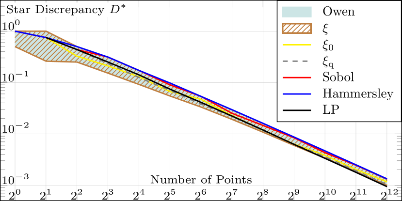
Refer to caption
Figure 10. Discrepancy comparison of XOR-scrambled ξ𝜉\xi-sequences to unscrambled Sobol sequence. Hammersley and Larcher-Pillichshammer (LP) nets are shown for comparison. For Owen and ξ𝜉\xi we measured the discrepancy over a randomly drawn 64K sample. The yellow line refers to the ξ0subscript𝜉0\xi_{0}-sequence. The dashed line ξqsubscript𝜉q\xi_{\text{q}} refers to the lowest measured discrepancy of the sampled sequences when the coordinates of the points are truncated to log2(Number of Points)subscript2Number of Points\log_{2}(\text{Number of Points}) bits.

5.8. Discrepancy and Spectral Evaluation

The new class of self-similar sequences introduced in the paper has several advantages, that we have evaluated in the preceding subsections, such as speed, memory usage, anti-aliasing, and versatility. Towards that, we show discrepancy and spectral comparison in Fig. 10 and 11, both demonstrating that ξ𝜉\xi-sequences are a good representative sample of the space of digital dyadic sequences. Note that all digital dyadic sequences exhibit some structure when looking at a single instance and the perceived structure changes with m𝑚m (see Fig. 1).

Refer to caption Refer to caption Refer to caption Refer to caption Refer to caption
(a) Owen (b) Burley (c) XOR-Scrambled Sobol (d) Random Digital (e) ξ𝜉\xi
Figure 11. Two-dimensional and radial average spectral profiles of different dyadic sequences, showing (top) the frequency power spectrum of the point process, obtained by averaging 16k periodograms of 256 points, and (bottom) a periodogram of a randomly selected realization. We use radial profiles advocated by (Ahmed et al., 2022), where we average values for every distinct radius. The set for ξ𝜉\xi-sequences includes all distinct sequences (up to XOR-scrambling) at 8-bit resolution. A randomly selected digital or ξ𝜉\xi-sequence has a smoother periodogram than the XOR-Scrambled Sobol sequence but not Burley’s implementation of Owen-scrambling. However, the average of sufficiently many periodograms for ξ𝜉\xi-sequence is smoother than both, and visually as smooth as Owen’s scrambling.

6. Discussion and Conclusion

In this paper, we presented new insights on digital dyadic sequences. Our work provides a comprehensive understanding of the design space and how to navigate it.

We believe our work will lay the foundation for future work in systematically exploring the design space of higher-dimensional sequences and their impact on rendering. The importance of 2D sequences is that they often serve as building blocks for synthesizing high-dimensional sequences. Throughout the paper, we already discussed multiple implications of our work on rendering applications, and we are hopeful that the proposed ξ𝜉\xi-sequences and Gray sequences will find their way into existing rendering frameworks.

Acknowledgements.
We are grateful to F. Pillichshammer for bringing earlier proofs of Theorems 3.6 and 3.9 (which we conceived independently) to our attention. Thanks to Mohanad Ahmed for his insightful discussions.

References

  • (1)
  • Ahmed et al. (2017) Abdalla G. M. Ahmed, Till Niese, Hui Huang, and Oliver Deussen. 2017. An Adaptive Point Sampler on a Regular Lattice. ACM Trans. Graph. 36, 4, Article 138 (July 2017), 13 pages. https://doi.org/10.1145/3072959.3073588
  • Ahmed et al. (2016) Abdalla G. M. Ahmed, Hélène Perrier, David Coeurjolly, Victor Ostromoukhov, Jianwei Guo, Dong-Ming Yan, Hui Huang, and Oliver Deussen. 2016. Low-Discrepancy Blue-Noise Sampling. ACM Trans. Graph. 35, 6, Article 247 (Nov. 2016), 13 pages. https://doi.org/10.1145/2980179.2980218
  • Ahmed et al. (2022) Abdalla G. M. Ahmed, Jing Ren, and Peter Wonka. 2022. Gaussian Blue Noise. ACM Trans. Graph. 41, 6, Article 260 (nov 2022), 15 pages. https://doi.org/10.1145/3550454.3555519
  • Ahmed and Wonka (2020) Abdalla G. M. Ahmed and Peter Wonka. 2020. Screen-Space Blue-Noise Diffusion of Monte Carlo Sampling Error via Hierarchical Ordering of Pixels. ACM Trans. Graph. 39, 6, Article 244 (Nov. 2020), 15 pages. https://doi.org/10.1145/3414685.3417881
  • Ahmed and Wonka (2021) Abdalla G. M. Ahmed and Peter Wonka. 2021. Optimizing Dyadic Nets. ACM Trans. Graph. 40, 4, Article 141 (jul 2021), 17 pages. https://doi.org/10.1145/3450626.3459880
  • Bard (2009) Gregory V. Bard. 2009. Some Basic Facts about Linear Algebra over GF(2). Springer US, Boston, MA, 81–88. https://doi.org/10.1007/978-0-387-88757-9_6
  • Bratley and Fox (1988) Paul Bratley and Bennett L. Fox. 1988. Algorithm 659: Implementing Sobol’s Quasirandom Sequence Generator. ACM Trans. Math. Softw. 14, 1 (mar 1988), 88–100. https://doi.org/10.1145/42288.214372
  • Burley (2020) Brent Burley. 2020. Practical Hash-based Owen Scrambling. Journal of Computer Graphics Techniques (JCGT) 10, 4 (29 December 2020), 1–20. http://jcgt.org/published/0009/04/01/
  • Christensen et al. (2018) Per Christensen, Andrew Kensler, and Charlie Kilpatrick. 2018. Progressive Multi-Jittered Sample Sequences. In Computer Graphics Forum, Vol. 37. Wiley Online Library, 21–33.
  • Cormen et al. (2001) Thomas H. Cormen, Charles E. Leiserson, Ronald L. Rivest, and Clifford Stein. 2001. Introduction to Algorithms (2nd ed.). The MIT Press, Cambridge, Massachusetts.
  • Dick and Pillichshammer (2010) Josef Dick and Friedrich Pillichshammer. 2010. Digital Nets and Sequences: Discrepancy Theory and Quasi–Monte Carlo Integration. Cambridge University Press. https://doi.org/10.1017/CBO9780511761188
  • Faure (1982) Henri Faure. 1982. Discrépance de Suites Associées à un Système de Numération (en Dimension s). Acta Arithmetica 41, 4 (1982), 337–351. http://eudml.org/doc/205851
  • Faure and Tezuka (2002) Henri Faure and Shu Tezuka. 2002. Another Random Scrambling of Digital (t,s)-Sequences. In Monte Carlo and Quasi-Monte Carlo Methods 2000, Kai-Tai Fang, Harald Niederreiter, and Fred J. Hickernell (Eds.). Springer Berlin Heidelberg, Berlin, Heidelberg, 242–256.
  • Friedel and Keller (2002) Ilja Friedel and Alexander Keller. 2002. Fast Generation of Randomized Low-Discrepancy Point Sets. In Monte Carlo and Quasi-Monte Carlo Methods 2000. Springer, 257–273.
  • Gessel and Viennot (1985) Ira Gessel and Gérard Viennot. 1985. Binomial Determinants, Paths, and Hook Length Formulae. Advances in Mathematics 58, 3 (1985), 300–321. https://doi.org/10.1016/0001-8708(85)90121-5
  • Graham et al. (1989) Ronald L. Graham, Donald E. Knuth, and Oren Patashnik. 1989. Concrete Mathematics: A Foundation for Computer Science. Addison-Wesley, Reading.
  • Grünschloß et al. (2008) Leonhard Grünschloß, Johannes Hanika, Ronnie Schwede, and Alexander Keller. 2008. (t, m, s)-Nets and Maximized Minimum Distance. In Monte Carlo and Quasi-Monte Carlo Methods 2006, Alexander Keller, Stefan Heinrich, and Harald Niederreiter (Eds.). Springer Berlin Heidelberg, Berlin, Heidelberg, 397–412.
  • Grünschloß and Keller (2009) Leonhard Grünschloß and Alexander Keller. 2009. (t, m, s)-Nets and Maximized Minimum Distance, Part II. In Monte Carlo and Quasi-Monte Carlo Methods 2008. Springer, 395–409.
  • Grünschloß et al. (2012) Leonhard Grünschloß, Matthias Raab, and Alexander Keller. 2012. Enumerating Quasi-Monte Carlo Point Sequences in Elementary Intervals. In Monte Carlo and Quasi-Monte Carlo Methods 2010, Leszek Plaskota and Henryk Woźniakowski (Eds.). Springer Berlin Heidelberg, Berlin, Heidelberg, 399–408.
  • Hammersley (1960) J. M. Hammersley. 1960. Monte Carlo Methods for Solving Multivariable Problems. Annals of the New York Academy of Sciences 86, 3 (1960), 844–874. https://doi.org/10.1111/j.1749-6632.1960.tb42846.x
  • Helmer et al. (2021) Andrew Helmer, Per Christensen, and Andrew Kensler. 2021. Stochastic Generation of (t, s) Sample Sequences. In Eurographics Symposium on Rendering - DL-only Track, Adrien Bousseau and Morgan McGuire (Eds.). The Eurographics Association. https://doi.org/10.2312/sr.20211287
  • Hofer and Larcher (2010) Roswitha Hofer and Gerhard Larcher. 2010. On existence and discrepancy of certain digital Niederreiter–Halton sequences. Acta Arithmetica 141 (2010), 369–394.
  • Hofer and Suzuki (2019) Roswitha Hofer and Kosuke Suzuki. 2019. A Complete Classification of Digital (0, 3)-Nets and Digital (0, 2)-Sequences in Base 2. Uniform distribution theory 14, 1 (2019), 43–52. https://doi.org/doi:10.2478/udt-2019-0004
  • Horn and Johnson (1985) Roger A. Horn and Charles R. Johnson. 1985. Matrix Analysis. Cambridge University Press, Cambridge.
  • Kajiura et al. (2018) Hiroki Kajiura, Makoto Matsumoto, and Kosuke Suzuki. 2018. Characterization of matrices B such that (I, B, B2) generates a digital net with t-value zero. Finite Fields and Their Applications 52 (2018), 289–300.
  • Keller (2006) Alexander Keller. 2006. Myths of Computer Graphics. In Monte Carlo and Quasi-Monte Carlo Methods 2004. Springer, 217–243.
  • Keller (2013) Alexander Keller. 2013. Quasi-Monte Carlo Image Synthesis in a Nutshell. In Monte Carlo and Quasi-Monte Carlo Methods 2012, Josef Dick, Frances Y. Kuo, Gareth W. Peters, and Ian H. Sloan (Eds.). Springer Berlin Heidelberg, Berlin, Heidelberg, 213–249.
  • Kollig and Keller (2002) Thomas Kollig and Alexander Keller. 2002. Efficient Multidimensional Sampling. In Computer Graphics Forum, Vol. 21. 557–563.
  • Kopf et al. (2006) Johannes Kopf, Daniel Cohen-Or, Oliver Deussen, and Dani Lischinski. 2006. Recursive Wang Tiles for Real-Time Blue Noise. In ACM SIGGRAPH 2006 Papers (Boston, Massachusetts) (SIGGRAPH ’06). Association for Computing Machinery, New York, NY, USA, 509–518. https://doi.org/10.1145/1179352.1141916
  • Larcher and Pillichshammer (2001) Gerhard Larcher and Friedrich Pillichshammer. 2001. Walsh Series Analysis of the L_2-Discrepancy of Symmetrisized Point Sets. Monatshefte für Mathematik 132, 1 (2001), 1–18.
  • Larcher and Pillichshammer (2003) G Larcher and F Pillichshammer. 2003. Sums of Distances to the Nearest Integer and the Discrepancy of Digital Nets. Acta Arithmetica 106 (2003), 379–408.
  • Morton (1966) GM Morton. 1966. A Computer Oriented Geodetic Data Base; and a New Technique in File Sequencing. (1966).
  • Niederreiter (1987) Harald Niederreiter. 1987. Point Sets and Sequences with Small Discrepancy. Monatshefte für Mathematik 104, 4 (1987), 273–337.
  • Niederreiter (1992) Harald Niederreiter. 1992. Random Number Generation and Quasi-Monte Carlo Methods. SIAM.
  • Ostromoukhov (2007) Victor Ostromoukhov. 2007. Sampling with Polyominoes. ACM Trans. Graph. 26, 3, Article 78 (July 2007). https://doi.org/10.1145/1276377.1276475
  • Owen (1995) Art B. Owen. 1995. Randomly Permuted (t,m,s)-Nets and (t, s)-Sequences. In Monte Carlo and Quasi-Monte Carlo Methods in Scientific Computing, Harald Niederreiter and Peter Jau-Shyong Shiue (Eds.). Springer New York, New York, NY, 299–317.
  • Owen (1998) Art B Owen. 1998. Scrambling Sobol’and Niederreiter–Xing Points. Journal of complexity 14, 4 (1998), 466–489.
  • Paulin et al. (2021) Loïs Paulin, David Coeurjolly, Jean-Claude Iehl, Nicolas Bonneel, Alexander Keller, and Victor Ostromoukhov. 2021. Cascaded Sobol’ Sampling. ACM Trans. Graph. 40, 6, Article 275 (dec 2021), 13 pages. https://doi.org/10.1145/3478513.3480482
  • Perrier et al. (2018) Hélène Perrier, David Coeurjolly, Feng Xie, Matt Pharr, Pat Hanrahan, and Victor Ostromoukhov. 2018. Sequences with Low-Discrepancy Blue-Noise 2-D Projections. Computer Graphics Forum (Proceedings of Eurographics) 37, 2 (2018), 339–353.
  • Pharr et al. (2016) Matt Pharr, Wenzel Jakob, and Greg Humphreys. 2016. Physically Based Rendering: From Theory to Implementation (3rd ed.). Morgan Kaufmann Publishers Inc., San Francisco, CA, USA.
  • Roth (1954) K. F. Roth. 1954. On Irregularities of Distribution. Mathematika 1, 2 (1954), 73–79. https://doi.org/10.1112/S0025579300000541
  • Shirley (1991) Peter Shirley. 1991. Discrepancy as a Quality Measure for Sample Distributions. In Proc. Eurographics ’91, Vol. 91. 183–194.
  • Singh et al. (2019) Gurprit Singh, Cengiz Öztireli, Abdalla G.M. Ahmed, David Coeurjolly, Kartic Subr, Oliver Deussen, Victor Ostromoukhov, Ravi Ramamoorthi, and Wojciech Jarosz. 2019. Analysis of Sample Correlations for Monte Carlo Rendering. Computer Graphics Forum 38, 2 (2019), 473–491. https://doi.org/10.1111/cgf.13653
  • Sobol’ (1967) Il’ya Meerovich Sobol’. 1967. On the Distribution of Points in a Cube and the Approximate Evaluation of Integrals. Zhurnal Vychislitel’noi Matematiki i Matematicheskoi Fiziki 7, 4 (1967), 784–802.
  • Tezuka (1994) Shu Tezuka. 1994. A Generalization of Faure Sequences and its Efficient Implementation. Technical Report, IBM Research, Tokyo Research Laboratory (1994). https://doi.org/10.13140/RG.2.2.16748.16003
  • van der Corput (1935) J.G. van der Corput. 1935. Verteilungsfunktionen. Proceedings of the Nederlandse Akademie van Wetenschappen 38 (1935), 813–821.
  • Wachtel et al. (2014) Florent Wachtel, Adrien Pilleboue, David Coeurjolly, Katherine Breeden, Gurprit Singh, Gaël Cathelin, Fernando de Goes, Mathieu Desbrun, and Victor Ostromoukhov. 2014. Fast Tile-Based Adaptive Sampling with User-Specified Fourier Spectra. ACM Trans. Graph. 33, 4, Article 56 (July 2014), 11 pages. https://doi.org/10.1145/2601097.2601107
  • Warren (2012) Henry S. Warren. 2012. Hacker’s Delight (2nd ed.). Addison-Wesley Professional.

Appendix A Proof of Theorem 3.6 (on the dyadic pairs)

We present the known proof in detail to provide insight into the more complicated argument in the next appendix. We use two natural properties of dyadic pairs stated as lemmas below.

Lemma A.1.

If a pair of matrices (Cx,Cy)subscript𝐶𝑥subscript𝐶𝑦(C_{x},C_{y}) is dyadic and M𝑀M is any invertible matrix, then (CxM,CyM)subscript𝐶𝑥𝑀subscript𝐶𝑦𝑀(C_{x}M,C_{y}M) is also dyadic.

Proof.

Recall that the right multiplication by an invertible binary matrix is equivalent to a sequence of elementary transformations, each being a swap of two columns or adding a column to another one. The transformation (Cx,Cy)(CxM,CyM)maps-tosubscript𝐶𝑥subscript𝐶𝑦subscript𝐶𝑥𝑀subscript𝐶𝑦𝑀(C_{x},C_{y})\mapsto(C_{x}M,C_{y}M) is equivalent to applying those simultaneously to the columns of Cxsubscript𝐶𝑥C_{x} and Cysubscript𝐶𝑦C_{y}. This leads to elementary transformations of any hybrid matrix (4) formed by the first mr𝑚𝑟m-r rows of Cxsubscript𝐶𝑥C_{x} and the first r𝑟r rows of Cysubscript𝐶𝑦C_{y}. Since elementary transformations preserve the determinant, the hybrid matrix remains invertible, hence the pair remains dyadic. ∎

Applying this lemma for M=Cx1𝑀superscriptsubscript𝐶𝑥1M=C_{x}^{-1}, we can make the first matrix in the pair the identity matrix. In the latter case, we have the following characterization of dyadic pairs (Kajiura et al., 2018, Lemma 3.1).

Lemma A.2.

A pair of matrices (I,Cy)𝐼subscript𝐶𝑦({I},C_{y}) is dyadic if and only if all leading principal minors of CyJsubscript𝐶𝑦𝐽C_{y}J are nonzero.

Proof.

Let Cy=(bij)subscript𝐶𝑦subscript𝑏𝑖𝑗C_{y}=(b_{ij}). The determinants of all the possible hybrid matrices (formed by r𝑟r rows of I𝐼{I} and mr𝑚𝑟m-r rows of Cysubscript𝐶𝑦C_{y})

|10000100b11b1rb1,r+1b1,mbmr,1bmr,rbmr,r+1bmr,m|==|b1,r+1b1,mbmr,r+1bmr,m|matrix10000100subscript𝑏11subscript𝑏1𝑟subscript𝑏1𝑟1subscript𝑏1𝑚subscript𝑏𝑚𝑟1subscript𝑏𝑚𝑟𝑟subscript𝑏𝑚𝑟𝑟1subscript𝑏𝑚𝑟𝑚matrixsubscript𝑏1𝑟1subscript𝑏1𝑚subscript𝑏𝑚𝑟𝑟1subscript𝑏𝑚𝑟𝑚\left|\begin{matrix}1&\dots&0&0&\dots&0\\ \vdots&\ddots&\vdots&\vdots&\ddots&\vdots\\ 0&\dots&1&0&\dots&0\\ b_{11}&\dots&b_{1r}&b_{1,r+1}&\dots&b_{1,m}\\ \vdots&\ddots&\vdots&\vdots&\ddots&\vdots\\ b_{m-r,1}&\dots&b_{m-r,r}&b_{m-r,r+1}&\dots&b_{m-r,m}\end{matrix}\right|=\\ =\left|\begin{matrix}b_{1,r+1}&\dots&b_{1,m}\\ \vdots&\ddots&\vdots\\ b_{m-r,r+1}&\dots&b_{m-r,m}\\ \end{matrix}\right|

are exactly the leading principal minors of CyJsubscript𝐶𝑦𝐽C_{y}J, for rm𝑟𝑚r\neq m. Here we applied the Laplace expansion along the first r𝑟r rows and used that CyJsubscript𝐶𝑦𝐽C_{y}{J} is obtained from Cysubscript𝐶𝑦C_{y} by reversing the order of the columns. ∎

Proof of Theorem 3.6.

By Lemma A.1, (Cx,Cy)subscript𝐶𝑥subscript𝐶𝑦(C_{x},C_{y}) is dyadic if and only if (I,CyCx1)𝐼subscript𝐶𝑦superscriptsubscript𝐶𝑥1({I},C_{y}C_{x}^{-1}) is dyadic. By Lemma A.2, the latter is dyadic if and only if CyCx1Jsubscript𝐶𝑦superscriptsubscript𝐶𝑥1𝐽C_{y}C_{x}^{-1}{J} is progressive. This means that CyCx1J=LUsubscript𝐶𝑦superscriptsubscript𝐶𝑥1𝐽𝐿𝑈C_{y}C_{x}^{-1}{J}=LU for some upper unitriangular matrix U𝑈U and lower unitriangular matrix L𝐿L. The latter is equivalent to Cy=LUJCxsubscript𝐶𝑦𝐿𝑈𝐽subscript𝐶𝑥C_{y}=LU{J}C_{x} with Cxsubscript𝐶𝑥C_{x} invertible. ∎

Input :  an m×m𝑚𝑚m\times m progressive matrix A=(aij)𝐴subscript𝑎𝑖𝑗A=(a_{ij});
Output : lower and upper unitriangular matrices L=(lij)𝐿subscript𝑙𝑖𝑗L=(l_{ij}) and U=(uij)𝑈subscript𝑢𝑖𝑗U=(u_{ij}) such that A=LU𝐴𝐿𝑈A=LU;
1 for k1𝑘1k\leftarrow 1 to m𝑚m
2   do for ik𝑖𝑘i\leftarrow k to m𝑚m
3      do likaiksubscript𝑙𝑖𝑘subscript𝑎𝑖𝑘l_{ik}\leftarrow a_{ik}
4         ukiakisubscript𝑢𝑘𝑖subscript𝑎𝑘𝑖u_{ki}\leftarrow a_{ki}
5      for ik+1𝑖𝑘1i\leftarrow k+1 to m𝑚m
6      do for jk+1𝑗𝑘1j\leftarrow k+1 to m𝑚m
7        do aijaijlikukjsubscript𝑎𝑖𝑗subscript𝑎𝑖𝑗subscript𝑙𝑖𝑘subscript𝑢𝑘𝑗a_{ij}\leftarrow a_{ij}-l_{ik}u_{kj}
Return L𝐿L and U𝑈U.
Algorithm 5 LU-decomposition (Cormen et al., 2001)

Appendix B Proof of Theorem 3.9 (on the progressive pairs)

We give a new short elementary proof of Theorem 3.9. In contrast to the one by (Hofer and Suzuki, 2019), it does not involve 3D nets and works entirely in 2D. It is based on properties of progressive pairs stated as lemmas below. Again, we start with the invariance under certain transformations, discovered by (Faure and Tezuka, 2002).

Lemma B.1.

If a pair of matrices (Cx,Cy)subscript𝐶𝑥subscript𝐶𝑦(C_{x},C_{y}) is progressive, U𝑈U is an upper unitriangular matrix, and Lx,Lysubscript𝐿𝑥subscript𝐿𝑦L_{x},L_{y} are lower unitriangular matrices, then (LxCxU,LyCyU)subscript𝐿𝑥subscript𝐶𝑥𝑈subscript𝐿𝑦subscript𝐶𝑦𝑈(L_{x}C_{x}U,L_{y}C_{y}U) is also progressive.

Proof.

We use the same idea as in the proof of Lemma A.1. The right multiplication by an upper unitriangular matrix is equivalent to a sequence of elementary transformations, each being adding a column to another one located to the right from it. The transformation (Cx,Cy)(CxU,CyU)maps-tosubscript𝐶𝑥subscript𝐶𝑦subscript𝐶𝑥𝑈subscript𝐶𝑦𝑈(C_{x},C_{y})\mapsto(C_{x}U,C_{y}U) is equivalent to applying those simultaneously to the columns of Cxsubscript𝐶𝑥C_{x} and Cysubscript𝐶𝑦C_{y}. Since a column is always added to a one to the right, this leads to elementary transformations of any hybrid matrix formed by the top-left corner r×k𝑟𝑘r\times k submatrix of Cxsubscript𝐶𝑥C_{x} and the top-left corner (kr)×k𝑘𝑟𝑘(k-r)\times k submatrix of Cysubscript𝐶𝑦C_{y}. Since elementary transformations preserve the determinant, the hybrid matrix remains invertible, hence the pair remains progressive.

Similarly, the left multiplication by a lower unitriangular matrix is equivalent to a sequence of elementary transformations, each being adding a row to another one located below it. The transformation (Cx,Cy)(LxCx,LyCy)maps-tosubscript𝐶𝑥subscript𝐶𝑦subscript𝐿𝑥subscript𝐶𝑥subscript𝐿𝑦subscript𝐶𝑦(C_{x},C_{y})\mapsto(L_{x}C_{x},L_{y}C_{y}) now means different elementary transformations of Cxsubscript𝐶𝑥C_{x} and Cysubscript𝐶𝑦C_{y}. But since a row is always added to a one below, this still leads to elementary transformations of any hybrid matrix. Hence the pair remains progressive. ∎

Applying this lemma, we can make the first matrix in the pair the identity matrix and the second one an upper unitriangular matrix. In the latter case, we have the following characterization of progressive pairs in terms of minors. A shifted leading minor is a minor formed by the first r𝑟r rows and some r𝑟r consecutive columns for some r𝑟r.

Lemma B.2.

A pair of matrices (I,Cy)𝐼subscript𝐶𝑦({I},C_{y}) is progressive if and only if all shifted leading minors of Cysubscript𝐶𝑦C_{y} are nonzero.

Proof.

This is similar to Lemma A.2, but now the numbers k𝑘k and r𝑟r of rows taken from the matrices I𝐼I and Cysubscript𝐶𝑦C_{y} need not sum up to m𝑚m. Let Cy=(bij)subscript𝐶𝑦subscript𝑏𝑖𝑗C_{y}=(b_{ij}). The determinants of all the possible hybrid matrices

|10000100b11b1kb1,k+1b1,k+rbr1brkbr,k+1br,k+r|=|b1,k+1b1,k+rbr,k+1br,k+r|matrix10000100subscript𝑏11subscript𝑏1𝑘subscript𝑏1𝑘1subscript𝑏1𝑘𝑟subscript𝑏𝑟1subscript𝑏𝑟𝑘subscript𝑏𝑟𝑘1subscript𝑏𝑟𝑘𝑟matrixsubscript𝑏1𝑘1subscript𝑏1𝑘𝑟subscript𝑏𝑟𝑘1subscript𝑏𝑟𝑘𝑟\left|\begin{matrix}1&\dots&0&0&\dots&0\\ \vdots&\ddots&\vdots&\vdots&\ddots&\vdots\\ 0&\dots&1&0&\dots&0\\ b_{11}&\dots&b_{1k}&b_{1,k+1}&\dots&b_{1,k+r}\\ \vdots&\ddots&\vdots&\vdots&\ddots&\vdots\\ b_{r1}&\dots&b_{rk}&b_{r,k+1}&\dots&b_{r,k+r}\end{matrix}\right|=\left|\begin{matrix}b_{1,k+1}&\dots&b_{1,k+r}\\ \vdots&\ddots&\vdots\\ b_{r,k+1}&\dots&b_{r,k+r}\\ \end{matrix}\right|

are exactly the shifted leading minors of Cysubscript𝐶𝑦C_{y}. ∎

We now show that the condition that all shifted leading minors are non-zero is very restrictive (Hofer and Larcher, 2010, Proposition 4). This allows us to simplify the original proof of Theorem 3.9.

Lemma B.3.

There is a unique upper unitriangular matrix U𝑈U such that the pair (I,U)𝐼𝑈({I},U) is progressive.

Proof of Lemma B.3.

The proof is by induction on the matrix size m𝑚m. The base m=1𝑚1m=1 is obvious.

To prove the inductive step, use the characterization of progressive pairs (I,U)𝐼𝑈({I},U) from Lemma B.2. Assume there is a unique upper unitriangular (m1)×(m1)𝑚1𝑚1(m-1)\times(m-1) matrix U=(uij)𝑈subscript𝑢𝑖𝑗U=(u_{ij}) with all shifted leading minors nonzero (this is the inductive hypothesis). It suffices to prove that there is a unique way to add the entries uk,msubscript𝑢𝑘𝑚u_{k,m} for k=1,,m𝑘1𝑚k=1,\dots,m so that the resulting new shifted leading minors are also nonzero (the other added entries um,1==um,m1=0subscript𝑢𝑚1subscript𝑢𝑚𝑚10u_{m,1}=\dots=u_{m,m-1}=0).

We do it by induction on k𝑘k. The base k=1𝑘1k=1 holds because u1,msubscript𝑢1𝑚u_{1,m} must be 111 as a shifted leading minor of size 1×1111\times 1. Assume that u1,m,,uk,msubscript𝑢1𝑚subscript𝑢𝑘𝑚u_{1,m},\dots,u_{k,m} have already been determined. Consider the shifted leading minor ΔΔ\Delta formed by the rows 1,,k+11𝑘11,\dots,k+1 and columns mk,,m𝑚𝑘𝑚m-k,\dots,m. Take the Laplace expansion along the last column:

Δ=Δ1u1,m++Δk+1uk+1,m,ΔsubscriptΔ1subscript𝑢1𝑚subscriptΔ𝑘1subscript𝑢𝑘1𝑚\Delta=\Delta_{1}u_{1,m}+\dots+\Delta_{k+1}u_{k+1,m},

where the minor ΔjsubscriptΔ𝑗\Delta_{j} is obtained from ΔΔ\Delta by removing the j𝑗j-th row and the last column. Here Δ=Δk+1=1ΔsubscriptΔ𝑘11\Delta=\Delta_{k+1}=1 as shifted leading minors. Thus

uk+1,m=Δ1u1,m++Δkuk,m+1.subscript𝑢𝑘1𝑚subscriptΔ1subscript𝑢1𝑚subscriptΔ𝑘subscript𝑢𝑘𝑚1u_{k+1,m}=\Delta_{1}u_{1,m}+\dots+\Delta_{k}u_{k,m}+1.

We have expressed uk+1,msubscript𝑢𝑘1𝑚u_{k+1,m} in terms of the entries u1,m,,uk,msubscript𝑢1𝑚subscript𝑢𝑘𝑚u_{1,m},\dots,u_{k,m} and the entries of the top-left (m1)×(m1)𝑚1𝑚1(m-1)\times(m-1) submatrix. By the inductive hypothesis, all those entries are uniquely determined. Then uk+1,msubscript𝑢𝑘1𝑚u_{k+1,m} is also determined, and the lemma follows by induction. ∎

This argument does not construct the unique matrix U𝑈U explicitly. But we actually already know the answer.

Corollary B.0.

The Pascal matrix P𝑃{P} is the unique upper unitriangular matrix such that the pair (I,P)𝐼𝑃({I},{P}) is progressive.

Proof.

The uniqueness has just been proved in Lemma B.3. The pair (I,P)𝐼𝑃({I},{P}) is progressive by Theorem 3.8 and Table 2 but let us give a direct proof here. Consider the integer matrix pij=(j1i1)subscript𝑝𝑖𝑗binomial𝑗1𝑖1p_{ij}=\binom{j-1}{i-1}. Applying (Gessel and Viennot, 1985, Lemma 9) repeatedly, we conclude that each shifted leading minor of the matrix (pij)subscript𝑝𝑖𝑗(p_{ij}) equals 111. Hence by Lemma B.2 the pair (I,P)𝐼𝑃({I},{P}) is progressive. ∎

Proof of Theorem 3.9.

Assume that (Cx,Cy)subscript𝐶𝑥subscript𝐶𝑦(C_{x},C_{y}) is a progressive pair. Then both Cxsubscript𝐶𝑥C_{x} and Cysubscript𝐶𝑦C_{y} are progressive matrices. Hence Cx=LxUxsubscript𝐶𝑥subscript𝐿𝑥subscript𝑈𝑥C_{x}=L_{x}U_{x} and Cy=LyUysubscript𝐶𝑦subscript𝐿𝑦subscript𝑈𝑦C_{y}=L_{y}U_{y} for some upper unitriangular matrices Ux,Uysubscript𝑈𝑥subscript𝑈𝑦U_{x},U_{y} and lower unitriangular matrices Lx,Lysubscript𝐿𝑥subscript𝐿𝑦L_{x},L_{y}. By Lemma B.1, the pair (Lx1CxUx1,Ly1CyUx1)=(I,UyUx1)superscriptsubscript𝐿𝑥1subscript𝐶𝑥superscriptsubscript𝑈𝑥1superscriptsubscript𝐿𝑦1subscript𝐶𝑦superscriptsubscript𝑈𝑥1𝐼subscript𝑈𝑦superscriptsubscript𝑈𝑥1(L_{x}^{-1}C_{x}U_{x}^{-1},L_{y}^{-1}C_{y}U_{x}^{-1})=({I},U_{y}U_{x}^{-1}) is progressive. By Corollary B.4, UyUx1=Psubscript𝑈𝑦superscriptsubscript𝑈𝑥1𝑃U_{y}U_{x}^{-1}={P}. We get Cx=LxUxsubscript𝐶𝑥subscript𝐿𝑥subscript𝑈𝑥C_{x}=L_{x}U_{x} and Cy=LyPUxsubscript𝐶𝑦subscript𝐿𝑦𝑃subscript𝑈𝑥C_{y}=L_{y}{P}U_{x}, as required.

Conversely, each pair (LxUx,LyPUx)subscript𝐿𝑥subscript𝑈𝑥subscript𝐿𝑦𝑃subscript𝑈𝑥(L_{x}U_{x},L_{y}{P}U_{x}) is progressive by Corollary B.4 and Lemma B.1. ∎

To count the number of possible characteristic matrices C=LyPLx1𝐶subscript𝐿𝑦𝑃superscriptsubscript𝐿𝑥1{C}=L_{y}{P}L_{x}^{-1}, we need the following results.

Lemma B.5.

We have P2=(PJ)3=Isuperscript𝑃2superscript𝑃𝐽3𝐼{P}^{2}=({P}{J})^{3}={I} and PJP=JPJ𝑃𝐽𝑃𝐽𝑃𝐽{P}{J}{P}={J}{P}{J}.

Proof.

The identity P2=Isuperscript𝑃2𝐼{P}^{2}={I} by (Faure, 1982) is a compact form of the well-known identity (Graham et al., 1989, (5.21) and (5.12))

j=1m(j1i1)(k1j1)=2ki(k1i1)=mod2Iik.superscriptsubscript𝑗1𝑚binomial𝑗1𝑖1binomial𝑘1𝑗1superscript2𝑘𝑖binomial𝑘1𝑖1moduloabsent2subscript𝐼𝑖𝑘\sum_{j=1}^{m}\binom{j-1}{i-1}\binom{k-1}{j-1}=2^{k-i}\binom{k-1}{i-1}\overset{\mod 2}{=}{I}_{ik}.

The identity PJP=JPJ𝑃𝐽𝑃𝐽𝑃𝐽{P}{J}{P}={J}{P}{J} by (Kajiura et al., 2018) is a compact form of the well-known identity (Graham et al., 1989, (5.14) and (5.25))

j=1m(mji1)(k1j1)(1)j1=(mkmi).superscriptsubscript𝑗1𝑚binomial𝑚𝑗𝑖1binomial𝑘1𝑗1superscript1𝑗1binomial𝑚𝑘𝑚𝑖\sum_{j=1}^{m}\binom{m-j}{i-1}\binom{k-1}{j-1}(-1)^{j-1}=\binom{m-k}{m-i}.

The identity (PJ)3=Isuperscript𝑃𝐽3𝐼({P}{J})^{3}={I} is a consequence of the previous two. ∎

Lemma B.6.

For distinct pairs (Lx,Ly)subscript𝐿𝑥subscript𝐿𝑦(L_{x},L_{y}) of lower unitriangular matrices, the matrices LyPLx1subscript𝐿𝑦𝑃superscriptsubscript𝐿𝑥1L_{y}{P}L_{x}^{-1} are pairwise distinct.

Proof.

The matrix C=LyPLx1𝐶subscript𝐿𝑦𝑃superscriptsubscript𝐿𝑥1{C}=L_{y}{P}L_{x}^{-1} uniquely determines Lxsubscript𝐿𝑥L_{x} and Lysubscript𝐿𝑦L_{y} because

CJ=LyPLx1J=LyJPJLPJLx1JU𝐶𝐽subscript𝐿𝑦𝑃superscriptsubscript𝐿𝑥1𝐽subscriptsubscript𝐿𝑦𝐽𝑃𝐽𝐿subscript𝑃𝐽superscriptsubscript𝐿𝑥1𝐽𝑈{C}{J}=L_{y}{P}L_{x}^{-1}{J}=\underbrace{L_{y}{J}{P}{J}}_{L}\cdot\underbrace{{P}{J}L_{x}^{-1}{J}}_{U}

is an LU𝐿𝑈LU-decomposition of CJ𝐶𝐽{C}{J}, which is unique. Here we used the identity P=JPJPJ𝑃𝐽𝑃𝐽𝑃𝐽{P}={J}{P}{J}{P}{J} (see Lemma B.5) and observed that for any upper unitriangular matrix Usuperscript𝑈U^{\prime} the matrix JUJ𝐽superscript𝑈𝐽{J}U^{\prime}{J} is lower unitriangular. ∎

Corollary B.0.

If m𝑚m is a power of 222, then under notation (3) and (11) we have PJLLP1=ULPJ𝑃𝐽subscriptsuperscript𝐿1LPsubscript𝑈LP𝐽PJL^{-1}_{\mathrm{LP}}=U_{\mathrm{LP}}J.

Proof.

First, analogously to the proof of Lemma B.5, we get LLP1=LLPsubscriptsuperscript𝐿1LPsubscript𝐿LPL^{-1}_{\mathrm{LP}}=L_{\mathrm{LP}} by the identity (Graham et al., 1989, (5.21) and (5.12))

j=2m(i2j2)(j2k2)=2ik(i2k2)=mod2Iik.superscriptsubscript𝑗2𝑚binomial𝑖2𝑗2binomial𝑗2𝑘2superscript2𝑖𝑘binomial𝑖2𝑘2moduloabsent2subscript𝐼𝑖𝑘\sum_{j=2}^{m}\binom{i-2}{j-2}\binom{j-2}{k-2}=2^{i-k}\binom{i-2}{k-2}\overset{\mod 2}{=}I_{ik}.

Second, PJLLP=ULPJ𝑃𝐽subscript𝐿LPsubscript𝑈LP𝐽PJL_{\mathrm{LP}}=U_{\mathrm{LP}}J by the identity (Graham et al., 1989, (5.26))

j=2m(mji1)(j2k2)=(m1i+k2)=mod2(ULP)i,mk+1,superscriptsubscript𝑗2𝑚binomial𝑚𝑗𝑖1binomial𝑗2𝑘2binomial𝑚1𝑖𝑘2moduloabsent2subscriptsubscript𝑈LP𝑖𝑚𝑘1\sum_{j=2}^{m}\binom{m-j}{i-1}\binom{j-2}{k-2}=\binom{m-1}{i+k-2}\overset{\mod 2}{=}(U_{\mathrm{LP}})_{i,m-k+1},

where the latter holds since m𝑚m is a power of 222. So PJLLP1=ULPJ𝑃𝐽subscriptsuperscript𝐿1LPsubscript𝑈LP𝐽PJL^{-1}_{\mathrm{LP}}=U_{\mathrm{LP}}J. ∎