Graph Agent Network: Empowering Nodes with Decentralized Communications Capabilities for Adversarial Resilience

Abstract

End-to-end training with global optimization have popularized graph neural networks (GNNs) for node classification, yet inadvertently introduced vulnerabilities to adversarial edge-perturbing attacks. Adversaries can exploit the inherent opened interfaces of GNNs’ input and output, perturbing critical edges and thus manipulating the classification results. Current defenses, due to their persistent utilization of global-optimization-based end-to-end training schemes, inherently encapsulate the vulnerabilities of GNNs. This is specifically evidenced in their inability to defend against targeted secondary attacks. In this paper, we propose the Graph Agent Network (GAgN) to address the aforementioned vulnerabilities of GNNs. GAgN is a graph-structured agent network in which each node is designed as an 1-hop-view agent. Through the decentralized interactions between agents, they can learn to infer global perceptions to perform tasks including inferring embeddings, degrees and neighbor relationships for given nodes. This empowers nodes to filtering adversarial edges while carrying out classification tasks. Furthermore, agents’ limited view prevents malicious messages from propagating globally in GAgN, thereby resisting global-optimization-based secondary attacks. We prove that single-hidden-layer multilayer perceptrons (MLPs) are theoretically sufficient to achieve these functionalities. Experimental results show that GAgN effectively implements all its intended capabilities and, compared to state-of-the-art defenses, achieves optimal classification accuracy on the perturbed datasets.

I Introduction

Graph neural networks (GNNs) have become state-of-the-art models for node classification tasks by leveraging end-to-end global training paradigms to effectively learn and extract valuable information from graph-structured data [1, 2, 3]. However, this approach has also inadvertently introduced inherent vulnerabilities, making GNNs vulnerable to adversarial edge-perturbing attacks. These vulnerabilities arise from GNNs exposing a global end-to-end training interface, which while allowing for precise classification, also provides adversaries with opportunities to attack GNNs. These attacks poses a significant challenge to the practical deployment of GNNs in real-world applications where security and robustness are of paramount importance, leading to a critical issue in various application areas [4, 5, 6, 7, 8], including those where adversarial perturbations undermine public trust [9], interfere with human decision making [10], human health and livelihoods [11].

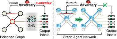
Figure 1: The principle of adversary exploiting the inherent vulnerabilities caused by global optimization to attack GNNs, and the defense mechanism of GAgN against these attacks.

In response to the edge-perturbing attacks, existing defense mechanisms primarily rely on global-optimization-based defense methods [12]. Their objective is to enhance the robustness of GNNs through adversarial training [13], aiming to increase the tolerant ability of perturbations to defend against potential adversarial perturbations. These approaches may still inherit some inherent vulnerabilities of GNNs, as their model frameworks still follow the global-optimization pattern of GNNs. Representative examples include: (1) RGCN [14] replaces the hidden representations of nodes in each graph convolutional network (GCN) [1] layer to the Gaussian distributions, to further absorb the effects of adversarial changes. (2) GCN-SVD [15] combines a singular value decomposition (SVD) filter prior to GCN to eliminate adversarial edges in the training set. (3) STABLE [16] reforms the forward propagation of GCN by adding functions that randomly recover the roughly removed edges. Unfortunately, the computational universality of GNNs has been recently demonstrated [17, 18], signifying that attributed graphs can be classified into any given label space, even those subject to malicious manipulation. This implies that defense approaches focused on enhancing GNNs’ global robustness [14, 15, 16, 19, 20, 21] remain theoretically vulnerable, with potential weaknesses to targeted secondary attacks. In fact, the vulnerability of existing global-optimization-based defenses has been theoretically proven [22]. Adversaries can reduce the classification accuracy of these defenses once again by launching secondary attacks using these defenses as surrogate models. Experimental evidence demonstrates that even under the protection of state-of-the-art defensive measures [23], secondary attacks targeting these defenses successfully mislead 72.8% of the nodes into making incorrect classifications once again.

To overcome the issues mentioned above, inspired by the natural filtering ability of decentralized intelligence [24, 25, 26, 27], we propose a decentralized agent network called Graph Agent Networks (GAgN) whose principle is shown in Fig. 1. GAgN empowers nodes with autonomous awareness, while limiting their perspectives to their 1-hop neighbors. As a result, nodes no longer rely solely on global-level end-to-end training data. Instead, they progressively gain the perception of the entire network through communication with their neighbors and accomplish self-classification. GAgN is designed to enhance the agent-based model (ABM) [28, 29, 30], ensuring improved compatibility with graph-based scenarios. In GAgN, agents are interconnected within the graph topology and engage in cautious communication to mitigate the impact of potential adversarial edges. As time progresses, agents systematically exchange information to broaden their receptive fields, perceive the global information, and attain decentralized intelligence to thus achieve adversarial resilience.

Specifically, GAgN initialize a graph as an agent network where each agent is endowed with three principal abilities:

• Storage, which encompasses states representing both the agent’s and 1-hop neighbors’ current features, actions that serve as parameters for inference functions, and the agent’s own label.

• Inference, which enables an agent to perform global reasoning tasks based on its stored inference functions. These tasks include computing its own embedding, estimating the potential degree of a given node, and determining the neighboring confidence between two specific nodes. The first function equips GAgN with the ability to perform node classification, while the latter two jointly contribute to filtering adversarial edges.

• Communicate, which enables agents to receive and integrate the states and actions of their 1-hop neighbors to augment their own inferential abilities.

Following this, GAgN instigates communication between agents, initially premised on zero trust. During a communication round, each agent acquires training data received from its neighboring agents through predefined I/O interfaces. These data are then organized into a mini-dataset under a limited view, which is employed to train the agent’s inference function, thereby accomplishing agent-level inference tasks. To generalize this inferential capacity to arbitrary node in the graph, each agent further assimilates inference function parameters from neighboring agents into its own inference function. This integration allows agents for global inference capabilities at the graph-level, even under restricted views.

Finally, after a sufficiently prolonged period of communication (i.e., upon the convergence of the inference function’s loss), GAgN opens new communication channels for agents that adhere to the I/O interface specifications. This prompts mutual inspection among agents to identify and filter out suspect adversarial edges using their well-trained functions.

We demonstrate that GAgN and GraphSAGE [2], currently the most potent GNN, are equivalent in terms of their message passing modes. This finding underpins the node classification capability of GAgN. Concurrently, we rigorously prove that all functions in GAgN can be accomplished by the single-hidden-layer multilayer perceptron (MLPs) [31]. In other words, theoretically, within an agent, only three trainable matrices are required in the trainable part, excluding deep-layer networks, bias matrices, and other trainable parameters, to successfully perform the corresponding tasks. This conclusion offers theoretical backing for substantially reducing GAgN’s computational complexity. In practice, by instantiating nodes as lightweight agents, a GAgN can be constructed to carry out node classification tasks with adversarial resilience.

Our main contributions include the following three aspects:

• We propose a decentralized agent network, GAgN, which empowers nodes with the ability to autonomously perceive and utilize global intelligence to address the inherent vulnerabilities of GNNs and existing defense models.

• We theoretically prove that an agent can accomplish the relevant tasks using only three trainable matrices.

• We experimentally show that functions in GAgN are effectively executed, which collectively yielding state-of-the-art classification accuracy in perturbed datasets.

We format the paper as follows: Section II introduces related work. Section III presents the specific technical details of our GAgN. Section IV demonstrates the theoretical results pertinent to GAgN. Section V gives the relevant deployments and results of the experiments. Section VI concludes our work.

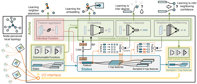
Figure 2: The internal structure and communication paradigm of an agent within GAgN. Initially, the agent organizes a miniature dataset based on received data to train its functions. It then integrates the functions of its neighbors to further expand its receptive field of the global graph. Ultimately, the agent trains functions that possess effective inferential capabilities and self-classification.

II Related works

II-A Edge-perturbing Attacks

Edge-perturbing attacks serve as a primary example of adversarial attacks against GNNs. Through an end-to-end training process, the GNN’s message passing mechanism can be strategically altered to manipulate the classification of the target node or diminish the model’s overall performance. Pioneering works in the realm of adversarial attacks on graph structures were proposed by Dai et al.[32] and Zügner et al.[33], leading to the advent of numerous graph attack methodologies specifically tailored for node prediction tasks. Subsequently, in 2019, Aleksandar et al. [34] conducted the inaugural adversarial vulnerability analysis on the broadly employed methods based on random walks and introduced efficient adversarial perturbations that disrupt the network structure. The following year, Chang et al.[35] launched attacks on diverse graph embedding models using a black-box driven method. Concurrently, Wang et al.[36] designed a threat model to characterize the attack surface of collective classification methods, with a focus on adversarial collective classification. The foundation of these attacks resides in the perturbed graph structure, which is the central subject of this article. Ma et al.[37] explored black-box attacks on GNNs under a novel and realistic constraint where attackers can only access a subset of nodes in the network. Moreover, Xi et al.[38] introduced the first backdoor attack on GNNs, significantly elevating the misclassification rate of popular GNNs on real-world data.

II-B Defenses for Edge-perturbing Attacks

On the defensive front, most protection strategies are typically based on the global-optimization patterns. Zügner et al.[39] were the first to propose a method for certifying robustness (or the lack thereof) of graph convolutional networks with respect to perturbations of the node attributes. Zhu et al.[14] put forward RGCNs designed to automatically neutralize the effects of adversarial changes in the variances of Gaussian distributions. Several defense approaches leverage the concept of generation to bolster the model’s robustness. For instance, Deng et al. [40] presented batch virtual adversarial training (BVAT), a novel regularization method for GCNs that enhances model robustness by incorporating perturbed embeddings. Feng [41] proposed Graph Adversarial Training (GAD), which accounts for the influence from connected examples while learning to construct and resist perturbations. They also introduced an adversarial attack on the standard classification to the graph. Tang et al. [42] researched a novel problem of boosting the robustness of GNNs against poisoning attacks by exploiting a clean graph and generating supervised knowledge to train the model in detecting adversarial edges, thus improving the robustness of GNNs. Liao et al.[43] developed a framework to locally filter out pre-determined sensitive attributes through adversarial training with total variation and the Wasserstein distance, providing robust defense across various graph structures and tasks. Liu et al.[19] proposed Elastic GNNs (EGNN) that can adaptively learn representations of nodes and edges on a graph, dynamically adding or removing nodes and edges to defend against malicious edge perturbations. Jin et al.[21] put forth Pro-GNN, which enhances GNN robustness by optimizing a structural loss function. This measure increases the network’s stability and resilience against attacks targeting nodes and edges.

III The Proposed Method

III-A Preliminaries

We consider connected graphs $\mathcal{G}=(\mathcal{V},\mathcal{E})$ consisting $|\mathcal{V}|$ nodes. The degree of node $v_{i}$ is denoted by $\mathrm{deg}_{i}$. The feature vector and on-hot encoding label of node $v_{i}$ is $\mathbf{z}_{i}\in\mathbb{R}^{1\times d_{z}}$ and $\mathbf{\ell}_{i}\in\mathbb{R}^{1\times d_{L}}$, respectively. The maximum degree over nodes in $\mathcal{G}$ is denoted as $\mathrm{deg}_{\mathrm{max}}$. The edge connected $v_{i}$ and $v_{j}$ is written as $e_{i,j}$ or $e_{j,i}$. The neighborhood $\mathrm{N}_{i}$ of a node $v_{i}$ consists of all nodes $v_{j}$ for which $e_{i,j}\in\mathcal{E}$.

In matrix operations, $\oslash$ operator denotes element-wise division, $\odot$ denotes Hadamard product. $\mathrm{Sum}(\cdot)$ is a function that computes the summation of all elements. By given a set of vectors, $\mathrm{Concat}_{r}(\cdot)$ and $\mathrm{Concat}_{c}(\cdot)$ outputs the concatenated matrix in row-wise and column-wise, respectively. $\mathrm{OneHot}(\cdot)$ converts categorical data into one-hot encoding.

III-B Overview

In GAgN, structures of I/O interfaces, computational models, and storage are same for all agents. Despite these similarities, each agent operates independently, given the distinct information it receives from neighboring agents.

The agent comprises the following components:

• State space that consists of 1) the agent’s and its neighbors’ features, which are communicated through an information exchange mechanism between agents, and 2) inferring results of the degree and the neighbor relationship by given features. Inferring results are typically not computed unless a request for computation is initiated.

• Action spaces that defines the inferring functions, which including individual and communicable functions.

• I/O interface that serves as a conduit for data exchange between agents and their neighbors. It defines the types of information that can be exchanged including states and communicable functions.

• Decision rules that retrieve the parameters of action spaces based on the agent’s current state.

• Action update rules that aggregate neighboring agents’ actions to update the agent’s itself actions.

Figure 2 illustrates the internal structure and communication paradigm of an agent within GAgN. The state of each agent primarily consists of features utilized for inference and the corresponding inference results, with their format predominantly determined by other inference components. Thus, we initiate our discussion with action spaces, and intersperse the introduction of the state’s structure and update strategies while elaborating on other components, aiming to clearly elucidate the entire process.

III-C Action Spaces

The action space comprises the set of all potential actions that a node can undertake in a given reasoning task [44]. In GAgN, the action space is devised as a series of perception functions, sharing identical parameter structures but different specific parameters. The optimal function parameters of agents for each communication round can be found within the action space. Below, we use node $v_{i}$ as an example to expound on these functions it encompasses.

III-C1 Individual Function

Parameters of individual function are agent-specific, reflecting the understanding they gain through interactions with their neighbors, without necessitating direct agent interactions. This includes:

$\blacktriangleright$ Neighbor feature aggregator $\mathcal{A}_{i}:\mathbb{R}^{(\text{deg}_{i}+1)\times d_{z}}\to\mathbb{R}^{d_{z}}$ that aggregate features from $v_{i}$’s local neighborhood into $v_{i}$ itself. Notably, similar to graph attention network (GAT) [3], the features of the nodes themselves are also treated as neighbors for aggregation. The trainable parameter of $\mathcal{A}_{i}$ is an attention vector $\mathbf{w}_{i}\in\mathbb{R}^{\text{deg}_{i}+1}$ that preserves the attention between $v_{i}$ and its neighbors. $\mathcal{A}_{i}$ aggregate features of $\mathrm{N}_{i}$ as

$$\mathcal{A}_{i}(\mathrm{N}_{i})=\frac{\mathbf{w}_{i}\mathrm{Concat}_{r}(\{\mathbf{z}_{i}\}\cup\{\mathbf{z}_{j}:v_{j}\in\mathrm{N}_{i}\})}{\mathrm{deg}_{i}+1}.$$ (1)

Here $\mathbf{w}_{i}$ is initialized to a vector with the smallest possible values, and it is updated iteratively when node $v_{i}$ receives information.

III-C2 Communicable Functions

Parameters of communicable functions are exchangeable, allowing agents to broaden their collective perception through sharing. By communicating, agents can learn from others’ perceptions and integrate this knowledge into their own understanding. These functions encompass:

$\blacktriangleright$ Embedding function $\mathcal{M}_{i}:\mathbb{R}^{1\times d_{z}}\to\mathbb{R}^{1\times d_{L}}$ that embeds node features into the label space. We have proved that an effective embedding can be generated using a $d_{z}\times d_{L}$-dimensional trainable matrix (see Corollary 1).

$\blacktriangleright$ Degree inference function $\mathcal{D}_{i}:\mathbb{R}^{1\times d_{z}}\to\mathbb{R}^{1\times\mathrm{deg}_{\mathrm{max}}}$ that predicts the probability distribution of a node’s degree across the range of 1 to $\mathrm{deg}_{\mathrm{max}}$ (i.e., one-hot encoding) using a given feature. Instantiating $\mathcal{D}_{i}$ as a a $d_{z}\times\mathrm{deg}_{\mathrm{max}}$-dimensional trainable matrix can provide sufficient capacity for fitting (see Theorem 2).

$\blacktriangleright$ Neighboring confidence function $\mathcal{N}_{i}:\mathbb{R}^{1\times 2d_{z}}\to\mathbb{R}$, a binary-classifier that infers whether two given node features are ground-truth neighbors, and the conclusion is provided in the form of a confidence value. We have proved that any two nodes on $\mathcal{G}$ can be inferred neighborhood relationship by a $2d_{z}\times 1$-dimensional trainable matrix (see Theorem 3).

Notably, while intuitive perception suggests that $\mathcal{D}_{i}$ and $\mathcal{N}_{i}$ can be effectively trained end-to-end, this is infeasible in GAgN due to potential adversaries exist and agents’ limited view, restricting access to ample global training samples.

III-D I/O Interface

The internal structure of a node supports its input and output functionality.

III-D1 Input

In a single communication round, node $v_{i}$ receives the following messages from its neighbors $\mathrm{N}_{i}$. 1) Communicable functions of all nodes in $\mathrm{N}_{i}$, i.e., sets of functions $\mathcal{M}_{i}^{\mathrm{rec}}=\{\mathcal{M}_{j}:v_{j}\in\mathrm{N}_{i}\}$, $\mathcal{D}_{i}^{\mathrm{rec}}=\{\mathcal{D}_{j}:v_{j}\in\mathrm{N}_{i}\}$, and $\mathcal{N}_{i}^{\mathrm{rec}}=\{\mathcal{N}_{j}:v_{j}\in\mathrm{N}_{i}\}$. 2) Features from the 1-hop neighbors $Z^{\mathrm{I}}_{i}=\{\mathbf{z}_{j}:v_{j}\in\mathrm{N}_{i}\}$. 3) Sampled features from the 2-hop neighbors $Z^{\mathrm{II}}_{i}=\bigcup_{v_{j}\in\mathrm{N}_{i}}\mathrm{S}(v_{j})-Z^{\mathrm{I}}_{i}$, where $\mathrm{S}(\cdot)$ denotes the sample function. Note that second-order neighbor features are transmitted through immediate neighbors, so the sampling $\mathrm{S}(\cdot)$ occurs when the corresponding first-order neighbor sends messages out.

III-D2 Output

Node $v_{i}$ sends the following messages to its neighbors $\mathrm{N}_{i}$. 1) Feature in the current communication round $\mathbf{z}_{i}$. 2) Sampled features from node $v_{i}$’s neighbor. In this approach, $v_{i}$ samples (i.e., operates $\mathrm{S}(\cdot)$) from its received immediate neighbor features $Z^{\mathrm{I}}$ and sends them out. The sampling function of $v_{i}$ aims to sample the neighbors’ features that have a relatively large difference from its own feature. That is, for a specific receiving nodes $v_{k}$, this approach reduces the similarity between the $Z^{\mathrm{I}}_{k}$ and $Z^{\mathrm{II}}_{k}$, while reducing the amount of messages transmitted outward. Therefore, given the sampling size $\rho$, $\mathrm{S}(\cdot)$ is defined as

$$\mathrm{S}(v_{i})=\left\{\begin{array}[]{l}\mathrm{N}_{i},\rho\leq|\mathrm{N}_{i}|\\ \{\mathbf{z}_{j}:v_{j}\in{N}_{i},\mathrm{rank}(||\mathbf{z}_{j},\mathbf{z}_{i}||_{2})\leq\rho\},\rho>|\mathrm{N}_{i}|\end{array}\right.,$$ (2)

where $\mathrm{rank}(\cdot)$ denotes the rank, i.e., a smaller rank indicating a larger value. 3) Communicable functions $\mathcal{M}_{i}$, $\mathcal{D}_{i}$, and $\mathcal{N}_{i}$.

III-E Decision Rules

The decision rules dictate the mechanism for choosing the corresponding action in different states [45, 46]. In GAgN, the decision rules are specified as the mechanism for training parameters of the functions in the action space, which is based on $v_{i}$’s states after receiving messages from its neighbors. These functions compute the adjustment direction for their parameters through the loss function and obtain trained parameters using stochastic gradient descent (SGD). Next, we introduce these loss-based rules separately.

III-E1 Decision Rule of $\mathcal{A}_{i}$

The loss function $J_{\mathcal{A}}(\cdot)$ of $\mathcal{A}_{i}$ encourages to assign different weights to the neighbors of $v_{i}$, with the aim of obtaining a more accurate embedding that is closer to its label. Therefore, given a aggregated feature $\mathbf{z}^{\mathcal{A}}_{i}=\mathcal{A}_{i}(\mathrm{N}_{i})$, based on the cross-entropy loss,

$$J_{\mathcal{A}}(z^{\mathcal{A}}_{i})=-\log\mathcal{M}_{i}(\mathbf{z}^{\mathcal{A}}_{i})\mathbf{\ell}_{i}^{\top}.$$ (3)

Then, the parameters of $\mathcal{A}_{i}$ can be updated through stochastic gradient descent based backpropagation. It should be noted that although $\mathcal{M}_{i}$ is involved in the computation during the forward propagation, the parameter updates for $\mathcal{A}_{i}$ and $\mathcal{M}_{i}$ are asynchronous. This is due to synchronous updates would result in agents’ private understanding (i.e., $\mathcal{A}_{i}$’s parameters) leaking to their neighborhood before communication through end-to-end training. Thus, the gradient used to update $\mathcal{A}_{i}$ is

$$\nabla_{\mathcal{A}_{i}}^{\mathrm{update}}=\nabla_{\mathcal{A}_{i}}\left(J_{\mathcal{A}}(\mathbf{z}^{\mathcal{A}}_{i})\right).$$ (4)

To obtain $\nabla_{\mathcal{A}_{i}}^{\mathrm{update}}$, we perform iterative training while freezing the parameters of $\mathcal{M}_{i}$.

III-E2 Decision Rule of $\mathcal{M}_{i}$

During training, parameters of $\mathcal{A}_{i}$ are frozen before updating the parameters of $\mathcal{M}_{i}$, i.e.,

$$\nabla_{\mathcal{M}_{i}}^{\mathrm{update}}=\nabla_{\mathcal{M}_{i}}\left(J_{\mathcal{A}}(\mathbf{z}^{\mathcal{A}}_{i})\right).$$ (5)

$\mathcal{A}_{i}$ and $\mathcal{M}_{i}$ share the same forward propagation process. Upon explicit request for specific tasks, i.e., when the training of the corresponding model parameters is initiated, $\mathcal{A}_{i}$ and $\mathcal{M}_{i}$ independently perform back propagation based on $J_{\mathcal{A}}(z^{\mathcal{A}}_{i})$, thus maintaining the non-communicability of $\mathcal{A}_{i}$. This concept is illustrated in Fig. 3.

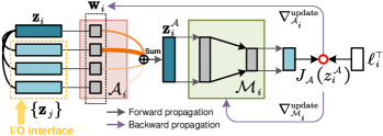
Figure 3: Independent training flow of $\mathcal{A}_{i}$ and $\mathcal{M}_{i}$ with the same forward propagation.

III-E3 Decision Rule of $\mathcal{D}_{i}$

Through the I/O interface, agents obtain their neighbors’ features and their corresponding degrees. Based on this information, the aim of $\mathcal{D}_{i}$ is to learn the relationship between features and degrees from the agent’s limited perspective. In the training phase, the true degrees of neighbors are provided as one-hot encoding to supervise the parameter updates of $\mathcal{D}_{i}$. This implies that the features can be mapped to discrete probability distributions of varying degrees by $\mathcal{D}_{i}$. Furthermore, the agent will allocate weights to the loss corresponding to different neighbors based on the attention vector $W_{i}$, in order to reduce the weight of the loss provided by neighbors with lower attention.

We denote the matrix representation of $\mathcal{D}_{i}$’s inference as

$$\mathcal{X}_{i}^{\mathcal{D}}=\sigma(\mathrm{Concat}_{r}(\mathcal{D}_{i}(\{\mathbf{z}_{j}:v_{j}\in\mathrm{N}_{i}\}\cup\mathbf{z}_{i}))),$$ (6)

where $\sigma$ is the nonlinear activation function, and the concatenated one-hot vector that encodes $v_{i}$’s and its neighbors’ degrees as the supervisor:

$$\mathcal{Y}^{\mathcal{D}}_{i}=\mathrm{OneHot}(\{d_{j}:v_{j}\in\mathrm{N}_{i}\}\cup\mathrm{deg}_{i}).$$ (7)

Then, the loss function of $\mathcal{D}_{i}$ is defined as a Kullback-Leibler divergence weighted by neighbor attention, i.e.,

$$J_{\mathcal{D}}(\mathcal{X}_{i}^{\mathcal{D}})=-\frac{\mathrm{Sum}\left(\mathcal{X}_{i}^{\mathcal{D}}\log\left(\mathcal{X}_{i}^{\mathcal{D}}\oslash\mathcal{Y}^{\mathcal{D}}_{i}\right)\mathbf{I}\odot\mathbf{w}_{i}\right)}{\mathrm{deg}_{i}+1},$$ (8)

where $\mathbf{I}$ is an all-ones vector with $\mathrm{deg}_{\mathrm{max}}$ items that serves to assist in computing the sum of the elements in each row of a matrix.

III-E4 Decision Rule of $\mathcal{N}_{i}$

$v_{i}$ employs $\mathcal{N}_{i}$ to determine whether two nodes have a neighboring relationship based on their features. The training data for $\mathcal{N}_{i}$ is sourced from the sets of features within the scope of $v_{i}$’s view, i.e., $\mathbf{z}_{i}$ and $\{\mathbf{z}_{j}:v_{j}\in\mathrm{N}_{i}\}$. In a graph, the distinguishable decision region exists for the similarity patterns between $v_{i}$ with its first-order and second-order neighbors [47, 48]. Therefore, $\mathcal{N}_{i}$ solely relies on the samples received in the current communication round, to accomplish the binary classification training task between 2 categories: 1) the feature pairs that are labeled as “neighbor” with training samples

$$\mathcal{X}^{\mathcal{N}}_{1}=\{\mathrm{Concat}_{c}(\mathbf{z}_{i},\mathbf{z}_{j}),\mathrm{Concat}_{c}(\mathbf{z}_{j},\mathbf{z}_{i}):v_{j}\in Z^{\mathrm{I}}_{i}\},$$ (9)

and 2) the feature pairs that are labeled as “non-neighbor” with training samples

$$\mathcal{X}^{\mathcal{N}}_{0}=\{\mathrm{Concat}_{c}(\mathbf{z}_{i},\mathbf{z}_{k}),\mathrm{Concat}_{c}(\mathbf{z}_{k},\mathbf{z}_{i}):v_{k}\in Z^{\mathrm{II}}_{i}\}.$$ (10)

Then, according to the training samples $\mathcal{X}^{\mathcal{N}}=\mathcal{X}^{\mathcal{N}}_{1}\cup\mathcal{X}^{\mathcal{N}}_{0}$, the loss function of $\mathcal{D}_{i}$ is defined as the binary cross-entropy loss, i.e.,

$$\small J_{\mathcal{N}}(\mathcal{X}^{\mathcal{N}})=-\frac{\sum_{x_{l}\in\mathcal{X}^{\mathcal{N}}_{1}}\log\left(\mathcal{N}_{i}(x_{l})\right)}{|\mathcal{X}^{\mathcal{N}}_{1}|}-\frac{\sum_{x_{l}\in\mathcal{X}^{\mathcal{N}}_{0}}\left(1-\log\left(\mathcal{N}_{i}(x_{l})\right)\right)}{|\mathcal{X}^{\mathcal{N}}_{0}|}.$$ (11)

All loss functions are differentiable, enabling diverse functions to undergo self-training based on their associated losses. By employing SGD for parameter adjustment, these functions progressively converge the loss, thereby enhancing their inference capabilities.

III-F Action Update Rules

This section introduces action update rules, which play a crucial role in updating the actions of agents based on the actions (i.e., functions) received from their neighbors. By employing these rules, agents can dynamically adjust their actions to better adapt to the evolving environment and improve their collective performance.

In accordance with the previous discussion, we consider node $v_{i}$ as a case in point. From the perspective of an individual vertex $v_{i}$, it obtains the integrated feature of its neighbors’ actions in the current round by weighted fusion of the transmitted actions from its neighbors. Based on this synthesized feature, $v_{i}$ updates its own actions accordingly. The weighted fusion methods are elaborated in the following subsections.

III-F1 Action Update Rule of $\mathcal{M}_{i}$

The embedding function directly impacts the classification results which the adversaries target at, and any node in $\mathcal{V}$ could potentially be compromised (i.e., some neighbors of $v_{i}$ might be malicious). Therefore, $v_{i}$ cannot fully trust its neighbors’ embedding functions. Considering that the attention weights are individual functions, immune to the accumulation of malicious messages through iterative training, the weighted fusion of $\mathcal{M}_{i}^{\mathrm{rec}}$ using $\mathbf{w}_{i}$ can help filter out some harmful gradients, allowing for a benign update of $\mathcal{M}_{i}$. Specifically, the parameter of $\mathcal{M}_{i}$ is updated as

$$\bm{\theta}_{\mathcal{M}_{i}}\leftarrow\bm{\theta}_{\mathcal{M}_{i}}+\eta_{\mathcal{M}}\frac{\omega_{i,j}\sum_{\mathcal{M}_{j}\in\mathcal{M}_{i}^{\mathrm{rec}}}\left(\bm{\theta}_{\mathcal{M}_{j}}-\bm{\theta}_{\mathcal{M}_{i}}\right)}{|\mathrm{N}_{i}|},$$ (12)

where $\omega_{i,j}$ is the $j$-th attention in $\mathbf{w_{i}}$ and $\eta_{\mathcal{M}}$ is the learning rate for updates that is usually the same as that for $\mathcal{M}_{i}$ itself.

III-F2 Action Update Rule of $\mathcal{D}_{i}$

For the same feature, different degree inference functions may output different inference results. Therefore, $v_{i}$ aims to train a middleware function $\mathscr{D}_{i}$ such that the inference results for $\mathbf{z}_{k},\forall v_{k}\in\mathcal{V}$ derived from $\mathscr{D}_{i}$ are as similar as possible to those from recieved functions (i.e., the set $\mathcal{D}_{i}^{\mathrm{rec}}$). To address this, we randomly initialize $\mathscr{D}_{i}$ and design a loss function based on spatial random sampling to train $\mathscr{D}_{i}$, guiding the fusion of stored functions and the update of $\mathcal{D}_{i}$. Specifically, we perform the following steps: 1) Carry out small-scale random perturbations in the Euclidean space to sample features $\mathbf{z}_{s}$ similar to $\mathbf{z}_{i}$, which is calculated by $\mathbf{z}_{s}=\mathbf{z}_{i}+\xi\mathbf{x}$ where $\mathbf{x}$ is an i.i.d. 0-1 random vector that satisfies Gaussian distribution, $\xi$ is the sample range, thereby increasing the number of samples. 2) Utilize the features of nodes in $Z^{\mathrm{II}}_{i}$ as negative samples to enhance sample diversity from a limited perspective. 3) Employ $\mathscr{D}_{i}$ and $\mathcal{D}_{i}^{\mathrm{rec}}$ to infer these samples separately and use the mean squared error (MSE) to quantify the discrepancy between the inference results. The training strategy for $\mathscr{D}_{i}$ is illustrated in Fig. 4.

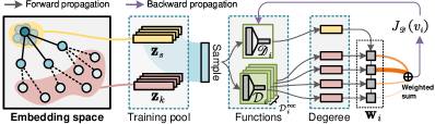
Figure 4: The training strategy for $\mathscr{D}_{i}$.

In summary, the loss function of $\mathscr{D}_{i}$ is

$$J_{\mathscr{D}}(v_{i})=\sum_{\mathcal{D}_{j}\in\mathcal{D}_{i}^{\mathrm{rec}}}\omega_{i,j}\Big{[}-\sum_{Q}{\mathbb{E}}_{\mathbf{z}_{s}\sim P\left(\mathbf{z}_{i}\right)}{\mathrm{MSE}\left(\mathscr{D}_{i}(\mathbf{z}_{s}),\mathcal{D}_{j}(\mathbf{z}_{s})\right)}\\ -\sum_{v_{k}\in Z^{\mathrm{II}}_{i}}{\mathrm{MSE}\left(\mathscr{D}_{i}(\mathbf{z}_{k}),\mathcal{D}_{j}(\mathbf{z}_{k})\right)}\Big{]},$$ (13)

where $P$ is a sampling distribution in the Euclidean space, $Q$ defines the number of sample, and $\mathrm{MSE}(\cdot)$ is the MSE function. After training that employing $J_{\mathscr{D}}(v_{i})$ as the loss, the parameter of $\mathcal{D}_{i}$ is updated as

$$\bm{\theta}_{\mathcal{D}_{i}}\leftarrow\bm{\theta}_{\mathcal{D}_{i}}+\eta_{\mathcal{D}}\left(\bm{\theta}_{\mathcal{D}_{i}}-\bm{\theta}_{\mathscr{D}_{i}}\right),$$ (14)

where $\bm{\theta}_{\mathscr{D}_{i}}$ is the parameter of the well-trained $\mathscr{D}_{i}$.

III-F3 Action Update Rule of $\mathcal{N}_{i}$

From Eqs. (9) and (10), it can be observed that under a limited view, the training set consistently encompasses $z_{i}$ when training $\mathcal{N}_{i}$ for any node $v_{i}$. This suggests that $\mathcal{N}_{i}$ can only determine whether a neighboring relationship exists between itself and a node with a given feature, rather than generalizing this inferential ability to arbitrary pairs of nodes. The action update mechanism presents an opportunity for such generalization. By receiving the neighboring functions $\mathcal{N}_{i}^{\mathrm{rec}}$ through the I/O interface, these functions enable the expansion of $\mathcal{N}_{i}$’s receptive field on a richer dataset, allowing $\mathcal{N}_{i}$ to learn the inferential capabilities of its neighbors.

Specifically, we perform the following steps: 1) Construct a training set using the same method as in Eqs. (9) and (10). 2) Both $\mathcal{N}_{i}$ and $\mathcal{N}_{i}^{\mathrm{rec}}$ are utilized to predict the output of the same training samples simultaneously. 3) For a specific neighbor $v_{k}$, the output of $\mathcal{N}_{k}$ serves as a metric to evaluate the similarity between the inferential ability of $\mathcal{N}_{i}$ and $\mathcal{N}_{k}$. If they are similar, it indicates that $\mathcal{N}_{i}$’s inferential ability on the sample aligns with $\mathcal{N}_{k}$, and substantial adjustments are not required. On the contrary, if they differ, a larger loss value is returned, compelling $\mathcal{N}_{i}$ to adjust its parameters to approach the corresponding $\mathcal{N}_{k}$. 4) Through iterative training, all received $\mathcal{N}_{i}^{\mathrm{rec}}$ are involved in evaluating $\mathcal{N}_{i}$, leading to the completion of function fusion.

The evaluation result of $\mathcal{N}_{k}$ for $\mathcal{N}_{i}$ is quantified using the absolute values between the outputs. After all functions in $\mathcal{D}_{i}^{\mathrm{rec}}$ have provided their evaluations, the loss is calculated by weighted summation according to the aforementioned method, which in turn is used to compute the required gradient updates for a single round update of $\mathcal{N}_{i}$:

$$\small\bm{\theta}_{\mathcal{N}_{i}}\leftarrow\bm{\theta}_{\mathcal{N}_{i}}-\eta_{\mathcal{N}}\frac{\partial\sum_{x_{k}\in\mathcal{X}^{\mathcal{N}}_{0}\cup\mathcal{X}^{\mathcal{N}}_{1}}\sum_{\mathcal{N}_{j}\in\mathcal{N}_{i}^{\mathrm{rec}}}\omega_{i,j}\left|\mathcal{N}_{i}(x_{k})-\mathcal{N}_{j}(x_{k})\right|}{\mathrm{deg}_{i}|\mathcal{X}^{\mathcal{N}}_{0}\cup\mathcal{X}^{\mathcal{N}}_{1}|\partial\bm{\theta}_{\mathcal{N}_{i}}}.$$ (15)

Through multiple rounds of training, the collective guidance of $\mathcal{N}_{j},\forall v_{j}\in\mathrm{N}_{i}$ on $\mathcal{N}_{i}$’s gradient descent direction is achieved through continuous evaluations, progressively fusing their inferential abilities into $\mathcal{N}_{i}$.

III-G Filtering Adversarial Edges

As communication between agents tends towards convergence, they initiate the detection of adversarial edges. Given that all agents possess the capacity for inference, an intuitive approach would be to allow inter-agent detection until a sufficient and effective number of adversarial edges are identified. However, this method necessitates the execution of $|\mathcal{V}|\times|\mathcal{V}|$ inference calculations, the majority of which are redundant and do not proportionately contribute to the global detection rate relative to the computational power consumed. Therefore, we propose a multilevel filtering method that significantly reduces computational load while preserving a high detection rate.

Specifically, the entire detection process is grounded in the functions trained from the agents’ first-person perspectives, with each agent acting both as a detector and a detectee. The detection procedure consists of four steps, illustrated by taking node $v_{i}$ as the detector and node $v_{x}$ as the detectee:

• For any node $v_{x}$, if there is a neighbor with insufficient attention, the edge formed by this neighbor relationship is considered as a suspicious edge.

• Random proxy communication channels are established, introducing an unfamiliar neighbor $v_{i}$ to $v_{x}$, with both parties exchanging information through I/O interfaces.

• $v_{i}$ infers the degree of $v_{x}$ based on its own experience (i.e., applies $\mathcal{D}_{i}(\mathbf{z}_{x})$); if the inferred result deviates from the actual outcome, the process advances to the subsequent detection step; otherwise, a new detectee is selected.

• $v_{i}$ estimates neighbor confidence between $v_{x}$ and its neighbors using its experience (i.e., computing $\mathrm{Concat}_{c}(\mathbf{z}_{x},\mathbf{z}_{u})$, $\forall v_{u}\in\mathrm{N}_{x}$); edges with trust levels below a threshold are identified as adversarial edges.

Employing this approach, administrators possessing global model access rights are limited to establishing proxy connections, which entails creating new I/O interfaces for nodes without the ability to interfere in specific message passing interactions between them. As a result, distributed agents are responsible for conducting detection tasks, enabling individual intelligences to identify adversarial perturbations derived from global training.

IV Theoretical Analysis

In this section, we present the theoretical foundations for the design of inference function structures within agents and demonstrate their computational universality for the target tasks. Firstly, we establish the global equivalence between GAgN and GraphSAGE.

Theorem 1 (Equivalence).

Denote $\mathbb{M}(\mathcal{G})=\{\mathbf{z}^{\mathbb{M}}_{i}=\mathcal{M}_{i}(\mathbf{z}_{i}):v_{i}\in\mathcal{V}\}$ as the global embedding result of all nodes, and $\texttt{SAGE}(\mathcal{G})=\{\mathbf{z}^{\texttt{S}}_{i},...\mathbf{z}^{\texttt{S}}_{|\mathcal{V}|}\}$ as the global classification result of GraphSAGE. For any SAGE there exists $\mathbb{M}$ that

$$\mathbb{M}(\mathcal{G})=\texttt{SAGE}(\mathcal{G}),\forall\mathcal{G}\in G,$$ (16)

where $G$ is the set of all attributed graphs.

Proof.

First, we demonstrate that the first-order message passing of $\mathbb{M}$ and SAGE is equivalent (meaning that the depth of SAGE is 1). This equivalence arises from the diverse calculation methods for SAGE, which depend on the selection of its aggregator. By examining different instantiations of $\mathcal{A}$ and $\mathcal{M}$, we establish their respective equivalences.

GraphSAGE [2] that employs mean aggregator updates the feature (i.e., a single round of forward propagation) as

$$\mathbf{z}_{i}^{\texttt{S}}=\sigma\left(\mathbf{W}^{1}_{\texttt{S}}\cdot\mathrm{Mean}(\{\mathbf{z}_{i}\}\cup\{\mathbf{z}_{\mathrm{N}_{i}}\})\right),$$ (17)

where $\{\mathbf{z}_{\mathrm{N}_{i}}\}=\{{\mathbf{z}_{j}:v_{j}\in\mathrm{N}_{i}}\}$ is the neighboring feature set, $\mathbf{W}^{1}_{\texttt{S}}$ is the weight matrix of 1-hop neighborhood, $\mathrm{MEAN}(\cdot)$ is the mean operator. It is not difficult to see that by instantiating $\mathbf{w}_{i}$ as an all-ones vector $\mathbf{I}^{\prime}$ with $\mathrm{deg}_{i}+1$ items, $\mathcal{A}_{i}$ can thus aggregate features as

$$\small\mathcal{A}_{i}(\mathrm{N}_{i}) =\frac{\mathbf{I}^{\prime}\mathrm{Concat}_{r}(\{\mathbf{z}_{i}\}\cup\{\mathbf{z}_{\mathrm{N}_{i}}\})}{\mathrm{deg}_{i}+1}=\frac{\mathrm{Sum}(\{\mathbf{z}_{i}\}\cup\{\mathbf{z}_{\mathrm{N}_{i}}\})}{\mathrm{deg}_{i}+1}$$

$$=\mathrm{Mean}(\{\mathbf{z}_{i}\}\cup\{\mathbf{z}_{\mathrm{N}_{i}}\}).$$ (18)

Then, by instantiating $\mathcal{M}_{i}$ as a function that computes the output by left-multiplying the input with a trainable matrix $\mathbf{W}_{\mathbb{M}}$ and the nonlinear activation (i.e., instantiated as a fully-connected neural network), we have

$$\mathbf{z}^{\mathbb{M}}_{i}=\mathcal{M}_{i}(\mathcal{A}_{i}(\mathrm{N}_{i}))=\sigma\left(\mathbf{W}_{\mathbb{M}}\cdot\mathrm{Mean}(\{\mathbf{z}_{i}\}\cup\{\mathbf{z}_{\mathrm{N}_{i}}\})\right).$$ (19)

Eqs. (17) and (19) respectively represent the computation processes of 1-depth mean-aggregator SAGE and $\mathbb{M}$, when their trainable matrix have same shape, i.e., $\mathbf{W}_{\mathbb{M}}\sim\mathbf{W}^{1}_{\texttt{S}}$, their equivalence can be apparently observed. In our discussion concerning the embedding results at the agent level, it is worth noting that we will no longer employ subscript $i$ to differentiate trainable matrices $\mathbf{W}_{\mathbb{M}}$. It is crucial to recognize that $\mathbf{W}_{\mathbb{M}}$ does not represent a global model, and this notation is solely utilized to demonstrate the aforementioned theory.

GraphSAGE that employed mean-pooling aggregator updates the feature as

$$\mathbf{z}_{i}^{\texttt{S}}=\sigma\left(\mathbf{W}^{1}_{\texttt{S}}\cdot\mathrm{MeanPool}\left(\{\sigma\left(\mathbf{z}_{i},\mathbf{z}_{j}\mathbf{W}_{\texttt{P}}+\mathbf{b}\right),\forall v_{j}\in\mathrm{N}_{i}\}\right)\right),$$ (20)

where $\mathbf{W}_{\texttt{P}}$ is a fully-connected neural network in pooling aggregator, $\mathbf{b}$ is the bias vector. Next, we instantiate $\omega_{i,j}$ as

$$\omega_{i,j}=\left\{\begin{array}[]{ l }1+\mathbf{b}\mathbf{W}_{\mathbb{M}}^{-1}\mathbf{z}_{j}^{+},i\neq j\\ \mathbf{z}_{i}\mathbf{W}_{\mathbb{M}}^{-1}\mathbf{z}_{i}^{+},i=j\end{array}\right.,$$ (21)

where $\mathbf{z}_{j}^{+}\in\mathbb{R}^{d_{z}}$ is the pseudoinverse of $\mathbf{z}_{j}$. Then, we instantiate $\mathcal{M}_{i}$ as a 2-layer neural network (with trainable matrix $\mathbf{W}_{\mathbb{M}}$ and $\mathbf{W}^{\prime}_{\mathbb{M}}$) and a pooling layer whose forward propagation is formulated as

$$\mathcal{M}(\mathbf{x})=\sigma\left(\mathbf{W}^{\prime}_{\mathbb{M}}\cdot\frac{\sigma\left(\mathbf{x}\mathbf{W}_{\mathbb{M}}\right)}{|\mathrm{N}_{i}+1|}\right).$$ (22)

$\mathcal{M}_{i}$ can therefore embed features as

$$\mathbf{z}^{\mathbb{M}}_{i} =\mathcal{M}_{i}(\mathcal{A}_{i}(\mathrm{N}_{i}))$$

$$=\sigma\left(\mathbf{W}^{\prime}_{\mathbb{M}}\cdot\frac{\sigma\left(\left(\omega_{i,i}\mathbf{z}_{i}+\sum_{v_{j}\in\mathrm{N}_{i}}\omega_{i,j}\mathbf{z}_{j}\right)\mathbf{W}_{\mathbb{M}}\right)}{|\mathrm{N}_{i}+1|}\right).$$ (23)

Since

$$(\omega_{i,i}\mathbf{z}_{i} +\sum_{v_{j}\in\mathrm{N}_{i}}\omega_{i,j}\mathbf{z}_{j})\mathbf{W}_{\mathbb{M}}=\omega_{i,i}\mathbf{z}_{i}\mathbf{W}_{\mathbb{M}}+\sum_{v_{j}\in\mathrm{N}_{i}}\omega_{i,j}\mathbf{z}_{j}\mathbf{W}_{\mathbb{M}}$$

$$=\mathbf{z}_{i}\mathbf{W}_{\mathbb{M}}^{-1}\mathbf{z}_{i}^{+}\mathbf{z}_{i}\mathbf{W}_{\mathbb{M}}+\sum_{v_{j}\in\mathrm{N}_{i}}\left(1+\mathbf{b}\mathbf{W}_{\mathbb{M}}^{-1}\mathbf{z}_{j}^{+}\right)\mathbf{z}_{j}\mathbf{W}_{\mathbb{M}}$$

$$=\mathbf{z}_{i}+\sum_{v_{j}\in\mathrm{N}_{i}}\left(\mathbf{z}_{j}\mathbf{W}_{\mathbb{M}}+\mathbf{b}\mathbf{W}_{\mathbb{M}}^{-1}\mathbf{z}_{j}^{+}\mathbf{z}_{j}\mathbf{W}_{\mathbb{M}}\right)$$

$$=\mathbf{z}_{i}+\sum_{v_{j}\in\mathrm{N}_{i}}\mathbf{z}_{j}{\mathbf{W}_{\mathbb{M}}}+\mathbf{b},$$ (24)

substituting Eq. (IV) into Eq. (IV) yields:

$$\mathbf{z}^{\mathbb{M}}_{i} =\mathcal{M}_{i}(\mathcal{A}_{i}(\mathrm{N}_{i}))$$

$$=\sigma\left(\mathbf{W}^{\prime}_{\mathbb{M}}\cdot\frac{\sigma\left(\mathbf{z}_{i}+\sum_{v_{j}\in\mathrm{N}_{i}}{\mathbf{z}_{j}\mathbf{W}_{\mathbb{M}}}+\mathbf{b}\right)}{|\mathrm{N}_{i}+1|}\right)$$ (25)

$$=\sigma\left(\mathbf{W}^{\prime}_{\mathbb{M}}\cdot\mathrm{MeanPool}\left(\sigma\left(\{\mathbf{z}_{i},\mathbf{z}_{j}\mathbf{W}_{\mathbb{M}}+\mathbf{b}\}:v_{j}\in\mathrm{N}_{i}\right)\right)\right).$$

Eqs. (IV) and (20) respectively represent the computation processes of $\mathbb{M}$ and 1-depth pool-aggregator SAGE. $\mathcal{M}_{i}$ enables the shape of its trainable matrices to be identical to that of $\mathbf{W}^{1}_{\texttt{S}}$ and $\mathbf{W}_{\texttt{P}}$, i.e., $\mathbf{W}^{\prime}_{\mathbb{M}}\sim\mathbf{W}^{1}_{\texttt{S}}$ and $\mathbf{W}_{\mathbb{M}}\sim\mathbf{W}_{\texttt{P}}$, leading to the equivalence between the two entities, as their computational patterns align.

The aforementioned analysis demonstrates that GAgN and GraphSAGE are equivalent in the context of 1-depth aggregation. Building upon this conclusion, we will now establish the equivalence of GAgN and GraphSAGE in the case of $K$-depth aggregation as well. We denote a single aggregation in GraphSAGE as $\mathrm{AGG}_{1}(\cdot)$, then the 1-depth aggregation is formulated as

$$\mathbf{z}_{i}^{\texttt{S},K=1}=\sigma\left(\mathbf{W}^{1}_{\texttt{S}}\mathrm{A{\scriptstyle GG}}_{1}(\mathrm{N}_{i})\right).$$ (26)

The 2-depth aggregation is

$$\mathbf{z}_{i}^{\texttt{S},K=2} =\sigma\left(\mathbf{W}^{2}_{\texttt{S}}\mathrm{A{\scriptstyle GG}}_{1}(\{\mathbf{z}_{j}^{\texttt{S},K=1}:v_{j}\in\mathrm{N}_{i}\})\right)$$

$$=\sigma\left(\mathbf{W}^{1}_{\texttt{S}}\mathrm{A{\scriptstyle GG}}_{1}(\left\{\sigma\left(\mathbf{W}^{2}_{\texttt{S}}\mathrm{A{\scriptstyle GG}}_{1}(\mathrm{N}_{i})\right)\right\}:v_{j}\in\mathrm{N}_{i}\})\right).$$ (27)

We write Eq. (IV) as $\mathbf{z}_{i}^{\texttt{S},K=2}=\mathrm{A{\scriptstyle GG}}_{2}(\mathrm{N}_{i})$. From Eqs (26) and (IV), it can be observed that $\mathrm{A{\scriptstyle GG}}_{2}(\mathrm{N}_{i})$ is a deep nested function [49] based on $\mathrm{A{\scriptstyle GG}}_{1}(\mathrm{N}_{i})$. The nesting rule involves $\mathrm{A{\scriptstyle GG}}_{2}(\mathrm{N}_{i})$ taking the output of $\mathrm{A{\scriptstyle GG}}_{1}(\mathrm{N}_{i})$ as input, re-entering it into $\mathrm{A{\scriptstyle GG}}_{1}(\mathrm{N}_{i})$, and replacing the parameter $\mathbf{W}^{1}_{\texttt{S}}$ in $\mathrm{A{\scriptstyle GG}}_{1}(\mathrm{N}_{i})$ with $\mathbf{W}^{2}_{\texttt{S}}$. We denote this nested rules as

$$\mathrm{A{\scriptstyle GG}}_{2}(x)=\left(\mathrm{A{\scriptstyle GG}}_{1}^{\mathbf{W}^{1}_{\texttt{S}}}\circ\mathrm{A{\scriptstyle GG}}_{1}^{\mathbf{W}^{2}_{\texttt{S}}}\right)(x),$$ (28)

where $\mathrm{A{\scriptstyle GG}}_{1}^{\mathbf{W}^{1}_{\texttt{S}}}$ denotes the $\mathrm{A{\scriptstyle GG}}_{1}$ with the parameter $\mathbf{W}^{1}_{\texttt{S}}$.

Consequently, given an argument $x$, we can write

$$\mathrm{A{\scriptstyle GG}}_{K}(x)=\left(\mathrm{A{\scriptstyle GG}}_{1}^{\mathbf{W}^{1}_{\texttt{S}}}\circ\ldots\circ\mathrm{A{\scriptstyle GG}}_{1}^{\mathbf{W}^{K}_{\texttt{S}}}\right)(x).$$ (29)

It is evident that if a set of nested functions $F=\{F_{1},\ldots,F_{K}\}$ satisfies

• its initial nesting functions is equivalent to $\mathrm{A{\scriptstyle GG}}_{1}$, and

• its nesting rules are identical with Eq (29),

then $F_{K}$ is equivalent to $\mathrm{A{\scriptstyle GG}}_{K}$.

During the $e$-th communication round of GAgN, node $v_{j}$ trains its models $\mathcal{M}_{j}$ and $\mathcal{A}_{j}$ via the data received from the I/O interface, thus learning the features of its 1-hop neighbors. We denote $\mathrm{L{\scriptstyle EARN}}^{j}_{1}(\cdot)$ as the learning function of $v_{j}$ within a single communication round. Then, we can write

$$\mathbf{z}^{\mathbb{M},e}_{j}=\mathcal{M}_{j}\left(\mathcal{A}_{j}\left(\mathrm{N}_{j}\right)\right)=\mathrm{L{\scriptstyle EARN}}^{j}_{1}(\mathrm{N}_{j}).$$ (30)

Subsequently, we shift our focus to any neighboring node $v_{i}$ of $v_{j}$. In the ($e$+1)-th communication round, $v_{i}$ learns the feature of $v_{j}$ by

$$\mathbf{z}^{\mathbb{M},e+1}_{i}=\mathrm{L{\scriptstyle EARN}}^{i}_{1}\left(\left\{\mathrm{L{\scriptstyle EARN}}^{j}_{1}\left(\mathrm{N}_{j}\right):v_{j}\in\mathrm{N}_{i}\right\}\right).$$ (31)

At this point, $v_{j}$ has already integrated the features of its 1-hop neighbors during the $e$-th communication round, and a portion of these neighbors are 2-hop neighbors of $v_{i}$. Consequently, after 2 communication rounds, $v_{i}$’s receptive field expands to include its 2-hop neighbors. The learning from 2-hop neighbors is formulated as $\mathbf{z}^{\mathbb{M},e}_{j}=\mathrm{L{\scriptstyle EARN}}^{j}_{2}(\mathrm{N}_{j})$. From Eqs. (30) and (31), it is evident that $\mathrm{L{\scriptstyle EARN}}$ is also a nested function, with the nested rule being:

$$\small\mathrm{L{\scriptstyle EARN}}^{j}_{K}(x)=\underbrace{\left(\mathrm{L{\scriptstyle EARN}}^{j}_{1}\circ\mathrm{L{\scriptstyle EARN}}^{i}_{1}\circ\ldots\circ\mathrm{L{\scriptstyle EARN}}_{1}^{j_{K}}\right)}_{K\text{ items}},\normalsize$$ (32)

where $v_{j_{K}}$ is the arbitrary K-hop neighbor of $v_{j}$. The equivalence of and $\mathbb{M}$ and 1-depth aggregation supports that $\mathrm{L{\scriptstyle EARN}}^{j}_{1}=\mathrm{A{\scriptstyle GG}}_{1}$. Further, since the agents enables the shape of its trainable matrices to be identical to that of $\{\mathbf{W}^{1}_{\texttt{S}},\ldots,\mathbf{W}^{K}_{\texttt{S}}\}$, we can deduce that the nested rule of the learning function of GAgN (formulated as Eq. (32)) and the aggregator in GraphSAGE (formulated as Eq. (29)) are equivalent. Consequently, the equivalence between $\mathbb{M}$ and $K$-depth pool-aggregator SAGE is thus established. ∎

Subsequently, we propose the following corollaries to guide the design of the embedding function:

Corollary 1.

Given that model $\mathcal{M}_{i}$ is instantiated as a single-layer neural network, with its trainable parameters represented by a $d_{z}\times d_{L}$-dimensional matrix, it can be asserted that $\mathbb{M}_{i}$ is computationally universal for the task of embedding any arbitrary feature space onto the corresponding label space.

Proof.

Suppose there exists a Turing-complete function $\mathcal{T}$, capable of performing precise node-level classification. Thanks to the theory of GNN Turing completeness [17], i.e., a GNN that has enough layers is Turing complete, which can be formulated as: $\mathrm{A{\scriptstyle GG}}_{\infty}=\mathcal{T}$. Based on the conclusions derived from Theorem 1, we have that the sufficiently communicated function $\mathrm{L{\scriptstyle EARN}}_{\infty}$ is equivalent to $\mathrm{A{\scriptstyle GG}}_{\infty}$. The computational accessibility of M for embedding tasks can thus be demonstrated by the transitive equivalence chain $\mathcal{M}_{i}=\mathrm{L{\scriptstyle EARN}}_{\infty}=\mathrm{A{\scriptstyle GG}}_{\infty}=\mathcal{T}$. ∎

Regarding the structure of the degree inference function, we arrive at the following conclusions:

Theorem 2.

Given any attribute graph $\mathcal{G}$, it can be definitively mapped from its associated feature matrix to any specified label matrix by employing a single linear transformation (i.e., a trainable matrix) and applying a nonlinear activation.

Proof.

First, we derive the characteristics of an effective one-hot degree matrix for a graph. According to the Erdos-Gallai theorem [50], if an $N\times\mathrm{deg}_{\mathrm{max}}$-dimensional degree matrix $\hat{\mathbf{L}}$ satisfies the following condition:

$$\sum_{i=1}^{r}\underset{j}{\arg\max\hat{\mathbf{L}}{i,j}}\leq r(r-1)+\sum_{i=r+1}^{N}\min(r,\underset{j}{\arg\max\hat{\mathbf{L}}_{i,j}}),$$ (33)

then a valid graph can be constructed based on the degrees represented by $\hat{\mathbf{L}}$. Here, we consider a more generalized scenario. Suppose there is a degree set without a topological structure, i.e., the corresponding one-hot degree matrix, denoted as $\mathbf{L}$ , is not subject to the constraint of Eq. (33). If there exists a matrix $\mathbf{W}$ capable of fitting any 0-1 matrix $\mathbf{L}$, i.e.,

$$\mathrm{MSE}(\sigma(\mathbf{Z}\mathbf{W}),\mathbf{L})<\epsilon,\forall\epsilon>0,$$ (34)

then it is considered that $\mathbf{W}$ can fit arbitrary degree matrices. As a corollary, since the feasible domain of $\hat{\mathbf{L}}$ is a subdomain of $\mathbf{L}$, the above theory can be proven. Subsequently, by introducing Eq. (33) as a regularization term to guide the convergence direction of $\mathbf{W}$, $\hat{\mathbf{L}}$ can be obtained.

In order to prove the solvability of $\mathbf{W}$ in Eq. (34), intuitively, it can be solved by solving matrix equation. However, since $\mathbf{Z}$ is typically row full rank [51], the rank of $\mathbf{Z}^{\top}\mathbf{Z}$ is not equal to $d_{z}$, which implies that the pseudoinverse of $\mathbf{Z}$ can only be approximately obtained, and thus the existence of a solution to the matrix equation cannot be proven directly. To address this, we use the Moore-Penrose (MP) pseudoinverse [52] to approximate the pseudoinverse of $\mathbf{Z}$. By conducting singular value decomposition on $\mathbf{Z}$, we obtain $\mathbf{Z}=\mathbf{U}\mathbf{D}\mathbf{V}^{\top}$, where $\mathbf{U}$ and $\mathbf{V}$ are invertible matrices and $\mathbf{D}$ is the singular value matrix. The MP pseudoinverse of $\mathbf{Z}$ is solvable and given by $\mathbf{Z}^{\dagger}=\mathbf{V}\mathbf{D}^{+}\mathbf{U}^{\top}$.

According to Tikhonov Regularization [53], $\mathbf{Z}^{\dagger}=\lim_{\alpha\to 0}\mathbf{Z}^{\top}(\mathbf{Z}\mathbf{Z}^{\top}+\alpha\Upsilon)^{-1}$ where $\Upsilon$ the identity matrix. We can apply the Taylor series expansion method from matrix calculus. In this case, we expand $(\mathbf{Z}\mathbf{Z}^{\top}+\alpha\Upsilon)^{-1}$ with respect to $\alpha$. This can be expressed as:

$$\small\left(\mathbf{Z}\mathbf{Z}^{\top}+\alpha\Upsilon\right)^{-1}\\ =\left(\mathbf{Z}\mathbf{Z}^{\top}\right)^{-1}-\alpha\left(\mathbf{Z}\mathbf{Z}^{\top}\right)^{-1}\Upsilon\left(\mathbf{Z}\mathbf{Z}^{\top}\right)^{-1}+O(\alpha^{2})\\ =\left(\mathbf{Z}\mathbf{Z}^{\top}\right)^{-1}+O(\alpha),$$ (35)

where $O(\cdot)$ denotes the higher-order terms.

Therefore, for any learning target $\mathbf{Z}\mathbf{W}=\mathbf{L}$, there exists a matrix $\mathbf{W}=\mathbf{V}\mathbf{D}^{+}\mathbf{U}^{\top}\mathbf{L}$, such that

$$\mathbf{Z}\mathbf{W} =\mathbf{Z}\lim_{\alpha\to 0}\left(\left(\mathbf{Z}^{\top}\left(\mathbf{Z}\mathbf{Z}^{\top}\right)^{-1}+O\left(\alpha\right)\right)\right)\mathbf{L}$$

$$=\lim_{\alpha\to 0}\left(\left(\mathbf{Z}\mathbf{Z}^{\top}\left(\mathbf{Z}\mathbf{Z}^{\top}\right)^{-1}\mathbf{L}+\mathbf{Z}O(\alpha)\mathbf{L}\right)\right)$$

$$=\lim_{\alpha\to 0}\left(\mathbf{L}+O(\alpha)\right),$$ (36)

and the output loss can thus be expressed as:

$$\small\mathrm{MSE}(\sigma(\mathbf{Z}\mathbf{W}),\mathbf{L})=\mathrm{MSE}\left(\sigma\left(\lim_{\alpha\to 0}(\mathbf{L}+O(\alpha))\right),\mathbf{L}\right)<\epsilon.\normalsize$$ (37)

The solvability of $\mathbf{W}$ as presented in Eq. (34) is supported by Eq. (37), which demonstrates that $\mathbf{W}$ can be fitted to any given degree matrix. ∎

For the neighboring confidence function’s structure, we present the following findings:

Theorem 3.

For a graph $\mathcal{G}$ with arbitrary edge distribution, there exists a solvable and fixed $2d_{z}$-dimensional weight vector $\mathbf{q}=[q_{1},\ldots,q_{2d_{z}}]$, such that for any two nodes $v_{i}$ and $v_{j}$ within $\mathcal{G}$ and their true neighboring relationship $\phi$ (where $\phi$ is a relative minimum or a value that converges to 1), $\mathrm{Concat}_{r}(\mathbf{z}_{i},\mathbf{z}_{j})\mathbf{q}^{\top}=\phi$ is solvable.

Proof.

First, we define two equivalent normed linear spaces, $A\sim\mathbb{R}^{d_{z}}$ and $B\sim\mathbb{R}^{d_{z}}$. The graph $\mathcal{G}$ can be mapped into these spaces. Specifically, the node features are represented as points in spaces $A$ and $B$, while the edge distribution of $\mathcal{G}$ can be characterized as corresponding relationships between these two spaces. In this way, $\mathcal{G}$ is mapped into two spaces with corresponding relationships.

Next, we define diagonal matrices $\mathbf{D}_{A}=\mathrm{diag}(q_{1},\ldots q_{d_{z}})$ and $\mathbf{D}_{B}=\mathrm{diag}(q_{d_{z}+1},\ldots q_{2d_{z}})$ for linear transformations, which, in the form of left multiplication of coordinates, scale the coordinates of vectors in spaces $A$ and $B$ across different dimensions to varying degrees. Since dimensions are mutually independent in the phenomenon space, solvable $\mathbf{D}_{A}$ and $\mathbf{D}_{B}$ exist to realize the mutual mapping of equivalent spaces.

Subsequently, we arbitrarily assign a value to $\phi$ and randomly divide it into two parts, such that $\phi$ = $\phi_{1}$ + $\phi_{2}$. We then define an equivalent space $C$ to $A$ and $B$, and sample two points with row-vector coordinates $\mathbf{c}_{1}$ and $\mathbf{c}_{2}$ in $C$ that satisfy $||\mathbf{c}_{1}||_{1}=\phi_{1}$ and $||\mathbf{c}_{2}||_{1}=\phi_{2}$.

Now, based on the above conditions, we arbitrarily sample two points from $A$ and $B$, with row-vector coordinates $\mathbf{a}$ and $\mathbf{b}$, representing any two nodes in $\mathcal{G}$. Considering the randomness of edge distribution, $\phi$ can characterize the random neighbor relationship between them. We map $\mathbf{a}$ and $\mathbf{b}$ to space $C$ using $\mathbf{D}_{A}$ and $\mathbf{D}_{B}$, i.e., $\mathbf{c}_{1}=\mathbf{D}_{A}\mathbf{a}$, $\mathbf{c}_{2}=\mathbf{D}_{B}\mathbf{b}$. Thus, we obtain:

$$\mathrm{Concat}_{c}(\mathbf{a},\mathbf{b})[q_{1},q_{2},\ldots,q_{2d_{z}}]^{\top}=||\mathbf{D}_{A}\mathbf{a}+\mathbf{D}_{B}\mathbf{b}||_{1}\\ =||\mathbf{D}_{A}\mathbf{a}||_{1}+||\mathbf{D}_{B}\mathbf{b}||_{1}=||\mathbf{c}_{1}||_{1}+||\mathbf{c}_{2}||_{1}=\phi_{1}+\phi_{2}=\phi.$$ (38)

As evidenced by Eq.(38), $\mathrm{Concat}_{r}(\mathbf{z}_{i},\mathbf{z}_{j})\mathbf{q}^{\top}=\phi$ holds. ∎

V Experiments

V-A Experimental Settings

Datasets. Our approaches are evaluated on six real-world datasets widely used for studying graph adversarial attacks [54, 22, 14, 15, 16], including Cora, Citeseer, Polblogs, and Pubmed.

Baselines. Our proposed GAgN can protect non-defense GNNs against edge-perturbing attacks, meanwhile outperforming other defense models. Specifically, baselines include:

Comparison defending models. We compare GAgN with other defending models including: 1) RGCN which leverages the Gaussian distributions for node representations to amortize the effects of adversarial attacks, 2) GNN-SVD which is applied to a low-rank approximation of the adjacency matrix obtained by truncated SVD, 3) Pro-GNN [21] which can learn a robust GNN by intrinsic properties of nodes, 4) Jaccard [20] which defends attacks based on the measured Jaccard similarity score, 5) EGNN [19] which filters out perturbations by $l_{1}$- and $l_{2}$-based graph smoothing.

Attack methods. The experiments are designed under the following attack strategies: 1) Metattack, a meta-learning based attack, 2) G-EPA [22], the general edge-perturbing attack.

In this paper, unless specified, the perturbation rate for attacks is set to 20%, which is the value commonly adopted in most literature.

V-B Classification Accuracy

Here we assess the global classification accuracy of our proposed GAgN in the context of both primary and secondary attacks. Our experimental setup employs GCN and corresponding defenses as surrogate models for Metattack and G-EPA, given that Metattack is the strongest primary attack and G-EPA is an effective secondary attack approach. We replicated each set of settings ten times and documented the mean values and the range of variation classification accuracy. These results are reported in Table I. The best data is marked in bold, while the second best data is underlined. Note that since our proposed GAgN does not have global input-output interfaces, we cannot directly use it as a surrogate model to perform secondary attacks. To account for this, we transfer different perturbed graphs generated on the baselines with secondary attacks to the GAgN test set. We conduct five sets of experiments, reporting the average accuracy and variation range to demonstrate GAgN’s accuracy under secondary attacks. In our setup, the diversity of the baselines ensures that the test set already encompasses almost all potential inherent vulnerabilities targeting defenses. If GAgN maintains high accuracy under this test set, it suggests that it has eliminated the inherent vulnerabilities of GNNs and can effectively filter out potential adversarial edges. Our results indicate that GAgN achieves the best classification accuracy under both primary and secondary attacks. The significance of this cannot be overstated. Given the absence of global input-output interfaces in GAgN, it presents a considerable challenge for adversaries aiming to exploit its potential vulnerabilities via global training. This characteristic essentially renders GAgN nearly impervious to secondary attacks, thereby reinforcing its adversarial resilience.

TABLE I: Comparison of defense classification (%) accuracy under primary and secondary attack, $r_{p}$ is the perturbation rate.

Surrogate		GCN (primary attack by Metattack)						Corresponding defenses (secondary attack by G-EPA)
	$r_{p}$	RGCN	GNN-SVD	Pro-GNN	Jaccard	EGNN	GAgN	RGCN	GNN-SVD	Pro-GNN	Jaccard	EGNN	GAgN
Cora	0	82.84±0.23	80.89±0.72	84.89±0.19	81.71±0.31	84.12±0.64	85.41±0.16	73.14±0.73	70.39±1.22	75.59±0.69	71.21±0.81	73.62±1.14	82.31±0.66
	5	76.59±0.33	78.29±0.88	79.94±0.10	79.51±1.09	81.37±0.67	83.12±0.32	65.49±0.83	66.79±1.38	68.84±0.60	68.01±2.09	70.27±1.17	79.62±1.02
	10	72.82±0.21	69.98±1.64	74.45±0.11	74.28±1.18	75.81±0.22	79.86±0.13	61.32±0.71	57.38±2.64	63.25±0.61	62.78±2.18	64.71±0.72	75.46±0.63
	20	58.67±0.39	57.01±1.18	63.94±0.61	72.51±0.84	69.02±0.89	77.01±0.24	49.17±0.89	47.91±2.18	55.04±1.11	63.11±1.84	59.52±1.39	74.91±0.74
Citeseer	0	70.43±0.95	69.84±0.60	74.08±0.65	72.98±0.48	74.31±0.92	76.77±0.39	61.93±1.45	61.34±1.10	65.68±1.15	64.48±0.98	65.81±1.42	74.27±0.89
	5	71.15±0.88	68.11±0.76	71.67±1.12	70.64±0.95	73.62±0.62	75.12±0.47	62.65±1.38	59.51±1.26	63.17±1.62	62.14±1.45	64.62±1.12	73.62±0.97
	10	66.94±0.89	68.81±0.68	69.37±1.29	70.03±0.76	73.11±0.58	74.95±0.42	58.44±1.39	60.31±1.18	60.87±1.79	61.53±1.26	65.12±1.08	73.45±0.92
	20	62.53±1.50	57.29±1.27	56.24±1.09	66.21±1.07	64.94±1.44	70.49±0.41	54.03±2.00	48.79±1.77	47.74±1.59	57.71±1.57	56.44±1.94	69.19±0.91
Polblogs	0	95.28±0.29	95.33±0.33	95.96±0.35	94.87±0.71	95.69±0.47	96.61±1.08	86.78±0.79	86.83±0.83	87.46±0.85	86.37±1.21	87.19±0.97	94.11±2.08
	5	73.54±0.30	89.10±0.76	90.59±0.93	90.71±0.83	89.95±1.53	92.83±1.50	65.04±0.80	80.60±1.26	82.09±1.43	82.21±1.33	81.45±2.03	91.33±2.00
	10	70.64±0.45	79.93±0.96	85.35±1.35	85.66±1.64	83.22±2.09	87.86±1.62	62.14±0.95	71.43±1.46	76.85±1.85	77.16±2.14	74.72±2.59	85.36±2.12
	20	58.36±0.67	54.87±2.21	73.10±0.85	69.87±1.57	75.42±1.04	80.92±1.88	49.86±1.17	46.37±2.71	64.60±1.35	61.37±2.07	66.92±1.54	78.42±2.38
Pubmed	0	84.52±0.60	83.28±0.51	84.96±0.17	84.42±0.28	85.83±0.21	85.01±0.21	76.02±1.10	74.78±1.01	76.46±0.67	75.92±0.78	77.33±0.71	85.51±0.71
	5	81.27±0.73	82.80±0.51	82.84±0.20	81.95±0.26	83.42±0.29	83.27±0.33	72.77±1.23	74.30±1.01	74.34±0.70	73.45±0.76	74.92±0.79	80.77±0.83
	10	78.32±0.58	81.88±0.51	82.75±0.17	81.44±0.21	79.36±0.30	83.15±0.28	69.82±1.08	73.38±1.01	74.32±0.67	72.94±0.71	70.86±0.80	78.65±0.78
	20	71.20±0.84	81.24±0.44	82.82±0.25	76.39±0.23	79.06±0.29	82.98±0.17	62.70±1.34	72.74±0.94	74.07±0.75	67.89±0.73	70.56±0.79	78.29±0.67

V-C Effectiveness of Aggregator

V-C1 Symmetry of Attentions

. In a well-trained GAgN, adjacent agents may learn different attentions for the edges connecting them. We consider the learning of attention by the two agents to be effective, along with their neighbor feature aggregators, if they coincidentally learn similar attentions for the edge in question (i.e., $\omega_{i,j}\approx\omega_{i,j}$). To validate this, we first arbitrarily designate the direction of the edges on the graph, defining the attention of any edge $e_{i,j}$ as the attention $\omega_{i,j}$ from the starting node $v_{i}$ to the terminating node $v_{j}$. As a result, we obtain a new graph with reversed attentions for all edges. We then use a line chart to illustrate the forward and reverse attentions of the same edges after learning in the GAgN model. To ensure the smoothness of a certain edge, we sort the forward attention, obtain the sorted edge index, and use this index to find the corresponding reverse attention. This allows us to examine the variation of forward and reverse attentions under the same edge. As shown in Fig. 5, the variations between forward and reverse attentions are almost identical, indicating that adjacent agents coincidentally learn similar attentions. This observation substantiates the effectiveness of the neighbor feature aggregator in the GAgN model.

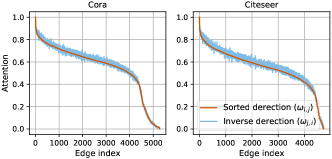
Figure 5: Attentions of random direction and their inverse direction on the same edges.

We further illustrate the fluctuation range of bidirectional attention on the same edge to provide additional evidence for effective communication between agents and to validate the efficacy of the neighbor feature aggregator. We select the node with the largest degree (denoted as $v_{c}$) in the Cora dataset as the central node and observe the forward and reverse attention of the edges formed with its 72 randomly selected neighbors. As shown in Fig. 6, it can be observed that the overall trends of forward and backward attention during the training process are similar, accompanied by tolerable fluctuations, and both converge to approximately the same values.

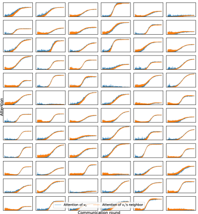
Figure 6: Learning curves of the largest-degree node $v_{c}$ (blue lines) and its neighboring agents (orange lines) for attention on the same edge.

V-C2 Distribution of Attentions

. Here we investigate the attention distribution learned by agents for both normal edges and adversarial edges. A significant distinction between the two would indicate that agents, through communication, have become aware that lower weights should be assigned to adversarial edges, thereby autonomously filtering out information from illegitimate neighbors introduced by such edges. As the previous set of experiments have demonstrated the symmetry of attention, we present the attention of a randomly selected agent on one end of the edge. The experimental results, as depicted in Fig. 7, reveal a notable difference in the kernel density estimation (KDE) of attentions between normal edges and adversarial edges (generated by Metattack). This outcome substantiates that agents, by training the aggregator, have acquired the capability to autonomously filter out adversarial edges.

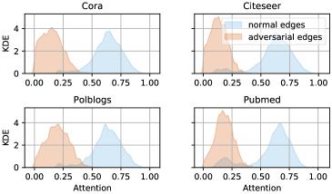
Figure 7: Distribution of attentions on normal and adversarial edges.

V-D Effectiveness of Embedding

Upon completing communication, the agent utilizes a well-trained embedding function to embed its feature into the label space. We conduct a visualization of the global embeddings to investigate whether the agents have acquired effective embeddings. If the agents’ embeddings have not undergone global training and are solely trained based on their own labels under knowledge-limited conditions, yet still exhibit clustering phenomena globally, it demonstrates the effectiveness of the embedding function. Figure 8 displays the embedding of the Cora and Citeseer and visualized by t-SNE [55], where points of different colors represent distinct categories. As can be observed, points from different categories form clear clusters, validating the efficacy of the embedding function.

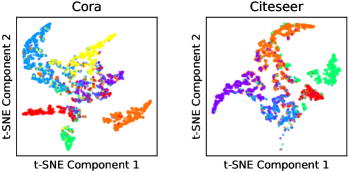
Figure 8: Well-trained agents generated embedding.

Additionally, We provide a detailed account of the training process of node embeddings by GAgN on the Cora dataset. The experimental results are presented in Fig. 9. As can be seen, initially, the embeddings of all nodes are randomly dispersed in the label space. Through communication among agents, the nodes gradually reach a consensus on the embeddings, and by continuously adjusting, they gradually classify themselves correctly and achieve a steady state.

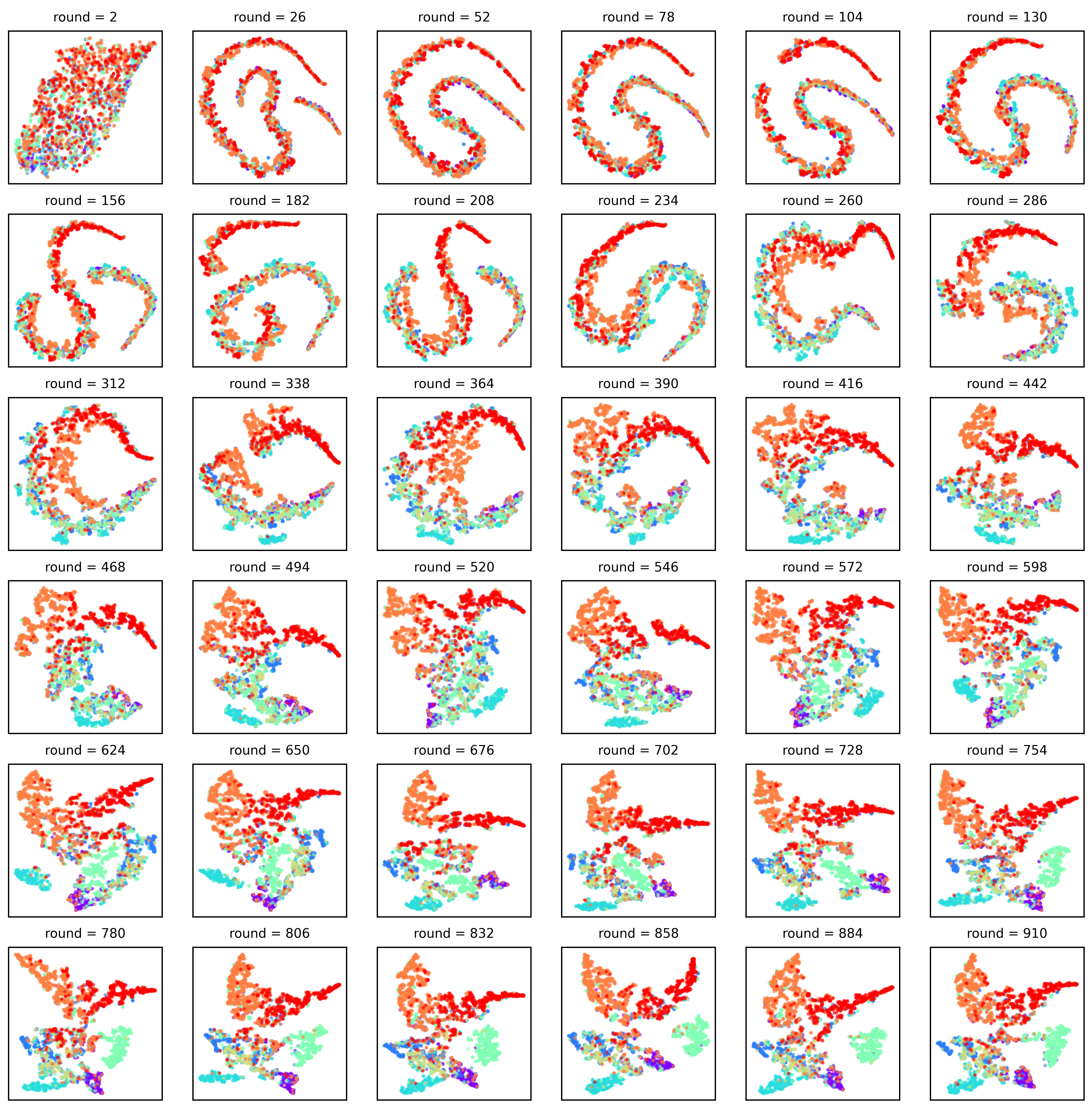
Figure 9: The formation process of embedding in communication rounds.

V-E Effectiveness of Degree Inference

Each agent possesses the ability to infer the degree of any node based on the degree inference function. To validate the effectiveness of this inference, we select 150 representative nodes as test sets after training the GAgN model on the corresponding clean graph, following these rules: 1) the top 50 nodes with the highest degree, denoted as $\{L$-$nodes\}$; 2) the top 50 nodes with the lowest degree, denoted as $\{S$-$nodes\}$; 3) the 50 nodes furthest away from the inference node in terms of graph distance, denoted as $\{D$-$nodes\}$. Notably, to avoid training set leakage into the test set, an agent’s 1-hop neighbors and select 2-hop neighbors are excluded from its test set. The experimental results, as shown in Table II, demonstrate that even without data on the test nodes, agents can generalize their inference capabilities to the nodes of the graph under limited knowledge training, effectively inferring the degree of nodes.

TABLE II: Degree inference accuracy (%)

Test set	$\{L$-$nodes\}$	$\{S$-$nodes\}$	$\{D$-$nodes\}$
Cora	90.35	95.31	92.64
Citeseer	89.21	94.19	91.08
Polblogs	92.41	96.32	92.57

V-F Effectiveness of Neighboring Confidence

To fully validate the effectiveness of the neighboring confidence function on graph $\mathcal{G}$, $|\mathcal{V}\times\mathcal{V}|$ matrix operations are required. In order to reduce the computational complexity while ensuring a fair evaluation process, we construct four representative graphs and utilize the neighbor relationships within these graphs as test samples to create a test set that encompasses potential distinct task attributes: 1) The original graph $\mathcal{G}_{0}$, with test sample labels all set to 1, 2) A graph $\mathcal{G}_{1}$ generated by randomly distributing edges over V, with test sample labels determined by whether the generated edges are original or not, 3) A randomly rewired graph $\mathcal{G}_{2}$, with test sample labels all set to 0, and 4) A graph $\mathcal{G}_{3}$ containing only adversarial edges, with test sample labels all set to 0. Upon constructing the test sets, we randomly select 50 nodes to compute the confidence for neighbor relationships in different test sets, treating this task as a binary classification problem. The classification accuracy represents the effectiveness of the neighboring confidence function. Figure 10 displays the classification accuracy on different test sets constructed within various graphs, demonstrating that the neighboring confidence function achieves satisfactory accuracy in all test sets, thus showcasing its effectiveness.

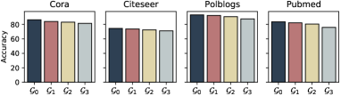
Figure 10: Accuracy of neighboring Confidence function.

V-G Ablation Experiments

We employed a multi-module filtering approach to reduce computational complexity when filtering adversarial edges. To investigate the individual effects of these modules when operating independently, it is crucial to conduct ablation experiments. Section V-C has explored the distribution patterns of attention scores for normal and adversarial edges. Edges with low attention scores are initially considered suspicious, which implies that the attention threshold may influence the detection rate and false alarm rate. To quantitatively examine the impact of threshold selection on these rates, we utilize receiver operating characteristic (ROC) curves. As depicted in Fig. 11, the detection rate is relatively insensitive to the attention threshold. This allows for a high detection rate while maintaining low false alarm rates.

Figure 11: ROC curves with different attention threshold.

TABLE III: Results of ablation experiments

Dataset	Cora		Citeseer
Metrics	TPR	FPR	TPR	FPR
Att.	85.52%	5.56%	82.66%	7.20%
Att.+$\mathcal{D}$+$\mathcal{N}$	83.04%	0.87%	79.60%	1.16%

After identifying suspicious edges based on attention, the degree inference function and neighboring confidence function collaboratively eliminate normal edges from the suspicious ones, further reducing false positive rates. Here we investigate whether these two functions effectively pinpoint adversarial edges while preserving normal edges as much as possible. We utilize true positive rate (TPR) to quantify the detection rate of adversarial edges, and false positive rate (FPR) to measure the misclassification rate of normal edges. We conduct Metattack as the attack method. The experimental results are shown in Table III, where “Att.” denotes detection using only attention, and “Att.+$\mathcal{D}$+$\mathcal{N}$” represents the combined detection of all three methods. It can be observed that solely relying on attention for detection results in a higher detection rate but also introduces a higher false positive rate. By incorporating both the degree inference function and neighboring confidence function, the false positive rate is significantly reduced without substantially affecting the detection rate.

VI Conclusions

In this paper, we proposed GAgN, a novel and effectiveness approach for addressing the inherent vulnerabilities of GNNs to adversarial edge-perturbing attacks. By adopting a decentralized interaction mechanism, GAgN facilitates the filtration of adversarial edges and effectively thwarts global attack strategies. The theoretical sufficiency for GAgN further simplifies the model, while experimental results validate its effectiveness in resisting edge-perturbing attacks compared to existing defenses.

Ao Liu is currently pursuing the Ph.D. degree in School of Cyber Science and Engineering with the Sichuan University, Chengdu, China. His research interests include graph convolutional networks, security and privacy for artificial intelligence, and cybersecurity. He is serving or has served as the reviewer for several journals and conferences, including IEEE TNNLS, Computers & Security, CVPR, ICCV and ECCV.

Wenshan Li received her M.S. degree from University of California, Los Angeles, in 2019. She is currently pursuing the Ph.D. degree in School of Cyber Science and Engineering with the Sichuan University, Chengdu, China. Her current research interests include data science, machine learning and bioinformatics.

Tao Li received the B.S. and M.S. degrees in computer science and the Ph.D. degree in circuit and system from the University of Electronic Science and Technology of China, Chengdu, China, in 1986, 1991, and 1995, respectively. From 1994 to 1995, he was a Visiting Scholar of neural networks theory with the University of California at Berkeley. He is currently a Professor with the College of Cybersecurity, Sichuan University, Chengdu. His current research interests include network security, artificial immune theory, and disaster recovery application.

Beibei Li (S’15–M’19) received the B.E. degree (awarded Outstanding Graduate) in communication engineering from Beijing University of Posts and Telecommunications, P.R. China, in 2014 and the Ph.D. degree (awarded Full Research Scholarship) from the School of Electrical and Electronic Engineering, Nanyang Technological University, Singapore, in 2019. He is currently an associate professor (doctoral advisor) with the School of Cyber Science and Engineering, Sichuan University, P.R. China. He was invited as a visiting researcher at the Faculty of Computer Science, University of New Brunswick, Canada, from March to August 2018, and also the College of Control Science and Engineering, Zhejiang University, P.R. China, from February to April 2019. His current research interests include several areas in security and privacy issues on cyber-physical systems, with a focus on intrusion detection techniques, artificial intelligence, and applied cryptography. He won the Best Paper Award in 2021 IEEE Symposium on Computers and Communications (ISCC). Dr. Li is serving or has served as a Publicity Chair, Publication Co-Chair, or TPC member for several international conferences, including AAAI 2021, IEEE ICC 2021, IEEE ATC 2021, IEEE GLOBECOM 2020, etc.

Hanyuan Huang received the M.S. degree in information and communication engineering from Beijing University of Posts and Telecommunications, China in 2019. She is currently pursuing the Ph.D. degree with the School of Cyber Science and Engineering, Sichuan University, China. Her main research interests include cybersecurity, evolutionary computation, and artificial immune systems.

Guangquan Xu is a Ph.D. and full professor at the Tianjin Key Laboratory of Advanced Networking (TANK), College of Intelligence and Computing, Tianjin University, China. He is also a joint-professor of School of Big Data, Huanghai University, Qingdao. He received his Ph.D. degree from Tianjin University in March 2008. He is an IET Fellow, members of the CCF and IEEE. He is the director of Network Security Joint Lab and the Network Attack & Defense Joint Lab. He has published 100+ papers in reputable international journals and conferences, including IEEE TIFS, IEEE TDSC, JSAC, IEEE TII, IoT J, FGCS, IEEE Communications Magazine, Information Sciences, IEEE Wireless Communications, IEEE Transactions on Cybernetics, ACM TIST, IEEE Network and so on. He served as a TPC member for FCS2020, ICA3PP2021, IEEE UIC 2018, SPNCE2019, IEEE UIC2015, IEEE ICECCS 2014, and reviewers for IEEE Access, ACM TIST, JPDC, IEEE TITS, soft computing, FGCS, and Computational Intelligence, and so on. His research interests include cybersecurity and trust management.

Zhou Pan (S’07–M’14-SM’20) is currently a full professor and PhD advisor with Hubei Engineering Research Center on Big Data Security, School of Cyber Science and Engineering, Huazhong University of Science and Technology (HUST), Wuhan, P.R. China. He received his Ph.D. in the School of Electrical and Computer Engineering at the Georgia Institute of Technology (Georgia Tech) in 2011, Atlanta, USA. He received his B.S. degree in the Advanced Class of HUST, and a M.S. degree in the Department of Electronics and Information Engineering from HUST, Wuhan, China, in 2006 and 2008, respectively. He held honorary degree in his bachelor and merit research award of HUST in his master study. He was a senior technical member at Oracle Inc., America, during 2011 to 2013, and worked on Hadoop and distributed storage system for big data analytics at Oracle Cloud Platform. He received the “Rising Star in Science and Technology of HUST” in 2017, and the “Best Scientific Paper Award” in the 25th International Conference on Pattern Recognition (ICPR 2020). He is currently an associate editor of IEEE Transactions on Network Science and Engineering.

References

- [1] T. N. Kipf and M. Welling, “Semi-supervised classification with graph convolutional networks,” in Proc. 5th Int. Conf. Learn. Represent., 2017.
- [2] W. Hamilton, Z. Ying, and J. Leskovec, “Inductive representation learning on large graphs,” in Proc. 31st Adv. Neural Inf. Proces. Syst., 2017.
- [3] P. Veličković, G. Cucurull, A. Casanova, A. Romero, P. Lio, and Y. Bengio, “Graph attention networks,” in Proc. 5th Int. Conf. Learn. Represent., 2017.
- [4] W. Chen, F. Feng, Q. Wang, X. He, C. Song, G. Ling, and Y. Zhang, “Catgcn: Graph convolutional networks with categorical node features,” IEEE Trans. Knowl. Data Eng., 2021.
- [5] S. Nadal, A. Abelló, O. Romero, S. Vansummeren, and P. Vassiliadis, “Graph-driven federated data management,” IEEE Trans. Knowl. Data Eng., vol. 35, no. 1, pp. 509–520, 2021.
- [6] Y. Zhao, H. Zhou, A. Zhang, R. Xie, Q. Li, and F. Zhuang, “Connecting embeddings based on multiplex relational graph attention networks for knowledge graph entity typing,” IEEE Trans. Knowl. Data Eng., 2022.
- [7] D. Berberidis and G. B. Giannakis, “Node embedding with adaptive similarities for scalable learning over graphs,” IEEE Trans. Knowl. Data Eng., vol. 33, no. 2, pp. 637–650, 2019.
- [8] H. Xiao, Y. Chen, and X. Shi, “Knowledge graph embedding based on multi-view clustering framework,” IEEE Trans. Knowl. Data Eng., vol. 33, no. 2, pp. 585–596, 2019.
- [9] S. Kreps and D. Kriner, “Model uncertainty, political contestation, and public trust in science: Evidence from the COVID-19 pandemic,” Sci. Adv., vol. 6, no. 43, p. eabd4563, Oct. 2020.
- [10] W. Walt, C. Jack, and T. Christof, “Adversarial explanations for understanding image classification decisions and improved neural network robustness,” Nat. Mach. Intell., vol. 1, pp. 508––516, Nov. 2019.
- [11] F. Samuel, G, B. John, D, I. Joichi, Z. Jonathan, L, B. Andrew, L, and K. Isaac, S, “Adversarial attacks on medical machine learning,” Science, vol. 363, no. 6433, pp. 1287–1289, Mar. 2019.
- [12] L. Sun, Y. Dou, C. Yang, K. Zhang, J. Wang, S. Y. Philip, L. He, and B. Li, “Adversarial attack and defense on graph data: A survey,” IEEE Trans. Knowl. Data Eng., 2022.
- [13] F. Feng, X. He, J. Tang, and T.-S. Chua, “Graph adversarial training: Dynamically regularizing based on graph structure,” IEEE Trans. Knowl. Data. Eng., vol. 33, no. 6, pp. 2493–2504, 2019.
- [14] D. Zhu, Z. Zhang, P. Cui, and W. Zhu, “Robust graph convolutional networks against adversarial attacks,” in Proc. 25th ACM SIGKDD Int. Conf. Knowl. Discov. Data Min., Aug. 2019, pp. 1399–1407.
- [15] N. Entezari, S. A. Al-Sayouri, A. Darvishzadeh, and E. E. Papalexakis, “All you need is low (rank) defending against adversarial attacks on graphs,” in Proc. 13th Int. Conf. Web Search Data Min., 2020, pp. 169–177.
- [16] K. Li, Y. Liu, X. Ao, J. Chi, J. Feng, H. Yang, and Q. He, “Reliable representations make a stronger defender: Unsupervised structure refinement for robust gnn,” in Proc. 28th ACM SIGKDD Int. Conf. Knowl. Discov. Data Min., 2022.
- [17] A. Loukas, “What graph neural networks cannot learn: depth vs width,” in Proc. 7th Int. Conf. Learn. Represent., May 2019.
- [18] K. Xu, W. Hu, J. Leskovec, and S. Jegelka, “How powerful are graph neural networks?” in Proc. 7th Int. Conf. Learn. Represent., 2019.
- [19] X. Liu, W. Jin, Y. Ma, Y. Li, H. Liu, Y. Wang, M. Yan, and J. Tang, “Elastic graph neural networks,” in Proc. 38th Int. Conf. Mach. Learn., 2021, pp. 6837–6849.
- [20] H. Wu, C. Wang, Y. Tyshetskiy, A. Docherty, K. Lu, and L. Zhu, “Adversarial examples for graph data: deep insights into attack and defense,” in Proc. 28th Int. Joint Conf. Artif. Intel., 2019.
- [21] W. Jin, Y. Ma, X. Liu, X. Tang, S. Wang, and J. Tang, “Graph structure learning for robust graph neural networks,” in 26th ACM SIGKDD Int. Conf. Knowl. Discov. Data Min., 2020, pp. 66–74.
- [22] A. Liu, B. Li, T. Li, P. Zhou, and R. Wang, “An-gcn: An anonymous graph convolutional network against edge-perturbing attacks,” IEEE Trans. Neural Netw. Learn. Syst., 2022.
- [23] S. Geisler, D. Zügner, and S. Günnemann, “Reliable graph neural networks via robust aggregation,” in Proc. 34th Adv. Neural Inf. Proces. Syst., 2020, pp. 13 272–13 284.
- [24] S. Warnat-Herresthal, H. Schultze, K. L. Shastry, S. Manamohan, S. Mukherjee, V. Garg, R. Sarveswara, K. Händler, P. Pickkers, N. A. Aziz et al., “Swarm learning for decentralized and confidential clinical machine learning,” Nature, vol. 594, no. 7862, pp. 265–270, 2021.
- [25] N. C. Luong, D. T. Hoang, S. Gong, D. Niyato, P. Wang, Y.-C. Liang, and D. I. Kim, “Applications of deep reinforcement learning in communications and networking: A survey,” IEEE Commun. Surv. Tutor., vol. 21, no. 4, pp. 3133–3174, 2019.
- [26] Z. Wang, M. Song, Z. Zhang, Y. Song, Q. Wang, and H. Qi, “Beyond inferring class representatives: User-level privacy leakage from federated learning,” in Proc. IEEE Infocom., 2019, pp. 2512–2520.
- [27] O. L. Saldanha, P. Quirke, N. P. West, J. A. James, M. B. Loughrey, H. I. Grabsch, M. Salto-Tellez, E. Alwers, D. Cifci, N. Ghaffari Laleh et al., “Swarm learning for decentralized artificial intelligence in cancer histopathology,” Nat. Med., vol. 28, no. 6, pp. 1232–1239, 2022.
- [28] S. C. Bankes, “Agent-based modeling: A revolution?” Proc. Natl. Acad. Sci. U.S.A., vol. 99, no. suppl_3, pp. 7199–7200, 2002.
- [29] A. Khodabandelu and J. Park, “Agent-based modeling and simulation in construction,” Autom. Constr., vol. 131, p. 103882, 2021.
- [30] K. M. Carley, D. B. Fridsma, E. Casman, A. Yahja, N. Altman, L.-C. Chen, B. Kaminsky, and D. Nave, “Biowar: scalable agent-based model of bioattacks,” IEEE Trans. Syst. Man Cybern. Syst., vol. 36, no. 2, pp. 252–265, 2006.
- [31] I. O. Tolstikhin, N. Houlsby, A. Kolesnikov, L. Beyer, X. Zhai, T. Unterthiner, J. Yung, A. Steiner, D. Keysers, J. Uszkoreit et al., “Mlp-mixer: An all-mlp architecture for vision,” in Proc. 35th Adv. Neural Inf. Proces. Syst., vol. 34, 2021, pp. 24 261–24 272.
- [32] H. Dai, H. Li, T. Tian, X. Huang, L. Wang, J. Zhu, and L. Song, “Adversarial attack on graph structured data,” in Proc. 35th Int. Conf. Mach. Learn., Jul. 2018, pp. 1115–1124.
- [33] D. Zügner, A. Akbarnejad, and S. Günnemann, “Adversarial attacks on neural networks for graph data,” in Proc. 24th ACM SIGKDD Int. Conf. Knowl. Discov. Data Min., Jul. 2018, pp. 2847–2856.
- [34] A. Bojchevski and S. Günnemann, “Adversarial attacks on node embeddings via graph poisoning,” in Proc. 36th Int. Conf. Mach. Learn., Jun. 2019, pp. 695–704.
- [35] H. Chang, Y. Rong, T. Xu, W. Huang, H. Zhang, P. Cui, W. Zhu, and J. Huang, “A restricted black-box adversarial framework towards attacking graph embedding models,” in Proc. 34th AAAI Conf. Artif. Intell., vol. 34, no. 04, Feb. 2020, pp. 3389–3396.
- [36] B. Wang and N. Z. Gong, “Attacking graph-based classification via manipulating the graph structure,” in Proc. 26th ACM Conf. Computer. Commun. Secur., Nov. 2019, pp. 2023–2040.
- [37] J. Ma, S. Ding, and Q. Mei, “Towards more practical adversarial attacks on graph neural networks,” in Proc. 34th Adv. Neural Inf. Proces. Syst., Dec. 2020.
- [38] X. Zhaohan, P. Ren, J. Shouling, and W. Ting, “Graph backdoor,” in Proc. 29th USENIX Secur. Symp., Aug. 2021.
- [39] D. Zügner and S. Günnemann, “Certifiable robustness and robust training for graph convolutional networks,” in Proc. 25th ACM SIGKDD Int. Conf. Knowl. Discov. Data Min., Aug. 2019, pp. 246–256.
- [40] Z. Deng, Y. Dong, and J. Zhu, “Batch virtual adversarial training for graph convolutional networks,” arXiv preprint arxiv:1902.09192, 2019.
- [41] F. Feng, X. He, J. Tang, and T.-S. Chua, “Graph adversarial training: Dynamically regularizing based on graph structure,” IEEE Trans. Knowl. Data Eng., vol. 33, no. 6, pp. 2493–2504, Jun. 2021.
- [42] X. Tang, Y. Li, Y. Sun, H. Yao, P. Mitra, and S. Wang, “Transferring robustness for graph neural network against poisoning attacks,” in Proc. 13th ACM Int. Conf. Web Search Data Min., Nov. 2020, pp. 600–608.
- [43] L. Peiyuan, Z. Han, X. Keyulu, J. Tommi, G. Geoffrey, J. Stefanie, and S. Ruslan, “Information obfuscation of graph neural networks,” Proc. 38th Int. Conf. Mach. Learn., Jul. 2021.
- [44] X. B. Peng and M. Van De Panne, “Learning locomotion skills using deeprl: Does the choice of action space matter?” in ACM SIGGRAPH, 2017.
- [45] E. Bonabeau, “Agent-based modeling: Methods and techniques for simulating human systems,” Proc. Natl. Acad. Sci. U.S.A., vol. 99, no. suppl_3, pp. 7280–7287, 2002.
- [46] J. D. Farmer and D. Foley, “The economy needs agent-based modelling,” Nature, vol. 460, no. 7256, pp. 685–686, 2009.
- [47] B. Perozzi, R. Al-Rfou, and S. Skiena, “Deepwalk: Online learning of social representations,” in Proc. 20th ACM SIGKDD Int. Conf. Knowl. Discov. Data Min., 2014, pp. 701–710.
- [48] D. Zhou, J. Huang, and B. Schölkopf, “Learning with hypergraphs: Clustering, classification, and embedding,” in Proc. 20th Adv. Neural Inf. Proces. Syst., 2006.
- [49] M. Carreira-Perpinan and W. Wang, “Distributed optimization of deeply nested systems,” in Proc. Int. Conf. Artif. Intell. Statist. (AISTATS), 2014.
- [50] E. Győri, G. Y. Katona, and N. Lemons, “Hypergraph extensions of the erdős-gallai theorem,” Eur. J. Comb., vol. 58, pp. 238–246, 2016.
- [51] F. Gama, J. Bruna, and A. Ribeiro, “Stability properties of graph neural networks,” IEEE Trans. Signal Process., 2020.
- [52] G. H. Golub and C. Reinsch, “Singular value decomposition and least squares solutions,” Linear algebra, 1971.
- [53] G. H. Golub, P. C. Hansen, and D. P. O’Leary, “Tikhonov regularization and total least squares,” SIAM J. Matrix Anal. Appl., 1999.
- [54] Y. Sun, S. Wang, X. Tang, T.-Y. Hsieh, and V. Honavar, “Non-target-specific node injection attacks on graph neural networks: A hierarchical reinforcement learning approach,” in Proc. 29th Int. Conf. World Wide Web, vol. 3, Apr. 2020.
- [55] L. Van der Maaten and G. Hinton, “Visualizing data using t-sne.” J. Mach. Learn. Res., vol. 9, no. 11, pp. 2579–2605, 2008.