Bogoliubov Corner Excitations in Conventional $s$-Wave Superfluids

Abstract

Higher-order topological superconductors and superfluids have triggered a great deal of interest in recent years. While Majorana corner or hinge states have been studied intensively, whether superconductors and superfluids, being topological or trivial, host higher-order topological Bogoliubov excitations remains elusive. In this work, we propose that Bogoliubov corner excitations can be driven from a trivial conventional $s$-wave superfluid through mirror-symmetric local potentials. The topological Bogoliubov excited modes originate from the nontrivial Bogoliubov excitation bands. These modes are protected by mirror symmetry and robust against mirror-symmetric perturbations as long as the Bogoliubov energy gap remains open. Our work provides new insight into higher-order topological excitation states in superfluids and superconductors.

I Introduction and Motivation

Topological phases have ignited intensive research interests in the past two decades. Intrinsic topological states with $n$-th order in $d$ dimension exhibit $d-n$ dimensional gapless boundary states. Due to the bulk-boundary correspondence, the nontrivial bulk topology for the higher-order topological states ($n>1$) is different from the conventional ($n=1$) topological states Benalcazar2017 ; Langbehn2017 ; Song2017 . The celebrated tenfold way can characterize the first-order topological insulators and superconductors in a unified way in terms of three nonspatial symmetries, i.e., time-reversal, particle-hole, and chiral symmetries Schnyder2008 ; Kitaev2009 ; Ryu2010 . However, higher-order topological states are usually related to crystalline symmetries, and the comprehensive topological classifications have been made recently with point group symmetries Khalaf2018 ; Miert2018 ; Cornfeld2019 ; Geier2020 ; Cornfeld2021 .

Topological superconductors and superfluids as one type of nontrivial topological states have attracted great attention due to nontrivial non-Abelian Majorana modes and potential applications in topological quantum computing. In recent years, higher-order topological superconductors and superfluids are proposed in various platforms, such as superconductor-topological insulator heterostructures ZYan2018 ; QWang2018 ; Hsu2018 ; tliu2018 ; Pan2019 ; XZhu2019 ; Peng2019 ; YWu2020 ; Laubscher2020 , iron-based superconductors RZhang2019 ; XZhang2019 ; Gray2019 ; XiWu2020 ; Kheirkhah2021 ; Qin2022 , $\pi$-Joesphson junctions YVolpez2019 ; SBZhang2020 , ultracold atomic systems CZeng2019 ; Huang2019 ; Zhigang2019 ; kheir2020 ; YBWu2020 ; YJWuJ2020 ; YBWub2021 ; YBWu2023 and (twisted) bilayer graphene Laubscherb2020 ; AChew2023 . Majorana (Kramers) corner or hinge modes naturally arise as the exhibitions of non-trivial higher-order topology. However, while the topological property of ground states for higher-order topological superconductors has been studied intensively, the topology for the excitation bands of the superconductors remains elusive.

In this paper, we show that Bogoliubov corner excited modes could emerge in a conventional $s$-wave superfluid on a honeycomb lattice with the mirror-symmetric onsite potential. To gain more intuitive insight, we first showcase an $s$-wave superconductor on one-dimensional (1D) lattice with inversion-symmetric potential hosting topologically nontrivial edge excitation modes, despite the ground state for the superconductor is in a trivial phase. These topological modes could extend to a two-dimensional (2D) square lattice with a defect chain. Furthermore, the higher-order topological Bogoliubov corner excitation modes are present in an $s$-wave superfluid on a 2D honeycomb lattice. These Bogoliubov excitation modes are protected by the nontrivial topology for the Bogoliubov excitation bands, and robust against mirror-symmetric perturbations.

The remainder of this paper is organized as follows. In Sec. II, we take a simple 1D $s$-wave superconductor as an example to show that the inversion-symmetric onsite potential could induce localized edge excitation modes. The topological origin of edge modes is explored and demonstrated. In Sec. III, we consider a defect chain on a 2D square lattice exhibiting robust edge modes. In Sec. IV, we consider an $s$-wave superfluid on a honeycomb lattice with the mirror-symmetric potential, and show the Bogliubov corner excitation modes. In Sec. V, we discuss relevant topics including experiment realizations, and draw a conclusion.

II Bogliubov edge excitations in 1D $S$-wave superconductors

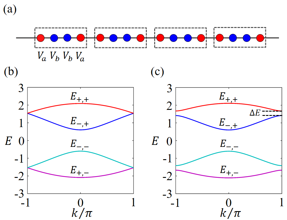
Figure 1: (a) Illustration of a 1D lattice with inversion-symmetric onsite potentials $V_{a}$ and $V_{b}$. Each unit cell consists of four sublattice sites indexed by 1 to 4 (from left to right). (b) and (c) Energy spectra for 1D superconductor with onsite potentials $V_{a}=-V_{b}=0$ and $V_{a}=-V_{b}=0.2$, respectively. The superconductor order parameter is set to be $\Delta_{0}=0.6$ in (b) and (c). Common parameter is set to be $t=1$.

We first consider a simple model, i.e., 1D $s$-wave superconductor, to present topologically protected Bogoliubov edge excitations emerging in the presence of inversion-symmetric potentials, as shown in Fig. 1(a). Its physics is described by the Hamiltonian $\hat{H}=\hat{H}_{0}+\hat{H}_{V}$. The first part reads

$$\hat{H}_{0}=t\sum_{\left\langle i,j\right\rangle,\sigma}\hat{c}_{i,\sigma}^{\dagger}\hat{c}_{j,\sigma}+\sum_{i}\left(\Delta_{0}\hat{c}_{i,\uparrow}^{\dagger}\hat{c}_{i,\downarrow}^{\dagger}+h.c.\right),$$ (1)

where $t$ denotes the tunneling strength between nearest neighbor sites, $\left\langle...\right\rangle$ represents the summation over all nearest-neighbor sites, $\sigma=\left(\uparrow,\downarrow\right)$ is the spin index, and $\Delta_{0}$ is an $s$-wave superconductor order parameter. The second term $\hat{H}_{V}=\sum_{i}V_{i}\hat{c}_{i,\sigma}^{\dagger}\hat{c}_{i,\sigma}$ describes onsite potentials with inversion symmetry. In the following, we consider each unit cell consisting of four sublattices with the potentials $V_{i}=V_{a}$ if $\mathop{\mathrm{m}od}\left(i,4\right)=0$ or $1$ and $V_{i}=V_{b}$ if $\mathop{\mathrm{m}od}\left(i,4\right)=2$ or $3$. For simplicity, we set $V_{a}=-V_{b}=V$ throughout the paper if not otherwise specified. We set nearest-neighbor hopping as the unit of energy.

Through the Fourier transformation, the Hamiltonian $\hat{H}$ for the system with periodic boundary conditions can be written as $\hat{H}=\sum_{\mathbf{k}}\hat{C}_{\mathbf{k}}^{{\dagger}}H\left(\mathbf{k}\right)\hat{C}_{\mathbf{k}}$ with

$$H\left(k\right) = ts_{x}s_{0}\sigma_{0}\tau_{z}+\xi_{+}s_{x}s_{x}\sigma_{0}\tau_{z}+\xi_{-}s_{y}s_{y}\sigma_{0}\tau_{z}$$ (2)

$$+\xi_{0}\left(s_{x}s_{y}\sigma_{0}\tau_{z}+s_{y}s_{x}\sigma_{0}\tau_{z}\right)-\Delta_{0}s_{0}s_{0}\sigma_{y}\tau_{y}$$

$$+Vs_{z}s_{z}\sigma_{0}\tau_{z}$$

under the basis $\hat{C}_{\mathbf{k}}^{\dagger}=\left(\hat{\psi}_{\mathbf{k}\uparrow}^{{\dagger}},\hat{\psi}_{\mathbf{k}\downarrow}^{\dagger},\hat{\psi}_{-\mathbf{k}\uparrow},\hat{\psi}_{-\mathbf{k}\downarrow}\right)$, where $\hat{\psi}_{\mathbf{k}\sigma}^{{\dagger}}=$ $\left(\hat{c}_{1,\mathbf{k},\sigma}^{\dagger},\hat{c}_{2,\mathbf{k},\sigma}^{\dagger},\hat{c}_{3,\mathbf{k},\sigma}^{\dagger},\hat{c}_{4,\mathbf{k},\sigma}^{\dagger}\right)$, $\hat{\psi}_{-\mathbf{k}\sigma}=$ $\left(\hat{c}_{1,-\mathbf{k},\sigma},\hat{c}_{2,-\mathbf{k},\sigma},\hat{c}_{3,-\mathbf{k},\sigma},\hat{c}_{4,-\mathbf{k},\sigma}\right)$, the quantity $\xi_{\pm}=\frac{t}{2}\left(1\pm\cos k\right)$, and $\xi_{0}=\frac{t}{2}\sin k$. The Pauli matrices $\bm{s}$, $\bm{\sigma}$, $\bm{\tau}$ act on sublattice space, spin space and particle-hole space, respectively, while the nought subscripts represent identity matrices.

The system preserves time-reversal ($\mathcal{T}$), particle-hole ($\mathcal{P}$) and chiral symmetries ($\mathcal{C}$). The energy spectra for the system are given by

$$E_{\pm,+} = \pm\sqrt{\Delta_{0}^{2}+2t^{2}+V^{2}+2t\sqrt{t^{2}\cos^{2}\frac{k}{2}+V^{2}}},$$ (3)

$$E_{\pm,-} = \pm\sqrt{\Delta_{0}^{2}+2t^{2}+V^{2}-2t\sqrt{t^{2}\cos^{2}\frac{k}{2}+V^{2}}}.$$ (4)

Each energy level is four-fold degenerate. The energy gap for the two excitation bands $E_{+,+}$ and $E_{-,+}$ at high-symmetry momentum point $k=\pi$ is $\Delta E=\sqrt{\Delta_{0}^{2}+t^{2}+\left(t+V\right)^{2}}-\sqrt{\Delta_{0}^{2}+t^{2}+\left(t-V\right)^{2}}$. In the absence of inversion-symmetric potentials, namely $V=0$, the two Bogoliubov excitation bands are degenerate at $k=\pi$ with $\Delta E=0$, as illustrated in Fig. 1(b). When $V\neq 0$, an energy gap $\Delta E\neq 0$ is opened, as shown in Fig. 1(c). Therefore, the introduction of inversion-symmetric potentials opens the gap for excitation bands, which implies a topological phase transition as discussed in the following.

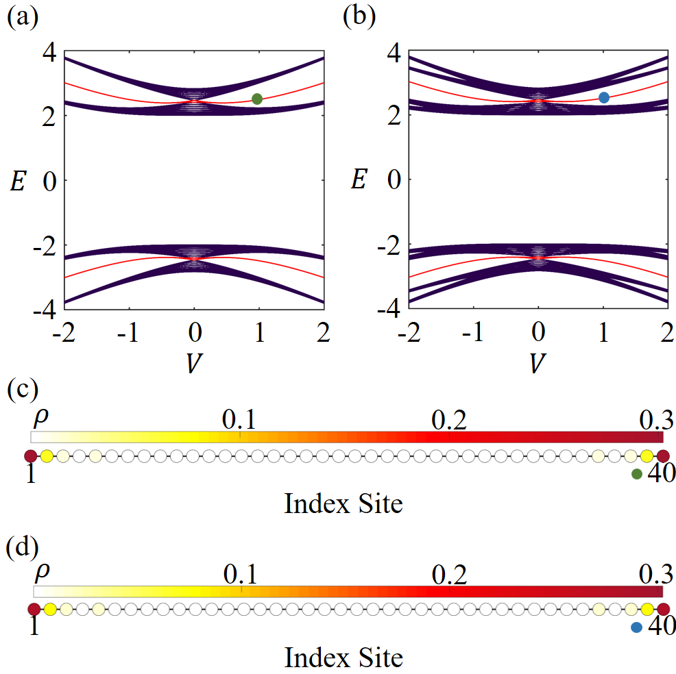
Figure 2: (a) and (b) Eigenspectrum versus inversion-symmetric onsite potential $V$ for a 1D lattice with $40$ sites. The in-gap red lines denote four-degenerate Bogoliubov edge excitation modes, where each edge of 1D lattice hosts two localized modes. In panel (a), we set $V_{a}=-V_{b}=V$ while in (b), we choose $V_{a}=V$, $V_{b}=-0.8V$. (c) and (d) The particle density distribution versus the site index, corresponding to the colored dish in panels (a) and (b) respectively. To be specific, in panel (c) $V_{a}=-V_{b}=V=1$ and in panel (d) $V_{a}=1,$ $V_{b}=-0.8$. Common parameters are set to be $\Delta_{0}=2$, $t=1$.

To demonstrate the topological properties of the system, the eigenenergies for a chain with open boundaries are computed and plotted in Fig. 2(a). We observe four degenerate states emerge at the gap between the excitation bands. Two states localize at the left end and the other two localize at the right end of the chain, as illustrated in Fig. 2(c). So far, we have focused on the special cases $V_{a}=-V_{b}=V$ for simplicity. We would like to remark that if $V_{a}\neq-V_{b}$, the system also preserve the inversion symmetry, and the Bogoliubov edge states could also be driven from a the conventional $s$-wave superconductor. In Fig. 2(b) and (d), we showcase the band structure and corresponding edge states with $V_{a}\neq-V_{b}$. It demonstrates that topological edge states also emerge on the 1D lattice. Therefore, the inversion symmetry is the crucial condition to induce the Bogoliubov edge states in the $s$-wave superconductor.

We would use the Wilson loop approach to characterize the bulk topology of the system with inversion symmetry. The base momentum point is set to be $k$. The corresponding Bloch wave functions are denoted by $\left|u_{m}\left(k\right)\right\rangle$ with $m$ representing the band index. We construct a matrix $M\left(k\right)=\left(\left|u_{m}\left(k\right)\right\rangle,\left|u_{m+1}\left(k\right)\right\rangle,...,\left|u_{n}\left(k\right)\right\rangle\right)$, where $n$ stands for the number for occupied bands. The Wilson loop operator then is defined as

$$\mathcal{W} = M\left(k\right)M\left(k+\Delta k\right)\cdots M\left(k+\left(N-1\right)\Delta k\right)$$ (5)

$$M\left(k+N\Delta k\right),$$

where $\Delta k=2\pi/N$, and $N$ is the number of unit cells. The effective Hamiltonian is defined by $\mathcal{H}=-i\ln\mathcal{W}/\pi$. The eigenvalues for $\mathcal{H}$ are denoted by $v_{s}$ with $s=1,2,...,n$. The bulk topological invariant is then given by $\xi=\sum_{s=1}^{n}v_{s}$. Through numerical calculations, the topological invariant is given by $\xi=\pm 2$ in superconductor phase if $V\neq 0$, suggesting two localized Bogoliubov edge excitations would appear at each one edge of the 1D lattice, as demonstrated in Fig. 2. The localized Bogoliubov edge excitations are topologically protected and robust against inversion-symmetric perturbations as long as the bulk energy gap remains open.

The above simple toy model exhibits interesting topological properties induced by inversion-symmetric potentials. However, the long-range superconductor order is forbidden due to the strong quantum fluctuations. In the following, we would propose a realistic platform to manifest intrinsic first-order and higher-order topology, whose topology can be explicitly understood from the above 1D model.

III Bogoliubov corner excitations in an $S$-wave superfluid on a square lattice

Here we consider ultracod Fermionic atoms with pseudo spin loaded in a 2D square lattice. The physics for the system is described by a tight-binding Hamiltonian as

$$\hat{H}_{\mathrm{squ},0}=-t\sum_{\left\langle i,j\right\rangle}\hat{c}_{i,\sigma}^{\dagger}\hat{c}_{j,\sigma}-U\sum_{i}\hat{n}_{i,\uparrow}\hat{n}_{i,\downarrow}-\mu\sum_{i,\sigma}\hat{n}_{i,\sigma},$$ (6)

where $U$ is the strength of an onsite attractive $\mathrm{SU(2)}$-invariant interaction, and $\mu$ denotes the chemical potential. Given a local dip potential with mirror symmetry applied to a one-dimensional line as shown in Fig. 3(a), the one-dimensional defect chain also enjoys the mirror symmetry along $x$. The total Hamiltonian then becomes

$$\hat{H}_{\mathrm{squ}}=\hat{H}_{\mathrm{squ},0}+\sum_{i\in\mathrm{Def},\sigma}V_{i}\hat{n}_{i,\sigma},$$ (7)

where $V_{i}=V_{a}=V$ for $\mathop{\mathrm{m}od}\left(i_{x},4\right)=1,0$ and $V_{i}=V_{b}=-V$ for $\mathop{\mathrm{m}od}\left(i_{x},4\right)=2,3$ on sites on the defect chain “$\mathrm{Def}$”.

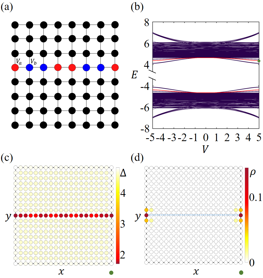
Figure 3: (a) Illustration of a square lattice with a defect chain respecting the mirror symmetry. (b) Eigenspectrum for the $s$-wave superfluid versus mirror-symmetric onsite potential $V$ on the 20$\times$19 square lattice. The in-gap red lines indicate four-degenerate Bogoliubov corner excitation modes. (c) Distributions of $s$-wave superfluid order parameters on the square lattice with a defect chain. (d) Particle density distributions of the in-gap states. The blue dashed line denotes the defect chain. The Bogoliubov excited states shown in (c) and (d) have been indicated by the green dot in (b) with the mirror-symmetric onsite potential $V=5$. Common parameters in (b)-(d) are set to be $t=1$, $U=10$, $\mu=0.05$.

As the interaction $U$ becomes stronger, the fermions would be paired and enter a superfluid phase when $U$ exceeds a critical value. The superfluid order at the lattice site $i$ is assumed as $\Delta_{i}=U\left\langle\hat{c}_{i,\uparrow}^{\dagger}\hat{c}_{i,\downarrow}^{\dagger}\right\rangle$, and the interaction term becomes $-U\sum_{i}\hat{n}_{i,\uparrow}\hat{n}_{i,\downarrow}=\sum_{i}\left(-\Delta_{i}^{\ast}\hat{c}_{i,\uparrow}^{\dagger}\hat{c}_{i,\downarrow}^{\dagger}-\Delta_{i}\hat{c}_{i,\downarrow}\hat{c}_{i,\uparrow}+\left|\Delta_{i}\right|^{2}/U\right)$ at the mean-field level. Through the Bogoliubov-Valatin transformation, the creation operators $\hat{c}_{i,\uparrow}^{\dagger}$ and $\hat{c}_{i,\downarrow}^{\dagger}$ are written as $\hat{c}_{i,\uparrow}^{\dagger}=\sum_{n=1}^{2N_{u}}\left(u_{i,\uparrow}^{n\ast}\hat{\psi}_{n}^{\dagger}-\upsilon_{i,\uparrow}^{n}\hat{\psi}_{n}\right)$ and $\hat{c}_{i,\downarrow}^{\dagger}=\sum_{n=1}^{2N_{u}}\left(u_{i,\downarrow}^{n\ast}\hat{\psi}_{n}^{\dagger}+\upsilon_{i,\downarrow}^{n}\hat{\psi}_{n}\right)$, where $N_{u}$ is the number of unit-cells, and $\hat{\psi}_{n}^{\dagger}$ and $\hat{\psi}_{n}$ are creation and annihilation operators for Bogoliubov quasi-particles such that the Hamiltonian $\hat{H}_{\mathrm{squ}}$ can be diagonalized. The coefficients $u_{i,\sigma}^{n}$ and $\upsilon_{i,\sigma}^{n}$ can be derived from the following equations

$$\sum_{j}\hat{H}_{\mathrm{0},ij,\sigma}u_{j,\sigma}^{n}-\Delta_{i}\upsilon_{i,\bar{\sigma}}^{n} = E_{n}u_{i,\sigma}^{n},$$ (8)

$$-\sum_{j}\hat{H}_{\mathrm{0},ji,\sigma}\upsilon_{j,\sigma}^{n}-\Delta_{i}^{\ast}u_{i,\bar{\sigma}}^{n} = E_{n}\upsilon_{i,\sigma}^{n},$$ (9)

where $\hat{H}_{\mathrm{0},ij,\sigma}$ denotes the element of the Hamiltonian matrix $\hat{H}_{\mathrm{squ}}$ with $U=0$ under the basis $\hat{\Psi}=\left(\hat{C}_{1},...,\hat{C}_{m},...,\hat{C}_{2N_{u}}\right)^{T}$ with $\hat{C}_{m}=\left(\hat{c}_{m,\uparrow},\hat{c}_{m,\downarrow}\right)$.

Through the numeric calculations, we compute the superfluid order parameter at each lattice site on a square optical lattice under open boundary conditions, as shown in Fig. 3(c). The superfluid order on the defect chain is weaker than that in other regions due to the non-zero mirror symmetric potentials. In addition, we observe that the superfluid order on the boundary is stronger than that in the bulk, and the superfluid order in the bulk is nearly uniform. This is consistent to the intuition that the lattice sites in the bulk are less affected by the boundary. The eigen-energy distributions versus potential $V$ have been shown in Fig. 3(b), indicating isolated states (denoted by red lines) emerge in the energy gap for Bogoliubov quasiparticles. The particle density distributions for the isolated states, as plotted in Fig. 3(d), showcase these in-gap states are localized at the end of the defect chain.

We would like to remark that the above defect chain can be considered as a one-dimensional $s$-wave superfluid imprinted on the 2D lattice. While the defect chain couples with other chains, it also exhibits topological nontrivial properties as long as the energy gap remains open.

IV Bogoliubov corner excitations in an $S$-wave superfluid on a honeycomb lattice

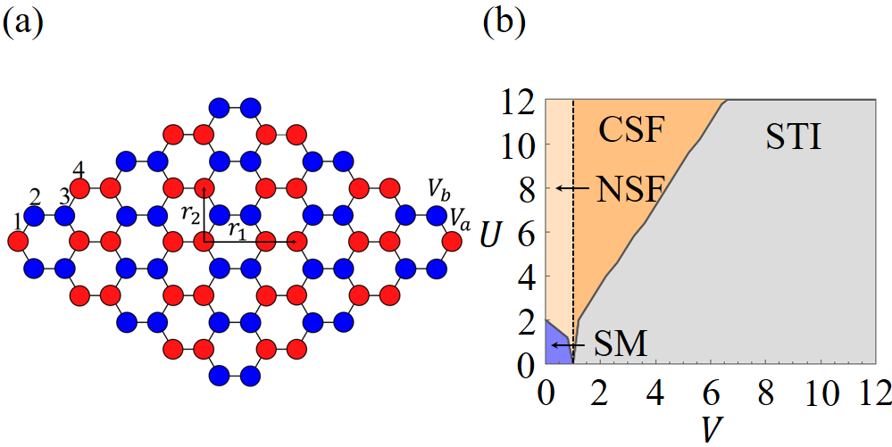
Figure 4: (a) Illustration of a honeycomb lattice with a mirror-symmetric onsite potential. Each unit-cell consists of four sublattice sites indexed by 1 to 4. (b) A rich global phase diagram plotted against the potential and interaction strength including second-order topological insulators (STI), semimetal (SM), normal superfluid (NSF) and superfluid with Bogoliubov corner excitations (CSF) .

Consider a two-component Fermi gas loaded in a 2D honeycomb optical lattice with a uniform chemical potential. Turning on the onsite attractive interaction for fermionic atoms, the fermions would be paired and enter the $s$-wave superfluid phase from the semimetal phase when the interaction exceeds a critical value Zhao2006 . Its Bogliubov excitations are gapless and show trivial properties. Hereafter, we would consider there exists onsite potential with mirror symmetry as shown in Fig. 4(a), and showcase Bogoliubov corner excitations could be induced from the excitation bands.

At the mean-field level, the physics of a system with a mirror-symmetric potential is described by the Hamiltonian as

$$h_{h} = \lambda_{0}(s_{y}s_{x}\sigma_{0}\tau_{z}+s_{x}s_{y}\sigma_{0}\tau_{z})+A_{k}+\lambda_{a}s_{x}s_{x}\sigma_{0}\tau_{z}$$ (10)

$$+\lambda_{b}s_{x}s_{0}\sigma_{0}\tau_{z}+\lambda_{c}s_{y}s_{0}\sigma_{0}\tau_{z}+\lambda_{k}s_{y}s_{y}\sigma_{0}\tau_{z}$$

under the basis vector $\hat{C}_{\mathbf{k}}^{\dagger}=\left(\hat{\psi}_{\mathbf{k}\uparrow}^{{\dagger}},\hat{\psi}_{\mathbf{k}\downarrow}^{\dagger},\hat{\psi}_{-\mathbf{k}\uparrow},\hat{\psi}_{-\mathbf{k}\downarrow}\right)$ with $\hat{\psi}_{\mathbf{k}\sigma}^{{\dagger}}=$ $\left(\hat{c}_{1,\mathbf{k},\sigma}^{\dagger},\hat{c}_{2,\mathbf{k},\sigma}^{\dagger},\hat{c}_{3,\mathbf{k},\sigma}^{\dagger},\hat{c}_{4,\mathbf{k},\sigma}^{\dagger}\right)$ and $\hat{\psi}_{-\mathbf{k}\sigma}=$ $\left(\hat{c}_{1,-\mathbf{k},\sigma},\hat{c}_{2,-\mathbf{k},\sigma},\hat{c}_{3,-\mathbf{k},\sigma},\hat{c}_{4,-\mathbf{k},\sigma}\right)$, where $\lambda_{0}=t\sin k_{\alpha}$, $\lambda_{a}=\frac{1}{2}t(1+\cos k_{\alpha})$, $\lambda_{b}=t(1+\cos\sqrt{3}k_{y})$, $\lambda_{c}=t\sin\sqrt{3}k_{x}$, $\lambda_{k}=\frac{1}{2}t(1-\cos k_{\alpha})$, $k_{\alpha}=\mathbf{k}\cdot\left(\mathbf{r}_{1}+\mathbf{r}_{2}\right)=3k_{x}+\sqrt{3}k_{y}$, $A_{k}=\Delta_{1}s_{+}s_{+}\sigma_{y}\tau_{z}+\Delta_{2}s_{-}s_{+}\sigma_{y}\tau_{z}+\Delta_{3}s_{+}s_{-}\sigma_{y}\tau_{z}+\Delta_{4}s_{-}s_{-}\sigma_{y}\tau_{z}+V_{+}s_{0}s_{0}\sigma_{0}\tau_{z}+V_{-}s_{z}s_{z}\sigma_{0}\tau_{z}$ with $V_{\pm}=\left(V_{a}\pm V_{b}\right)/2$ and $s_{\pm}=\left(s_{0}\pm s_{z}\right)/2$. $\Delta_{m=1,2,3,4}$ denotes the superfluid order parameter on the sublattice site $m$ as indexed in Fig. 4(a). The self-consistent equations for the superfluid order and particle filling ratio are given by

$$\Delta_{m} = \frac{U}{N_{u}}\sum_{k\in BZ/2}\left\langle\hat{c}_{m,-\mathbf{k},\downarrow}\hat{c}_{m,\mathbf{k},\uparrow}\right\rangle,$$ (11)

$$n_{m} = \frac{1}{N_{u}}\sum_{k\in BZ/2}\left\langle\hat{c}_{m,\mathbf{k},\uparrow}^{\dagger}\hat{c}_{m,\mathbf{k},\uparrow}+\hat{c}_{m,\mathbf{k},\downarrow}^{\dagger}\hat{c}_{m,\mathbf{k},\downarrow}\right\rangle.$$ (12)

Through numerical self-consistent calculations for Eqs. (11) and (12), we find $\Delta_{m}\equiv\Delta$ and $n_{m}\equiv n$ for all $m$ at zero temperature. The rich phase diagram, which has been shown in Fig. 4(b), exhibits a range of interesting and physically distinctive phases including semimetal (SM), second-order topological insulator (STI), and superfluid phases with a non-zero superfluid order (normal superfluid and superfluid with Bogoliubov corner excitations). Fig. 4(b) showcases that at fixed interaction, for example $U=4$, as $V$ becomes larger, the system would enter STI since it’s hard to form pairing when $V$ exceeds a critical value.

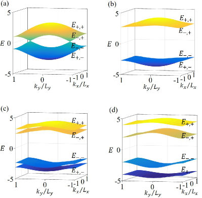
Figure 5: Energy spectra for different onsite potentials $V$. In (a), $U=V=0$. In (b), $U=6$, $V=0$. In (c), $U=6$, $V=1$. In (d), $U=6$, $V=3$. Common parameters are set to be $t=1$, $L_{x}=\pi/3$, $L_{y}=\pi/\sqrt{3}$.

We compute the energy spectra for the superfluid under periodic boundary conditions and the numerical results are presented in Fig. 5. We observe the $s$-wave superfluid order opens the energy gap for the Dirac semimetal, as shown in Figs. 5(a) and (b). However, the Bogoliubov excitation band remains gapless. After turning on the onsite potential with mirror symmetry, an direct energy gap emerges, as depicted in Fig. 5(c). As the potential strength increases, the energy gap becomes larger and a full gap exists when the potential exceeds a critical value, as illustrated in Fig. 5(d).

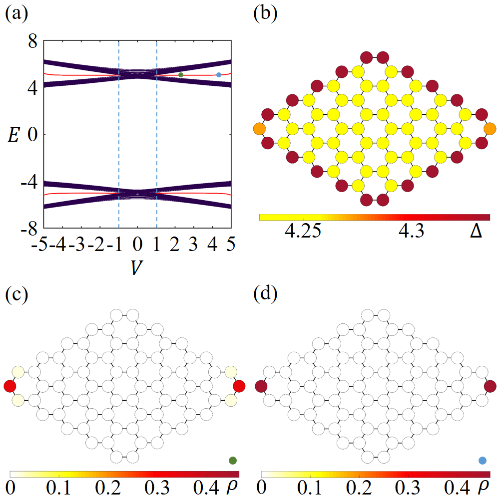
Figure 6: (a) Eigenspectrum versus mirror-symmetric onsite potential $V$ for the honeycomb lattice. The in-gap red lines denote four-degenerate Bogoliubov corner excitation modes. (b) Distributions of $s$-wave superfluid order parameters on the honeycomb lattice. (c) and (d) Particle density distributions of the in-gap states. These chosen parameters in sub-figures also have been indicated by colored dots in (a). In (b) and (c), $V_{a}=-V_{b}=V=2.2$. In (d), $V_{a}=-V_{b}=V=4.5$. Common parameters are set to be $t=1$, $U=10$.

To explore the nontrivial properties of Bogoliubov excitation bands, we calculate the eigenenergies for the superfluid versus $V$ with fixed interaction $U$ under open boundary conditions. Four degenerate states emerge in the energy gap for Bogolibov excitations, as shown by the red lines with four-fold degenerates in Fig. 6(a). They are localized at two corners of the sample as shown in Fig. 6(c). Through the numeric calculations, we compute the superfluid order parameters at each lattice site on a honeycomb optical lattice under open boundary conditions, as shown in Fig. 6(b), we can observe that the bulk superfluid order is uniform. Through comparing Fig. 6 (c) with (d), it’s also clear that with increasing potential $V$, the Bogoliubov corner modes become more localized. In summary, there are superfluid phases with two different Bogoliubov excitations, one with gapless Bogliubov excitation bands dubbed NSF, and the other with gapped Bogliubov excitation bands called CSF. Both phases and the their phase transition are demonstrated in the phase diagram in Fig. 4(b).

The Bogoliubov corner excitations is the exhibition of the bulk topology, characterized by the topological invariant protected by mirror symmetry. Taking a similar procedure as in the one-dimensional case above, the topological invariant at each $k_{y}$ is defined by

$$\xi_{x}\left(k_{y}\right)=-\frac{i}{\pi}\mathrm{Tr}\left(\ln\mathcal{W}_{x,k}\right),$$ (13)

where the Wilson loop operator reads $\mathcal{W}_{x,k}=F_{x,k+N_{x}\Delta k_{x}}...F_{x,k+\Delta k_{x}}F_{x,k}$, $\Delta k_{x}=2\pi/N_{x}$, and $N_{x}$ is the number of unit cells in the $x$ direction. The entry of matrix $F_{x,k}$ is $\left[F_{x,k}\right]^{m,n}=\left\langle u_{m,k+\Delta k_{x}}|u_{m,k}\right\rangle$ with $\left|u_{m,k}\right\rangle$ being the Bloch wave function of the energy bands $E_{m}\left(k\right)$, i.e., $h_{h}\left(k\right)u_{m,k}=E_{m}\left(k\right)$ while $\xi_{x}\left(k_{y}\right)$ forms the Wannier bands. Finally, the topological invariant is defined as $(\xi_{x}^{\prime},\xi_{y}^{\prime})$, where $\xi_{x}^{\prime}=\frac{1}{2N_{y}}\sum_{k_{y}}\xi_{x}\left(k_{y}\right)$, and $\xi_{y}^{\prime}$ takes similar form as $\xi_{x}^{\prime}$. Through numeric calculations, we obtain the topological invariant $(\xi_{x}^{\prime},\xi_{y}^{\prime})=(2,0)$ in the CSF regime and $(0,0)$ in NSF regime, as shown in Fig. 4(b). In summary, the $s$-wave superfluid phase have two different types of Bogoliubov excitations: trivial Bologliubov excitations in NSF regime, and higher-order Bogoliubov corner excitations in CSF regime. We emphasize that the ground state of the $s$-wave superfluid in both regimes is topologically trivial. The topological property of excited corner modes originates from the Bogoliubov excitation bands.

V Discussions and Conclusions

The $s$-wave superfluid with a uniform chemical potential exhibits trivial Bogoliubov excitation on a 1D lattice, and 2D square or honeycomb lattice. Intriguingly, we find the onsite potential with mirror symmetry could open the energy gap in Bogoliubov excitation spectrums. The Bogliubov excitation bands exhibit topological nontrivial properties and the edge modes manifest themselves as zero-dimensional (0D) Bogliubov excitations localized at the end of a 1D lattice and the corners of a 2D honeycomb lattice, although the ground states for the systems remains in a trivial phase. Since the systems preserve inversion or mirror symmetry, the winding number can characterize the nontrivial excitation band.

We would like to remark that our model in this work can be implemented in ultracold atoms. For instance, the mirror-symmetric potential on 2D square lattice can be achieved through a pair of coherent counterpropagating laser beams with wave length $2a$ and $8a$ along $x$. The onsite attractive interaction could be finely tuned through Feshbach Resonance technique.

In summary, we propose that topological Bogoliubov excitations can be induced solely by onsite potentials in a topologically trivial conventional $s$-wave superfluid. The edge excitations manifest themselves as 0D modes localized at edges or corners of the system. These modes are robust against inversion or mirror symmetric perturbations as it preserves the degeneracy. Our work provides new insights for understanding higher-order topological states in conventional superconductors and superfluids, and also provides realistic platforms for engineering nontrivial Bogoliubov corner excitations in real experiments.

- (1) W. A. Benalcazar, B. A. Bernevig, and T. L. Hughes, Quantized electric multipole insulators, Science 357, 61 (2017).
- (2) J. Langbehn, Y. Peng, L. Trifunovic, F. von Oppen, and P. W. Brouwer, Refection-Symmetric Second-Order Topological In sulators and Superconductors, Phys. Rev. Lett. 119, 246401 (2017).
- (3) Z. Song, Z. Fang, and C. Fang, ()-Dimensional EdgeStates of Rotation Symmetry Protected Topological States, .Phys. Rev. Lett. 119, 246402 (2017)
- (4) A.P. Schnyder, S. Ryu, A. Furusaki, A.W.W. Ludwig, Classification of topological insulators and superconductors in three spatial dimensions, Phys. Rev. B 78, 195125 (2008).
- (5) A. Kitaev, Periodic table for topological insulators and superconductors, AIP Conference Proceedings, 1134, 22 (2009).
- (6) S. Ryu, A.P. Schnyder, A. Furusaki, A.W.W. Ludwig, Topological insulators and superconductors: ten-fold way and dimensionality hierarchy, New J. Phys. 12, 065010 (2010).
- (7) E. Khalaf, Higher-order topological insulators and superconductors protected by inversion symmetry, Phys. Rev. B 97, 205136 (2018).
- (8) G. van Miert and C. Ortix, Higher-order topological in sulators protected by inversion and rotoinversion symmetries, Phys. Rev. B 98, 081110(R) (2018).
- (9) E. Cornfeld and A. Chapman, Classification of crystalline topological insulators and superconductors with point group symmetries, Phys. Rev. B 99, 075105 (2019).
- (10) M. Geier, P. W. Brouwer and L. Trifunovic, Symmetry-based indicators for topological Bogoliubov–de Gennes Hamiltonians, Phys. Rev. B 101, 245128 (2020).
- (11) E. Cornfeld and S. Carmeli, Tenfold topology of crys tals: Unified classification of crystalline topological in sulators and superconductors, Phys. Rev. Research 3, 013052 (2021).
- (12) Z. Yan, F. Song, and Z. Wang, Majorana corner modes in a high-temperature platform, Phys. Rev. Lett. 121, 096803 (2018).
- (13) Q. Wang, C.-C. Liu, Y.-M. Lu, and F. Zhang, High temperature Majorana corner states, Phys. Rev. Lett. 121, 186801 (2018).
- (14) C.-H. Hsu, P. Stano, J. Klinovaja, and D. Loss, Majorana Kramers Pairs in Higher-Order Topological Insulators, Phys. Rev. Lett. 121, 196801 (2018).
- (15) T. Liu, J. J. He, and F. Nori, Majorana corner states in a two-dimensional magnetic topological insulator on a high-temperature superconductor, Phys. Rev. B 98, 245413 (2018).
- (16) X.-H. Pan, K.-J. Yang, L. Chen, G. Xu, C.-X. Liu, and X. Liu, Lattice symmetry assisted second order topological superconductors and Majorana patterns, Phys. Rev. Lett. 123, 156801 (2019).
- (17) X. Zhu, Second-Order Topological Superconductors with Mixed Pairing, Phys. Rev. Lett. 122, 236401 (2019).
- (18) Y. Peng and Y. Xu, Proximity-induced Majorana hinge modes in antiferromagnetic topological insulators, Phys. Rev. B 99, 195431 (2019).
- (19) Y.-J. Wu, J. Hou, Y.-M. Li, X.-W. Luo, X. Shi, and C. Zhang, In-plane Zeeman field induced Majorana corner and hinge modes in an s-wave superconductor heterostructure, Phys. Rev. Lett. 124, 227001 (2020).
- (20) K. Laubscher, D. Chughtai, D. Loss, and J. Klinovaja, Kramers pairs of Majorana corner states in a topological insulator bilayer, Phys. Rev. B 102, 195401 (2020).
- (21) R.-X. Zhang, W.S. Cole, and S. Das Sarma, Helical hinge majorana modes in iron-based superconductors, Phys. Rev. Lett. 122, 187001 (2019).
- (22) R.-X. Zhang, W. S. Cole, X. Wu, and S. Das Sarma, Higher-Order Topology and Nodal Topological Superconductivity in Fe(Se,Te) Heterostructures, Phys. Rev. Lett. 123, 167001 (2019).
- (23) M. J. Gray, J. Freudenstein, S. Yang, F. Zhao, R. O’Connor, S. Jenkins, N. Kumar, M. Hoek, A. Kopec, S. Huh, T. Taniguchi, K. Watanabe, R. Zhong, C. Kim, G. D. Gu and K. S. Burch, Evidence for Helical Hinge Zero Modes in an Fe-Based Superconductor, Nano Lett. 19, 4890 (2019).
- (24) X. Wu, W. A. Benalcazar, Y. Li, R. Thomale, C.-X. Liu, and J. Hu, Boundary-Obstructed Topological High- Superconductivity in Iron Pnictides, Phys. Rev. X 10, 041014 (2020).
- (25) M. Kheirkhah, Z. Yan, and F. Marsiglio, Vortex-line topology in iron-based superconductors with and without second-order topology, Phys. Rev. B 103, L140502 (2021).
- (26) S. Qin, C. Fang, F.-C. Zhang, and J. Hu, Topological Superconductivity in an Extended -Wave Superconductor and Its Implication to Iron-Based Superconductors, Phys. Rev. X 12, 011030 (2022).
- (27) Y. Volpez, D. Loss, and J. Klinovaja, Second order topological superconductivity in -junction Rashba layers, Phys. Rev. Lett. 122, 126402 (2019).
- (28) S.-B. Zhang and B. Trauzettel, Detection of second-order topological superconductors by Josephson junctions, Phys. Rev. Research 2, 012018(R) (2020).
- (29) C. Zeng, T. D. Stanescu, C. Zhang, V. W. Scarola, and S. Tewari, Majorana corner modes with solitons in an attractive Hubbard-Hofstadter model of cold atom optical lattices, Phys. Rev. Lett. 123, 060402 (2019).
- (30) B. Huang, G. Luo, and N. Xu, Mirror-symmetry-protected topological superfluid and second-order topological superfluid in bilayer fermionic gases with spin-orbit coupling, Phys. Rev. A 100, 023602 (2019).
- (31) Z. Wu, Z. Yan, and W. Huang, Higher-order topological superconductivity: Possible realization in Fermi gases and Sr2RuO4, Phys. Rev. B 99, 020508(R) (2019).
- (32) M. Kheirkhah, Z. B. Yan, Y. Nagai, and F. Marsiglio, First- and Second-Order Topological Superconductivity and Temperature-Driven Topological Phase Transitions in the Extended Hubbard Model with Spin-Orbit Coupling, Phys. Rev. Lett. 125, 017001 (2020).
- (33) Y.-B. Wu, G.-C. Guo, Z. Zheng, and X.-B. Zou, Effective Hamiltonian with tunable mixed pairing in driven optical lattices, Phys. Rev. A 101, 013622 (2020).
- (34) Y. J. Wu, T.-B. Gao, N. Li, J. Zhou and S.-P. Kou, Majorana corner modes in an -wave second order topological superfluid, J. Phys.: Condens. Matter 32, 145601 (2020).
- (35) Y.-B. Wu, G.-C. Guo, Z. Zheng, and X.-B. Zou, Multiorder topological superfluid phase transitions in a two-dimensional optical superlattice, Phys. Rev. A 104, 013306 (2021).
- (36) Y.-B Wu, Z. Zheng, X.-G Qiu, L. Zhuang, G.-C Guo, X.-B Zou, and W.-M Liu, Tunable boson-assisted finite-range interaction and engineering Majorana corner modes in optical lattices, Phys. Rev. A 107, 043304 (2023).
- (37) K. Laubscher, D. Loss, and J. Klinovaja, Majorana and parafermion corner states from two coupled sheets of bilayer graphene, Phys. Rev. Research 2, 013330 (2020).
- (38) A. Chew, Y.-J Wang, B. A. Bernevig, and Z.-D Song, Higher-order topological superconductivity in twisted bilayer graphene, Phys. Rev. B 107, 094512 (2023).
- (39) E. Zhao and A. Paramekanti, BCS-BEC Crossover on the Two-Dimensional Honeycomb Lattice, Phys. Rev. Lett. 97, 230404 (2006).