Correlation of dynamical density fluctuation in presence of an external magnetic field and its implication on QCD critical point

Abstract

The dynamical correlation of density fluctuation in quark gluon plasma has been investigated within the scope of the Müller-Israel-Stewart theory in the presence of a high external magnetic field. The dynamic structure factor of the density fluctuation exhibits three Lorentzian peaks in the absence of an external magnetic field- a central Rayleigh peak and two Brillouin peaks situated symmetrically on the opposite sides of the Rayleigh peak. The spectral structure displays five peaks in the presence of a magnetic field due to the coupling of the magnetic field with the thermodynamic fields in second-order hydrodynamics. The emergence of the extra peaks originates due to the asymmetry in the pressure gradient caused by the external magnetic field in the system. As a consequence, enhancement in the elliptic flow is expected in a nearly central collision. It is also found that near the critical point, all the Brillouin peaks disappear irrespective of the presence or absence of the external magnetic field.

I Introduction

One of the primary objectives of heavy-ion collision (HIC) experiments at Relativistic Heavy Ion Collider (RHIC) and the Large Hadron Collider (LHC) is to create and characterize a deconfined state of thermal quarks and gluons, called quark gluon plasma (QGP). It is expected that after a proper time $\tau_{0}\sim 1fm/c$ of the collision, the system enters a state of local thermal equilibrium. The evolution of the QGP in spacetime can be studied by using relativistic hydrodynamics Chaudhuri (2014); Heinz and Snellings (2013); Gale et al. (2013); Romatschke and Romatschke (2019), which is a low frequency or long wavelength effective theory of the many body interacting systems. In the non-central collisions of nuclei at RHIC and LHC energies, a large electromagnetic (EM) field is produced due to the electric current generated by the accelerated motion of charged spectators, i.e. protons. In non-central collisions of heavy nuclei (Au+Au or Pb+Pb) at RHIC and LHC energies, the transient magnetic field ($B$) can be as high as  $\sim 10^{17}\mbox{-}10^{18}$ Gauss) Bzdak and Skokov (2012); Deng and Huang (2012); Tuchin (2013); Roy and Pu (2015); Li et al. (2016). Therefore, in such a situation, it is imperative to consider the effect of $B$ on the characterization of the QGP. The survival time of $B$ crucially depends on the electrical conductivity of the QGP Gupta (2004); Aarts et al. (2015); Amato et al. (2013). The inclusion of magnetic field in relativistic hydrodynamics is studied within the ambit of relativistic magnetohydrodynamics (MHD) which is a self-consistent macroscopic framework that deals with the evolution of mutually interacting charged fluid along with the EM fields. Recently, several authors have studied the effect of the EM fields on QGP fluid in the context of special relativistic systems Huang et al. (2010); Huang (2016); Greif et al. (2017); Roy et al. (2017); Gursoy et al. (2014); Huang (2016); Inghirami et al. (2016); Huang et al. (2011).

In the relativistic viscous hydrodynamics and relativistic magnetohydrodynamics, the transport coefficients, such as the shear viscosity, bulk viscosity, thermal conductivity, etc. are taken as input which can be estimated from an underlying microscopic theory Arnold et al. (2000, 2003); Li and Yee (2018); Cao et al. (2019). A straightforward extension of the non-relativistic viscous fluid dynamics (Navier-Stokes equation) to relativistic regime (without magnetic field) Eckart (1940); Landau and Lifshitz (2013) leads to acuasal and unstable solutions Hiscock and Lindblom (1983, 1985, 1987). These issues were addressed and resolved by Müller and Israel and Stewart (MIS) Israel (1976); Israel and Stewart (1979) who developed a causal and stable second-order relativistic hydrodynamics. Here the order of the theory is dictated by different orders of gradients in the expansion hydrodynamic quantities i.e., energy-momentum tensor (EMT).

The dynamic density correlator or the structure factor, $\mathscr{S}_{nn}(\mathchoice{\mbox{\boldmath$k$}}{\mbox{\boldmath$k$}}{\mbox{\boldmath$\scriptstyle k$}}{\mbox{\boldmath$\scriptscriptstyle k$}},\omega)$, has been studied extensively in condensed matter physics by using linear response theory Stanley (1971) within the ambit of fluid dynamics. The correlation of density fluctuations can be examined through the dynamic spectral structure $\mathscr{S}_{nn}(\mathchoice{\mbox{\boldmath$k$}}{\mbox{\boldmath$k$}}{\mbox{\boldmath$\scriptstyle k$}}{\mbox{\boldmath$\scriptscriptstyle k$}},\omega)$ in wave vector ($k$), frequency ($\omega$) space. Ordinarily, for a fluid modelled by relativistic hydrodynamics, the $\mathscr{S}_{nn}(\mathchoice{\mbox{\boldmath$k$}}{\mbox{\boldmath$k$}}{\mbox{\boldmath$\scriptstyle k$}}{\mbox{\boldmath$\scriptscriptstyle k$}},\omega)$ consists of three distinct peaks, two of them are Brillouin ($B$) peaks, created due to pressure fluctuation at constant entropy and the other is the Rayleigh (R) peak, originates due to thermal or entropy fluctuation at constant pressure  Minami and Kunihiro (2010); Hasanujjaman et al. (2020).

The structure factor has been immensely investigated experimentally in condensed matter physics to determine the speed of sound by using the scattering of photons and neutrons. It is observed that the position of the B-Peaks in $\mathscr{S}_{nn}(\mathchoice{\mbox{\boldmath$k$}}{\mbox{\boldmath$k$}}{\mbox{\boldmath$\scriptstyle k$}}{\mbox{\boldmath$\scriptscriptstyle k$}},\omega)$ depends on the speed of sound and the width of both B and R peaks are determined by various transport coefficients (shear and bulk viscosities, thermal conductivity) and response functions (specific heats). For QCD (quantum chromodynamics) matter, no such external probes work which makes the direct detection of the peaks extremely difficult, if not impossible. However, such investigation may shed light on the speed of sound waves, which depends on the equation of state (EoS) of the QCD matter. In the previous studies  Minami and Kunihiro (2010); Hasanujjaman et al. (2020), the relativistic hydrodynamics is used to find out the correlation in density fluctuation in QCD matter without including magnetic field. In the present work, we have considered the relativistic MHD to study the dynamical density correlator in a baryon-rich fluid. We derive $\mathscr{S}_{nn}(\mathchoice{\mbox{\boldmath$k$}}{\mbox{\boldmath$k$}}{\mbox{\boldmath$\scriptstyle k$}}{\mbox{\boldmath$\scriptscriptstyle k$}},\omega)$, which will enable us to determine the speed of the perturbation propagating as sound waves through the QCD medium immersed in a constant magnetic field.

The manuscript is organized as follows: In Sec. II, we discuss briefly the form of energy-momentum tensor of fluid in the presence of EM fields. In the next section i.e. in Sec. III, we find the linearized hydrodynamic equation and derive the density-density correlation function. In Sec IV, we discuss important results that stems from our analysis and summary and conclusion is presented in Sec. V.

Throughout the article, we use the natural units, $c=k_{B}=\epsilon_{0}=\mu_{0}=1$ and the metric tensor is $g^{\mu\nu}=$diag$\left(+1,-1,-1,-1\right)$. The time-like fluid four velocity $u^{\mu}=\frac{1}{\sqrt{1-v^{2}}}\,(1,\mathchoice{\mbox{\boldmath$v$}}{\mbox{\boldmath$v$}}{\mbox{\boldmath$\scriptstyle v$}}{\mbox{\boldmath$\scriptscriptstyle v$}})$ satisfies the relation, $u_{\mu}u^{\mu}=1$. Also, we use the following decomposition $\partial_{\mu}\equiv u_{\mu}u_{\nu}\partial^{\nu}+(g_{\mu\nu}-u_{\mu}u_{\nu})\partial^{\nu}=u_{\mu}D+\nabla_{\mu}$. The fourth-rank projection tensor is defined as $\Delta^{\mu\nu}_{\alpha\beta}=\frac{1}{2}\left(\Delta^{\mu}_{\alpha}\Delta^{\nu}_{\beta}+\Delta^{\mu}_{\beta}\Delta^{\nu}_{\alpha}\right)-\frac{1}{3}\Delta^{\mu\nu}\Delta_{\alpha\beta}$, where $\Delta^{\mu\nu}\equiv g^{\mu\nu}-u^{\mu}u^{\nu}$ is the projection operator, such that $\Delta^{\mu\nu}u_{\nu}=0$.

II RELATIVISTIC MAGNETOHYDRODYNAMICS

In this section, first we discuss the equation of motion of electromagnetic (EM) field and magnetohydrodynamics.

II.1 Equation of motion of the EM field

We start by discussing the relativistically covariant formulation of classical electrodynamics. The second rank anti-symmetric EM field tensor $F^{\mu\nu}$, can be defined as, in terms of electric field four-vector $E^{\mu}(=F^{\mu\nu}u_{\nu})$, magnetic field four-vectors  $B^{\mu}=(\frac{1}{2}\epsilon^{\mu\nu\alpha\beta}u_{\nu}F_{\alpha\beta}=\tilde{F}^{\mu\nu}u_{\nu})$, and the fluid four-velocity $u^{\mu}$ Lichnerowicz and for Advanced Studies (1967); Anile (2005); Thorne and Blandford (2017),

$$F^{\mu\nu}=E^{\mu}u^{\nu}-E^{\nu}u^{\mu}+\epsilon^{\mu\nu\alpha\beta}u_{\alpha}B_{\beta},$$ (1)

and its dual counter part is represented by,

$$\tilde{F}^{\mu\nu}=B^{\mu}u^{\nu}-B^{\nu}u^{\mu}-\epsilon^{\mu\nu\alpha\beta}u_{\alpha}E_{\beta}.$$ (2)

where, $\epsilon^{\mu\nu\alpha\beta}$ is the Levi-Civita tensor. It is quite straight forward to see by using the anti-symmetric property of $F^{\mu\nu}$ that both $E^{\mu}$ and $B^{\mu}$ are orthogonal to $u^{\mu}$ i.e., $E^{\mu}u_{\mu}=B^{\mu}u_{\mu}=0$. It may be noted that in the rest frame $u^{\mu}=(1,\bf 0)$, $E^{\mu}=(0,\bf E)$, and $B^{\mu}=(0,\bf B)$, where $\bf E$ and $B$ correspond to the electric field and the magnetic field three vectors with $\mathrm{E}^{i}=F^{i0}$ and $\mathrm{B}^{i}=-\frac{1}{2}\epsilon^{ijk}F_{jk}$. The indices $i,j,k$ run over $1,\,2,\,3$. The $E^{\mu}$ and $B^{\mu}$ can be interpreted as the electric and magnetic fields respectively measured in a frame in which the fluid moves with velocity $u^{\mu}$.

Using the EM field tensor and its dual, we can express the Maxwell’s equations in a covariant way as,

$$\partial_{\mu}F^{\mu\nu} = J^{\nu},$$ (3)

$$\partial_{\mu}\tilde{F}^{\mu\nu} = 0,$$ (4)

where, $J^{\nu}$ represents the electric charge four-current and it acts as the source of EM field. The electric charge four-current ($J^{\mu}$) can be decomposed as follows:

$$J^{\mu}=j^{\mu}+d^{\mu},$$ (5)

where, $j^{\mu}$ is the conduction current and $d^{\mu}=\Delta^{\mu}_{\nu}J^{\nu}$, is the charge diffusion current, $n_{q}=u_{\mu}J^{\mu}$ the proper net charge density and $\Delta^{\mu\nu}=g^{\mu\nu}-u^{\mu}u^{\nu}$ is the projection operator with $\Delta^{\mu\nu}u_{\nu}$=0. If we consider a linear relation between $j^{\mu}$ and $E^{\mu}$ (Ohm’s law) then we can write $j^{\mu}=\sigma^{\mu\nu}E_{\nu}$, where $\sigma^{\mu\nu}$ is the second rank conductivity tensor. The construction of $j^{\mu}$ follows $u_{\mu}j^{\mu}=0$. It implies that the conduction current exists even in the absence of any net charge. The solutions of Eqs. (3) and  (4) along with the given electric charge four current $J^{\mu}$ in Eq. (5) completely determine the evolution of electromagnetic field. It also acts as a coupling between the fluid and EM fields as it contains the fluid information e.g. fluid conductivity $\sigma^{\mu\nu}$, net charge density $n_{q}$ etc. Here, we have considered only a single component fluid, so the net charge density is equivalent to net number density and the relation $n_{q}=qn_{f}$ holds, where $n_{f}$ corresponds to net number density.

At first, we assume that the fluid does not possess any polarization or magnetization. In that case the EM field stress-energy tensor (EMT) can be written as,

$$T^{\mu\nu}_{EM}=-F^{\mu\lambda}F^{\nu}_{\lambda}+\frac{1}{4}g^{\mu\nu}F^{\alpha\beta}F_{\alpha\beta}.$$ (6)

If we take the partial derivative of the field stress-energy tensor, we obtain the equation of motions,

$$\partial_{\mu}T^{\mu\nu}_{EM}=-F^{\nu\lambda}J_{\lambda}.$$ (7)

In the above equation the current density due to external source is ignored. In presence of an external source ($J^{\mu}_{ext}$), the total current is given by,

$$J^{\mu}=J^{\mu}_{f}+J^{\mu}_{ext}.$$ (8)

In such case, the external current acts as a source term in energy-momentum conservation equation.

In this article, we consider an ideal magneto-hydrodynamic limit which resembles very large magnetic Reynolds number $R_{m}=Lv\sigma\mu>>1$, $L$ is the characteristic macroscopic length or time scale of the QGP, $v$ is the characteristic velocity of the flow and $\mu$ is the magnetic permeability of QGP. The $R_{m}$ becomes large when electrical conductivity is large. The induced current density has to be finite to maintain that $E^{\mu}\rightarrow 0$ because $J^{\mu}_{ind}=\sigma E^{\mu}$, where $\sigma$ is the isotropic electrical conductivity i.e., $\sigma^{\mu\nu}=\sigma g^{\mu\nu}$. This simplifies the EM tensor $F^{\mu\nu}$ to the following form,

$$F^{\mu\nu}\rightarrow B^{\mu\nu}=\epsilon^{\mu\nu\alpha\beta}u_{\alpha}B_{\beta}.$$ (9)

Using Eqs. (8) and (9) in the Maxwell’s equations Eq. (3) we obtain,

$$\epsilon^{\mu\nu\alpha\beta}\left(u_{\alpha}\partial_{\mu}B_{\beta}+B_{\beta}\partial_{\mu}u_{\alpha}\right)=J^{\nu}_{f}+J^{\nu}_{ext}.$$ (10)

By using Eqs. (6) and (9) the EMT in absence of electric field can be written as,

$$T^{\mu\nu}_{EM}\rightarrow T^{\mu\nu}_{B}=\frac{B^{2}}{2}\left(u^{\mu}u^{\nu}-\Delta^{\mu\nu}-2b^{\mu}b^{\nu}\right),$$ (11)

where $B^{\mu}B_{\mu}=-B^{2}$ and $b^{\mu}=\frac{B^{\mu}}{B}$ with the constraints $b^{\mu}u_{\mu}=0$ and $b^{\mu}b_{\mu}=-1$. Using Eq. (9), one can show that $B^{\mu\nu}B_{\mu\nu}=2B^{2}$. We can define another anti-symmetric tensor as: $b^{\mu\nu}=-{B^{\mu\nu}}/{B}$.

II.2 Equation of motion of magnetohydrodynamics

In this section, we derive the equation of motion for relativistic fluid under the influence of external EM field.

II.2.1 Conservation of energy and momentum of fluid and electromagnetic field

In the absence of any magnetic field, the EMT and the particle currents are conserved separately according to the following conservation laws,

$$\partial_{\mu}N^{\mu} = 0,$$ (12)

$$\partial_{\mu}T_{f}^{\mu\nu} = 0.$$ (13)

In presence of external field the total EMT tensor (field+fluid), $T^{\mu\nu}$ is given by,

$$T^{\mu\nu}=T^{\mu\nu}_{f}+T^{\mu\nu}_{EM},$$ (14)

where $T^{\mu\nu}_{f}$ and $T^{\mu\nu}_{EM}$ are the contributions from the fluid and EM field respectively. The total EMT in Ref. Anile (2005) contains additional terms which can not be unambiguously attributed to the fluid or to the field. But for constant susceptibility and vanishing $E^{\mu}$ such contributions vanish and then Eq. (14) becomes a good approximation. As the electric charge is conserved, the charge current of the fluid is individually conserved too,

$$\partial_{\mu}J^{\mu}_{f}=0.$$ (15)

If we have an external charge current, then it will act as a source term of the EMT:

$$\partial_{\mu}T^{\mu\nu}=-F^{\nu\lambda}J_{ext,\lambda}.$$ (16)

The conservation equation for the electromagnetic field Eq. (7) with external source can be written as,

$$\partial_{\mu}T^{\mu\nu}_{EM}=-F^{\nu\lambda}\left(J_{f,\lambda}+J_{ext,\lambda}\right).$$ (17)

Using Eq. (14) and Eqs. (16), (17) we get,

$$\partial_{\mu}T^{\mu\nu}_{f}=F^{\nu\lambda}J_{f,\lambda}.$$ (18)

Usually, the total EMT of an isolated system remains conserved but in the presence of an external charge current an appropriate source term should be taken into account. In this case, the fluid evolution depends on the fluid charge current density through Eq. (18).

It is also useful to express the conservation equations by taking projection along and perpendicular to fluid four velocity in an alternative way. If we take the parallel projection of Eq. (17) and Eq. (18), then we obtain,

$$u_{\nu}\partial_{\mu}T^{\mu\nu}_{EM} = 0,$$ (19)

$$u_{\nu}\partial_{\mu}T^{\mu\nu}_{f} = 0.$$ (20)

In presence of current density given by Eq. (8), the perpendicular projection of Eqs. (17) and  (18) can be written as:

$$\Delta^{\alpha}_{\nu}\partial_{\mu}T^{\mu\nu}_{EM} = Bb^{\alpha\lambda}\left(J_{f,\lambda}+J_{ext,\lambda}\right),$$ (21)

$$\Delta^{\alpha}_{\nu}\partial_{\mu}T^{\mu\nu}_{f} = -Bb^{\alpha\lambda}J_{f,\lambda}.$$ (22)

It implies that the momentum density of fluid depends on diffusion current/magnetic field, momentum density of the field, external current and fluid diffusion current.

II.2.2 Ideal and dissipative non-resistive magnetohydrodynamics

The EMT for non resistive magnetohydrodynamics is given by,

$$T^{\mu\nu}_{EM}\equiv T^{\mu\nu}_{B}=\frac{B^{2}}{2}\left(u^{\mu}u^{\nu}-\Delta^{\mu\nu}-2b^{\mu}b^{\nu}\right).$$ (23)

In case the ideal fluid, the total EMT takes the form-

$$T^{\mu\nu}_{(0)}=\left(\epsilon+\frac{B^{2}}{2}\right)u^{\mu}u^{\nu}-\left(P+\frac{B^{2}}{2}\right)\Delta^{\mu\nu}-B^{2}b^{\mu}b^{\nu}\,,$$ (24)

where, $\epsilon$ and $P$ denote energy density and the thermodynamic pressure respectively. For dissipative fluid with non-zero shear and bulk viscosities, and non-zero thermal conductivity, the EMT becomes-

$${}T^{\mu\nu}=\left(\epsilon+\frac{B^{2}}{2}\right)u^{\mu}u^{\nu}-\left(P+\Pi+\frac{B^{2}}{2}\right)\Delta^{\mu\nu}-B^{\mu}B^{\nu}+q^{\mu}n^{\nu}+q^{\nu}n^{\mu}+\pi^{\mu\nu},$$ (25)

where, $\Pi,q^{\mu}$ and $\pi^{\mu\nu}$ denote bulk pressure, heat flux and shear stress respectively, and are expressed in Eckart’s frame of reference Eckart (1940); Israel and Stewart (1979). The system of equations can be closed with the help of constitutive relation of charged-current and with an Equation of State (EoS), which relates the thermodynamic pressure to energy and number density $P=P\,(\epsilon,\,n_{f})$.

The inclusion of the polarization modifies the energy-momentum tensor as follows Huang et al. (2010); De Groot (1969); Israel (1978):

$$T^{\mu\nu}_{0} = T_{\rm F0}^{\mu\nu}+T_{\rm EM}^{\mu\nu},$$ (26)

$$T^{\mu\nu}_{\rm F0} = \epsilon\,u^{\mu}u^{\nu}-P\Delta^{\mu\nu}-\frac{1}{2}\left(M^{\mu\lambda}F^{\;\;\nu}_{\lambda}+M^{\nu\lambda}F^{\;\;\mu}_{\lambda}\right),$$ (27)

$$T_{\rm EM}^{\mu\nu} = -F^{\mu\l}F_{\;\;\lambda}^{\nu}+\frac{g^{\mu\nu}}{4}F^{\rho\sigma}F_{\rho\sigma},$$ (28)

where, $M^{\mu\nu}$ is the polarization tensor. In the non-dissipative limit, the entropy is also conserved along with the charge. The charge and entropy currents can be expressed in the non-dissipative hydrodynamics as,

$$n_{0}^{\mu} = n\,u^{\mu},$$ (29)

$$s_{0}^{\mu} = s\,u^{\mu},$$ (30)

where, $n$ and $s$ are the electric charge density and entropy density measured in the local rest frame. It is convenient to decompose the tensor $F^{\mu\nu}$ into components parallel and perpendicular to $u^{\mu}$ as:

$$F^{\mu\nu} = F^{\mu\lambda}u_{\lambda}u^{\nu}-F^{\nu\l}u_{\lambda}u^{\mu}+\Delta^{\mu}_{\;\;\alpha}F^{\alpha\beta}\Delta_{\beta}^{\;\;\nu}$$ (31)

$$\equiv E^{\mu}u^{\nu}-E^{\nu}u^{\mu}+\frac{1}{2}\epsilon^{\mu\nu\alpha\beta}\left(u_{\alpha}B_{\beta}-u_{\beta}B_{\alpha}\right),$$

The anti-symmetric polarization tensor $M^{\mu\nu}$ represents the response of matter to $F^{\mu\nu}$. It is given by $M^{\mu\nu}\equiv-\partial\Phi/\partial F_{\mu\nu}$, where $\Phi$ is the thermodynamic potential function. It is also convenient to define the in-medium field strength tensor $H^{\mu\nu}\equiv F^{\mu\nu}-M^{\mu\nu}$. Similar to $F^{\mu\nu}$, we decompose $M^{\mu\nu}$ and $H^{\mu\nu}$ as follows:

$$M^{\mu\nu} = P^{\nu}u^{\mu}-P^{\mu}u^{\nu}+\frac{1}{2}\epsilon^{\mu\nu\alpha\beta}\left(M_{\beta}u_{\alpha}-M_{\alpha}u_{\beta}\right),$$ (32)

$$H^{\mu\nu} = D^{\mu}u^{\nu}-D^{\nu}u^{\mu}+\frac{1}{2}\epsilon^{\mu\nu\alpha\beta}\left(H_{\beta}u_{\alpha}-H_{\alpha}u_{\beta}\right),$$ (33)

with $P^{\mu}\equiv-M^{\mu\nu}u_{\nu}$, $M^{\mu}\equiv\epsilon^{\mu\nu\alpha\beta}M_{\nu\alpha}u_{\beta}/2$, $H^{\mu}\equiv\epsilon^{\mu\nu\alpha\beta}H_{\nu\alpha}u_{\beta}/2$, and $D^{\mu}\equiv H^{\mu\nu}u_{\nu}$.

In the local rest frame of the fluid, the non-trivial components of these tensors are $(F^{10},F^{20},F^{30})=\bf{E}$, $(F^{32},F^{13},F^{21})=\bf{B}$, $(M^{10},M^{20},M^{30})=-\bf{P}$, $(M^{32},M^{13},M^{21})=\bf{M}$, $(H^{10},H^{20},H^{30})=\bf{D}$, and $(H^{32},H^{13},H^{21})=\bf{H}$, where $\bf{P}$ and $\bf{M}$ are the electric polarization and magnetization vector respectively. In linear domain, they are related to the fields $\bf{E}$ and $\bf{B}$ by the expressions ${\bf P}=\chi_{e}{\bf E}$ and ${\bf M}=\chi_{m}{\bf B}$, where $\chi_{e}$ and $\chi_{m}$ represents the electric and magnetic susceptibilities respectively. Here $E^{\mu},B^{\mu}$ are space-like, i.e. $E^{\mu}E_{\mu}=-E^{2}$ and $B^{\mu}B_{\mu}=-B^{2}$ and orthogonal to $u^{\mu}$ i.e. $E^{\mu}u_{\mu}=0,B^{\mu}u_{\mu}=0$ with $E\equiv|\bf E|$ and $B\equiv|\bf B|$.

There are several physical system where the electric field is much weaker than the magnetic field. The interior of a neutron star is one of such kind of examples. In the following discussions, we will omit the contribution from the electric field. We introduced the four-vector $b^{\mu}\equiv B^{\mu}/B$, which is normalized as $b^{\mu}b_{\mu}=-1$ along with the anti-symmetric rank-2 tensor $b^{\mu\nu}\equiv\epsilon^{\mu\nu\alpha\beta}b_{\alpha}u_{\beta}$. In the absence of electric field, we have,

$$F^{\mu\nu} = -Bb^{\mu\nu},$$ (34)

$$M^{\mu\nu} = -Mb^{\mu\nu},$$ (35)

$$H^{\mu\nu} = -Hb^{\mu\nu},$$ (36)

where $M\equiv|\bf M|$ and $H\equiv|\bf H|$. In absence of electric fields, the matter and field contributions to the EMT (26) can now be written in terms of $b^{\mu}$ and $b^{\mu\nu}$ as (see, e.g., Refs. Huang et al. (2010); Gedalin (1991))

$$T^{\mu\nu}_{\rm F0} = \varepsilon u^{\mu}u^{\nu}-{P_{\perp}}\Xi^{\mu\nu}+{P_{\parallel}}b^{\mu}b^{\nu},$$ (37)

$$T^{\mu\nu}_{\rm EM} = \frac{1}{2}B^{2}\left(u^{\mu}u^{\nu}-\Xi^{\mu\nu}-b^{\mu}b^{\nu}\right),$$ (38)

where $\Xi^{\mu\nu}\equiv\Delta^{\mu\nu}+b^{\mu}b^{\nu}$ is a new projection tensor with $\Xi^{\mu\nu}u_{\mu}=\Xi^{\mu\nu}b_{\mu}=0$. The transverse and longitudinal pressures relative to $b^{\mu}$ can be defined as ${P_{\perp}}=P-MB$ and ${P_{\parallel}}=P$ relative to the vector $b^{\mu}$. In the absence of magnetic field, the fluid is isotropic and ${P_{\perp}}={P_{\parallel}}=P$, where $P$ is the thermodynamic pressure defined in Eq. (28). In the local rest frame of the fluid, the direction of the magnetic field is chosen as the $z$-axis without loss of generality, so we have $b^{\mu}=(0,0,0,1)$. Then the EMT takes the form, $T^{\mu\nu}_{\rm F0}={\rm{diag}}(\epsilon,{P_{\perp}},{P_{\perp}},{P_{\parallel}})$.

In the presence of polarization (or non-zero magnetization), the full energy momentum tensor (EMT) for relativistic MHD can be expressed as,

$$T^{\mu\nu} = (\epsilon+P-MB)u^{\mu}u^{\nu}-(P-MB+\frac{1}{2}B^{2})g^{\mu\nu}+(MB-B^{2})b^{\mu}b^{\nu}$$ (39)

$$-\Pi\Delta^{\mu\nu}+q^{\mu}u^{\nu}+q^{\nu}u^{\mu}+\pi^{\mu\nu}\,.$$

The form of $q^{\mu},\Pi,\pi^{\mu\nu}$ used in MIS hydrodynamics contains additional coupling and relaxation coefficients arising due to inclusion of second order gradients Hiscock and Lindblom (1983); Van and Biro (2008); Baier et al. (2008):

$$\Pi = -\zeta\Big{[}\partial_{\mu}u^{\mu}+\beta_{0}D\Pi-\alpha_{0}\partial_{\mu}q^{\mu}\Big{]}\,,$$

$$\pi^{\lambda\mu} = 2\eta\Delta^{\lambda\mu\alpha\beta}\Big{[}\partial_{\alpha}u_{\beta}-\beta_{2}D\pi_{\alpha\beta}-\alpha_{1}\partial_{\alpha}q_{\beta}\Big{]}\,,$$

$$q^{\lambda} = \kappa T\Delta^{\lambda\mu}\Big{[}\frac{1}{T}\partial_{\mu}T-Du_{\mu}-\beta_{1}D{q_{\mu}}-\alpha_{0}\partial_{\mu}\Pi+\alpha_{1}\partial_{\nu}\pi^{\nu}_{\mu}\Big{]}\,,$$ (40)

where, $\zeta$, $\eta$, and $\kappa$ are the coefficient of bulk viscosity, shear viscosity, and thermal conductivity respectively, $\Delta^{\mu\nu\alpha\beta}=\frac{1}{2}\big{[}\Delta^{\mu\alpha}\Delta^{\nu\beta}+\Delta^{\mu\beta}\Delta^{\nu\alpha}-\frac{2}{3}\Delta^{\mu\nu}\Delta^{\alpha\beta}\big{]}$. Here, $\beta_{0},\beta_{1},\beta_{2}$ are relaxation coefficients, $\alpha_{0}$ and $\alpha_{1}$ are coupling coefficients. The relaxation times for the bulk pressure ($\tau_{\Pi}$), the heat flux ($\tau_{q}$) and the shear tensor ($\tau_{\pi}$) are defined as Muronga (2007)

$$\tau_{\Pi}=\zeta\beta_{0},\,\,\,\,\tau_{q}=k_{B}T\beta_{1},\,\,\,\,\tau_{\pi}=2\eta\beta_{2}\,.$$ (41)

The relaxation lengths which couple to heat flux and bulk pressure ($l_{\Pi q},l_{q\Pi}$), the heat flux and shear tensor $(l_{q\pi},l_{\pi q})$ are defined as follows:

$$l_{\Pi q}=\zeta\alpha_{0},\,\,\,\,l_{q\Pi}=k_{B}T\alpha_{0},\,\,\,\,l_{q\pi}=k_{B}T\alpha_{1},\,\,\,\,l_{\pi q}=2\eta\alpha_{1}\,.$$ (42)

In the ultra-relativistic limit, $\beta(=m/T)\rightarrow 0$), where $m$ is the mass of the particle. We also have Israel and Stewart (1979),

$$\alpha_{0}\approx 6\beta^{-2}P^{-1},\,\,\,\,\alpha_{1}\approx-\frac{1}{4}P^{-1},\,\,\,\,\beta_{0}\approx 216\beta^{-4}P^{-1},\beta_{1}\approx\frac{5}{4}P^{-1},\,\,\,\,\beta_{2}\approx\frac{3}{4}P^{-1}\,.$$ (43)

To check the consistency of the terms in $T_{\rm F0}^{\mu\nu}$ involving electromagnetic fields, we use the thermodynamic relation,

$$\epsilon = Ts+\mu n-P\,,$$ (44)

where, $\mu$ is the chemical potential introduced to constrain the conservation of net (baryon) number. By using the conservation equations for $n_{0}^{\mu}$ and $s_{0}^{\mu}$ in the ideal hydrodynamics, it is straight forward to show that the hydrodynamic equation $u_{\nu}\partial_{\mu}T^{\mu\nu}_{0}=0$ along with the Maxwell equation Eq. (3) implies,

$$D\epsilon=TDs+\mu Dn-MDB,$$ (45)

which is in accordance with the standard thermodynamic relation,

$$d\epsilon = Tds+\mu dn-MdB.$$ (46)

From Eqs. (44) and  (46), we can obtain the Gibbs-Duhem relation,

$$dP=sdT+nd\mu+MdB.$$ (47)

The complete set of non-dissipative hydrodynamic equations are,

$$\partial_{\nu}\left(B^{\mu}u^{\nu}-B^{\nu}u^{\mu}\right) = 0,$$ (48)

$$\partial_{\mu}H^{\mu\nu} = n^{\nu}.$$ (49)

Contracting Eq. (48) with $b_{\mu}$, one obtains the induction equation,

$$\theta+D\ln B-u^{\nu}b^{\mu}\partial_{\mu}b_{\nu}=0,$$ (50)

where, $\theta\equiv\partial_{\mu}u^{\mu}$ is the velocity divergence and $D\equiv u^{\mu}\partial_{\mu}$ is the substantial (co-moving) time derivative. All of these facts confirm that the form of EMT, $T_{\rm F0}^{\mu\nu}$ is consistent with thermodynamic formulas for matter in the presence of electromagnetic fields Huang et al. (2010).

III Hydrodynamic equations in linearised form to estimate the dynamic structure factor

Presently, we aim to evaluate the dynamic structure factor ($\mathscr{S}_{nn}(\mathchoice{\mbox{\boldmath$k$}}{\mbox{\boldmath$k$}}{\mbox{\boldmath$\scriptstyle k$}}{\mbox{\boldmath$\scriptscriptstyle k$}},\omega)$) by taking the correlation of dynamical density fluctuations in ($k,\omega$) space. A small deviation from the equilibrium state of a thermodynamic variable can be accompanied in linearized form of the hydrodynamic equations. The density fluctuation can be obtained from the linearised equation to estimate the structure factor. Let the equilibrium state and the away from the equilibrium state of a thermodynamic quantity ($n,\,\epsilon,\,u^{\alpha},\,q^{\alpha},\,s,\,\Pi,\,\pi^{\alpha\beta}$ etc.) is denoted by $Q_{0}$ and $Q$ respectively. Therefore, any state (away from equilibrium) can be expressed as $Q=Q_{0}+\delta Q$, where $\delta Q$ is some tiny perturbation to the equilibrium value, $Q_{0}$. We can thus express the hydrodynamic equations around the equilibrium in the linearized form as:

$$0 = \frac{\partial\delta n}{\partial t}+n_{0}\mathchoice{\mbox{\boldmath$\nabla$}}{\mbox{\boldmath$\nabla$}}{\mbox{\boldmath$\scriptstyle\nabla$}}{\mbox{\boldmath$\scriptscriptstyle\nabla$}}.\delta\mathchoice{\mbox{\boldmath$v$}}{\mbox{\boldmath$v$}}{\mbox{\boldmath$\scriptstyle v$}}{\mbox{\boldmath$\scriptscriptstyle v$}}\,,$$ (51a)

$$0 = n_{0}\frac{\partial\delta s}{\partial t}+\frac{1}{T_{0}}\mathchoice{\mbox{\boldmath$\nabla$}}{\mbox{\boldmath$\nabla$}}{\mbox{\boldmath$\scriptstyle\nabla$}}{\mbox{\boldmath$\scriptscriptstyle\nabla$}}.\delta\mathchoice{\mbox{\boldmath$q$}}{\mbox{\boldmath$q$}}{\mbox{\boldmath$\scriptstyle q$}}{\mbox{\boldmath$\scriptscriptstyle q$}}-\frac{1}{n_{0}\,T_{0}}(B^{2}-M\,B)\frac{\partial\delta n}{\partial t}\,,$$ (51b)

$$0 = (h_{0}+B^{2}-M\,B)\frac{\partial\delta v}{\partial t}+\nabla(\delta P+\delta\Pi)+\frac{\partial\delta q}{\partial t}+\mathchoice{\mbox{\boldmath$\nabla$}}{\mbox{\boldmath$\nabla$}}{\mbox{\boldmath$\scriptstyle\nabla$}}{\mbox{\boldmath$\scriptscriptstyle\nabla$}}.\delta\mathchoice{\mbox{\boldmath$\pi$}}{\mbox{\boldmath$\pi$}}{\mbox{\boldmath$\scriptstyle\pi$}}{\mbox{\boldmath$\scriptscriptstyle\pi$}}\,,$$ (51c)

$$0 = \delta\Pi+\zeta\Big{[}\mathchoice{\mbox{\boldmath$\nabla$}}{\mbox{\boldmath$\nabla$}}{\mbox{\boldmath$\scriptstyle\nabla$}}{\mbox{\boldmath$\scriptscriptstyle\nabla$}}.\delta\mathchoice{\mbox{\boldmath$v$}}{\mbox{\boldmath$v$}}{\mbox{\boldmath$\scriptstyle v$}}{\mbox{\boldmath$\scriptscriptstyle v$}}+\beta_{0}\frac{\partial\delta\Pi}{\partial t}-\alpha_{0}\mathchoice{\mbox{\boldmath$\nabla$}}{\mbox{\boldmath$\nabla$}}{\mbox{\boldmath$\scriptstyle\nabla$}}{\mbox{\boldmath$\scriptscriptstyle\nabla$}}.\delta\mathchoice{\mbox{\boldmath$q$}}{\mbox{\boldmath$q$}}{\mbox{\boldmath$\scriptstyle q$}}{\mbox{\boldmath$\scriptscriptstyle q$}}\Big{]}\,,$$ (51d)

$$0 = \delta\pi^{ij}-\eta\Big{[}\partial^{i}\delta v^{j}+\partial^{j}\delta v^{i}-\frac{2}{3}g^{ij}\mathchoice{\mbox{\boldmath$\nabla$}}{\mbox{\boldmath$\nabla$}}{\mbox{\boldmath$\scriptstyle\nabla$}}{\mbox{\boldmath$\scriptscriptstyle\nabla$}}.\delta\mathchoice{\mbox{\boldmath$v$}}{\mbox{\boldmath$v$}}{\mbox{\boldmath$\scriptstyle v$}}{\mbox{\boldmath$\scriptscriptstyle v$}}-2\beta_{2}\frac{\partial\delta\pi^{ij}}{\partial t}-\alpha_{1}(\partial^{i}\delta q^{j}+\partial^{j}\delta q^{i}-\frac{2}{3}g^{ij}\mathchoice{\mbox{\boldmath$\nabla$}}{\mbox{\boldmath$\nabla$}}{\mbox{\boldmath$\scriptstyle\nabla$}}{\mbox{\boldmath$\scriptscriptstyle\nabla$}}.\delta\mathchoice{\mbox{\boldmath$q$}}{\mbox{\boldmath$q$}}{\mbox{\boldmath$\scriptstyle q$}}{\mbox{\boldmath$\scriptscriptstyle q$}})\Big{]}\,,$$ (51e)

$$0 = \delta q-\kappa T_{0}\Big{[}-\frac{\nabla\delta T}{T_{0}}-\frac{\partial\delta v}{\partial t}-\beta_{1}\frac{\partial\delta q}{\partial t}+\alpha_{0}\nabla\delta\Pi+\alpha_{1}\mathchoice{\mbox{\boldmath$\nabla$}}{\mbox{\boldmath$\nabla$}}{\mbox{\boldmath$\scriptstyle\nabla$}}{\mbox{\boldmath$\scriptscriptstyle\nabla$}}.\delta\mathchoice{\mbox{\boldmath$\pi$}}{\mbox{\boldmath$\pi$}}{\mbox{\boldmath$\scriptstyle\pi$}}{\mbox{\boldmath$\scriptscriptstyle\pi$}}\Big{]}\,.$$ (51f)

We can further simplify the set of Eqs. (51a)-(51f) by decomposing the fluid four velocity along the directions parallel and perpendicular to the direction of wave vector, $k$, and are termed as longitudinal component ($\delta\mathchoice{\mbox{\boldmath$v_{||}$}}{\mbox{\boldmath$v_{||}$}}{\mbox{\boldmath$\scriptstyle v_{||}$}}{\mbox{\boldmath$\scriptscriptstyle v_{||}$}}$) and transverse component ($\delta\mathchoice{\mbox{\boldmath$v_{\perp}$}}{\mbox{\boldmath$v_{\perp}$}}{\mbox{\boldmath$\scriptstyle v_{\perp}$}}{\mbox{\boldmath$\scriptscriptstyle v_{\perp}$}}$) respectively. The longitudinal and the transverse components of the fluid four velocity completely decouple the linearized hydrodynamic equations and we can get two sets linearly independent solutions for the two components. But the density perturbations appears only in the longitudinal component, which is our main focus here. Therefore, we consider the longitudinal component only for the present analysis. The hydrodynamic equations can be solved for a given set of initial condition, $n(0),\,v_{||}(0),\,T(0),\,q(0),\,\Pi(0)$ and $\pi(0)$, by using the Fourier-Laplace transformation as:

$$\delta Q(\mathchoice{\mbox{\boldmath$k$}}{\mbox{\boldmath$k$}}{\mbox{\boldmath$\scriptstyle k$}}{\mbox{\boldmath$\scriptscriptstyle k$}},\omega)=\int^{\infty}_{-\infty}d^{3}\mathchoice{\mbox{\boldmath$r$}}{\mbox{\boldmath$r$}}{\mbox{\boldmath$\scriptstyle r$}}{\mbox{\boldmath$\scriptscriptstyle r$}}\int^{\infty}_{0}dte^{-i(\mathchoice{\mbox{\boldmath$k$}}{\mbox{\boldmath$k$}}{\mbox{\boldmath$\scriptstyle k$}}{\mbox{\boldmath$\scriptscriptstyle k$}}.\mathchoice{\mbox{\boldmath$r$}}{\mbox{\boldmath$r$}}{\mbox{\boldmath$\scriptstyle r$}}{\mbox{\boldmath$\scriptscriptstyle r$}}-\omega t)}\delta Q(\mathchoice{\mbox{\boldmath$r$}}{\mbox{\boldmath$r$}}{\mbox{\boldmath$\scriptstyle r$}}{\mbox{\boldmath$\scriptscriptstyle r$}},t)\,.$$ (52)

The $\delta P$ and $\delta s$ can be written in terms of the independent variables $n$ and $T$ as follows by using the thermodynamic relations:

$$\delta P = \Big{(}\frac{\partial P}{\partial n}\Big{)}_{T}\delta n+\Big{(}\frac{\partial P}{\partial T}\Big{)}_{n}\delta T\,,$$

$$\delta s = \Big{(}\frac{\partial s}{\partial n}\Big{)}_{T}\delta n+\Big{(}\frac{\partial s}{\partial T}\Big{)}_{n}\delta T\,.$$ (53)

We use Eqs. (52) and (53) to write down the longitudinal linearized hydrodynamic equation as:

$$\mathds{M}\delta Q(\mathchoice{\mbox{\boldmath$k$}}{\mbox{\boldmath$k$}}{\mbox{\boldmath$\scriptstyle k$}}{\mbox{\boldmath$\scriptscriptstyle k$}},\omega)=\delta Q(k,0)\,,$$ (54)

where,

$$\mathds{M}=\begin{bmatrix}-i\omega&ikn_{0}&0&0&0&0\\ -i\omega\big{\{}n_{0}\big{(}\frac{\partial s}{\partial n}\big{)}_{T}-\frac{\mathscr{A}}{n_{0}\,T_{0}}\big{\}}&0&-i\omega n_{0}\big{(}\frac{\partial s}{\partial T}\big{)}_{n}&0&\frac{k}{T_{0}}&0\\ {ik}\big{(}\frac{\partial P}{\partial n}\big{)}_{T}&-i\omega(h_{0}+\mathscr{A})&{ik}\big{(}\frac{\partial P}{\partial T}\big{)}_{n}&{ik}&-{i\omega}&ik\\ 0&ik\zeta&0&(1-i\omega\beta_{0}\zeta)&-ik\alpha_{0}\zeta&0\\ 0&-i\frac{4}{3}\eta k&0&0&\frac{4}{3}\alpha_{1}k\eta&(1-2i\omega\beta_{2}\eta)\\ 0&-i\omega\kappa T_{0}&ik\kappa&-ik\alpha_{0}\kappa T_{0}&(1-i\omega\beta_{1}\kappa T_{0})&-ik\alpha_{1}\kappa T_{0}\\ \end{bmatrix}\,,$$

(55)

$$\delta Q(\mathchoice{\mbox{\boldmath$k$}}{\mbox{\boldmath$k$}}{\mbox{\boldmath$\scriptstyle k$}}{\mbox{\boldmath$\scriptscriptstyle k$}},\omega)=\begin{bmatrix}\delta n(\mathchoice{\mbox{\boldmath$k$}}{\mbox{\boldmath$k$}}{\mbox{\boldmath$\scriptstyle k$}}{\mbox{\boldmath$\scriptscriptstyle k$}},\omega)\\ \delta v_{||}(\mathchoice{\mbox{\boldmath$k$}}{\mbox{\boldmath$k$}}{\mbox{\boldmath$\scriptstyle k$}}{\mbox{\boldmath$\scriptscriptstyle k$}},\omega)\\ \delta T(\mathchoice{\mbox{\boldmath$k$}}{\mbox{\boldmath$k$}}{\mbox{\boldmath$\scriptstyle k$}}{\mbox{\boldmath$\scriptscriptstyle k$}},\omega)\\ \delta\Pi(\mathchoice{\mbox{\boldmath$k$}}{\mbox{\boldmath$k$}}{\mbox{\boldmath$\scriptstyle k$}}{\mbox{\boldmath$\scriptscriptstyle k$}},\omega)\\ \delta q_{||}(\mathchoice{\mbox{\boldmath$k$}}{\mbox{\boldmath$k$}}{\mbox{\boldmath$\scriptstyle k$}}{\mbox{\boldmath$\scriptscriptstyle k$}},\omega)\\ \delta\pi_{||}(\mathchoice{\mbox{\boldmath$k$}}{\mbox{\boldmath$k$}}{\mbox{\boldmath$\scriptstyle k$}}{\mbox{\boldmath$\scriptscriptstyle k$}},\omega)\end{bmatrix};\hskip 2.84544pt\delta Q(\mathchoice{\mbox{\boldmath$k$}}{\mbox{\boldmath$k$}}{\mbox{\boldmath$\scriptstyle k$}}{\mbox{\boldmath$\scriptscriptstyle k$}},0)=\begin{bmatrix}\delta n(\mathchoice{\mbox{\boldmath$k$}}{\mbox{\boldmath$k$}}{\mbox{\boldmath$\scriptstyle k$}}{\mbox{\boldmath$\scriptscriptstyle k$}},0)\\ \Big{\{}n_{0}\Big{(}\frac{\partial s}{\partial n}\Big{)}_{T}-\frac{\mathscr{A}}{n_{0}\,T_{0}}\Big{\}}\delta n(\mathchoice{\mbox{\boldmath$k$}}{\mbox{\boldmath$k$}}{\mbox{\boldmath$\scriptstyle k$}}{\mbox{\boldmath$\scriptscriptstyle k$}},0)+n_{0}\Big{(}\frac{\partial s}{\partial T}\Big{)}_{n}\delta T(\mathchoice{\mbox{\boldmath$k$}}{\mbox{\boldmath$k$}}{\mbox{\boldmath$\scriptstyle k$}}{\mbox{\boldmath$\scriptscriptstyle k$}},0)\\ (h_{0}+\mathscr{A})\delta v_{||}(\mathchoice{\mbox{\boldmath$k$}}{\mbox{\boldmath$k$}}{\mbox{\boldmath$\scriptstyle k$}}{\mbox{\boldmath$\scriptscriptstyle k$}},0)+\delta q_{||}(\mathchoice{\mbox{\boldmath$k$}}{\mbox{\boldmath$k$}}{\mbox{\boldmath$\scriptstyle k$}}{\mbox{\boldmath$\scriptscriptstyle k$}},0)\\ \beta_{0}\zeta\delta\Pi(\mathchoice{\mbox{\boldmath$k$}}{\mbox{\boldmath$k$}}{\mbox{\boldmath$\scriptstyle k$}}{\mbox{\boldmath$\scriptscriptstyle k$}},0)\\ 2\beta_{2}\eta\delta\pi_{||}(\mathchoice{\mbox{\boldmath$k$}}{\mbox{\boldmath$k$}}{\mbox{\boldmath$\scriptstyle k$}}{\mbox{\boldmath$\scriptscriptstyle k$}},0)\\ \kappa T_{0}\delta v_{||}(\mathchoice{\mbox{\boldmath$k$}}{\mbox{\boldmath$k$}}{\mbox{\boldmath$\scriptstyle k$}}{\mbox{\boldmath$\scriptscriptstyle k$}},0)+\kappa T_{0}\beta_{1}\delta q_{||}(\mathchoice{\mbox{\boldmath$k$}}{\mbox{\boldmath$k$}}{\mbox{\boldmath$\scriptstyle k$}}{\mbox{\boldmath$\scriptscriptstyle k$}},0)\\ \end{bmatrix},$$ (56)

here, $\mathscr{A}=\,(B^{2}-MB)$.

The solution for density fluctuation is obtained by solving the set of above algebraic equations, gives rise to

$$\delta n(\mathchoice{\mbox{\boldmath$k$}}{\mbox{\boldmath$k$}}{\mbox{\boldmath$\scriptstyle k$}}{\mbox{\boldmath$\scriptscriptstyle k$}},\omega) = \Big{[}\mathds{M}^{-1}_{11}+\Big{\{}n_{0}\Big{(}\frac{\partial s}{\partial n}\Big{)}_{T}-\frac{\mathscr{A}}{n_{0}\,T_{0}}\Big{\}}\,\mathds{M}^{-1}_{12}\Big{]}\,\delta n(\mathchoice{\mbox{\boldmath$k$}}{\mbox{\boldmath$k$}}{\mbox{\boldmath$\scriptstyle k$}}{\mbox{\boldmath$\scriptscriptstyle k$}},0)+\Big{[}n_{0}\Big{(}\frac{\partial s}{\partial T}\Big{)}_{n}\,\mathds{M}^{-1}_{12}\Big{]}\,{\delta T}(\mathchoice{\mbox{\boldmath$k$}}{\mbox{\boldmath$k$}}{\mbox{\boldmath$\scriptstyle k$}}{\mbox{\boldmath$\scriptscriptstyle k$}},0)$$ (57)

$$+\Big{[}(h_{0}+\mathscr{A})\,\mathds{M}^{-1}_{13}+\kappa T_{0}\mathds{M}^{-1}_{16}\Big{]}\,\delta v_{||}(\mathchoice{\mbox{\boldmath$k$}}{\mbox{\boldmath$k$}}{\mbox{\boldmath$\scriptstyle k$}}{\mbox{\boldmath$\scriptscriptstyle k$}},0)-\Big{[}\mathds{M}^{-1}_{13}+\kappa T_{0}\beta_{1}\,\mathds{M}^{-1}_{16}\Big{]}\,\delta q_{||}(\mathchoice{\mbox{\boldmath$k$}}{\mbox{\boldmath$k$}}{\mbox{\boldmath$\scriptstyle k$}}{\mbox{\boldmath$\scriptscriptstyle k$}},0)$$

$$+\Big{[}\beta_{0}\zeta\,\mathds{M}^{-1}_{14}\Big{]}\delta\Pi(\mathchoice{\mbox{\boldmath$k$}}{\mbox{\boldmath$k$}}{\mbox{\boldmath$\scriptstyle k$}}{\mbox{\boldmath$\scriptscriptstyle k$}},0)+\Big{[}2\beta_{2}\eta\,\mathds{M}^{-1}_{15}\Big{]}\,\delta\pi_{||}(\mathchoice{\mbox{\boldmath$k$}}{\mbox{\boldmath$k$}}{\mbox{\boldmath$\scriptstyle k$}}{\mbox{\boldmath$\scriptscriptstyle k$}},0)\,.$$

The appearance of ${\mathscr{A}}$ in the density fluctuation indicates the presence of magnetic field in the system. Since, the correlation between two independent thermodynamic variables, say, $Q_{i}$ and $Q_{j}$ vanishes i.e.

$$\Big{<}\delta Q_{i}(\mathchoice{\mbox{\boldmath$k$}}{\mbox{\boldmath$k$}}{\mbox{\boldmath$\scriptstyle k$}}{\mbox{\boldmath$\scriptscriptstyle k$}},\omega)\delta Q_{j}(\mathchoice{\mbox{\boldmath$k$}}{\mbox{\boldmath$k$}}{\mbox{\boldmath$\scriptstyle k$}}{\mbox{\boldmath$\scriptscriptstyle k$}},0)\Big{>}=0,\,\,\,\,i\neq j$$ (58)

The required correlator, $\mathscr{S^{\prime}}_{nn}(\mathchoice{\mbox{\boldmath$k$}}{\mbox{\boldmath$k$}}{\mbox{\boldmath$\scriptstyle k$}}{\mbox{\boldmath$\scriptscriptstyle k$}},\omega)$ is obtained as:

$$\mathscr{S^{\prime}}_{nn}(\mathchoice{\mbox{\boldmath$k$}}{\mbox{\boldmath$k$}}{\mbox{\boldmath$\scriptstyle k$}}{\mbox{\boldmath$\scriptscriptstyle k$}},\omega) = \Big{<}\delta n(\mathchoice{\mbox{\boldmath$k$}}{\mbox{\boldmath$k$}}{\mbox{\boldmath$\scriptstyle k$}}{\mbox{\boldmath$\scriptscriptstyle k$}},\omega)\delta n(\mathchoice{\mbox{\boldmath$k$}}{\mbox{\boldmath$k$}}{\mbox{\boldmath$\scriptstyle k$}}{\mbox{\boldmath$\scriptscriptstyle k$}},0)\Big{>}$$ (59)

$$= \Big{[}\mathds{M}^{-1}_{11}+\Big{\{}n_{0}\Big{(}\frac{\partial s}{\partial n}\Big{)}_{T}-\frac{\mathscr{A}}{n_{0}\,T_{0}}\Big{\}}\,\mathds{M}^{-1}_{12}\Big{]}\,\Big{<}\delta n(\mathchoice{\mbox{\boldmath$k$}}{\mbox{\boldmath$k$}}{\mbox{\boldmath$\scriptstyle k$}}{\mbox{\boldmath$\scriptscriptstyle k$}},0)\delta n(\mathchoice{\mbox{\boldmath$k$}}{\mbox{\boldmath$k$}}{\mbox{\boldmath$\scriptstyle k$}}{\mbox{\boldmath$\scriptscriptstyle k$}},0)\Big{>}\,.$$

Finally, the $\mathscr{S}_{nn}(\mathchoice{\mbox{\boldmath$k$}}{\mbox{\boldmath$k$}}{\mbox{\boldmath$\scriptstyle k$}}{\mbox{\boldmath$\scriptscriptstyle k$}},\omega)$ is defined as:

$$\mathscr{S}_{nn}(\mathchoice{\mbox{\boldmath$k$}}{\mbox{\boldmath$k$}}{\mbox{\boldmath$\scriptstyle k$}}{\mbox{\boldmath$\scriptscriptstyle k$}},\omega)=\frac{\mathscr{S^{\prime}}_{nn}(\mathchoice{\mbox{\boldmath$k$}}{\mbox{\boldmath$k$}}{\mbox{\boldmath$\scriptstyle k$}}{\mbox{\boldmath$\scriptscriptstyle k$}},\omega)}{\Big{<}\delta n(\mathchoice{\mbox{\boldmath$k$}}{\mbox{\boldmath$k$}}{\mbox{\boldmath$\scriptstyle k$}}{\mbox{\boldmath$\scriptscriptstyle k$}},0)\delta n(\mathchoice{\mbox{\boldmath$k$}}{\mbox{\boldmath$k$}}{\mbox{\boldmath$\scriptstyle k$}}{\mbox{\boldmath$\scriptscriptstyle k$}},0)\Big{>}}\,.$$ (60)

The $\mathscr{S}_{nn}(\mathchoice{\mbox{\boldmath$k$}}{\mbox{\boldmath$k$}}{\mbox{\boldmath$\scriptstyle k$}}{\mbox{\boldmath$\scriptscriptstyle k$}},\omega)$ contains the transport coefficients such as $\eta,\,\zeta,\,\kappa$ and other thermodynamic response functions, which will be used to study the behaviour of the structure factor. It is well known that the relativistic Navier-Stokes (NS) hydrodynamic equation can be obtained by setting the various coupling ($\alpha_{0}$, $\alpha_{1}$) and relaxation ($\beta_{0}$, $\beta_{1}$, $\beta_{2}$) coefficients to zero. The dynamic structure factor, $\mathscr{S}_{nn}(\mathchoice{\mbox{\boldmath$k$}}{\mbox{\boldmath$k$}}{\mbox{\boldmath$\scriptstyle k$}}{\mbox{\boldmath$\scriptscriptstyle k$}},\omega)$) for NS hydrodynamics can be obtained as:

$$\mathscr{S}_{nn}(\mathchoice{\mbox{\boldmath$k$}}{\mbox{\boldmath$k$}}{\mbox{\boldmath$\scriptstyle k$}}{\mbox{\boldmath$\scriptscriptstyle k$}},\omega) = \frac{\mathscr{A}k^{2}\chi\omega-\omega^{2}h_{0}T)(\frac{\partial s}{\partial T})_{n}-k^{2}\chi\omega h_{0}+k^{2}(\mathscr{A}-\omega\chi T)(\frac{\partial P}{\partial T})_{n}}{(\mathscr{A}-2)k^{2}\chi\omega^{2}+k^{2}\chi\omega T(4\eta/3-\zeta)+(\frac{\partial s}{\partial T})_{n}\{2k^{2}\omega^{2}(4\eta/3-\zeta)-2T^{2}\chi\omega^{4}\}}\,.$$ (61)

The appearance of higher order derivatives in MIS hydrodynamics makes the dispersion relation a quintic equation in $\omega$ and the corresponding dispersion equation in NS hydrodynamics is a cubic equation in $\omega$.

The possibility of the existence of the critical end point (CEP) in the QCD phase diagram  Fodor and Katz (2002, 2004) is considered as one of the most interesting development in the field of relativistic heavy ion research. The location of the CEP in $T-\mu$ plane is not known from first principle. The model dependent predictions vary widely as indicated in Ref. DeWolfe et al. (2011). In the present work we chose ($T_{c},\,\mu_{c})=(154,\,367)$MeV. In this work we will study the effects of the CEP on the spectral function in the presence of external magnetic field, $B$. The effects of CEP are included in the calculation of spectral function through the equation of state Nonaka and Asakawa (2005); Parotto et al. (2020) and scaling behaviour of the transport coefficients Guida and Zinn-Justin (1997); Rajagopal and Wilczek (1993); Kapusta and Torres-Rincon (2012). The details of this part of the calculations are given in Refs.  Hasanujjaman et al. (2021); Sarwar et al. (2022). Therefore, we refer to these references for details to avoid repetition.

IV Results

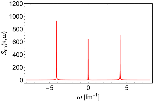
Figure 1: (Color online) The variation of the $\mathscr{S}_{nn}(\mathchoice{\mbox{\boldmath$k$}}{\mbox{\boldmath$k$}}{\mbox{\boldmath$\scriptstyle k$}}{\mbox{\boldmath$\scriptscriptstyle k$}},\omega)$ with $\omega$ is shown with magnetic field strength, $eB=m_{\pi}^{2}$ for $k=0.1$ fm^-1. It shows one R-peak and two B-peaks, symmetrically located about $\omega=0$.

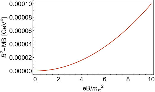
Figure 2: (Color online) The factor $B^{2}-MB$ is plotted with the variation of magnetic field.

We aim to study the nature of the dynamic structure factor [$\mathscr{S}_{nn}(\mathchoice{\mbox{\boldmath$k$}}{\mbox{\boldmath$k$}}{\mbox{\boldmath$\scriptstyle k$}}{\mbox{\boldmath$\scriptscriptstyle k$}},\omega)$] in the presence of a magnetic field, $B$. The $\mathscr{S}_{nn}(\mathchoice{\mbox{\boldmath$k$}}{\mbox{\boldmath$k$}}{\mbox{\boldmath$\scriptstyle k$}}{\mbox{\boldmath$\scriptscriptstyle k$}},\omega)$ in the absence of $B$ has been studied in earlier works Hasanujjaman et al. (2021); Sarwar et al. (2022), where it has been shown that the $\mathscr{S}_{nn}(\mathchoice{\mbox{\boldmath$k$}}{\mbox{\boldmath$k$}}{\mbox{\boldmath$\scriptstyle k$}}{\mbox{\boldmath$\scriptscriptstyle k$}},\omega)$ admits three identifiable peaks. The central Rayleigh peak (R-peak) is positioned at angular frequency $\omega=0$, and the other two peaks, the Brillouin peaks (B-peaks) are situated on both sides of the R-peak with even magnitudes. The R-peak and the B-peaks are originated from the entropy (thermal) fluctuation at constant pressure and pressure fluctuation at constant entropy respectively. The position of the B-peaks enables us to evaluate the speed of sound. Also, the width and the integrated intensities of those peaks are associated with various thermodynamic quantities such as the isothermal compressibilities and specific heats of the system Stanley (1971).

Fig. 1 shows the $\mathscr{S}_{nn}(\mathchoice{\mbox{\boldmath$k$}}{\mbox{\boldmath$k$}}{\mbox{\boldmath$\scriptstyle k$}}{\mbox{\boldmath$\scriptscriptstyle k$}},\omega)$ for $eB=m_{\pi}^{2}$. We see three different peaks which are recognized as the R-peak (central), and the other two peaks as the B-peaks. The B-peaks are positioned symmetrically about $\omega=0$, but their heights are not identical. The asymmetry (magnitude) in the B-peaks may occur due to the local inhomogeneity present in the system. The B-peaks arise from propagating sound modes associated with pressure fluctuations at constant entropy. In condensed matter physics, the asymmetry of the B-peaks is identified from the fact that two sound modes with different $\omega$ values, $-c_{s}k$ and $+c_{s}k$ originate from different temperature zones Rayleigh (1916); Zarate and Sengers (2006). Furthermore, we see that the widths of the peaks are very narrow, implying the slow relaxation rate of the thermal as well as the pressure fluctuations, which keeps the system to linger at out-of-equilibrium state for a longer time.

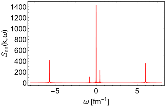
Figure 3: (Color online) The variation of the $\mathscr{S}_{nn}(\mathchoice{\mbox{\boldmath$k$}}{\mbox{\boldmath$k$}}{\mbox{\boldmath$\scriptstyle k$}}{\mbox{\boldmath$\scriptscriptstyle k$}},\omega)$ with $\omega$ is shown in the presence of a magnetic field ($B=3\,m^{2}_{\pi}$). It shows one R-peak, two away side B-peaks asymmetrically located about $\omega=0$, and two near side B-peaks, originated from the coupling of the magnetic field with the other thermodynamic fields.

The introduction of $B$ results in splitting the pressure into transverse, $P_{\perp}=P-MB$ and longitudinal, $P_{L}=P$ components. The expression of the magnetization is adapted from Ref. Huang et al. (2010). The value of $\mathscr{A}$ determines the effects of the magnetic field on the spectral function as evident from the expression of $\delta n$ in Eq. (57). Therefore, we show the variation of $\mathscr{A}=B^{2}-MB$ with $B$ in Fig. 2. The small value of $\mathscr{A}$ for low $B$ indicates that the effects of $B$ on $\mathscr{S}_{nn}(\mathchoice{\mbox{\boldmath$k$}}{\mbox{\boldmath$k$}}{\mbox{\boldmath$\scriptstyle k$}}{\mbox{\boldmath$\scriptscriptstyle k$}},\omega)$ will be significant only beyond a certain value of $B$.

The $\mathscr{S}_{nn}(\mathchoice{\mbox{\boldmath$k$}}{\mbox{\boldmath$k$}}{\mbox{\boldmath$\scriptstyle k$}}{\mbox{\boldmath$\scriptscriptstyle k$}},\omega)$ in the presence of the magnetic field $(eB=3\,m_{\pi}^{2})$ is shown in Fig. 3, where we see five distinct peaks. The peak found at $\omega=0$ is identified as the R-peak. The two distant peaks about the R-peak are recognized as the B-peaks are originated from the thermodynamic pressure fluctuation at constant entropy (longitudinal component). The magnitudes of the B-peaks are not even as well as their position about $\omega=0$ is not symmetric. The positional asymmetry could be realized due to the presence of a unidirectional magnetic field.

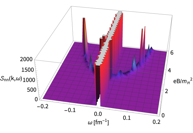
Figure 4: (Color online) A 3D plot is shown to understand the role of the magnetic field in emergence of the near side B-peaks. The peaks start appearing after a threshold value of the magnetic field, $B_{th}$.

The other two nearby peaks around the R-peak are also found to be the B-peaks due to the pressure fluctuation in the transverse direction. These B-peaks only appear in the presence of the magnetic field beyond a certain strength. The threshold value for the emergence of the B-peaks (near) is found to be at $B_{th}=2.32\,m_{\pi}^{2}$. The transverse pressure ($=P-MB$) in Eq. (39), containing the $B$ field is solely responsible for the appearance of the near side B-peaks.

The importance of the magnetic field in the appearance of those extra B-peaks is understood from Fig. 4, where the $\mathscr{S}_{nn}(\mathchoice{\mbox{\boldmath$k$}}{\mbox{\boldmath$k$}}{\mbox{\boldmath$\scriptstyle k$}}{\mbox{\boldmath$\scriptscriptstyle k$}},\omega)$ is plotted as a function of $B$. The range of $\omega$ is kept smaller to focus on the near side B-peaks only. For the smaller values of $B$, no extra peak is found, and they start appearing after a threshold value of $B_{th}$.

Fig. 5 shows the $\mathscr{S}_{nn}(\mathchoice{\mbox{\boldmath$k$}}{\mbox{\boldmath$k$}}{\mbox{\boldmath$\scriptstyle k$}}{\mbox{\boldmath$\scriptscriptstyle k$}},\omega)$ in the presence of the magnetic field in NS theory, which is recovered by putting the relaxation and coupling coefficients to be zero in the MIS theory. We see only three peaks, where the extra peaks due to the presence of the magnetic field are not appearing, but the presence of the magnetic field is evident from the magnitude as well as positional asymmetry of the B-peaks. Therefore, we argue that the extra near-side B-peaks are generated due to the coupling of hydrodynamic fields with the magnetic field when we consider second-order hydrodynamics. This is understood because the dispersion relations of MIS and NS hydrodynamics are quintic and cubic equations respectively.

The behaviour of the structure factor near the CEP is shown in Fig. 6. As the near side B-peaks appear only after a threshold intensity of the magnetic field, $B_{th}$, we have plotted the $\mathscr{S}_{nn}(\mathchoice{\mbox{\boldmath$k$}}{\mbox{\boldmath$k$}}{\mbox{\boldmath$\scriptstyle k$}}{\mbox{\boldmath$\scriptscriptstyle k$}},\omega)(k,\omega)$ for two different values of magnetic field: a) $B=m^{2}_{\pi}$, and b) $B=3\,m^{2}_{\pi}$. In both cases, we do not observe any B-peaks but only the R-peak with a larger magnitude. This happens due to the absorption of sound near the CEP, where the B-peaks merge with the R-peak. Comparing both cases, we also observe that the magnitude of the R-peak in Fig. 6(b) is larger compared to the R-peak in Fig. 6(a). The reason for the difference in magnitude in R-peak is due to the fact that at $B=3\,m^{2}_{\pi}$, the near side B-peaks originated due to the coupling of hydrodynamic fields with the magnetic field contribute to the R-peak near the CEP.

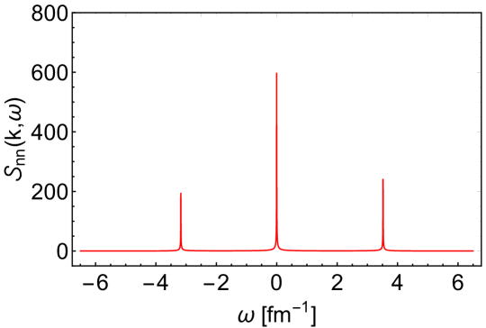
Figure 5: (Color online) The variation of the $\mathscr{S}_{nn}(\mathchoice{\mbox{\boldmath$k$}}{\mbox{\boldmath$k$}}{\mbox{\boldmath$\scriptstyle k$}}{\mbox{\boldmath$\scriptscriptstyle k$}},\omega)$ with $\omega$ is shown in the presence of a magnetic field in Navier-Stokes theory. It shows one R-peak and two away side B-peaks asymmetrically located about $\omega=0$.

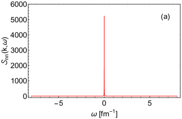
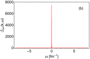
Figure 6: (Color online) The variation of the $\mathscr{S}_{nn}(\mathchoice{\mbox{\boldmath$k$}}{\mbox{\boldmath$k$}}{\mbox{\boldmath$\scriptstyle k$}}{\mbox{\boldmath$\scriptscriptstyle k$}},\omega)$ with $\omega$ near the critical end point is shown in the presence of a magnetic field in MIS theory for a) magnetic field strength $B=m^{2}_{\pi}<B_{th}$, and b) magnetic filed strength $B=3\,m^{2}_{\pi}\geq B_{th}$.

V Summary and conclusion

The dynamic structure factor, $\mathscr{S}_{nn}(\mathchoice{\mbox{\boldmath$k$}}{\mbox{\boldmath$k$}}{\mbox{\boldmath$\scriptstyle k$}}{\mbox{\boldmath$\scriptscriptstyle k$}},\omega)$, is evaluated from the correlation of the dynamical density fluctuation, when the system is subjected to an external magnetic field. Without any magnetic field, the $\mathscr{S}_{nn}(\mathchoice{\mbox{\boldmath$k$}}{\mbox{\boldmath$k$}}{\mbox{\boldmath$\scriptstyle k$}}{\mbox{\boldmath$\scriptscriptstyle k$}},\omega)$ admits a Rayleigh peak and two Brillouin peaks. But in presence of the magnetic field, we find two extra peaks appearing closer to the R-peak, and they are also identified as the B-peaks due to the adiabatic transverse pressure fluctuation. The asymmetry in magnitudes of the B-peaks (away side) are realized due to the local inhomogeneity of the system, whereas, the positional asymmetry appears due to the presence of the magnetic field. The extra B-peaks (near side) exclusively appear beyond a threshold value of the magnetic field. To understand the role of the relaxation and the coupling coefficients, we have plotted the $\mathscr{S}_{nn}(\mathchoice{\mbox{\boldmath$k$}}{\mbox{\boldmath$k$}}{\mbox{\boldmath$\scriptstyle k$}}{\mbox{\boldmath$\scriptscriptstyle k$}},\omega)$ for Navier-Stokes theory also. We find that the B-peaks (near side) are found accordingly, positioned asymmetrically with uneven magnitudes. Therefore, we argue that the near side B-peaks only appear due to the coupling of the magnetic field with the thermodynamic fields in the second-order hydrodynamic theory.

The away side and the near side B-peaks are caused by the pressure fluctuation in longitudinal and transverse direction respectively. Therefore, the presence of the near side B-peaks in the $\mathscr{S}_{nn}(\mathchoice{\mbox{\boldmath$k$}}{\mbox{\boldmath$k$}}{\mbox{\boldmath$\scriptstyle k$}}{\mbox{\boldmath$\scriptscriptstyle k$}},\omega)$ implies the pressure difference in longitudinal and transverse directions. As a result even if there is no asymmetry in the initial geometry of the collision in a heavy-ion collision (i.e. central collision), the presence of the magnetic field will create a pressure difference in the system, causing an enhancement of the various flow harmonics, specially the elliptic flow. Therefore, we argue that the enhancement of the flow harmonics in central collision could be a signature of the presence of the external magnetic field.

VI Acknowledgement

MR, MH would like to thank Department of Higher Education, Govt. of West Bengal, India for the support.

References

- Chaudhuri (2014) A.K. Chaudhuri, A short course on Relativistic Heavy Ion Collisions (IOPP, 2014) arXiv:1207.7028 [nucl-th] .
- Heinz and Snellings (2013) Ulrich Heinz and Raimond Snellings, “Collective flow and viscosity in relativistic heavy-ion collisions,” Ann. Rev. Nucl. Part. Sci. 63, 123–151 (2013), arXiv:1301.2826 [nucl-th] .
- Gale et al. (2013) Charles Gale, Sangyong Jeon, and Bjoern Schenke, “Hydrodynamic Modeling of Heavy-Ion Collisions,” Int. J. Mod. Phys. A 28, 1340011 (2013), arXiv:1301.5893 [nucl-th] .
- Romatschke and Romatschke (2019) Paul Romatschke and Ulrike Romatschke, Relativistic Fluid Dynamics In and Out of Equilibrium, Cambridge Monographs on Mathematical Physics (Cambridge University Press, 2019) arXiv:1712.05815 [nucl-th] .
- Bzdak and Skokov (2012) Adam Bzdak and Vladimir Skokov, “Event-by-event fluctuations of magnetic and electric fields in heavy ion collisions,” Phys. Lett. B 710, 171–174 (2012), arXiv:1111.1949 [hep-ph] .
- Deng and Huang (2012) Wei-Tian Deng and Xu-Guang Huang, “Event-by-event generation of electromagnetic fields in heavy-ion collisions,” Phys. Rev. C 85, 044907 (2012), arXiv:1201.5108 [nucl-th] .
- Tuchin (2013) Kirill Tuchin, “Particle production in strong electromagnetic fields in relativistic heavy-ion collisions,” Adv. High Energy Phys. 2013, 490495 (2013), arXiv:1301.0099 [hep-ph] .
- Roy and Pu (2015) Victor Roy and Shi Pu, “Event-by-event distribution of magnetic field energy over initial fluid energy density in = 200 GeV Au-Au collisions,” Phys. Rev. C 92, 064902 (2015), arXiv:1508.03761 [nucl-th] .
- Li et al. (2016) Hui Li, Xin-li Sheng, and Qun Wang, “Electromagnetic fields with electric and chiral magnetic conductivities in heavy ion collisions,” Phys. Rev. C 94, 044903 (2016), arXiv:1602.02223 [nucl-th] .
- Gupta (2004) Sourendu Gupta, “The Electrical conductivity and soft photon emissivity of the QCD plasma,” Phys. Lett. B 597, 57–62 (2004), arXiv:hep-lat/0301006 .
- Aarts et al. (2015) Gert Aarts, Chris Allton, Alessandro Amato, Pietro Giudice, Simon Hands, and Jon-Ivar Skullerud, “Electrical conductivity and charge diffusion in thermal QCD from the lattice,” JHEP 02, 186 (2015), arXiv:1412.6411 [hep-lat] .
- Amato et al. (2013) Alessandro Amato, Gert Aarts, Chris Allton, Pietro Giudice, Simon Hands, and Jon-Ivar Skullerud, “Electrical conductivity of the quark-gluon plasma across the deconfinement transition,” Phys. Rev. Lett. 111, 172001 (2013), arXiv:1307.6763 [hep-lat] .
- Huang et al. (2010) Xu-Guang Huang, Mei Huang, Dirk H. Rischke, and Armen Sedrakian, “Anisotropic Hydrodynamics, Bulk Viscosities and R-Modes of Strange Quark Stars with Strong Magnetic Fields,” Phys. Rev. D 81, 045015 (2010), arXiv:0910.3633 [astro-ph.HE] .
- Huang (2016) Xu-Guang Huang, “Electromagnetic fields and anomalous transports in heavy-ion collisions — A pedagogical review,” Rept. Prog. Phys. 79, 076302 (2016), arXiv:1509.04073 [nucl-th] .
- Greif et al. (2017) Moritz Greif, Carsten Greiner, and Zhe Xu, “Magnetic field influence on the early time dynamics of heavy-ion collisions,” Phys. Rev. C 96, 014903 (2017), arXiv:1704.06505 [hep-ph] .
- Roy et al. (2017) Victor Roy, Shi Pu, Luciano Rezzolla, and Dirk H. Rischke, “Effect of intense magnetic fields on reduced-MHD evolution in = 200 GeV Au+Au collisions,” Phys. Rev. C 96, 054909 (2017), arXiv:1706.05326 [nucl-th] .
- Gursoy et al. (2014) Umut Gursoy, Dmitri Kharzeev, and Krishna Rajagopal, “Magnetohydrodynamics, charged currents and directed flow in heavy ion collisions,” Phys. Rev. C 89, 054905 (2014), arXiv:1401.3805 [hep-ph] .
- Inghirami et al. (2016) Gabriele Inghirami, Luca Del Zanna, Andrea Beraudo, Mohsen Haddadi Moghaddam, Francesco Becattini, and Marcus Bleicher, “Numerical magneto-hydrodynamics for relativistic nuclear collisions,” Eur. Phys. J. C 76, 659 (2016), arXiv:1609.03042 [hep-ph] .
- Huang et al. (2011) Xu-Guang Huang, Armen Sedrakian, and Dirk H. Rischke, “Kubo formulae for relativistic fluids in strong magnetic fields,” Annals Phys. 326, 3075–3094 (2011), arXiv:1108.0602 [astro-ph.HE] .
- Arnold et al. (2000) Peter Brockway Arnold, Guy D. Moore, and Laurence G. Yaffe, “Transport coefficients in high temperature gauge theories. 1. Leading log results,” JHEP 11, 001 (2000), arXiv:hep-ph/0010177 .
- Arnold et al. (2003) Peter Brockway Arnold, Guy D Moore, and Laurence G. Yaffe, “Transport coefficients in high temperature gauge theories. 2. Beyond leading log,” JHEP 05, 051 (2003), arXiv:hep-ph/0302165 .
- Li and Yee (2018) Shiyong Li and Ho-Ung Yee, “Shear viscosity of the quark-gluon plasma in a weak magnetic field in perturbative QCD: Leading log,” Phys. Rev. D 97, 056024 (2018), arXiv:1707.00795 [hep-ph] .
- Cao et al. (2019) Shanshan Cao et al., “Toward the determination of heavy-quark transport coefficients in quark-gluon plasma,” Phys. Rev. C 99, 054907 (2019), arXiv:1809.07894 [nucl-th] .
- Eckart (1940) Carl Eckart, “The Thermodynamics of irreversible processes. 3.. Relativistic theory of the simple fluid,” Phys. Rev. 58, 919–924 (1940).
- Landau and Lifshitz (2013) L.D. Landau and E.M. Lifshitz, Fluid Mechanics, v. 6 (Elsevier Science, 2013).
- Hiscock and Lindblom (1983) W.A. Hiscock and L. Lindblom, “Stability and causality in dissipative relativistic fluids,” Annals Phys. 151, 466–496 (1983).
- Hiscock and Lindblom (1985) William A. Hiscock and Lee Lindblom, “Generic instabilities in first-order dissipative relativistic fluid theories,” Phys. Rev. D 31, 725–733 (1985).
- Hiscock and Lindblom (1987) William A. Hiscock and Lee Lindblom, “Linear plane waves in dissipative relativistic fluids,” Phys. Rev. D 35, 3723–3732 (1987).
- Israel (1976) W. Israel, “Nonstationary irreversible thermodynamics: A Causal relativistic theory,” Annals Phys. 100, 310–331 (1976).
- Israel and Stewart (1979) W. Israel and J.M. Stewart, “Transient relativistic thermodynamics and kinetic theory,” Annals Phys. 118, 341–372 (1979).
- Stanley (1971) H. Eugene Stanley, Introduction to phase transitions and critical phenomena (Oxford University Press, 1971).
- Minami and Kunihiro (2010) Yuki Minami and Teiji Kunihiro, “Dynamical Density Fluctuations around QCD Critical Point Based on Dissipative Relativistic Fluid Dynamics -Possible fate of Mach cone at the critical point-,” Prog. Theor. Phys. 122, 881–910 (2010), arXiv:0904.2270 [hep-th] .
- Hasanujjaman et al. (2020) Md Hasanujjaman, Mahfuzur Rahaman, Abhijit Bhattacharyya, and Jan-e Alam, “Dispersion and suppression of sound near the QCD critical point,” Phys. Rev. C 102, 034910 (2020), arXiv:2003.07575 [nucl-th] .
- Lichnerowicz and for Advanced Studies (1967) A. Lichnerowicz and Southwest Center for Advanced Studies, Relativistic Hydrodynamics and Magnetohydrodynamics, Mathematical physics monograph series (W. A. Benjamin, 1967).
- Anile (2005) A.M. Anile, Relativistic Fluids and Magneto-fluids, Cambridge Monographs on Mathematical Physics (Cambridge University Press, 2005).
- Thorne and Blandford (2017) K.S. Thorne and R.D. Blandford, Modern Classical Physics (Princeton University Press, 2017).
- De Groot (1969) S. R. De Groot, The Maxwell Equations. Non-Relativistic and Relativistic Derivations from Electron Theory (North-Holland Pub. Co., Amsterdam, 1969).
- Israel (1978) W. Israel, “The Dynamics of Polarization,” Gen. Rel. Grav. 9, 451–468 (1978).
- Gedalin (1991) M. Gedalin, “Relativistic hydrodynamics and thermodynamics of anisotropic plasmas,” Phys. Fluids B 3, 1871–1875 (1991).
- Van and Biro (2008) P. Van and T. S. Biro, “Relativistic hydrodynamics - causality and stability,” Eur. Phys. J. ST 155, 201–212 (2008), arXiv:0704.2039 [nucl-th] .
- Baier et al. (2008) Rudolf Baier, Paul Romatschke, Dam Thanh Son, Andrei O. Starinets, and Mikhail A. Stephanov, “Relativistic viscous hydrodynamics, conformal invariance, and holography,” JHEP 04, 100 (2008), arXiv:0712.2451 [hep-th] .
- Muronga (2007) Azwinndini Muronga, “Relativistic Dynamics of Non-ideal Fluids: Viscous and heat-conducting fluids. I. General Aspects and 3+1 Formulation for Nuclear Collisions,” Phys. Rev. C 76, 014909 (2007), arXiv:nucl-th/0611090 .
- Fodor and Katz (2002) Z. Fodor and S. D. Katz, “Lattice determination of the critical point of QCD at finite T and mu,” JHEP 03, 014 (2002), arXiv:hep-lat/0106002 .
- Fodor and Katz (2004) Z. Fodor and S. D. Katz, “Critical point of QCD at finite T and mu, lattice results for physical quark masses,” JHEP 04, 050 (2004), arXiv:hep-lat/0402006 .
- DeWolfe et al. (2011) Oliver DeWolfe, Steven S. Gubser, and Christopher Rosen, “A holographic critical point,” Phys. Rev. D 83, 086005 (2011), arXiv:1012.1864 [hep-th] .
- Nonaka and Asakawa (2005) Chiho Nonaka and Masayuki Asakawa, “Hydrodynamical evolution near the QCD critical end point,” Phys. Rev. C 71, 044904 (2005), arXiv:nucl-th/0410078 .
- Parotto et al. (2020) Paolo Parotto, Marcus Bluhm, Debora Mroczek, Marlene Nahrgang, Jacquelyn Noronha-Hostler, Krishna Rajagopal, Claudia Ratti, Thomas Schäfer, and Mikhail Stephanov, “QCD equation of state matched to lattice data and exhibiting a critical point singularity,” Phys. Rev. C 101, 034901 (2020), arXiv:1805.05249 [hep-ph] .
- Guida and Zinn-Justin (1997) Riccardo Guida and Jean Zinn-Justin, “3-D Ising model: The Scaling equation of state,” Nucl. Phys. B 489, 626–652 (1997), arXiv:hep-th/9610223 .
- Rajagopal and Wilczek (1993) Krishna Rajagopal and Frank Wilczek, “Static and dynamic critical phenomena at a second order QCD phase transition,” Nucl. Phys. B 399, 395–425 (1993), arXiv:hep-ph/9210253 .
- Kapusta and Torres-Rincon (2012) Joseph I. Kapusta and Juan M. Torres-Rincon, “Thermal Conductivity and Chiral Critical Point in Heavy Ion Collisions,” Phys. Rev. C 86, 054911 (2012), arXiv:1209.0675 [nucl-th] .
- Hasanujjaman et al. (2021) Md Hasanujjaman, Golam Sarwar, Mahfuzur Rahaman, Abhijit Bhattacharyya, and Jan-e Alam, “Dynamical spectral structure of density fluctuation near the QCD critical point,” Eur. Phys. J. A 57, 283 (2021), arXiv:2008.03931 [nucl-th] .
- Sarwar et al. (2022) Golam Sarwar, Md Hasanujjaman, and Jan-e Alam, “Role of slow out-of-equilibrium modes on the dynamic structure factor near the QCD critical point,” Phys. Rev. D 106, 074029 (2022), arXiv:2205.01136 [nucl-th] .
- Rayleigh (1916) Lord Rayleigh, “Lix. on convection currents in a horizontal layer of fluid, when the higher temperature is on the under side,” The London, Edinburgh, and Dublin Philosophical Magazine and Journal of Science 32, 529–546 (1916).
- Zarate and Sengers (2006) J.M.O. Zarate and J.V. Sengers, “Hydrodynamic fluctuations in fluids and fluid mixtures,” Hydrodynamic Fluctuations in Fluids and Fluid Mixtures (2006), 10.1016/B978-0-444-51515-5.X5000-5.