11institutetext: Dept. Mathematics, Faculty of Science, Stockholm University, SE-10691 Stockholm, Sweden. 11email: marc.hellmuth@math.su.se, 11email: thekkumpadan@math.su.se 22institutetext: Bioinformatics Group, Dept. Computer Science & Interdisciplinary Center for Bioinformatics, Universität Leipzig, D-04107 Leipzig, Germany. 22email: studla@bioinf.uni-leipzig.de

Fitch Graph Completion thanks: This work was supported in part by the German Research Foundation (DFG, STA 850/49-1) and the Data-driven Life Science (DDLS) program funded by the Knut and Alice Wallenberg Foundation

Marc Hellmuth 11 0000-0002-1620-5508 Peter F. Stadler 22 0000-0002-5016-5191 Sandhya Thekkumpadan Puthiyaveedu 11 0000-0002-7745-3935
Abstract

Horizontal gene transfer is an important contributor to evolution. According to Walter M. Fitch, two genes are xenologs if they are separated by at least one HGT. More formally, the directed Fitch graph has a set of genes is its vertices, and directed edges $(x,y)$ for all pairs of genes $x$ and $y$ for which $y$ has been horizontally transferred at least once since it diverged from the last common ancestor of $x$ and $y$. Subgraphs of Fitch graphs can be inferred by comparative sequence analysis. In many cases, however, only partial knowledge about the “full” Fitch graph can be obtained. Here, we characterize Fitch-satisfiable graphs that can be extended to a biologically feasible “full” Fitch graph and derive a simple polynomial-time recognition algorithm. We then proceed to showing that finding the Fitch graphs with total maximum (confidence) edge-weights is an NP-hard problem.

Keywords:
Directed Cograph Fitch Graph Horizontal Gene Transfer NP-complete Recognition Algorithm

1 Introduction

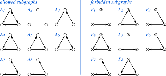
Horizontal gene transfer (HGT) is a biological process by which genes from sources other than the parents are transferred into an organisms genome. In particular in microorganism it is an important contributor to evolutionary innovation. The identification of HGT events from genomic data, however, is still a difficult problem in computational biology, both mathematically and in terms of practical applications. Recent formal results are phrased in terms of a binary relation between genes. In most situations it can be assumed that the evolution of genes is tree-like and thus can described by a gene tree $T$ whose leaves correspond to the present-day, observable genes; the interior vertices and edges then model evolutionary events such as gene duplications, speciations, and also HGT. Since HGT distinguishes between the gene copy that continues to be transmitted vertically, and the transferred copy, one associated the transfer with the edge in $T$ connecting the HGT event with its transferred offspring. Focusing on a pair of present-day genes, it is of interest to determine whether or not they have been separated by HGT events in their history. This information is captured by the Fitch (xenology) graph. It contains an edge $x\to y$ whenever a HGT event occurred between $y$ and the least common ancestor of $x$ and $y$ [6]. Fitch graphs form a hereditary sub-class of the directed cographs [4], and admit a simple characterization in terms of eight forbidden induced subgraphs on three vertices (see Fig. 1 below). Moreover, every Fitch graph uniquely determines a least resolved edge-labeled tree by which it is explained. This tree is related to the gene tree by a loss of resolution [6].

Information on HGT events can be extracted from sequence information using a broad array of methods [14], none of which is likely to yield a complete picture. Reliable information to decide whether or not two genes are xenologs, thus, may be available only for some pairs of genes $(x,y)$, but not for others. In this situation it is natural to ask whether this partial knowledge can be used to infer missing information. In [13] the analogous question was investigated for di-cographs. The main result of the present contribution is a characterization of partial Fitch graphs, Thm. 3.2, and an accompanying polynomial-time algorithm. In addition, we show that the “weighted” version of Fitch graph completion is NP-hard.

2 Preliminaries

Relations. Throughout, we consider only irreflexive, binary relations $R$ on $V$, i.e., $(x,y)\in R$ implies $x\neq y$ for all $x,y\in V$. We write $\overleftarrow{R}\coloneqq\{(x,y)\mid(y,x)\in R\}$ and $R^{\mathrm{sym}}\coloneqq R\cup\overleftarrow{R}$ for the transpose and the symmetric extension of $R$, respectively. The relation $R^{\times}_{V}\coloneqq\{(x,y)\mid x,y\in V,\,x\neq y\}$ is called the full relation. For a subset $W\subseteq V$ and a relation $R$, we define the induced subrelation as $R[W]\coloneqq\{(x,y)\mid(x,y)\in R,x,y\in W\}$. Moreover, we consider ordered tuples of relation $\mathcal{R}=(R_{1},\dots,R_{n})$. Let $R_{1},\dots,R_{n}\subseteq R^{\times}_{V}$, then $\mathcal{R}=(R_{1},\dots,R_{n})$ is full if $\cup_{i=1}^{n}R_{i}=R^{\times}_{V}$ and partial if $\cup_{i=1}^{n}R_{i}\subseteq R^{\times}_{V}$. Note that a full tuple of relations is also considered to be a partial one. Moreover, we consider component-wise sub-relation and write $\mathcal{R}[W]\coloneqq(R_{1}[W],\dots,R_{n}[W])$ and $\mathcal{R}=(R_{1},\dots,R_{n})\subseteq\mathcal{R}^{\prime}=(R^{\prime}_{1},\dots,R^{\prime}_{n})$ if $R_{i}\subseteq R^{\prime}_{i}$ holds for all $i\in\{1,\dots,n\}$. In the latter case, we say that $\mathcal{R^{\prime}}$ extends $\mathcal{R}$.

Digraphs and DAGs. A directed graph (digraph) $G=(V,E)$ comprises a vertex set $V(G)=V$ and an irreflexive binary relation $E(G)=E$ on $V$ called the edge-set of $G$. Given two disjoint digraphs $G=(V,E)$ and $H=(W,F)$, the digraphs $G\cup H=(V\cup W,E\cup F)$, $G\mathrel{\ooalign{\hss$\triangleleft$\hss\cr$\triangleright$}}H=(V\cup W,E\cup F\cup\{(x,y),(y,x)\mid x\in V,y\in W\})$ and $G\triangleright H=(V\cup W,E\cup F\cup\{(x,y)\mid x\in V,y\in W\})$ denote the union, join and directed join of $G$ and $H$, respectively. For a given subset $W\subseteq V$, the induced subgraph $G[W]=(W,F)$ of $G=(V,E)$ is the subgraph for which $x,y\in W$ and $(x,y)\in E$ implies that $(x,y)\in F$. We call $W\subseteq V$ a (strongly) connected component of $G=(V,E)$ if $G[W]$ is an inclusion-maximal (strongly) connected subgraph of $G$.

Given a digraph $G=(V,E)$ and a partition $\{V_{1},V_{2},\dots,V_{k}\}$, $k\geq 1$ of its vertex set $V$, the quotient digraph $G/\{V_{1},V_{2},\dots,V_{k}\}$ has as vertex set $\{V_{1},V_{2},\dots,V_{k}\}$ and two distinct vertices $V_{i}$ and $V_{j}$ form an edge $(V_{i},V_{j})$ in $G/\{V_{1},\dots,V_{k}\}$ if there are vertices $x\in V_{i}$ and $y\in V_{j}$ with $(x,y)\in E$. Note, that edges $(V_{i},V_{j})$ in $G/\{V_{1},\dots,V_{k}\}$ do not necessarily imply that $(x,y)$ form an edge in $G$ for $x\in V_{i}$ and $y\in V_{j}$. Nevertheless, at least one such edge $(x,y)$ with $x\in V_{i}$ and $y\in V_{j}$ must exist in $G$ given that $(V_{i},V_{j})$ is an edge in $G/\{V_{1},\dots,V_{k}\}$

A cycle $C$ in a digraph $G=(V,E)$ of length $n$ is an ordered sequence of $n>1$ (not necessarily distinct) vertices $(v_{1},\dots,v_{n})$ such that $(v_{n},v_{1})\in E$ and $(v_{i},v_{i+1})\in E$, $1\leq i<n$. A digraph that does contain cycles is a DAG (directed acyclic graph). Define the relation $\preceq_{G}$ of $V$ such that $v\preceq_{G}w$ if there is directed path from $w$ to $v$. A vertex $x$ is a parent of $y$ if $(x,y)\in E$. In this case $y$ is child of $x$. Then $G$ is DAG if and only if $\preceq_{G}$ is a partial order. We write $y\prec_{T}x$ if $y\preceq_{T}x$ and $x\neq y$. A topological order of $G$ is a total order $\ll$ on $V$ such that $(v,w)\in E$ implies that $v\ll w$. It is well known that a digraph $G$ admits a topological order if and only if $G$ is a DAG. In this case, $x\prec_{G}y$ implies $y\ll x$, i.e., $\ll$ is a linear extension of $\prec$. Note that $\preceq$ and $\ll$ are arranged in opposite order. The effort to check whether $G$ admits a topological order $\ll$ and, if so, to compute $\ll$ is linear, i.e., in $O(|V|+|E|)$ [10]. If $C_{1},\dots,C_{k}$, $k\geq 1$ are the strongly connected components of a directed graph, then $G/\{C_{1},C_{2},\dots,C_{k}\}$ is a DAG.

A DAG $G$ is rooted if it contains a unique $\preceq_{G}$-maximal element $\rho_{G}$ called the root. Note that $\rho_{G}$ is $\ll$-minimal. A rooted tree $T$ with vertex set $V(T)$ is a DAG such that every vertex $x\in V(T)\setminus\{\rho_{T}\}$ has a unique parent. The rooted trees considered here do not contain vertices $v$ with $\mathrm{indeg}(v)=\mathrm{outdeg}(v)=1$. A vertex $x$ is an ancestor of $y$ if $x\preceq_{T}y$, i.e., if $x$ is located on the unique path from $\rho_{T}$ to $y$. A vertex in $T$ without a child is a leaf. The set of leaves of $T$ will be denoted by $L(T)$. The elements in $V^{0}(T)\coloneqq V(T)\setminus L(T)$ are called the inner vertices. We write $T(u)$ for the subtree of $T$ induced by $\{v\in V(T)\mid v\preceq_{T}u\}$. Note that $u$ is the root of $T(u)$.

For a subset $W\subseteq L(T)$, the least common ancestor $\operatorname{lca}_{T}(W)$ of $W$ is the unique $\preceq_{T}$-minimal vertex that is an ancestor of each $w\in W$. If $W=\{x,y\}$, we write $\operatorname{lca}_{T}(x,y)\coloneqq\operatorname{lca}_{T}(\{x,y\})$. A rooted tree $T$ is ordered, if the children of every vertex in $T$ are ordered.

We say that rooted trees $T_{1},\dots,T_{k}$, $k\geq 2$ are joined under a new root in the tree $T$ if $T$ is obtained by the following procedure: add a new root $\rho_{T}$ and all trees $T_{1},\dots,T_{k}$ to $T$ and connect the root $\rho_{T_{i}}$ of each tree $T_{i}$ to $\rho_{T}$ with an edge $(\rho_{T},\rho_{T_{i}})$.

Directed Cographs. Di-cographs generalize the notion of undirected cographs [5, 4, 2, 3] and are defined recursively as follows: (i) the single vertex graph $K_{1}$ is a di-cograph, and (ii) if $G$ and $H$ are di-cographs, then $G\cup H$, $G\mathrel{\ooalign{\hss$\triangleleft$\hss\cr$\triangleright$}}H$, and $G\triangleright H$ are di-cographs [7, 13]. Every di-cograph $G=(V,E)$ is explained by an ordered rooted tree $T=(W,F)$, called a cotree of $G$, with leaf set $L(T)=V$ and a labeling function $t:W^{0}\to\{0,1,\overrightarrow{1}\}$ that uniquely determines the set of edges $E(G)=E_{1}(T,t)\cup E_{\overrightarrow{1}}(T,t)$ and set of non-edges $E_{0}(T,t)$ of $G$ as follows:

$\displaystyle E_{1}(T,t)=\{(x,y)\mid t(\operatorname{lca}(x,y))=1\},$
$\displaystyle E_{0}(T,t)=\{(x,y)\mid t(\operatorname{lca}(x,y))=0\},\text{ and}$
$\displaystyle E_{\overrightarrow{1}}(T,t)=\{(x,y)\mid t(\operatorname{lca}(x,y))=\overrightarrow{1}\text{ and }x\text{ is left of }y\text{ in }T\}.$

Note that $E_{i}(T,t)=E_{i}(T,t)^{\mathrm{sym}}$ for $i\in\{0,1\}$ since $\operatorname{lca}(x,y)=\operatorname{lca}(y,x)$. Every di-cograph $G=(V,E)$ is explained by a unique discriminating cotree $(T,t)$ satisfying $t(x)\neq t(y)$ for all $(x,y)\in E(T)$. Every cotree $(T^{\prime},t^{\prime})$ that explains $G$ is “refinement” of it discriminating cotree $(T,t)$, i.e., $(T,t)$ is obtained by contracting all edges $(x,y)\in E(T^{\prime})$ with $t^{\prime}(x)=t^{\prime}(y)$ [1]. Determining whether a digraph is a di-cograph, and if so, computing its discriminating cotree requires $O(|V|+|E|)$ time [2, 7, 12].

3 Fitch graphs and Fitch-satisfiability

Basic properties of Fitch graphs.

Fitch Graphs are defined in terms of edge-labeled rooted trees $T$ with an edge-labeling $\lambda\colon E\to\{0,1\}$ and leaf set $L(T)=V$. The graph $\mathbb{G}(T,\lambda)=(V,E)$ contains an edge $(x,y)$ for $x,y\in V$ if and only if the (unique) path from $\operatorname{lca}_{T}(x,y)$ to $y$ contains at least one edge $e\in E(T)$ with label $\lambda(e)=1$. The edge set of $\mathbb{G}(T,\lambda)$ by construction is a binary irreflexive relation on $V$. A directed graph $G$ is a Fitch graph if there is a tree $(T,\lambda)$ such that $G\simeq\mathbb{G}(T,\lambda)$. Fitch graphs form a proper subset of directed cographs [6]. Therefore, they can be explained by a cotree.

Refer to caption
Figure 1: Of the 16 possible irreflexive binary relations on three vertices, eight ($A_{1}$ through $A_{8}$) may appear in Fitch graphs, while the remaining eight ($F_{1}$ through $F_{8}$) form forbidden induced subgraphs.
Definition 1

A cotree $(T,t)$ is a Fitch-cotree if there are no two vertices $v,w\in V^{0}(T)$ with $w\prec_{T}v$ such that either (i) $t(v)=0\neq t(w)$ or (ii) $t(v)=\overrightarrow{1}$, $t(w)=1$, and $w\in V(T(u))$ where $u$ is a child of $v$ distinct from the right-most child of $v$.

In other words, a Fitch-cotree satisfies:

  • (a)

    No vertex with label 00 has a descendant with label $1$ or $\overrightarrow{1}$.

  • (b)

    If a vertex $v$ has label $\overrightarrow{1}$, then the subtree $T(u)$ rooted at a $u$ child of $v$ — except the right-most one — does not contain vertices with label $1$. In particular, if $T$ is discriminating, then $T(u)$ is either a star-tree whose root $u$ has label $t(u)=0$ or $u$ is a leaf. In either case, the di-cograph $G[L(T(u))]$ defined by the subtree $T(u_{1})$ of left-most child $u_{1}$ of $v$, is edge-less.

Fitch graphs have several characterizations that will be relevant throughout this contribution. We summarize [8, L. 2.1] and [6, Thm. 2] in the following

Theorem 3.1

For every digraph $G=(V,E)$ the following statements are equivalent.

  1. 1.

    $G$ is a Fitch graph.

  2. 2.

    $G$ does not contain an induced $F_{1},F_{2},\dots,F_{8}$ (cf. Fig. 1).

  3. 3.

    $G$ is a di-cograph that does not contain an induced $F_{1}$, $F_{5}$ and $F_{8}$ (cf. Fig. 1).

  4. 4.

    $G$ is a di-cograph that is explained by a Fitch-cotree.

  5. 5.

    Every induced subgraph of $G$ is a Fitch graph, i.e., the property of being a Fitch graph is hereditary.

Fitch graphs can be recognized in $O(|V|+|E|)$ time. In the affirmative case, the (unique least-resolved) edge-labeled tree $(T,\lambda)$ can be computed in $O(|V|)$ time.

Alternative characterizations can be found in [9]. The procedure cotree2fitchtree described in [6] can be used to transform a Fitch cotree $(T,t)$ that explains a Fitch graph $G$ into an edge-labeled tree $(T^{\prime},\lambda)$ that explains $G$ in $O(|V(T)|)$ time, avoiding the construction of the di-cograph altogether. For later reference, we provide the following simple results.

Lemma 1

The graph obtained from a Fitch graph by removing all bi-directional edges is a DAG.

Proof

Let $G=(V,E)$ be the graph obtained from the Fitch graph $F$ by removing all bi-directional edges and assume, for contradiction, that $G$ is not acyclic. Hence, there is a smallest cycle $C=(v_{1},\dots,v_{n})$ in $G$ with $n\geq 3$ vertices. If $n=3$, then $G$ contains $F_{2}$ as an induced subgraph and thus, $F_{2}$ is an induced subgraph of $F$. This contradicts Thm. 3.1 and thus the assumption that $F$ is a Fitch graph. Hence, $n>3$ must hold. Now consider $v_{1},v_{2}$ and $v_{3}$ on $C$ with edges $(v_{1},v_{2}),(v_{2},v_{3})\in E$. Since $G$ does not contain cycles on three vertices, we have $(v_{3},v_{1})\notin E$ and either $(v_{1},v_{3})\in E$ or $(v_{1},v_{3})\notin E$. If $(v_{1},v_{3})\in E$, then $G$ contains a smaller cycle $(v_{1},v_{3},\dots,v_{n})$; a contradiction to the choice of $C$ as a shortest cycle. Hence, $(v_{1},v_{3})\notin E$ must hold. This leaves two cases for $F$:

  1. 1.

    $(v_{1},v_{3}),(v_{3},v_{1})\in E(F)$. In this case $v_{1}$, $v_{2}$ and $v_{3}$ induce an $F_{4}$ in $F$;

  2. 2.

    $(v_{1},v_{3}),(v_{3},v_{1})\notin E(F)$, i.e., $v_{1}$ and $v_{3}$ are not adjacent in $F$. In this case $v_{1}$, $v_{2}$ and $v_{3}$ induce an $F_{3}$ in $F$.

Both alternatives contradict the assumption that $F$ is a Fitch graph. Thus $G$ must be acyclic. ∎

Corollary 1

Every Fitch graph without bi-directional edges is a DAG.

Removal of the bi-directional edges from the Fitch graph $A_{6}$ yields the graph $F_{1}$, i.e., although removal of all bi-directional edges from Fitch graphs yields a DAG it does not necessarily result in a Fitch graph.

Corollary 2

Let $G$ be a directed graph without non-adjacent pairs of vertices and no bi-directional edges. Then, $G$ is a Fitch graph if and only if it is a $DAG$.

Proof

Suppose that $G$ is a directed graph without non-adjacent pairs of vertices and no bi-directional edges. Hence, $G$ cannot contain the forbidden subgraphs $F_{1}$ and $F_{3},\dots,F_{8}$. If $G$ is a DAG, it also cannot contain $F_{2}$. Thus Thm. 3.1 implies that $G$ a Fitch graph. Conversely, if $G$ is a Fitch graph without bidirectional edges, then Cor. 1 implies that $G$ is a DAG. ∎

Characterizing Fitch-satisfiability.

Throughout we consider 3-tuples of (partial) relations $\mathcal{E}=(E_{0},E_{1},E_{\overrightarrow{1}})$ on $V$ such that $E_{0}$ and $E_{1}$ are symmetric and $E_{\overrightarrow{1}}$ is antisymmetric.

Definition 2 (Fitch-sat)

$\mathcal{E}$ is Fitch-satisfiable (in short Fitch-sat), if there is a full tuple $\mathcal{E}^{*}=\{E^{*}_{0},E^{*}_{1},E^{*}_{\overrightarrow{1}}\}$ (with $E^{*}_{0}$ and $E^{*}_{1}$ being symmetric and $E^{*}_{\overrightarrow{1}}$ being antisymmetric) that extends $\mathcal{E}$ and that is explained by a Fitch-cotree $(T,t)$.

By slight abuse of notation, we also say that, in the latter case, $\mathcal{E}$ is explained by $(T,t)$. The problem of finding a tuple $\mathcal{E}^{*}$ that extends $\mathcal{E}$ and that is explained by an arbitrary cotree was investigated in [13]. Thm. 3.1 together with the definition of cotrees and Def. 2 implies

Corollary 3

$\mathcal{E}=(E_{0},E_{1},E_{\overrightarrow{1}})$ on $V$ is Fitch-sat precisely if it can be extended to a full tuple $\mathcal{E}^{*}=(E^{*}_{0},E^{*}_{1},E^{*}_{\overrightarrow{1}})$ for which $H=(V,E^{*}_{1}\cup E^{*}_{\overrightarrow{1}})$ is a Fitch graph. In particular, there is a discriminating Fitch-cotree that explains $\mathcal{E}$, $\mathcal{E}^{*}$, and $H$.

Fitch-satisfiability is a hereditary graph property.

Lemma 2

A partial tuple $\mathcal{E}$ on $V$ is Fitch-sat if and only if $\mathcal{E}[W]$ is Fitch-sat for all $W\subseteq V$.

Proof

The if direction follows from the fact that $\mathcal{E}[W]$ is Fitch-sat for $W=V$ because $\mathcal{E}[V]=\mathcal{E}$. For the only-if direction let $W\subseteq V$ and assume that $\mathcal{E}=(E_{0},E_{1},E_{\overrightarrow{1}})$ is Fitch-sat. By Cor. 3), $\mathcal{E}$ can be extended to a full 3-tuple $\mathcal{E}^{*}=(E^{*}_{0},E^{*}_{1},E^{*}_{\overrightarrow{1}})$ for which $(V,E^{*}_{1}\cup E^{*}_{\overrightarrow{1}})$ is a Fitch graph. Since the property of being a Fitch graph is a hereditary (Thm. 3.1), $(W,E^{*}_{1}[W]\cup E^{*}_{\overrightarrow{1}}[W])$ is again a Fitch graph. Moreover, we have $E^{*}_{0}[W]=R^{\times}_{W}\setminus(E^{*}_{1}[W]\cup E^{*}_{\overrightarrow{1}}[W]))$, $E_{0}[W]\subseteq E^{*}_{0}[W]$, $E_{1}[W]\subseteq E^{*}_{1}[W]$, and $E_{\overrightarrow{1}}[W]\subseteq E^{*}_{\overrightarrow{1}}[W]$, and thus $\mathcal{E}^{*}[W]=(E^{*}_{0}[W],E^{*}_{1}[W],E^{*}_{\overrightarrow{1}}[W])$ is a full tuple that extends $\mathcal{E}[W]$. In summary, $\mathcal{E}[W]$ is Fitch-sat. ∎

For the proof of Theorem 3.2, we will need the following technical result.

Lemma 3

Let $\mathcal{E}=(E_{0},E_{1},E_{\overrightarrow{1}})$ be a Fitch-sat partial tuple on $V$ that it is explained by the discriminating Fitch-cotree $(T,t)$ and put $G_{0}[W]\coloneqq(W,E_{1}[W]\cup E_{\overrightarrow{1}}[W])$ for $W\subseteq V$. If there is a vertex $u\in V^{0}(T)$ such that $t(u)=0$, then $G_{0}[C]$ is edge-less for all $C\subseteq L(T(u))$.

Proof

Suppose that $\mathcal{E}=(E_{0},E_{1},E_{\overrightarrow{1}})$ on $V$ is Fitch-sat and let $\mathcal{E}^{*}=(E_{0}^{*},E_{1}^{*},E_{\overrightarrow{1}}^{*})$ be the full tuple that is explained by the discriminating Fitch-cotree $(T,t)$ and that extends $\mathcal{E}$. Assume that there is a vertex $u\in V^{0}(T)$ such that $t(u)=0$. Put $W\coloneqq L(T(u))$. Since $(T,t)$ is a Fitch-cotree, there is no inner vertex $v$ such that $v\prec_{T}u$ and $t(v)\neq 0$. Therefore, and because $(T,t)$ is discriminating, all vertices $v\prec_{T}u$ must be leaves. This implies that for all distinct $x,y\in W$ it holds that $\operatorname{lca}(x,y)=u$ and, thus, $t(\operatorname{lca}(x,y))=t(u)=0$. Since $(T,t)$ explains $\mathcal{E}^{*}$ it follows that $E_{0}^{*}[W]=R^{\times}_{W}$ and, thus, $E_{1}^{*}[W]=E_{\overrightarrow{1}}^{*}[W]=\emptyset$. Since $E_{1}[W]\subseteq E_{1}^{*}[W]$ and $E_{\overrightarrow{1}}[W]\subseteq E^{*}_{\overrightarrow{1}}[W]$, we have $E_{1}[W]=E_{\overrightarrow{1}}[W]=\emptyset$. Hence, $G_{0}[W]=(W,E_{1}[W]\cup E_{\overrightarrow{1}}[W])$ is edge-less. Trivially, $G_{0}[C]$ must be edge-less for all $C\subseteq W$. ∎

We are now in the position to provide a characterization of Fitch-sat partial tuples.

Theorem 3.2

The partial tuple $\mathcal{E}=(E_{0},E_{1},E_{\overrightarrow{1}})$ on $V$ is Fitch-sat if and only if at least one of the following statements hold.

(S1)

$G_{0}\coloneqq(V,E_{1}\cup E_{\overrightarrow{1}})$ is edge-less.

(S2)

(a) $G_{1}\coloneqq(V,E_{0}\cup E_{\overrightarrow{1}})$ is disconnected and

(b) $\mathcal{E}[C]$ is Fitch-sat for all connected components $C$ of $G_{1}$

(S3)
(a)(I)

$G_{\overrightarrow{1}}\coloneqq(V,E_{0}\cup E_{1}\cup E_{\overrightarrow{1}})$ contains $k>1$ strongly connected

components $C_{1},\dots,C_{k}$ collected in $\mathcal{C}$ and

   (II)

there is a $C\in\mathcal{C}$ for which the following conditions are satisfied:

  (i)

$G_{0}[C]$ is edge-less.

  (ii)

$C$ is $\ll$-minimal for some topological order $\ll$

on $G_{\overrightarrow{1}}/\{C_{1},C_{2},\dots,C_{k}\}$.

  (b)

$\mathcal{E}[V\setminus C]$ is Fitch-sat.

Proof

We start with proving the if direction and thus assume that $\mathcal{E}=(E_{0},E_{1},E_{\overrightarrow{1}})$ is a partial tuple on $V$ that satisfies at least one of (S1), (S2) and (S3).

First assume that $\mathcal{E}$ satisfies (S1). Hence, $G_{0}\coloneqq(V,E_{1}\cup E_{\overrightarrow{1}})$ is edge-less and we can replace $E_{0}$ by $E_{0}^{*}\coloneqq R^{\times}_{V}$ to obtain the full tuple $\mathcal{E}^{*}=(E_{0}^{*},E_{1},E_{\overrightarrow{1}})=(R^{\times}_{V},\emptyset,\emptyset)$. One easily verifies that the star tree with leaf-set $V$ and whose root is labeled “0” explains $\mathcal{E}^{*}$ and is, in particular, a Fitch-cotree. Hence, $\mathcal{E}^{*}$ is Fitch-sat.

Next assume that $\mathcal{E}$ satisfies (S2). Hence, $G_{1}\coloneqq(V,E_{0}\cup E_{\overrightarrow{1}})$ is disconnected and $\mathcal{E}[C_{i}]$ is Fitch-sat for each connected component $C_{1},\dots,C_{k}$, $k>1$. Thus, we can extend each $\mathcal{E}[C_{i}]$ to a full sat $\mathcal{E}^{*}[C_{i}]$ that is explained by a Fitch-cotree $(T_{i},t_{i})$. Let $\mathcal{E}^{\prime}=(E^{*}_{0},E^{\prime}_{1},E^{*}_{\overrightarrow{1}})$ be the resulting partial tuple obtained from $\mathcal{E}$ such that $E^{*}_{0}=E_{0}\cup(\cup_{i=1}^{k}E^{*}_{0}[C_{i}])$, $E^{\prime}_{1}=E_{1}\cup(\cup_{i=1}^{k}E^{*}_{1}[C_{i}])$, and $E^{*}_{\overrightarrow{1}}=E_{\overrightarrow{1}}\cup(\cup_{i=1}^{k}E^{*}_{\overrightarrow{1}}[C_{i}])$. To obtain $E^{*}_{0}$ and $E^{*}_{\overrightarrow{1}}$, we added only pairs $(x,y)$ with $x,y\in C_{i}$ to $E_{0}$ and $E_{\overrightarrow{1}}$, respectively. Therefore, $G^{*}_{1}\coloneqq(V,E^{*}_{0}\cup E^{*}_{\overrightarrow{1}})$ remains disconnected and has, in particular, connected component $C_{1},\dots,C_{k}$. We now extend $\mathcal{E}^{\prime}$ to a full tuple $\mathcal{E}^{*}$ by adding all $(x,y)\in R^{\times}_{V}\setminus(E^{*}_{0}\cup E^{\prime}_{1}\cup E^{*,\mathrm{sym}}_{\overrightarrow{1}})$ to $E^{\prime}_{1}$ to obtain $E^{*}_{1}$. Note that the pairs in $E^{*}_{1}$ do not alter disconnectedness of $G^{*}_{1}$, i.e., $G^{*}_{1}$ has still connected components $C_{1},\dots C_{k}$. By construction, we have $(x,y)\in E^{*}_{1}\setminus(\cup_{i=1}^{k}E^{*}_{1}[W])$ with $W=\cup_{i=1}^{k}C_{i}$ if and only if $x$ and $y$ are in distinct connected components of $G^{*}_{1}$. We know join the Fitch-cotrees $(T_{1},t_{1}),\dots(T_{k},t_{k})$ under a common root $\rho$ with label “1” and keep the labels of all other vertices to obtain the cotree $(T,t)$. Since each $(T_{i},t_{i})$ is a Fitch-cotree and since no constraints are imposed on vertices with label label “1” (and thus on the root $\rho$ of $T$), it follows that $(T,t)$ is a Fitch-cotree. Moreover, by construction, for all $x$ and $y$ that are in distinct connected components of $G^{*}_{1}$ we have $\operatorname{lca}_{T}(x,y)=\rho$ and thus $t(\operatorname{lca}_{T}(x,y))=1$. Hence, $(x,y)\in E^{*}_{1}\setminus(\cup_{i=1}^{k}E^{*}_{1}[W]$ if and only of $\operatorname{lca}_{T}(x,y)=\rho$ and thus $t(\operatorname{lca}_{T}(x,y))=1$. Moreover, each Fitch-cotree $(T_{i},t_{i})$ explains $\mathcal{E}^{*}[C_{i}]$. Taken the latter arguments together, the Fitch-cotree $(T,t)$ explains the full tuple $\mathcal{E}^{*}$, and thus $\mathcal{E}$ is Fitch-sat.

Finally, assume that $\mathcal{E}$ satisfies (S3). By (S3.a.I), $G_{\overrightarrow{1}}\coloneqq(V,E_{0}\cup E_{1}\cup E_{\overrightarrow{1}})$ has $k>1$ strongly connected components $C_{1},\dots,C_{k}$ collected in $\mathcal{C}$. Moreover, by (S3.a.II.i), there is a $C\in\mathcal{C}$ for which $G_{0}[C]$ is edge-less, where $C$ is $\ll$-minimal for some topological order $\ll$ on $G_{\overrightarrow{1}}/\{C_{1},C_{2},\dots,C_{k}\}$ and where $\mathcal{E}[\widehat{C}]$ is Fitch-sat for $\widehat{C}=V\setminus C$. Since $\mathcal{E}[\widehat{C}]$ is Fitch-sat, $\mathcal{E}[\widehat{C}]$ can be extended to a full tuple $\mathcal{E}^{*}[\widehat{C}]=(E^{*}_{0}[\widehat{C}],E^{*}_{1}[\widehat{C}],E^{*}_{\overrightarrow{1}}[\widehat{C}])$ that is a explained by a Fitch-cotree $(\widehat{T},\widehat{t})$. Moreover, $G_{0}[C]$ is edge-less and thus $\mathcal{E}[C]=(E_{0}[C],E_{1}[C],E_{\overrightarrow{1}}[C])=(E_{0}[C],\emptyset,\emptyset)$. We can now extend $\mathcal{E}[C]$ to a full tuple $\mathcal{E}^{*}[C]=(E^{*}_{0}[C],\emptyset,\emptyset)$ by adding all pairs $(x,y)\in R^{\times}_{C}\setminus C$ to $E_{0}[C]$. Clearly, $G^{*}_{0}[C]$ remains edge-less. Hence, $\mathcal{E}^{*}[C]$ is explains by the Fitch-cotree $(T^{\prime},t^{\prime})$ where $T^{\prime}$ is a star-tree whose root $\rho_{T^{\prime}}$ has label $t^{\prime}(\rho_{T^{\prime}})=0$. We finally join $(T^{\prime},t^{\prime})$ and $(\widehat{T},\widehat{t})$ under a common root $\rho_{T}$ with to obtain the cotree $(T,t)$ where we put $t(\rho_{T})=\overrightarrow{1}$ and assume that $\rho_{T^{\prime}}$ is placed left of $\rho_{\widehat{T}}$. The latter, in particular, ensures that $(T,t)$ is a Fitch-cotree.

It remains to show that the full-set $\mathcal{E}^{*}$ explained by $(T,t)$ extends $\mathcal{E}$. First observe that, by construction, $E_{\wr}[C]\subseteq E^{*}_{\wr}[C]$ and $E_{\wr}[\widehat{C}]\subseteq\ E^{*}_{\wr}[\widehat{C}]$ for $\wr\in\{0,1,\overrightarrow{1}\}$. By construction of $(T,t)$, we have $\operatorname{lca}_{T}(x,y)=\rho_{T}$ for all $x\in C$ and $y\in\widehat{C}$. By construction, $(T,t)$ explains $\mathcal{E}^{*}[C]$ and $\mathcal{E}^{*}[\widehat{C}]$ and thus, $\mathcal{E}^{*}[C]$ extends $\mathcal{E}[C]$ while and $\mathcal{E}^{*}[\widehat{C}]$ extends $\mathcal{E}[\widehat{C}]$.

Hence, it remains to consider all vertices $x\in C$ and $y\in\widehat{C}$. Let $x\in C$ and $y\in\widehat{C}$. Since $C$ is $\ll$-minimal for some topological order $\ll$ on $H\coloneqq G_{\overrightarrow{1}}/\{C_{1},C_{2},\dots,C_{k}\}$, there is no edge $(C^{\prime},C)$ in $H$ for any $C^{\prime}\in\mathcal{C}$ with $C^{\prime}\subseteq\widehat{C}$. Hence, there is no edge $(y,x)$ in $G_{\overrightarrow{1}}$. Therefore, any edge between $x$ and $y$ that is contained in a relation of $\mathcal{E}$ must satisfy $(x,y)\in E_{\overrightarrow{1}}$ (since $E_{0}$ and $E_{1}$ are symmetric). Since $\rho_{T^{\prime}}$ is placed left of $\rho_{\widehat{T}}$, it follows that $x\in C$ is placed left of $y\in C^{\prime}$ for every $C^{\prime}\subseteq\widehat{C}$. This, together with the fact that $\operatorname{lca}_{T}(x,y)=\rho_{T}$ and $t(\rho_{T})=\overrightarrow{1}$, implies that $(x,y)\in E_{\overrightarrow{1}}$ is correctly explained for all $x\in C$ and $y\in\widehat{C}$. Moreover, for every $x\in C$ and $y\in\widehat{C}$, we have by construction of $(T,t)$ that $(x,y)\in E^{*}_{\overrightarrow{1}}$ and $(y,x)\notin E^{*}_{\overrightarrow{1}}$. Hence, $E_{\overrightarrow{1}}\subseteq E^{*}_{\overrightarrow{1}}$ holds. Thus, the full-set $\mathcal{E}^{*}$ that is explained by $(T,t)$ extends $\mathcal{E}$ and, therefore, $\mathcal{E}$ is Fitch-sat.

For the only-if direction, we assume that the partial tuple $\mathcal{E}=(E_{0},E_{1},E_{\overrightarrow{1}})$ on $V$ is Fitch-sat. If $|V|=1$, then (S1) is obviously satisfied. We therefore assume $|V|\geq 2$ from here on. Let $\mathcal{E}^{*}=(E_{0}^{*},E_{1}^{*},E_{\overrightarrow{1}}^{*})$ be a full tuple that is Fitch-sat and that extends $\mathcal{E}$. By Cor. 3, there is a discriminating Fitch-cotree $(T,t)$ endowed with the sibling order order $<$ that explains $\mathcal{E}$ and $\mathcal{E}^{*}$ and has leaf set $V$. Moreover, the root $\rho$ of $T$ has at $r\geq 2$ children $v_{1},\dots,v_{r}$ ordered from left to right according to $<$ and has one of the three labels $0,1,\overrightarrow{1}$. In the following, $L_{i}=\{x\in L(T)\mid x\preceq v_{i}\}$ denotes the set of all leaves $x$ of $T$ with $x\preceq v_{i}$. We make frequent use of the fact that $\operatorname{lca}(x,y)=\rho$ and thus, $t(\operatorname{lca}(x,y))=t(\rho)$ for all $x\in L_{i},y\in L_{j}$ with $i\neq j$ without further notice. We proceed by considering the three possible choices of $t(\rho)$.

If $t(\rho)=0$, then Lemma 3 implies that $G_{0}=(V,E_{1}\cup E_{\overrightarrow{1}})$ is edge-less and thus $\mathcal{E}$ satisfies (S1). If $t(\rho)=1$, then $t(\rho)=t(\operatorname{lca}(x,y))=1$ for all $x\in L_{i},y\in L_{j}$ with $i\neq j$. Hence, $G_{1}^{*}=(V,E^{*}_{0}\cup E_{\overrightarrow{1}}^{*})$ must be disconnected. Since $E_{0}\subseteq E_{0}^{*}$ and $E_{\overrightarrow{1}}\subseteq E^{*}_{\overrightarrow{1}}$, $G_{1}=(V,E_{0}\cup E_{\overrightarrow{1}})$ is a subgraph of $G^{*}_{1}$ and thus, $G_{1}$ is also disconnected. For each of the connected components $C$ of $G_{1}$, Lemma 2 implies that $\mathcal{E}[C]$ is Fitch-sat. Therefore, $\mathcal{E}$ satisfies (S2).

If $t(\rho)=\overrightarrow{1}$ we have $t(\operatorname{lca}(x,y))=\overrightarrow{1}$ for all $x\in L_{i}$, $y\in L_{j}$ with $i\neq j$. Since $(T,t)$ explains $\mathcal{E}^{*}$, we observe that $(x,y)\in E^{*}_{\overrightarrow{1}}$ and $(y,x)\notin E^{*}_{\overrightarrow{1}}$ for all $x\in L_{i}$, $y\in L_{j}$ with $1\leq i<j\leq r$. Thus, $G^{*}_{\overrightarrow{1}}\coloneqq(V,E^{*}_{0}\cup E^{*}_{1}\cup E^{*}_{\overrightarrow{1}})=G^{*}_{\overrightarrow{1}}[L_{1}]\triangleright\dots\triangleright G^{*}_{\overrightarrow{1}}[L_{r}]$. Hence, $G^{*}_{\overrightarrow{1}}$ contains more than one strongly connected component (which may consist of a single vertex). In particular, each strongly connected component of $G^{*}_{\overrightarrow{1}}$ must be entirely contained in some $L_{i}$, $i\in\{1,\dots,r\}$. Let $\mathcal{C}$ be the set of strongly connected components of $G_{\overrightarrow{1}}$. Since $G_{\overrightarrow{1}}$ is a subgraph of $G^{*}_{\overrightarrow{1}}$, $G_{\overrightarrow{1}}$ contains more than one strongly connected component and therefore, $\mathcal{E}$ satisfies (S3.a.I). In particular, each $C\in\mathcal{C}$ must be contained in some strongly connected component of $G^{*}_{\overrightarrow{1}}$. Taken the latter arguments together, each $C\in\mathcal{C}$ must satisfy $C\subseteq L_{i}$ for some $i\in\{1,\dots,r\}$.

Consider now the left-most child $v_{1}$ of $\rho$. Since $(T,t)$ is a discriminating Fitch-cotree, this vertex $v_{1}$ is either a leaf of $T$ or $t(v_{1})=0$. In either case, $G_{0}[L_{1}]$ is edge-less (cf. Lemma 3). By the latter arguments and since $L_{1}\neq\emptyset$, there is some $C\in\mathcal{C}$ with $C\subseteq L_{1}$. Since $G_{0}[C]\subseteq G_{0}[L_{1}]$ is edge-less, Condition (S3.a.II.i) holds.

Let $C^{\prime}\in\mathcal{C}\setminus\{C\}$. Suppose first that $C^{\prime}\subseteq L_{1}$. Assume, for contradiction, that there are edges $(x,y)$ or $(y,x)$ with $x\in C$ and $y\in C^{\prime}$ in $G_{\overrightarrow{1}}$. Since $G_{0}[L_{1}]$ is edge-less, we have $(x,y)\in E_{0}$ or $(y,x)\in E_{0}$. Since $E_{0}$ is symmetric $(x,y)\in E_{0}$ implies $(y,x)\in E_{0}$ and vice versa. Hence, the union $C\cup C^{\prime}$ would be strongly connected in $G_{\overrightarrow{1}}$; a contradiction since $C$ and $C^{\prime}$ are distinct. Hence, there cannot be any edge between vertices in $C$ and $C^{\prime}$ in $G_{\overrightarrow{1}}$ whenever $C^{\prime}\subseteq L_{1}$. Suppose now that $C^{\prime}\subseteq L_{i}$, $1<i\leq r$. As argued above, $(x,y)\in E^{*}_{\overrightarrow{1}}$ and $(y,x)\notin E^{*}_{\overrightarrow{1}}$ for all $x\in C\subseteq L_{1}$ and $y\in C^{\prime}\subseteq L_{i}$. Since $E_{\overrightarrow{1}}\subseteq E^{*}_{\overrightarrow{1}}$, any to adjacent vertices $x\in C$ and $y\in C^{\prime}$ in $G_{\overrightarrow{1}}$ must satisfy $(x,y)\in E_{\overrightarrow{1}}$ and $(y,x)\notin E_{\overrightarrow{1}}$.

Let $\mathcal{C}=\{C_{1},\dots,C_{k}\}$, $k>1$. Hence, the quotient $H=G_{\overrightarrow{1}}/\{C_{1},C_{2},\dots,C_{k}\}$ is a DAG. By the latter arguments, there are no edges $(y,x)$ with $x\in C$ and $y\in C^{\prime}$ for any $C^{\prime}\in\mathcal{C}\setminus\{C\}$. Hence, there is no edge $(C^{\prime},C)$ in $H$ for any $C^{\prime}\in\mathcal{C}\setminus\{C\}$. Since $H$ is a DAG, it admits a topological order $\ll$ such that $C$ is $\ll$-minimal. Hence, (S3.a.II.ii) is satisfied. Finally, Lemma 2 implies that $\mathcal{E}[V\setminus C]$ is Fitch-sat and thus (S3.b) is satisfied. In summary, $\mathcal{E}$ satisfied (S3). ∎

4 Recognition Algorithm and Computational Complexity

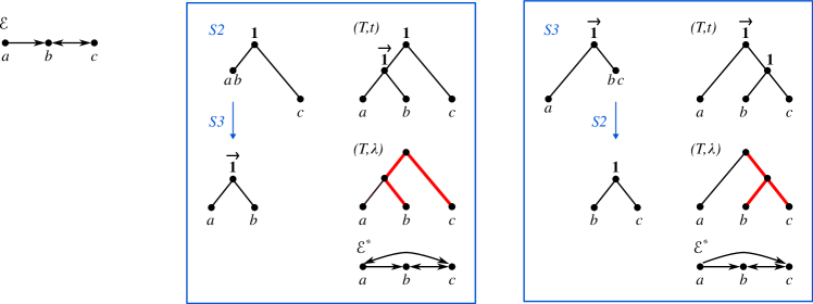
The proof of Thm. 3.2 provides a recipe to construct a Fitch-cotree $(T,t)$ explaining a tuple $\mathcal{E}$. We observe, furthermore, that two or even all three alternatives (S1), (S2.a), and (S3.a) may be satisfied simultaneously, see Fig. 2 for an illustrative example. In this case, it becomes necessary to check stepwisely whether conditions (S2.b) and/or (S3.b) holds. Potentially, this result in exponential effort to determine recursively whether $\mathcal{E}[C]$ or $\mathcal{E}[V\setminus C]$ is Fitch-sat. The following simple lemma shows, however, that the alternatives always yield consistent results:

Lemma 4

Let $\mathcal{E}=(E_{0},E_{1},E_{\overrightarrow{1}})$ be a partial tuple on $V$. Then

  • (S1) and (S2.a) implies (S2.b);

  • (S1) and (S3.a) implies (S3.b);

  • (S2a) and (S3a) implies that (S2.b) and (S3.b) are equivalent.

Proof

If (S1) holds, then Thm. 3.2 implies that $\mathcal{E}$ is Fitch-sat. If (S2.a) holds, then heredity (Lemma 2) implies that $\mathcal{E}[C]$ is Fitch-sat and thus (S2.b) is satisfied. Analogously, if (S3.a) holds, then $\mathcal{E}[V\setminus C]$ is Fitch-sat and thus (S3.b) holds. Now suppose (S2a) and (S3a) are satisfied but (S1) does not hold. Then $\mathcal{E}$ is Fitch-sat if and only if one of (S2.b) or (S3.b) holds; in the affirmative case, heredity again implies that both (S2.b) and (S3.b) are satisfied. ∎

It follows that testing whether $\mathcal{E}$ can be achieved by checking if any one of the three conditions (S1), (S2), or (S3) holds and, if necessary, recursing down on $\mathcal{E}[C]$ or $\mathcal{E}[V\setminus C]$. This give rise to Alg. 1.

Algorithm 1 Recognition of Fitch-sat partial tuple $\mathcal{E}$ on $V$ and reconstruction of a cotree $(T,t)$ that explains $\mathcal{E}$.
1: Partial tuples $\mathcal{E}=(E_{0},E_{1},E_{\overrightarrow{1}})$
2: A cotree $(T,t)$ that explains $\mathcal{E}$, if one exists or the statement “$\mathcal{E}$ is not Fitch-satisfiable”
3: Call BuildFitchCotree($V,\mathcal{E}$)
4: Call BuildFitchCotree($V,\mathcal{E}$) Call BuildFitchCotree($V,\mathcal{E}$) function BuildFitchCotree($V,\mathcal{E}=(E_{0},E_{1},E_{\overrightarrow{1}})$) $\triangleright$ $G_{0}$, $G_{1}$ and $G_{\overrightarrow{1}}$ are defined as in Thm. 3.2 for given $\mathcal{E}$ Call BuildFitchCotree($V,\mathcal{E}$) Call BuildFitchCotree($V,\mathcal{E}$) function BuildFitchCotree($V,\mathcal{E}=(E_{0},E_{1},E_{\overrightarrow{1}})$) $\triangleright$ $G_{0}$, $G_{1}$ and $G_{\overrightarrow{1}}$ are defined as in Thm. 3.2 for given $\mathcal{E}$
5:      Call BuildFitchCotree($V,\mathcal{E}$) Call BuildFitchCotree($V,\mathcal{E}$) function BuildFitchCotree($V,\mathcal{E}=(E_{0},E_{1},E_{\overrightarrow{1}})$) $\triangleright$ $G_{0}$, $G_{1}$ and $G_{\overrightarrow{1}}$ are defined as in Thm. 3.2 for given $\mathcal{E}$ Call BuildFitchCotree($V,\mathcal{E}$) Call BuildFitchCotree($V,\mathcal{E}$) function BuildFitchCotree($V,\mathcal{E}=(E_{0},E_{1},E_{\overrightarrow{1}})$) $\triangleright$ $G_{0}$, $G_{1}$ and $G_{\overrightarrow{1}}$ are defined as in Thm. 3.2 for given $\mathcal{E}$ Call BuildFitchCotree($V,\mathcal{E}$) Call BuildFitchCotree($V,\mathcal{E}$) function BuildFitchCotree($V,\mathcal{E}=(E_{0},E_{1},E_{\overrightarrow{1}})$) $\triangleright$ $G_{0}$, $G_{1}$ and $G_{\overrightarrow{1}}$ are defined as in Thm. 3.2 for given $\mathcal{E}$ if $|V|=1$ then return the cotree $((V,\emptyset),\emptyset)$ Call BuildFitchCotree($V,\mathcal{E}$) Call BuildFitchCotree($V,\mathcal{E}$) function BuildFitchCotree($V,\mathcal{E}=(E_{0},E_{1},E_{\overrightarrow{1}})$) $\triangleright$ $G_{0}$, $G_{1}$ and $G_{\overrightarrow{1}}$ are defined as in Thm. 3.2 for given $\mathcal{E}$ Call BuildFitchCotree($V,\mathcal{E}$) Call BuildFitchCotree($V,\mathcal{E}$) function BuildFitchCotree($V,\mathcal{E}=(E_{0},E_{1},E_{\overrightarrow{1}})$) $\triangleright$ $G_{0}$, $G_{1}$ and $G_{\overrightarrow{1}}$ are defined as in Thm. 3.2 for given $\mathcal{E}$ if $|V|=1$ then return the cotree $((V,\emptyset),\emptyset)$
6:      Call BuildFitchCotree($V,\mathcal{E}$) Call BuildFitchCotree($V,\mathcal{E}$) function BuildFitchCotree($V,\mathcal{E}=(E_{0},E_{1},E_{\overrightarrow{1}})$) $\triangleright$ $G_{0}$, $G_{1}$ and $G_{\overrightarrow{1}}$ are defined as in Thm. 3.2 for given $\mathcal{E}$ Call BuildFitchCotree($V,\mathcal{E}$) Call BuildFitchCotree($V,\mathcal{E}$) function BuildFitchCotree($V,\mathcal{E}=(E_{0},E_{1},E_{\overrightarrow{1}})$) $\triangleright$ $G_{0}$, $G_{1}$ and $G_{\overrightarrow{1}}$ are defined as in Thm. 3.2 for given $\mathcal{E}$ if $|V|=1$ then return the cotree $((V,\emptyset),\emptyset)$ Call BuildFitchCotree($V,\mathcal{E}$) Call BuildFitchCotree($V,\mathcal{E}$) function BuildFitchCotree($V,\mathcal{E}=(E_{0},E_{1},E_{\overrightarrow{1}})$) $\triangleright$ $G_{0}$, $G_{1}$ and $G_{\overrightarrow{1}}$ are defined as in Thm. 3.2 for given $\mathcal{E}$ Call BuildFitchCotree($V,\mathcal{E}$) Call BuildFitchCotree($V,\mathcal{E}$) function BuildFitchCotree($V,\mathcal{E}=(E_{0},E_{1},E_{\overrightarrow{1}})$) $\triangleright$ $G_{0}$, $G_{1}$ and $G_{\overrightarrow{1}}$ are defined as in Thm. 3.2 for given $\mathcal{E}$ if $|V|=1$ then return the cotree $((V,\emptyset),\emptyset)$ Call BuildFitchCotree($V,\mathcal{E}$) Call BuildFitchCotree($V,\mathcal{E}$) function BuildFitchCotree($V,\mathcal{E}=(E_{0},E_{1},E_{\overrightarrow{1}})$) $\triangleright$ $G_{0}$, $G_{1}$ and $G_{\overrightarrow{1}}$ are defined as in Thm. 3.2 for given $\mathcal{E}$ Call BuildFitchCotree($V,\mathcal{E}$) Call BuildFitchCotree($V,\mathcal{E}$) function BuildFitchCotree($V,\mathcal{E}=(E_{0},E_{1},E_{\overrightarrow{1}})$) $\triangleright$ $G_{0}$, $G_{1}$ and $G_{\overrightarrow{1}}$ are defined as in Thm. 3.2 for given $\mathcal{E}$ if $|V|=1$ then return the cotree $((V,\emptyset),\emptyset)$ Call BuildFitchCotree($V,\mathcal{E}$) Call BuildFitchCotree($V,\mathcal{E}$) function BuildFitchCotree($V,\mathcal{E}=(E_{0},E_{1},E_{\overrightarrow{1}})$) $\triangleright$ $G_{0}$, $G_{1}$ and $G_{\overrightarrow{1}}$ are defined as in Thm. 3.2 for given $\mathcal{E}$ Call BuildFitchCotree($V,\mathcal{E}$) Call BuildFitchCotree($V,\mathcal{E}$) function BuildFitchCotree($V,\mathcal{E}=(E_{0},E_{1},E_{\overrightarrow{1}})$) $\triangleright$ $G_{0}$, $G_{1}$ and $G_{\overrightarrow{1}}$ are defined as in Thm. 3.2 for given $\mathcal{E}$ if $|V|=1$ then return the cotree $((V,\emptyset),\emptyset)$ else if $G_{0}$ is edge-less (otherwise if $G_{1}$ is disconnected) then $\triangleright$ check (S1) (resp., (S2)) Call BuildFitchCotree($V,\mathcal{E}$) Call BuildFitchCotree($V,\mathcal{E}$) function BuildFitchCotree($V,\mathcal{E}=(E_{0},E_{1},E_{\overrightarrow{1}})$) $\triangleright$ $G_{0}$, $G_{1}$ and $G_{\overrightarrow{1}}$ are defined as in Thm. 3.2 for given $\mathcal{E}$ Call BuildFitchCotree($V,\mathcal{E}$) Call BuildFitchCotree($V,\mathcal{E}$) function BuildFitchCotree($V,\mathcal{E}=(E_{0},E_{1},E_{\overrightarrow{1}})$) $\triangleright$ $G_{0}$, $G_{1}$ and $G_{\overrightarrow{1}}$ are defined as in Thm. 3.2 for given $\mathcal{E}$ if $|V|=1$ then return the cotree $((V,\emptyset),\emptyset)$ Call BuildFitchCotree($V,\mathcal{E}$) Call BuildFitchCotree($V,\mathcal{E}$) function BuildFitchCotree($V,\mathcal{E}=(E_{0},E_{1},E_{\overrightarrow{1}})$) $\triangleright$ $G_{0}$, $G_{1}$ and $G_{\overrightarrow{1}}$ are defined as in Thm. 3.2 for given $\mathcal{E}$ Call BuildFitchCotree($V,\mathcal{E}$) Call BuildFitchCotree($V,\mathcal{E}$) function BuildFitchCotree($V,\mathcal{E}=(E_{0},E_{1},E_{\overrightarrow{1}})$) $\triangleright$ $G_{0}$, $G_{1}$ and $G_{\overrightarrow{1}}$ are defined as in Thm. 3.2 for given $\mathcal{E}$ if $|V|=1$ then return the cotree $((V,\emptyset),\emptyset)$ Call BuildFitchCotree($V,\mathcal{E}$) Call BuildFitchCotree($V,\mathcal{E}$) function BuildFitchCotree($V,\mathcal{E}=(E_{0},E_{1},E_{\overrightarrow{1}})$) $\triangleright$ $G_{0}$, $G_{1}$ and $G_{\overrightarrow{1}}$ are defined as in Thm. 3.2 for given $\mathcal{E}$ Call BuildFitchCotree($V,\mathcal{E}$) Call BuildFitchCotree($V,\mathcal{E}$) function BuildFitchCotree($V,\mathcal{E}=(E_{0},E_{1},E_{\overrightarrow{1}})$) $\triangleright$ $G_{0}$, $G_{1}$ and $G_{\overrightarrow{1}}$ are defined as in Thm. 3.2 for given $\mathcal{E}$ if $|V|=1$ then return the cotree $((V,\emptyset),\emptyset)$ else if $G_{0}$ is edge-less (otherwise if $G_{1}$ is disconnected) then $\triangleright$ check (S1) (resp., (S2))
7:          Call BuildFitchCotree($V,\mathcal{E}$) Call BuildFitchCotree($V,\mathcal{E}$) function BuildFitchCotree($V,\mathcal{E}=(E_{0},E_{1},E_{\overrightarrow{1}})$) $\triangleright$ $G_{0}$, $G_{1}$ and $G_{\overrightarrow{1}}$ are defined as in Thm. 3.2 for given $\mathcal{E}$ Call BuildFitchCotree($V,\mathcal{E}$) Call BuildFitchCotree($V,\mathcal{E}$) function BuildFitchCotree($V,\mathcal{E}=(E_{0},E_{1},E_{\overrightarrow{1}})$) $\triangleright$ $G_{0}$, $G_{1}$ and $G_{\overrightarrow{1}}$ are defined as in Thm. 3.2 for given $\mathcal{E}$ if $|V|=1$ then return the cotree $((V,\emptyset),\emptyset)$ Call BuildFitchCotree($V,\mathcal{E}$) Call BuildFitchCotree($V,\mathcal{E}$) function BuildFitchCotree($V,\mathcal{E}=(E_{0},E_{1},E_{\overrightarrow{1}})$) $\triangleright$ $G_{0}$, $G_{1}$ and $G_{\overrightarrow{1}}$ are defined as in Thm. 3.2 for given $\mathcal{E}$ Call BuildFitchCotree($V,\mathcal{E}$) Call BuildFitchCotree($V,\mathcal{E}$) function BuildFitchCotree($V,\mathcal{E}=(E_{0},E_{1},E_{\overrightarrow{1}})$) $\triangleright$ $G_{0}$, $G_{1}$ and $G_{\overrightarrow{1}}$ are defined as in Thm. 3.2 for given $\mathcal{E}$ if $|V|=1$ then return the cotree $((V,\emptyset),\emptyset)$ Call BuildFitchCotree($V,\mathcal{E}$) Call BuildFitchCotree($V,\mathcal{E}$) function BuildFitchCotree($V,\mathcal{E}=(E_{0},E_{1},E_{\overrightarrow{1}})$) $\triangleright$ $G_{0}$, $G_{1}$ and $G_{\overrightarrow{1}}$ are defined as in Thm. 3.2 for given $\mathcal{E}$ Call BuildFitchCotree($V,\mathcal{E}$) Call BuildFitchCotree($V,\mathcal{E}$) function BuildFitchCotree($V,\mathcal{E}=(E_{0},E_{1},E_{\overrightarrow{1}})$) $\triangleright$ $G_{0}$, $G_{1}$ and $G_{\overrightarrow{1}}$ are defined as in Thm. 3.2 for given $\mathcal{E}$ if $|V|=1$ then return the cotree $((V,\emptyset),\emptyset)$ else if $G_{0}$ is edge-less (otherwise if $G_{1}$ is disconnected) then $\triangleright$ check (S1) (resp., (S2)) $\mathcal{C}\coloneqq$ the set of connected components $\{C_{1},\dots,C_{k}\}$ of $G_{0}$ (resp. $G_{1}$) $\mathcal{C}\coloneqq$ the set of connected components $\{C_{1},\dots,C_{k}\}$ of $G_{0}$ (resp. $G_{1}$)
8:          $\mathcal{C}\coloneqq$ the set of connected components $\{C_{1},\dots,C_{k}\}$ of $G_{0}$ (resp. $G_{1}$) $\mathcal{T}\coloneqq$ set $\{\textsc{BuildFitchCotree}(C_{i},\ \mathcal{E}[C_{i}])\mid C_{i}\in\mathcal{C}\}$ $\mathcal{T}\coloneqq$ set $\{\textsc{BuildFitchCotree}(C_{i},\ \mathcal{E}[C_{i}])\mid C_{i}\in\mathcal{C}\}$
9:          $\mathcal{T}\coloneqq$ set $\{\textsc{BuildFitchCotree}(C_{i},\ \mathcal{E}[C_{i}])\mid C_{i}\in\mathcal{C}\}$ return the cotree from joining the cotrees in $\mathcal{T}$ under a new root labeled 00 (resp. $1$) return the cotree from joining the cotrees in $\mathcal{T}$ under a new root labeled 00 (resp. $1$)
10:      return the cotree from joining the cotrees in $\mathcal{T}$ under a new root labeled 00 (resp. $1$) return the cotree from joining the cotrees in $\mathcal{T}$ under a new root labeled 00 (resp. $1$) return the cotree from joining the cotrees in $\mathcal{T}$ under a new root labeled 00 (resp. $1$) return the cotree from joining the cotrees in $\mathcal{T}$ under a new root labeled 00 (resp. $1$) else if $G_{\overrightarrow{1}}$ has more than one strongly connected component then $\triangleright$ check (S3) return the cotree from joining the cotrees in $\mathcal{T}$ under a new root labeled 00 (resp. $1$) return the cotree from joining the cotrees in $\mathcal{T}$ under a new root labeled 00 (resp. $1$) return the cotree from joining the cotrees in $\mathcal{T}$ under a new root labeled 00 (resp. $1$) else if $G_{\overrightarrow{1}}$ has more than one strongly connected component then $\triangleright$ check (S3)
11:          return the cotree from joining the cotrees in $\mathcal{T}$ under a new root labeled 00 (resp. $1$) return the cotree from joining the cotrees in $\mathcal{T}$ under a new root labeled 00 (resp. $1$) return the cotree from joining the cotrees in $\mathcal{T}$ under a new root labeled 00 (resp. $1$) else if $G_{\overrightarrow{1}}$ has more than one strongly connected component then $\triangleright$ check (S3) $\mathcal{C}\coloneqq$ the set of strongly connected components $\{C_{1},\dots,C_{k}\}$ of $G_{\overrightarrow{1}}$ $\mathcal{C}\coloneqq$ the set of strongly connected components $\{C_{1},\dots,C_{k}\}$ of $G_{\overrightarrow{1}}$
12:          $\mathcal{C}\coloneqq$ the set of strongly connected components $\{C_{1},\dots,C_{k}\}$ of $G_{\overrightarrow{1}}$ $I\leftarrow\emptyset$ $I\leftarrow\emptyset$
13:          $I\leftarrow\emptyset$ $I\leftarrow\emptyset$ $I\leftarrow\emptyset$ for all $i\in\{1,\dots,k\}$ do $I\leftarrow\emptyset$ $I\leftarrow\emptyset$ for all $i\in\{1,\dots,k\}$ do
14:               $I\leftarrow\emptyset$ $I\leftarrow\emptyset$ for all $i\in\{1,\dots,k\}$ do $I\leftarrow\emptyset$ $I\leftarrow\emptyset$ for all $i\in\{1,\dots,k\}$ do $I\leftarrow\emptyset$ $I\leftarrow\emptyset$ for all $i\in\{1,\dots,k\}$ do if $G_{0}[C_{i}]$ is edge-less then $I\leftarrow I\cup\{i\}$ $I\leftarrow\emptyset$ $I\leftarrow\emptyset$ for all $i\in\{1,\dots,k\}$ do $I\leftarrow\emptyset$ $I\leftarrow\emptyset$ for all $i\in\{1,\dots,k\}$ do if $G_{0}[C_{i}]$ is edge-less then $I\leftarrow I\cup\{i\}$ $I\leftarrow\emptyset$ $I\leftarrow\emptyset$ for all $i\in\{1,\dots,k\}$ do $I\leftarrow\emptyset$ $I\leftarrow\emptyset$ for all $i\in\{1,\dots,k\}$ do if $G_{0}[C_{i}]$ is edge-less then $I\leftarrow I\cup\{i\}$                         
15:          $I\leftarrow\emptyset$ $I\leftarrow\emptyset$ for all $i\in\{1,\dots,k\}$ do $I\leftarrow\emptyset$ $I\leftarrow\emptyset$ for all $i\in\{1,\dots,k\}$ do if $G_{0}[C_{i}]$ is edge-less then $I\leftarrow I\cup\{i\}$ $I\leftarrow\emptyset$ $I\leftarrow\emptyset$ for all $i\in\{1,\dots,k\}$ do $I\leftarrow\emptyset$ $I\leftarrow\emptyset$ for all $i\in\{1,\dots,k\}$ do if $G_{0}[C_{i}]$ is edge-less then $I\leftarrow I\cup\{i\}$ $I\leftarrow\emptyset$ $I\leftarrow\emptyset$ for all $i\in\{1,\dots,k\}$ do $I\leftarrow\emptyset$ $I\leftarrow\emptyset$ for all $i\in\{1,\dots,k\}$ do if $G_{0}[C_{i}]$ is edge-less then $I\leftarrow I\cup\{i\}$ if $I=\emptyset$ then $I\leftarrow\emptyset$ $I\leftarrow\emptyset$ for all $i\in\{1,\dots,k\}$ do $I\leftarrow\emptyset$ $I\leftarrow\emptyset$ for all $i\in\{1,\dots,k\}$ do if $G_{0}[C_{i}]$ is edge-less then $I\leftarrow I\cup\{i\}$ $I\leftarrow\emptyset$ $I\leftarrow\emptyset$ for all $i\in\{1,\dots,k\}$ do $I\leftarrow\emptyset$ $I\leftarrow\emptyset$ for all $i\in\{1,\dots,k\}$ do if $G_{0}[C_{i}]$ is edge-less then $I\leftarrow I\cup\{i\}$ if $I=\emptyset$ then
16:               $I\leftarrow\emptyset$ $I\leftarrow\emptyset$ for all $i\in\{1,\dots,k\}$ do $I\leftarrow\emptyset$ $I\leftarrow\emptyset$ for all $i\in\{1,\dots,k\}$ do if $G_{0}[C_{i}]$ is edge-less then $I\leftarrow I\cup\{i\}$ $I\leftarrow\emptyset$ $I\leftarrow\emptyset$ for all $i\in\{1,\dots,k\}$ do $I\leftarrow\emptyset$ $I\leftarrow\emptyset$ for all $i\in\{1,\dots,k\}$ do if $G_{0}[C_{i}]$ is edge-less then $I\leftarrow I\cup\{i\}$ if $I=\emptyset$ then Halt and output: “$\mathcal{E}$ is not Fitch-satisfiable” $\triangleright$ (S3.a.II.i) not satisfied Halt and output: “$\mathcal{E}$ is not Fitch-satisfiable” $\triangleright$ (S3.a.II.i) not satisfied
17:          Halt and output: “$\mathcal{E}$ is not Fitch-satisfiable” $\triangleright$ (S3.a.II.i) not satisfied Halt and output: “$\mathcal{E}$ is not Fitch-satisfiable” $\triangleright$ (S3.a.II.i) not satisfied Halt and output: “$\mathcal{E}$ is not Fitch-satisfiable” $\triangleright$ (S3.a.II.i) not satisfied Halt and output: “$\mathcal{E}$ is not Fitch-satisfiable” $\triangleright$ (S3.a.II.i) not satisfied else if there is no topological order $\ll$ of $G_{\overrightarrow{1}}/\{C_{1},\dots,C_{k}\}$ with $\ll$-minimal element $C_{i}$ with $i\in I$ then Halt and output: “$\mathcal{E}$ is not Fitch-satisfiable” $\triangleright$ (S3.a.II.i) not satisfied Halt and output: “$\mathcal{E}$ is not Fitch-satisfiable” $\triangleright$ (S3.a.II.i) not satisfied Halt and output: “$\mathcal{E}$ is not Fitch-satisfiable” $\triangleright$ (S3.a.II.i) not satisfied else if there is no topological order $\ll$ of $G_{\overrightarrow{1}}/\{C_{1},\dots,C_{k}\}$ with $\ll$-minimal element $C_{i}$ with $i\in I$ then
18:               Halt and output: “$\mathcal{E}$ is not Fitch-satisfiable” $\triangleright$ (S3.a.II.i) not satisfied Halt and output: “$\mathcal{E}$ is not Fitch-satisfiable” $\triangleright$ (S3.a.II.i) not satisfied Halt and output: “$\mathcal{E}$ is not Fitch-satisfiable” $\triangleright$ (S3.a.II.i) not satisfied else if there is no topological order $\ll$ of $G_{\overrightarrow{1}}/\{C_{1},\dots,C_{k}\}$ with $\ll$-minimal element $C_{i}$ with $i\in I$ then Halt and output: “$\mathcal{E}$ is not Fitch-satisfiable” $\triangleright$ (S3.a.II.ii) not satisfied Halt and output: “$\mathcal{E}$ is not Fitch-satisfiable” $\triangleright$ (S3.a.II.ii) not satisfied
19:          Halt and output: “$\mathcal{E}$ is not Fitch-satisfiable” $\triangleright$ (S3.a.II.ii) not satisfied Halt and output: “$\mathcal{E}$ is not Fitch-satisfiable” $\triangleright$ (S3.a.II.ii) not satisfied Halt and output: “$\mathcal{E}$ is not Fitch-satisfiable” $\triangleright$ (S3.a.II.ii) not satisfied Halt and output: “$\mathcal{E}$ is not Fitch-satisfiable” $\triangleright$ (S3.a.II.ii) not satisfied else Halt and output: “$\mathcal{E}$ is not Fitch-satisfiable” $\triangleright$ (S3.a.II.ii) not satisfied Halt and output: “$\mathcal{E}$ is not Fitch-satisfiable” $\triangleright$ (S3.a.II.ii) not satisfied Halt and output: “$\mathcal{E}$ is not Fitch-satisfiable” $\triangleright$ (S3.a.II.ii) not satisfied else
20:               Halt and output: “$\mathcal{E}$ is not Fitch-satisfiable” $\triangleright$ (S3.a.II.ii) not satisfied Halt and output: “$\mathcal{E}$ is not Fitch-satisfiable” $\triangleright$ (S3.a.II.ii) not satisfied Halt and output: “$\mathcal{E}$ is not Fitch-satisfiable” $\triangleright$ (S3.a.II.ii) not satisfied else $\ll\coloneqq$ a topol. order on the quotient $G_{\overrightarrow{1}}/\{C_{1},\dots,C_{k}\}$ with $\ll$-minimal element $C^{*}\coloneqq C_{i}$ for some $i\in I$ $\ll\coloneqq$ a topol. order on the quotient $G_{\overrightarrow{1}}/\{C_{1},\dots,C_{k}\}$ with $\ll$-minimal element $C^{*}\coloneqq C_{i}$ for some $i\in I$
21:               $\ll\coloneqq$ a topol. order on the quotient $G_{\overrightarrow{1}}/\{C_{1},\dots,C_{k}\}$ with $\ll$-minimal element $C^{*}\coloneqq C_{i}$ for some $i\in I$ $\mathcal{T}\coloneqq\{\textsc{BuildFitchCotree}(C,\ \mathcal{E}[C])\mid C\in\{C^{*},V\setminus C^{*}\}$ $\mathcal{T}\coloneqq\{\textsc{BuildFitchCotree}(C,\ \mathcal{E}[C])\mid C\in\{C^{*},V\setminus C^{*}\}$
22:               $\mathcal{T}\coloneqq\{\textsc{BuildFitchCotree}(C,\ \mathcal{E}[C])\mid C\in\{C^{*},V\setminus C^{*}\}$ return the cotree $(T,t)$ obtained by joining the cotrees in $\mathcal{T}$ under a new root with label $\overrightarrow{1}$,             where the tree $(T^{*},t^{*})$ that explains $C^{*}$ is placed left of the tree $(\widehat{T},\widehat{t})$ that explains $V\setminus C$ return the cotree $(T,t)$ obtained by joining the cotrees in $\mathcal{T}$ under a new root with label $\overrightarrow{1}$,             where the tree $(T^{*},t^{*})$ that explains $C^{*}$ is placed left of the tree $(\widehat{T},\widehat{t})$ that explains $V\setminus C$ return the cotree $(T,t)$ obtained by joining the cotrees in $\mathcal{T}$ under a new root with label $\overrightarrow{1}$,             where the tree $(T^{*},t^{*})$ that explains $C^{*}$ is placed left of the tree $(\widehat{T},\widehat{t})$ that explains $V\setminus C$          
23:      return the cotree $(T,t)$ obtained by joining the cotrees in $\mathcal{T}$ under a new root with label $\overrightarrow{1}$,             where the tree $(T^{*},t^{*})$ that explains $C^{*}$ is placed left of the tree $(\widehat{T},\widehat{t})$ that explains $V\setminus C$ return the cotree $(T,t)$ obtained by joining the cotrees in $\mathcal{T}$ under a new root with label $\overrightarrow{1}$,             where the tree $(T^{*},t^{*})$ that explains $C^{*}$ is placed left of the tree $(\widehat{T},\widehat{t})$ that explains $V\setminus C$ return the cotree $(T,t)$ obtained by joining the cotrees in $\mathcal{T}$ under a new root with label $\overrightarrow{1}$,             where the tree $(T^{*},t^{*})$ that explains $C^{*}$ is placed left of the tree $(\widehat{T},\widehat{t})$ that explains $V\setminus C$ return the cotree $(T,t)$ obtained by joining the cotrees in $\mathcal{T}$ under a new root with label $\overrightarrow{1}$,             where the tree $(T^{*},t^{*})$ that explains $C^{*}$ is placed left of the tree $(\widehat{T},\widehat{t})$ that explains $V\setminus C$ else return the cotree $(T,t)$ obtained by joining the cotrees in $\mathcal{T}$ under a new root with label $\overrightarrow{1}$,             where the tree $(T^{*},t^{*})$ that explains $C^{*}$ is placed left of the tree $(\widehat{T},\widehat{t})$ that explains $V\setminus C$ return the cotree $(T,t)$ obtained by joining the cotrees in $\mathcal{T}$ under a new root with label $\overrightarrow{1}$,             where the tree $(T^{*},t^{*})$ that explains $C^{*}$ is placed left of the tree $(\widehat{T},\widehat{t})$ that explains $V\setminus C$ return the cotree $(T,t)$ obtained by joining the cotrees in $\mathcal{T}$ under a new root with label $\overrightarrow{1}$,             where the tree $(T^{*},t^{*})$ that explains $C^{*}$ is placed left of the tree $(\widehat{T},\widehat{t})$ that explains $V\setminus C$ else
24:          return the cotree $(T,t)$ obtained by joining the cotrees in $\mathcal{T}$ under a new root with label $\overrightarrow{1}$,             where the tree $(T^{*},t^{*})$ that explains $C^{*}$ is placed left of the tree $(\widehat{T},\widehat{t})$ that explains $V\setminus C$ return the cotree $(T,t)$ obtained by joining the cotrees in $\mathcal{T}$ under a new root with label $\overrightarrow{1}$,             where the tree $(T^{*},t^{*})$ that explains $C^{*}$ is placed left of the tree $(\widehat{T},\widehat{t})$ that explains $V\setminus C$ return the cotree $(T,t)$ obtained by joining the cotrees in $\mathcal{T}$ under a new root with label $\overrightarrow{1}$,             where the tree $(T^{*},t^{*})$ that explains $C^{*}$ is placed left of the tree $(\widehat{T},\widehat{t})$ that explains $V\setminus C$ else Halt and output: “$\mathcal{E}$ is not Fitch-satisfiable” Halt and output: “$\mathcal{E}$ is not Fitch-satisfiable” Halt and output: “$\mathcal{E}$ is not Fitch-satisfiable”      
Refer to caption
Figure 2: A partial tuple $\mathcal{E}=(E_{0},E_{1},E_{\overrightarrow{1}})$ on $V=\{a,b,c\}$ with $E_{0}=\emptyset$, $E_{1}=\{(b,c),(c,b)\}$ (bi-directional arc), and $E_{\overrightarrow{1}}=\{(a,b)\}$ (single arc) is shown on the left. Observe that (S1) is not satisfied while (S2.a) and (S3.a) hold for $\mathcal{E}$. Application of the different rules and subsequent construction of the Fitch-cotrees that explain the subgraphs induced by the respective (strongly) connected components results in two Fitch-cotrees that both explain $\mathcal{E}$. Hence, we obtain two different edge-labeled Fitch-trees $(T,\lambda)$ (with HGT-edges drawn in bold-red) that both explain $\mathcal{E}$.
Lemma 5

Let $\mathcal{E}=(E_{0},E_{1},E_{\overrightarrow{1}})$ be a partial tuple. Then Alg. 1 either outputs a Fitch-cotree $(T,t)$ that explains $\mathcal{E}$ or recognizes that $\mathcal{E}$ is not Fitch-sat.

Proof

Let $\mathcal{E}=(E_{0},E_{1},E_{\overrightarrow{1}})$ be a partial tuple on $V$ that serves as input for Alg. 1. In Alg. 1, the function BuildFitchCotree is called and the algorithm we will try and build a Fitch-cotree explaining a full Fitch-sat tuple that extends $\mathcal{E}$. By Lemma 4, the order in which (S1), (S2), and (S3) is tested is arbitrary. If $|V|=1$, then $\mathcal{E}$ is already full and Fitch-sat, and $(T,t)=((V,\emptyset);\emptyset)$ is a valid Fitch-cotree explaining $\mathcal{E}$, and thus returned on Line 7. If none of the conditions (S1), (S2), or (S3) is satisfied, Thm. 3.2 implies that $\mathcal{E}$ is not Fitch-sat, and Alg. 1 correctly returns “$\mathcal{E}$ is not Fitch-sat”.

If Rule (S1) or (S2.a), resp., is satisfied (Line 7), then Alg. 1 is called recursively on each of the connected components defined by $G_{0}$ or $G_{1}$, respectively. In case of (S1), the connected components are all single vertices and we obtain a star-tree $(T,t)$ whose root is labeled “0” as outlined in the proof of the if direction of Thm. 3.2. Since $(T,t)$ is a Fitch-cotree that explains $\mathcal{E}$, it follows that $\mathcal{E}$ is Fitch-sat. In case of (S2.a), condition (S2.b) must be tested. If each of the connected components are indeed Fitch-sat, the obtained Fitch-cotrees are joined into a single cotree $(T,t)$ that explains a full tuple $\mathcal{E}^{*}$ which extends $\mathcal{E}$. In particular, since no constraints are imposed on the root $\rho_{T}$, which has label “1”, $(T,t)$ is a Fitch-cotree. Consequently, $\mathcal{E}$ is Fitch-sat and explained by $(T,t)$.

Suppose, finally, that $\mathcal{E}$ satisfies (S3.a) and let $\mathcal{C}\coloneqq\{C_{1},\dots,C_{k}\}$ be the the set of strongly connected components of $G_{\overrightarrow{1}}$. Since (S3.a.II) is satisfied, there must be a $C_{i}\in\mathcal{C}$ for which $G[C_{i}]$ is edge-less, i.e., the set $I$ as computed in Line 16 cannot be empty. In particular, there is a topological order $\ll$ of $G_{\overrightarrow{1}}/\{C_{1},\dots,C_{k}\}$ with $\ll$-minimal element $C^{*}\coloneqq C_{i}$ for some $i\in I$. It is now checked, if $\mathcal{E}[C^{*}]$ and $\mathcal{E}[\widehat{C}]$ are Fitch-sat, where $\widehat{C}\coloneqq V\setminus C$. If this is the case, two Fitch-cotrees $(T^{*},t^{*})$ and $(\widehat{T},\widehat{t})$ that explain $\mathcal{E}[C^{*}]$ and $\mathcal{E}[\widehat{C}]$ are returned. We then join these cotrees in under a new root with label $\overrightarrow{1}$, where the tree $(T^{*},t^{*})$ is placed left from $(\widehat{T},\widehat{t})$. The latter results in a cotree $(T,t)$ that explains $\mathcal{E}$. It remains to show that $(T,t)$ is a Fitch-cotree. Since, $\rho_{T}$ has precisely two children $\rho_{T^{*}}$ and $\rho_{\widehat{T}}$ and $\rho_{T^{*}}$ is left from $\rho_{\widehat{T}}$, we must show that that the tree $(T^{*},t^{*})$ computed in the recursive calls does not contain an inner vertex $v$ with label $t(v)\neq 1$. The recursive call with $\mathcal{E}[C^{*}]$ first checks if $|C^{*}|=1$ (line 7) and the continues with checking if $G_{0}[C^{*}]$ is edge-less (7). Since $G_{0}[C^{*}]$ is edge-less, at least one of the steps are satisfied and either the single-vertex tree or a star tree whose root has label “0” with be returned. Consequently, $(T^{*},t^{*})$ does not contain an inner vertex $v$ with label $t(v)\neq 1$ and thus, $(T,t)$ is a Fitch-cotree that explains $\mathcal{E}$. Hence, $\mathcal{E}$ is Fitch-sat. ∎

Theorem 4.1

Let $\mathcal{E}=(E_{0},E_{1},E_{\overrightarrow{1}})$ be a partial tuple, $n=|V|$ and $m=|E_{0}\cup E_{1}\cup E_{\overrightarrow{1}}|$. Then, Alg. 1 computes a Fitch-cotree $(T,t)$ that explains $\mathcal{E}$ or identifies that $\mathcal{E}$ is not Fitch-sat in $O(n^{2}+nm)$ time.

Proof

Correctness is established in Lemma 5. We first note that in each single call of BuildFitchCotree, all necessary di-graphs defined in (S1), (S2) and (S3) can be computed in $O(n+m)$ time. Furthermore, each of the following tasks can be performed in $O(n+m)$ time: finding the (strongly) connected components of each digraph, construction of the quotient graphs, and finding the topological order on the quotient graph using Kahn’s algorithm [10]. Moreover, the vertex end edge sets $V[C]$ and $\mathcal{E}[C]$ for the (strongly) connected components $C$ (or their unions) can constructed in $O(n+m)$ time by going through every element in $V$ and $\mathcal{E}$ and assigning each pair to their respective induced subset. Thus, every pass of BuildFitchCotree takes $O(n+m)$ time. Since every call of BuildFitchCotree either halts or adds a vertex to the final constructed Fitch-cotree, and the number of vertices in this tree is bounded by the number $n$ of leaves, it follows that BuildFitchCotree is called at most $O(n)$ times resulting in an overall running time $O(n(n+m))$. ∎

Instead of asking only for the existence of a Fitch-completion of a tuple $\mathcal{E}=(E_{0},E_{1},E_{\overrightarrow{1}})$, it is of interest to ask for the completion that maximizes a total score for the the pairs of distinct vertices $x,y$ that are not already classified by $\mathcal{E}$, i.e., $\{x,y\}\in\overline{\mathcal{E}}\coloneqq\{\{x,y\}\notin(E_{0}\cup E_{1}\cup E_{\overrightarrow{1}})^{sym}\}$. For every pair of vertices there are four possibilities $x\mathop{::}y\in\{x\rightleftharpoons y,x\to y,x\leftarrow y,x\mathop{\text{\textvisiblespace}}y\}$. The score $w(x\mathop{::}y)$ may be a log-odds ratio for observing one of the four possible xenology relationship as determined from experimental data. Let us write $F=F_{\mathcal{E}^{*}}$ for the Fitch graph defined by the extension $\mathcal{E}^{*}$ of $\mathcal{E}$ and associate with it the the total weight of relations added, i.e.,

$$f(F)=\sum_{\{x,y\}\in\overline{\mathcal{E}}}w(F[\{x,y\}])$$ (1)

The weighted Fitch-graph completion problem can also be seen as special case of the problem with empty tuple $\mathcal{E}^{\emptyset}\coloneqq(\emptyset,\emptyset,\emptyset)$. To see this, suppose first that an arbitrary partial input tuple $\mathcal{E}$ is given. For each two vertices $x,y$ for which $\{x,y\}\notin\overline{\mathcal{E}}$ the induced graphs $F[\{x,y\}]$ is well-defined and we extend the weight function to all pairs of vertices by setting, for all input pairs, $w(F[\{x,y\}])=m_{0}$ and $w(x\mathop{::}y)=-m_{0}$ for $(x\mathop{::}y)\neq F[\{x,y\}]$, where $m_{0}\gg|V|^{2}\max_{\mathop{::},\{x,y\}\in\overline{\mathcal{E}}}|w(x\mathop{::}y)|$. Now consider the weighted Fitch graph completion problem with this weight function and an empty tuple $\mathcal{E}^{\emptyset}$. The choice of weights ensures that any Fitch graph $F^{\prime}$ maximizing $f(F^{\prime})$ induces $F^{\prime}[\{x,y\}]=F[\{x,y\}]$ for all pairs $\{x,y\}$ in the input tuple, because not choosing $F[\{x,y\}]$ reduces the score by $2m_{0}$ while the total score of all pairs not specified in the input is smaller than $m_{0}$. In order to study the complexity of this task, it therefore suffices to consider the following decision problem:

Problem 1 (Fitch Completion Problem (FC))
Input: A set $V$, an assignment of four weights $w_{xy}(x\mathop{::}y)$ to all distinct
$x,y\in V$ where $\mathop{::}\in\{\rightleftharpoons,\to,\leftarrow,\mathop{\text{\textvisiblespace}}\}$, and an integer $k$.
Question: Is there a Fitch graph $F=(V,E)$ such that
$f(F)=\sum_{\begin{subarray}{c}x,y\in V\\ x\neq y\end{subarray}}w_{xy}(F[\{x,y\}])\geq k$?

For the NP-hardness reduction, we use the following NP-complete problem [11]

Problem 2 (Maximum Acyclic Subgraph Problem (MAS))
G Input: A digraph $G=(V,E)$ and an integer $k$.
Question: Is there a subset $E^{\prime}\subseteq E$ such that $|E^{\prime}|\geq k$ and $(V,E^{\prime})$ is a DAG?
Theorem 4.2

FC is NP-complete.

Proof

We claim that FC is in NP. To see this, let $F=(V,E)$ be a given digraph. We can check whether $f(F)\geq k$ in polynomial time by iterating over all edges in $F$. In addition, by Thm. 3.1, we can check whether $F$ is a Fitch graph in polynomial time by iterating over all 3-subsets of $V$ and verifying that none of the induced a forbidden subgraph of Fitch graphs.

To prove NP-hardness, let $(G=(V,E),k)$ be an instance of MAS. We take as input for FC the set $V$, the integer $k$ and the following weights for all distinct $x,y\in V$:

  • (i)

    If $(x,y)\in E$, then put $w_{xy}(x\to y)=1$

  • (ii)

    If $(x,y)\notin E$, then put $w_{xy}(x\to y)=0$

  • (iii)

    Put $w_{xy}(x\mathop{\text{\textvisiblespace}}y)=0$ and $w_{xy}(x\rightleftharpoons y)=-|V|^{2}$.

Note that Condition (i) ensures that, for all $x,y\in V$, we have $w_{xy}(y\to x)=1$ if $(y,x)\in E$ and $w_{xy}(x\to y)=w_{xy}(y\to x)=1$ whenever both $(x,y)$ and $(y,x)$ are edges in $G$.

Suppose first that there is a subset $E^{\prime}\subseteq E$ such that $|E^{\prime}|\geq k$ and $G^{\prime}=(V,E^{\prime})$ is a DAG. Hence, for any $x,y\in V$ not both $(x,y)$ and $(y,x)$ can be contained in $E^{\prime}$. This, together with the construction of the weights implies that $f(G^{\prime})=|E^{\prime}|\geq k$. We now extend $G^{\prime}$ to a Fitch graph $F$. To this end, observe that $G^{\prime}$ admits a topological order $\ll$. We now add for all pairs $x,y$ with $x\ll y$ and $(x,y)\notin E^{\prime}$ the edge $(x,y)$ to obtain the di-graph $F$. Clearly, $\ll$ remains a topological order of $F$ and, therefore, $F$ is a DAG. This with the fact that $F$ does not contain bi-directional edges or non-adjacent vertices together with Cor. 2 implies that $F$ is a Fitch graph. In particular, $f(F)\geq f(G^{\prime})\geq k$.

Assume now that there is a Fitch graph $F$ such that $f(F)\geq k$. Since $w_{xy}(x\rightleftharpoons y)=-|V|^{2}$ and the weight for any uni-directed edge and every pair of non-adjacent vertices is 00 or $1$ and the maximum number of edges in $F$ is $2\cdot\binom{|V|}{2}=|V|^{2}-|V|<|V|^{2}$, $f(F)\geq k$ implies that $F$ cannot contain bidirectional edges. By Cor. 1, $F$ is acyclic. Now, take the subgraph $G^{\prime}$ of $F$ that consists of all edges with weight $1$. Clearly, $G^{\prime}$ remains acyclic and $f(F)=f(G^{\prime})\geq k$. By construction of the weights, all edges of $G^{\prime}$ must have been contained in $G$ and thus, $G^{\prime}\subseteq G$ is an acyclic subgraph of $G$ containing at least $k$ edges. ∎

References

  • [1] Böcker, S., Dress, A.W.M.: Recovering symbolically dated, rooted trees from symbolic ultrametrics. Adv. Math. 138, 105–125 (1998). https://doi.org/10.1006/aima.1998.1743
  • [2] Corneil, D.G., Lerchs, H., Steward Burlingham, L.: Complement reducible graphs. Discr. Appl. Math. 3, 163–174 (1981)
  • [3] Corneil, D.G., Perl, Y., Stewart, L.K.: A linear recognition algorithm for cographs. SIAM J. Computing 14, 926–934 (1985)
  • [4] Crespelle, C., Paul, C.: Fully dynamic recognition algorithm and certificate for directed cographs. Discr. Appl. Math. 154, 1722–1741 (2006)
  • [5] Engelfriet, J., Harju, T., Proskurowski, A., Rozenberg, G.: Characterization and complexity of uniformly nonprimitive labeled 2-structures. Theor. Comp. Sci. 154, 247–282 (1996)
  • [6] Geiß, M., Anders, J., Stadler, P.F., Wieseke, N., Hellmuth, M.: Reconstructing gene trees from Fitch’s xenology relation. J. Math. Biol. 77, 1459–1491 (2018). https://doi.org/10.1007/s00285-018-1260-8
  • [7] Gurski, F.: Dynamic programming algorithms on directed cographs. Statistics, Optimization & Information Computing 5(1), 35–44 (2017). https://doi.org/10.19139/soic.v5i1.260
  • [8] Hellmuth, M., Scholz, G.E.: Resolving prime modules: The structure of pseudo-cographs and galled-tree explainable graphs. Tech. rep., arXiv (2023). https://doi.org/10.48550/arXiv.2211.16854
  • [9] Hellmuth, M., Seemann, C.R.: Alternative characterizations of Fitch’s xenology relation. J. Math. Biol. 79(3), 969–986 (2019). https://doi.org/10.1007/s00285-019-01384-x
  • [10] Kahn, A.B.: Topological sorting of large networks. Communications of the ACM 5, 558–562 (1962). https://doi.org/10.1145/368996.369025
  • [11] Karp, R.M.: Reducibility among combinatorial problems. In: Miller, R.E., Thatcher, J.W., Bohlinger, J.D. (eds.) Complexity of Computer Computations: Proceedings of a symposium on the Complexity of Computer Computations, pp. 85–103. Springer US, Boston, MA (1972). https://doi.org/10.1007/978-1-4684-2001-2_9
  • [12] McConnell, R.M., De Montgolfier, F.: Linear-time modular decomposition of directed graphs. Discr. Appl. Math. 145(2), 198–209 (2005). https://doi.org/10.1016/j.dam.2004.02.017
  • [13] Nøjgaard, N., El-Mabrouk, N., Merkle, D., Wieseke, N., Hellmuth, M.: Partial homology relations – satisfiability in terms of di-cographs. In: Wang, L., Zhu, D. (eds.) Computing and Combinatorics. Lecture Notes Comp. Sci., vol. 10976, pp. 403–415. Springer International Publishing, Cham (2018). https://doi.org/10.1007/978-3-319-94776-1_34
  • [14] Ravenhall, M., Škunca, N., Lassalle, F., Dessimoz, C.: Inferring horizontal gene transfer. PLoS Comp. Biol. 11, e1004095 (2015). https://doi.org/10.1371/journal.pcbi.1004095