Deep denoising autoencoder-based non-invasive blood flow detection for arteriovenous fistula

Abstract

Clinical guidelines underscore the importance of regularly monitoring and surveilling arteriovenous fistula (AVF) access in hemodialysis patients to promptly detect any dysfunction. Although phono-angiography/sound analysis overcomes the limitations of standardized AVF stenosis diagnosis tool, prior studies have depended on conventional feature extraction methods, which are susceptible to non-stationarity, incapable of capturing individual patient characteristics, and unable to account for variations based on the severity and positioning of stenosis, thereby restricting their applicability in diverse contexts. In contrast, representation learning captures fundamental underlying factors that can be readily transferred across different contexts. We propose an approach based on deep denoising autoencoders (DAEs) that perform dimensionality reduction and reconstruction tasks using the waveform obtained through one-level discrete wavelet transform, utilizing representation learning. Our results demonstrate that the latent representation generated by the DAE surpasses expectations with an accuracy of 0.93. The incorporation of noise-mixing and the utilization of a noise-to-clean scheme effectively enhance the discriminative capabilities of the latent representation. Moreover, when employed to identify patient-specific characteristics, the latent representation exhibited performance by surpassing an accuracy of 0.92. Appropriate light-weighted methods can restore the detection performance of the excessively reduced dimensionality version and enable operation on less computational devices. Our findings suggest that representation learning is a more feasible approach for extracting auscultation features in AVF, leading to improved generalization and applicability across multiple tasks. The manipulation of latent representations holds immense potential for future advancements. Further investigations in this area are promising and warrant continued exploration.

Arteriovenous fistula, deep denoising autoencoder, latent representation, pretrain model, representation learning, vascular access surveillance.

1 Introduction

To ensure optimal dialysis treatment, individuals undergoing hemodialysis (HD) necessitate an adequate vascular access that remains stable over time. The arteriovenous fistula (AVF), an anastomosis expertly crafted between arteries and veins, emerges as the preferred choice due to its diminished morbidity rate and prolonged patency [1]. Nevertheless, the occurrence of AVF stenosis resulting from neointimal hyperplasia and subsequent reduction in blood flow can culminate in vascular thrombosis and AVF failure [2]. Numerous investigations have reported AVF patency rates ranging between 50% and 80% at the conclusion of the first year following creation, with figures declining to 20% and 60% at the conclusion of the second year [3]. Consequently, the preservation of a functional AVF persists as an obstacle for HD patients.

While angiography stands as the definitive method for diagnosing AVF stenosis, it is burdened by invasiveness, high costs, protracted procedures, and associated side effects [4]. On the other hand, alternative non-invasive approaches, such as color-duplex ultrasound and physical examination (PE), present themselves as viable options. However, color-duplex ultrasound necessitates the availability of appropriate equipment and proficient personnel, while PE mandates the expertise of skilled operators who employ visual inspection, palpation, and auscultation [5, 6]. It is worth noting that PE can be susceptible to operator-dependent variations, leading to mixed outcomes in terms of accuracy in detecting and localizing AVF stenosis [7].

The guidelines established by the Kidney Disease Outcomes Quality Initiative (KDOQI) emphasize the importance of regular monitoring and surveillance of vascular access to enable the timely detection of dysfunction [8, 6, 9, 10]. Consequently, there arises a need for a straightforward, cost-effective, and less reliant approach that minimizes the reliance on specific devices and personnel. This would facilitate the seamless implementation of routine auscultation for AVFs.

Phono-angiography/sound analysis, being a non-invasive method, requires portable and cost-effective equipment, which has garnered considerable attention in the development of diagnostic tools for stenosis and thrombosis surveillance. The audible sound generated by turbulent blood flow and vessel vibrations can be analyzed to indicate the state of the fistula [10, 11]. Numerous studies have explored diagnostic tools for stenosis surveillance based on distinctive acoustic characteristics [5, 12, 13, 7, 14, 11]. However, the extraction and transformation of feature-specific information may suffer from limited generalizability, limiting the applicability of the results in different contexts.

In contrast, representation learning offers a technique wherein a latent, low-dimensional code embedding is learned, capturing the posterior distribution of the underlying factors that explain the observed input. This code can be easily transferred to construct a classifier for other tasks [15, 16]. The fundamental idea of this study is to develop an end-to-end, non-invasive technique for detecting AVF blood flow, utilizing representation learning. Such an assistive tool simplifies and standardizes auscultation, rendering it feasible for nephrologists, nurses, and even patients themselves. Additionally, it enables continuous monitoring of the progression of arteriovenous vessels in a non-invasive manner.

1.1 Blood flow of arteriovenous fistula

In a mature AVF, the blood flow typically ranges from 600 to 1200 ml/min [17]. Both low and high volumes can lead to undesirable outcomes. Studies have proposed active surveillance and preemptive repair of subclinical stenosis when the blood flow falls below 750 ml/min, aiming to reduce thrombosis rates, costs, and prolong the functional lifespan of AVFs [18, 19]. Conversely, blood flow exceeding 1500 ml/min has been associated with an increased risk of distal ischemia, known as steal syndrome [20]. This phenomenon affects approximately 1-20% of HD patients with upper-arm AVFs and is characterized by digital coolness, pallor, mild paresthesia, and, in severe cases, tissue necrosis [21]. Regular monitoring of blood flow enables the early detection of AVF stenosis, which plays a crucial role in salvaging access function [22].

From an acoustical standpoint, a mature AVF exhibits a low-pitched continuous bruit that can be perceived throughout both systole and diastole, with heightened intensity near the arterial anastomosis. These bruits are the audible sounds originating from the fistula, which can be discerned through a stethoscope [11]. Conversely, in the presence of a stenosis, a high-pitched systolic bruit manifests distal to the stenosis, followed by a normal bruit proximally [17, 6, 8].

1.2 Signal characters and feature extractions for AVF

Previous research has revealed significant variations in the acoustical characteristics of AVFs. Among the most frequently discussed acoustical features of AVFs is the pitch resulting from the bruit within the vessel. Some studies [10, 23, 14, 13] suggest that a higher degree of stenosis is indicated by a high-pitched bruit. Additionally, certain research indicates that a higher velocity of blood flow corresponds to a higher frequency [5]. Other studies identify specific frequencies for stenosis detection, such as frequencies above 200-300 Hz [24] or around 700-800 Hz [25]. There are arguments proposing the combination of amplitude and frequency information for more comprehensive analysis [11], as well as the simultaneous consideration of time and frequency domain information [13]. Conversely, some researchers argue that frequency analysis should differentiate between the systolic and diastolic phases [5, 10, 26].

These varying findings align with the fact that AVF auscultations are subjective, dependent on staff expertise, subject to non-stationarity, specific to individual patient characteristics, and differ based on the severity levels and positioning of stenosis [5, 11, 6, 10, 7].

1.2.1 Various feature extraction transformations

In the evaluation of AVFs, several feature extraction transformations have been employed. These include the fast Fourier transform (FFT) [24], short-time Fourier transform (STFT) [5], wavelet transform (WT) [25, 11, 27, 28], Mel spectrograms [26], and intrinsic mode functions (IMF) [14]. Some studies propose combining multiple coefficients, such as incorporating the ratio of frequency power, Mel-frequency cepstral coefficients (MFCC), and normalized cross-correlation coefficient [12], or combining power spectral density (PSD) and wavelet decomposition [27], or utilizing the mean and variation of the center of frequency and energy ratio within a defined frequency band [5]. Wang et al. [13] further introduced the S-transform, which preserves information from blood flow sounds in both the time and frequency domains simultaneously.

In line with the differences between the systolic and diastolic phases, heartbeats peaks and periods have also been detected [11, 28], proving to be distinguishable when multiple frequency filtering techniques are applied [5, 11, 23]. The variations observed among current studies highlight the absence of a consensus regarding an optimal feature extraction transformation.

1.2.2 Diverse classification labels

Another factor contributing to the difficulty in comparing related works is the variability in the AVF vascular access indicators targeted by each study. Some studies classified the fistula into six staff-defined conditions, ranging from the best to the worst condition [28, 24], while others categorized the sounds into five types, including normal, hard, high, intermittent, and whistling [29]. Alternatively, some studies employed a binary classification to denote stenosis above or below 50% [26, 5, 23]. Other classifications were based on indicators such as a resistance index (RI) above or below 60%, which indicates the difficulty of blood flow to the distal end [12], or a luminal diameter above or below 50% in the AVF vessel, also referred to as the size or width of the vessel [13].

Furthermore, while guidelines recommend weekly surveillance of the vascular access for early dysfunction detection, most studies focused on stenosis based on significant contrast conditions, such as before and after percutaneous transluminal angioplasty (PTA) [26, 5], or stenosis versus non-stenosis [11, 24, 14, 23, 13]. These approaches do not align with the objective of early surveillance.

1.2.3 Varied puncture site measurements

The puncture location of the AVF can be categorized into different sites, such as the site of arteriovenous anastomosis (site 1), arterial puncture site (site 2), venous puncture site (site 3), and so on (as illustrated in Fig. 1). The anastomotic site is located near the wrist, distal to the heart, while the proximal end of the AVF is situated proximal to the heart [13]. Each site exhibits distinct signal characteristics. Some studies focused on analyzing a single site [26, 12, 28, 13], while others measured multiple sites [5, 11, 14, 23]; however, the discussions predominantly revolved around the characteristics of each site individually. The combination or utilization of information from different sites has not been thoroughly explored.

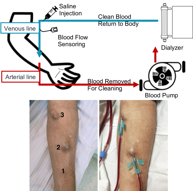
Figure 1: Hemodialysis process, blood flow detection, and positioning of auscultation sites.

1.2.4 Limited sample size

The evaluation of AVF was typically conducted by healthcare professionals, and often only the assessment results were recorded. The use of stethoscope recordings was not a regular practice. Furthermore, the collection of stethoscope recordings required a quiet room to minimize background noise. The quality of the stethoscope and the recording equipment could also impact data collection and study quality. As a result, the collection of stethoscope recordings during AVF auscultation was typically done in a trial-based scenario, which added to the practical burden and resulted in a limited number of sampled data. The recruited patient sizes in the studies ranged from 5 to 74 [5, 11, 12, 13, 14, 26, 27, 28, 29], which is considered small sample size for machine learning applications.

To address the aforementioned constraints in current research, this study employs deep neural networks to overcome the challenges with the following design:

1. Initially, a pretrain model is trained for dimensionality reduction and reconstruction. The latent representation learned from this model serves as efficient acoustic features, accommodating the non-stationary and patient-specific characteristics of auscultation recordings. The generalizability of this representation is also assessed.

2. Blood flow measurement, a widely recognized indicator for vascular access, exhibits strong predictive power in early detection of dysfunction and AVF complications [7]. Hence, it is adopted as the prediction label in this study.

3. Information from different puncture sites is analyzed, and the combination of latent information is explored.

4. To mitigate the limitation of a small dataset and enhance robust representation learning, a noise-mixing approach is employed to augment the dataset.

5. Considering the applicability of the proposed method to lightweight devices with limited computational capabilities, such as stethoscopes or wearable devices, a further dimensionality reduction technique is demonstrated while preserving approximate predictive ability.

2 Methods

In this study, we propose a representation learning approach based on the architecture of a deep denoising autoencoder (DAE), as depicted in Fig.2. The DAE is trained to perform dimensionality reduction and reconstruction tasks using the waveform of one-level coefficients obtained after applying discrete wavelet transform (DWT). The latent representation generated by the DAE is utilized for phono-angiography analysis in the downstream task.

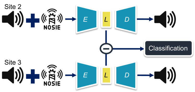
Figure 2: Model architecture DAE. $E$: encoder; $D$: decoder; $L$: latent representation; $\ominus$: subtraction of the two latent representation.

2.1 Deep autoencoder and deep denoising autoencoder

Deep autoencoder (AE) neural networks [30] are feed-forward multi-layer neural networks that aim to reconstruct the input data itself. The AE consists of an encoder and a decoder. The encoder, denoted as $f_{\theta}$, transforms the input $x$ into a hidden representation $y$ through a deterministic mapping:

$$f_{\theta}(x)=s(Wx+b),$$ (1)

where $s(\cdot)$ is a non-linear activation function, and $\theta=\{W,b\}$ represents the weights and biases of the encoder. The decoder, denoted as $g_{\theta^{\prime}}$, reconstructs the hidden representation $y$ into a latent space $z$:

$$z=g_{\theta^{\prime}}(y)=s(W^{\prime}y+b^{\prime}),$$ (2)

where $\theta^{\prime}=\{W^{\prime},b^{\prime}\}$ represents the weights and biases of the decoder. The goal of the autoencoder is to minimize the discrepancy between the original input $x$ and its reconstructed output $z$ [31].

The constraint of reducing dimensionality at the bottleneck layer separates useful information from noise and less informative details. This dimensionality reduction helps remove irrelevant variations and focuses on the essential aspects of the data, enhancing classification performance. By training an AE on a reconstruction task, the bottleneck layer becomes specialized in encoding discriminative features, which can be highly informative for other classification tasks.

DAE takes a further approach to reconstruction by considering noisy inputs [32, 33]. The DAE introduces a noise-adding step to the initial input $x$, denoted as noisy input $\widetilde{x}$. The encoder then maps $\widetilde{x}$ to a hidden representation:

$$y=f_{\theta}(\widetilde{x})=s(W\widetilde{x}+b).$$ (3)

The decoder reconstructs the clean input $x$ from the hidden representation $y$:

$$z=g_{\theta^{\prime}}(y).$$ (4)

The parameters $\theta$ and $\theta^{\prime}$ are trained to minimize the average reconstruction error over a training set, aiming to make the reconstructed output $z$ as close as possible to the clean input $x$.

The use of a denoising autoencoder allows the model to learn robust representations that are less sensitive to noise and variations in the input data. It can help to capture essential features while discarding irrelevant details and noise, leading to improved classification performance.

2.2 Experimental design

2.2.1 Patient recruitment

Patients were recruited from the HD unit of Chung-Hsin General Hospital. The inclusion criteria for the study were patients with functioning AVFs who were undergoing regular HD treatment. Exclusion criteria included age younger than 20 years, unwillingness or inability to undergo scheduled exams or follow-up regularly, and inability to provide written informed consent. After enrollment, electronic stethoscopes were used to collect auscultation signals at three sites of a mature AVF: arteriovenous anastomosis (site 1), arterial puncture site (site 2), and venous puncture site (site 3). The relative positions of these sites are shown in Fig. 1. AVF blood flows were measured using a Transonic® Flow-QC® Hemodialysis Monitor, which introduced saline into the venous line with the dialysis lines in a normal position. Recirculation was calculated based on the change in blood concentration between the venous sensor and arterial sensor [34]. The study was approved by the institutional review board of Chung-Hsin General Hospital (817) 109A-56, and all procedures were conducted in accordance with the principles outlined in the Declaration of Helsinki. Informed written consent was obtained from all participants prior to enrollment.

Since the measured blood flow indicates the vessel access between site 2 and 3, this research focused on the auscultation recordings from site 2 and 3. A total of 199 patients were initially recruited, but patients who lacked labels or had incomplete recordings (e.g., lack of recordings from site 2 or 3) were excluded from the analysis. Ultimately, 171 patients were included in the study. The blood flow detection task was designed as a three-class classification, categorizing blood flow into $<$750 ml/min, 750-1500 ml/min, and $>$1500 ml/min, representing different clinical requirements for HD patients.

2.2.2 Data preprocessing

The audio files were saved in the waveform audio file format (.wav) and digitized using a 16-bit analog-to-digital converter with a sample rate of 8 kHz. Preprocessing steps were applied to the audio recordings as follows: (1) Blank gaps before and after the auscultation sounds were removed. (2) The amplitude of the recordings was normalized. (3) The middle part of the recordings was segmented to avoid artifacts caused by placing and removing the stethoscope.

To extract pitch-specific acoustic features, the DWT was applied using a biorthogonal wavelet. Three levels of coefficients were obtained after the low-pass filter (LPF) and were denoted as $w_{L1}$, $w_{L2}$, and $w_{L3}$. The waveform, FFT, and STFT were computed for the original signal and the three level coefficients, as shown in Fig. 3. The FFT and STFT representations were then normalized using the absolute values and the natural logarithm of one plus the input ($log1p$) transformation. The $log1p$ transformation ensures that the values are above zero and normalizes potential errors that could be introduced by the distribution between positive and negative values [35, 36].

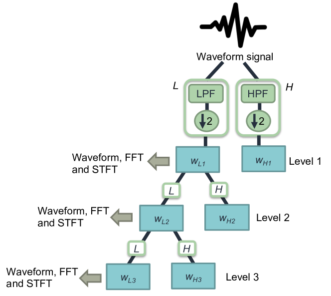
Figure 3: Wavelet transform process. L: low-pass filter (LPF) + downsampling; H: high-pass filter (HPF) + downsampling; $\downarrow$2: downsampling by the factor of 2; $w_{L1}$: one-level low-pass filtered coefficients; $w_{L2}$: two-level low-pass filtered coefficients; $w_{L3}$: three-level low-pass filtered coefficients; $w_{H1}$: one-level high-pass filtered coefficients; $w_{H2}$: two-level high-pass filtered coefficients; $w_{H3}$: three-level high-pass filtered coefficients; FFT: fast fourier transform; STFT: short-time fourier transform.

To overcome the limitation of a small number of samples, the auscultation audio recordings were mixed with seven different types of noise, including five colored noises (white, blue, violet, brown, and pink noises) and two types of background noise with people talking. The noise was added at two different volumes, resulting in a total of 2,394 mixed noisy auscultation recordings for site 2 and 3, respectively.

2.2.3 Model design

The architecture of the encoder and decoder for one-dimensional signals, which include waveform and FFT, consisted of three layers of fully-connected layers with Leaky Rectified Linear Unit (LeakyReLU) activation functions between each layer. The output sizes of the encoder layers were set to 5000, 1000, and 100, while the decoder layers had output sizes of 100, 1000, and 5000. For two-dimensional signals such as STFT, the architecture involved three layers of one-dimensional Convolutional (Conv1D) layers and max-pooling layers with Rectified Linear Unit (ReLU) activation functions between them. The encoder layers had filter sizes of 64, 32, and 16, and the decoder layers had filter sizes of 16, 32, and 64. The kernel sizes for the max-pooling layers were set to 2. The model was trained using the Adam optimizer and the mean squared error (MSE) loss function, aiming to minimize the discrepancy between the input and output. As the downstream task involved a small number of samples, the training was based on a Radial Basis Function (RBF)-kerneled Support Vector Machine (SVM) [37, 38]. The cost parameter ($C$) was set to 10 for the SVM.

2.2.4 Training strategies and classification metrics

The data were initially split into training and testing datasets for the pretraining of the encoder and decoder. The latent representation generated during the testing phase served as the dataset for training the downstream task. This dataset was then further divided into training and testing sets after balanced sampling. All downstream tasks were performed based on balanced sampling. The training process is illustrated in Fig. 4.

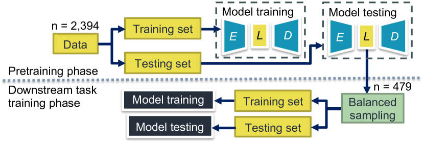
Figure 4: Model training process. $E$: encoder; $D$: decoder; $L$: latent representation; n: number of samples.

The quality of the learned latent representation was assessed using discrimination analysis. The autoencoder (AE) was set as the baseline and trained to reconstruct both the original clean signals (clean-to-clean) and the noise-mixed signals (noisy-to-noisy). The comparison between the two reconstructions indicated the effectiveness of enlarging the dataset. Additionally, the DAE was compared as it reconstructed clean audio from noisy audio, demonstrating the effectiveness of the asymmetric input and output approach.

To conduct a comprehensive analysis, various feature extraction methods proposed previously were tested for blood flow detection, including S-transform [13], IMF [14, 39], and Mel spectrogram [26]. The latent representation from different combinations of sites 2 and 3 were examined, as well as their individual representations. Furthermore, the generalization ability of the latent representation was assessed by predicting patient-specific information such as gender, hypertension (HTN) diagnosis, and diabetes mellitus (DM) diagnosis.

To achieve further dimensionality reduction on portable devices, the latent representation was condensed using principal component analysis (PCA) to lower dimensionalities. It was then concatenated with demographic information, including gender, age, HTN, and DM, as shown in Fig. 5. Categorical variables were encoded using one-hot encoding, and numeric variables were normalized using the $log1p$ function. Three algorithms based on different mechanisms were examined: SVM, k-nearest neighbors (KNN) [40], and Light Gradient Boosting Machine (LightGBM) [41]. The number of cluster in KNN were set to 3; The number of boosted trees in LightGBM was set to 100, and the learning rate was set to 0.05.

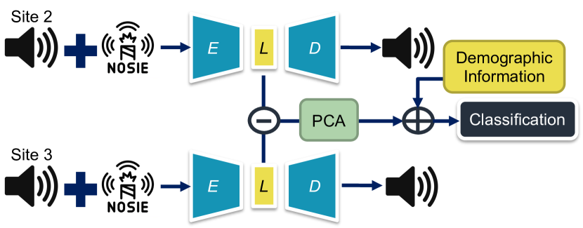
Figure 5: Model architecture DAE multi-modality combination. $E$: encoder; $D$: decoder; $L$: latent representation; $\ominus$: subtraction of the two latent representation; $\oplus$: concatenation of the two latent representation; PCA: principal component analysis.

The reported classification metrics included the area under the receiver operating characteristic (AUROC) curve, accuracy, sensitivity, specificity, precision, and F1 score [42]. These metrics were calculated by averaging the performance over ten runs of the training and testing process. Taking the mean performances of the testing samples over multiple runs was considered more representative than a single validation result. Since all the metrics are percentage indicators and higher scores represent better performance, a general average score (Avg.) was calculated to provide an overall measure of performance across all metrics. This helps assess the overall performance of the model.

3 Results

Table 1 showcases the demographic profile of the recruited patients. A majority of the recruited patients were of the male gender (59.65%), with diagnoses of HTN (72.52%) and DM (64.91%). The average age of the patients was 67 years, with the majority falling within the range of adequate blood flow (47.95%). Fig. 6 showcases the visualization of an audio sample in its original form, as well as $w_{L1}$, $w_{L2}$, and $w_{L3}$, respectively. Each level progressively filters out more information from the higher frequency band.

Table 1: Demographic information of recruit patients

Items		Values
Gender (n, %)	Male	102	(59.649)
	Female	69	(40.351)
Age (mean, SD)		67.596	13.279
HTN (n, %)	Yes	124	(72.515)
	No	47	(27.485)
DM (n, %)	Yes	111	(64.912)
	No	60	(35.088)
Blood Flow (ml/min) (n, %)	$<$ 750	45	(26.316)
	750-1500	82	(47.953)
	$>$ 1500	44	(25.731)
HTN: diagnosed with hypertension; DM: diagnosed with diabetes mellitus. n: number of recruit patients; SD: standard deviation.

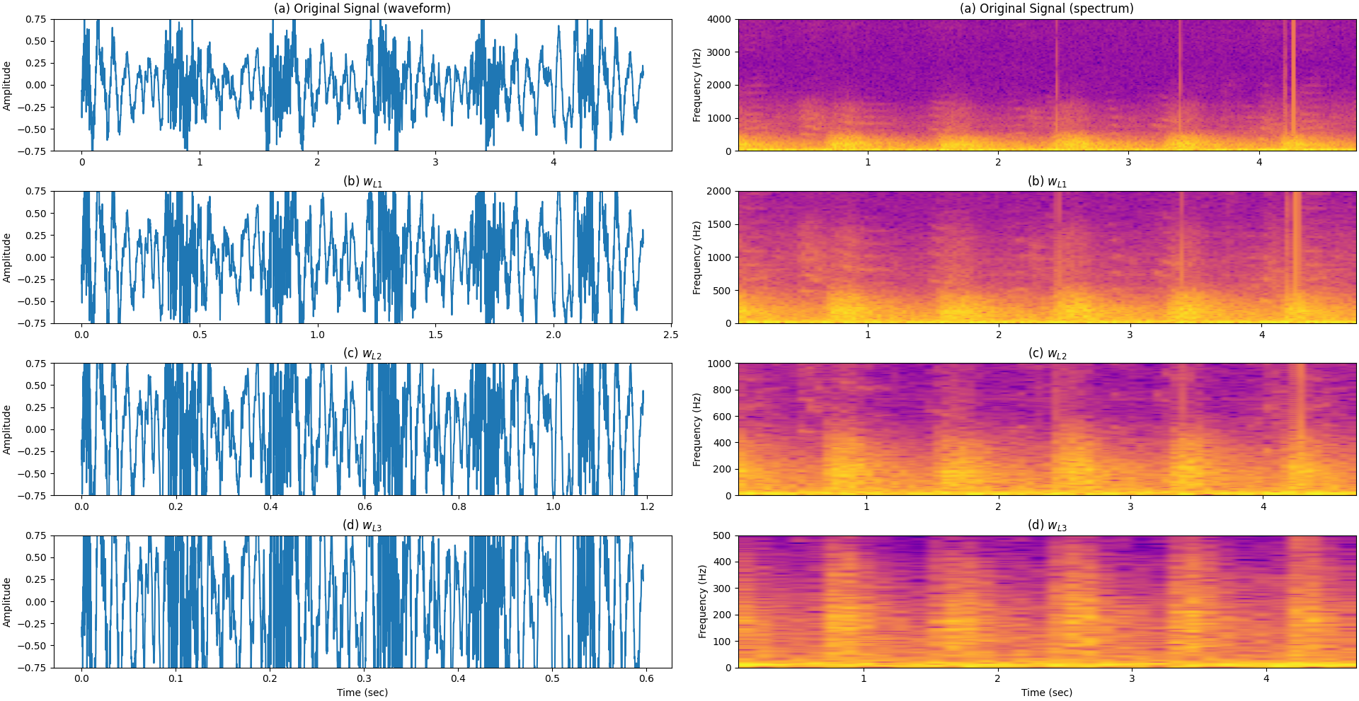
Figure 6: Wavelet transform from level 1 to 3. $w_{L1}$: one-level low-pass filtered coefficients; $w_{L2}$: two-level low-pass filtered coefficients; $w_{L3}$: three-level low-pass filtered coefficients.

By comparing Table 2(a) (n = 171) with (b) (n = 2,394), it becomes evident that augmenting the dataset through the noise-mixing approach proves to be efficient and significantly enhances the discrimination capabilities of the latent representation. Furthermore, a comparison between Table 2(b) and (c) highlights the impact of an asymmetric input and output. It is noteworthy that the noise-to-clean scheme exhibits the ability to improve performance. Employing a lower level of DWT does not necessarily lead to performance improvement.

The most exceptional latent representation, which serves as the baseline for subsequent comparisons, is generated by the DAE using $w_{L1}$, achieving an average score of 0.95. The representations learned from the waveform, FFT, and STFT of $w_{L1}$ were compared (presented in Table 3). The results indicate that the waveform is the most viable feature for generating a discriminative latent representation for downstream task classification.

Table 2: The effect of adding noise and different AE structure

	Original	$w_{L1}$	$w_{L2}$	$w_{L3}$
	(a) AE waveform (clean to clean)
AUROC	0.508	0.498	0.601	0.655
Accuracy	0.311	0.278	0.189	0.278
Sensitivity	0.313	0.343	0.239	0.393
Specificity	0.668	0.668	0.640	0.669
Precision	0.304	0.277	0.233	0.287
F1	0.276	0.246	0.176	0.269
Avg.	0.397	0.385	0.346	0.425
	(b) AE waveform noise-mixing version (noisy to noisy)
AUROC	0.990	0.977	0.989	0.976
Accuracy	0.908	0.886	0.894	0.875
Sensitivity	0.906	0.886	0.901	0.872
Specificity	0.953	0.944	0.948	0.936
Precision	0.910	0.893	0.905	0.872
F1	0.904	0.883	0.893	0.867
Avg.	0.929	0.912	0.922	0.900
	(c) DAE waveform noise-mixing version (noisy to clean)
AUROC	0.993	0.987	0.989	0.990
Accuracy	0.922	0.933	0.878	0.911
Sensitivity	0.923	0.935	0.891	0.915
Specificity	0.964	0.967	0.941	0.956
Precision	0.915	0.932	0.884	0.909
F1	0.913	0.932	0.876	0.908
Avg.	0.938	0.948	0.910	0.931
$w_{L1}$: one-level low-pass filtered coefficients; $w_{L2}$: two-level low-pass filtered coefficients; $w_{L3}$: three-level low-pass filtered coefficients. AE: autoencoder; DAE: denoising autoencoder; AUROC: area under the receiver operating characteristic curve.

Table 3: Classification results between different features

	Original	$w_{L1}$	$w_{L2}$	$w_{L3}$
	DAE + waveform
AUROC	0.993	0.987	0.989	0.990
Accuracy	0.922	0.933	0.878	0.911
Sensitivity	0.923	0.935	0.891	0.915
Specificity	0.964	0.967	0.941	0.956
Precision	0.915	0.932	0.884	0.909
F1	0.913	0.932	0.876	0.908
Avg.	0.938	0.948	0.910	0.931
	DAE + FFT
AUROC	0.909	0.964	0.943	0.934
Accuracy	0.772	0.864	0.869	0.839
Sensitivity	0.772	0.863	0.869	0.834
Specificity	0.888	0.932	0.935	0.919
Precision	0.770	0.866	0.872	0.840
F1	0.762	0.860	0.863	0.832
Avg.	0.812	0.892	0.892	0.866
	DAE + STFT
AUROC	0.923	0.926	0.904	0.832
Accuracy	0.786	0.794	0.775	0.622
Sensitivity	0.794	0.795	0.780	0.622
Specificity	0.893	0.897	0.890	0.812
Precision	0.783	0.791	0.787	0.618
F1	0.781	0.789	0.770	0.607
Avg.	0.827	0.832	0.818	0.685
FFT: fast fourier transform; STFT: short time fourier transform; DAE: denoising autoencoder; $w_{L1}$: one-level low-pass filtered coefficients; $w_{L2}$: two-level low-pass filtered coefficients; $w_{L3}$: three-level low-pass filtered coefficients. DAE: denoising autoencoder; AUROC: area under the receiver operating characteristic curve.

Table 4(a) presents the outcomes obtained by applying previously proposed methods in our scenario. However, none of these methods exhibited sufficient distinctiveness for AVF blood flow detection. In Table 4(b), we showcase the downstream task performance based on the representation of individual sites as well as the subtraction of site 2-3. While each individual site achieved a satisfactory accuracy of 0.90, the subtraction of site 2-3 surpassed other combinations, such as concatenation and addition. Table 4(c) provides an overview of the performance when patient-specific information was set as the classification target. All approaches yielded commendable performance, surpassing an average score of 0.93.

Utilizing the original latent representation (dim = 100) as a reference, Table 4(d) exhibits the outcomes obtained by reducing the dimensionality to 5, 4, and 2. As the dimensionality decreased, the performance also declined. However, when the condensed representation (dim = 2) is concatenated with the demographic information, the performance can be restored to a level approximating the best-performing version using LightGBM, as illustrated in Table 4(e). Fig. 7 provides a visualization of the feature importance as determined by the tree-based algorithm employed for branching. The results indicate that the model places the highest value on the condensed representation, followed by age, the presence of DM, gender, and HTN diagnosis.

Table 4: Additional examinations

(a) Feature extraction from previous research (based on $w_{L1}$ of site 2).
	S-transform [13]	IMF [14]	Mel spectrogram [26]
AUROC	0.639	0.623	0.656
Accuracy	0.443	0.365	0.513
Sensitivity	0.451	0.385	0.517
Specificity	0.725	0.689	0.761
Precision	0.463	0.472	0.528
F1	0.440	0.360	0.509
Avg.	0.527	0.482	0.581
(b) Validation results based on single and multiple sites (based on $w_{L1}$).
	Site 2	Site 3	Site 2-3
AUROC	0.990	0.981	0.987
Accuracy	0.906	0.903	0.933
Sensitivity	0.906	0.906	0.935
Specificity	0.953	0.952	0.967
Precision	0.910	0.904	0.932
F1	0.903	0.901	0.932
Avg.	0.928	0.925	0.948
(c) Classification on patient information.
	Gender	HTN	DM
AUROC	0.990	0.996	0.993
Accuracy	0.920	0.950	0.923
Sensitivity	0.887	0.933	0.923
Specificity	0.951	0.968	0.927
Precision	0.947	0.966	0.934
F1	0.914	0.947	0.925
Avg.	0.935	0.960	0.937
(d) PCA results (based on $w_{L1}$ of site 2-3)
	dim = 5	dim = 4	dim = 2
AUROC	0.887	0.879	0.770
Accuracy	0.756	0.747	0.614
Sensitivity	0.765	0.747	0.605
Specificity	0.880	0.874	0.805
Precision	0.761	0.751	0.624
F1	0.750	0.740	0.586
Avg.	0.800	0.790	0.667
(e) Concatenated with demographic information
	SVM	KNN	LightGBM
AUROC	0.768	0.928	0.957
Accuracy	0.569	0.842	0.906
Sensitivity	0.580	0.838	0.904
Specificity	0.787	0.918	0.952
Precision	0.592	0.850	0.915
F1	0.556	0.836	0.900
Avg.	0.642	0.869	0.922
Site 1: site of arteriovenous anastamosis; Site 2: arterial puncture site; Site 3: venous puncture site; Site 2-3: subtracting the latent representation of site 3 from site 2. IMF: intrinsic mode function; HTN: diagnosed with hypertension; DM: diagnosed with diabetes mellitus; dim: condensed dimensionality; SVM: support vector machine, KNN: k-nearest neighbors; LightGBM: light gradient-boosting machine; $w_{L1}$: one-level low-pass filtered coefficients; AUROC: area under the receiver operating characteristic curve. Note that in (e) the concatenation was based on the latent features of $w_{L1}$ of site 2-3 condensing to dim = 2.

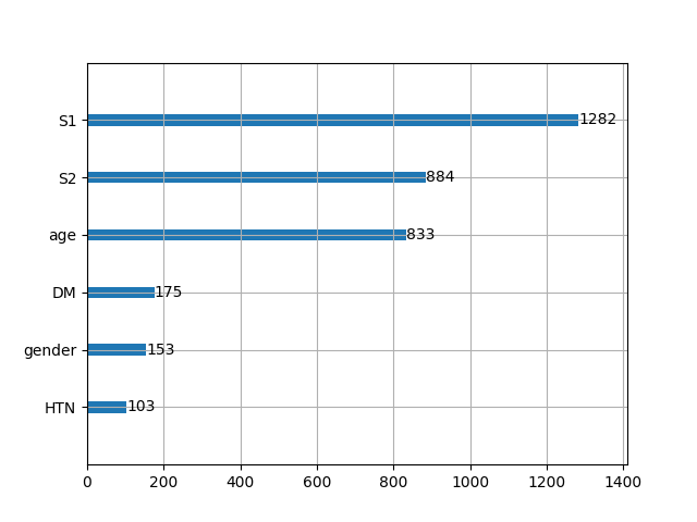
Figure 7: Feature importance of LightGBM. LightGBM: light gradient-boosting machine; S1: dimensional 1 of the condensed signal; S2: dimensional 2 of the condensed signal; HTN: diagnosed with hypertension; DM: diagnosed with diabetes mellitus.

4 Discussion

Prior investigations [32] have underscored the perils of training deep neural network models directly on the supervised target through gradient descent, as random initialization may not yield optimal performance. Conversely, commencing the training process with a pre-trained model has demonstrated its efficacy in enhancing generalization. In our study, we employed DAEs to generate a distinctive representation well-suited for detecting blood flow. Our findings indicate that representation learning presents a more viable approach for extracting auscultation features in AVF. Feature extraction methods based on signal characteristics may exhibit high specificity to particular prediction scenarios and lack ease of transferability to other contexts. In contrast, the acquired latent representation showcases improved generalization and applicability in non-extreme contrast scenarios (e.g., stenosis and non-stenosis) as well as other patient-specific characteristics. While our study did not simultaneously collect different access indicators, such as RI or luminal diameter, to validate transferability, our findings suggest that a well-learned representation captures additional patient-specific information that can be transferred to multiple tasks. Furthermore, AVF blood flow serves as a more comprehensive measurement aligning with the need for early surveillance and supporting the detection of stenosis and other dysfunctions [22, 17]. Additionally, we have successfully applied the proposed architecture to pathological voice quality detection, yielding satisfactory outcomes [43].

Effective representation learning necessitates a sufficient amount of data. Despite our relatively large sample size of recruited patients, the original clean signal alone was insufficient to generate a well-learned representation. However, augmentation methods, such as the noise-mixing approach, offer a simple and feasible solution to overcome limitations in data size. Forcing the model to reconstruct the clean signal from the noisy signal proves to be an effective approach for generating a more representative representation. Our results demonstrate that the time domain information captured in the waveform is adequate for generating a well-learned representation, whereas the frequency domain information and time-dependent windows converted using FFT and STFT do not appear to be essential. Previous studies have also highlighted the sufficiency of time domain information for turbulent sound analysis [44], while additional information in the FFT window may introduce noise and lead to averaging within [28]. The fixed window width of STFT may not be ideal for accurately tracking dynamic signals [13]. Moreover, the inclusion of additional, less informative details can impede precise reconstruction, thereby generating a less representative representation. While a one-level DWT discards less informative details, excessive information loss (e.g., $w_{L3}$) hampers prediction performance.

The intensity of the bruit is most pronounced near the arterial anastomosis (site 1), followed by the arterial and venous puncture sites (site 2 and 3). Subtracting the latent representation of site 3 from site 2 effectively indicates the blood flow loss in between, thus demonstrating distinguishable results. Previous works [45, 46] have demonstrated the possibility of reconstructing diverse images of real subjects through interpolations in latent space, highlighting the feasibility of manipulating latent representations to generate targeted outcomes.

Excessive dimensionality reduction at the bottleneck of AEs may hinder reconstruction performance. Consequently, we opted to condense the dimensionality after generating adequate representations. Our results illustrate that prediction performance can be restored by concatenating a vector of six elements using an appropriate machine learning method. The concatenated vector comprises heterogeneous information, necessitating the identification of a threshold to discriminate between different categories. This task can be effectively handled by tree-based algorithms [47]. The condensed representation continues to exhibit greater discriminative power compared to other variables, as indicated by its high value in tree-based algorithms. Furthermore, numeric variables tend to demonstrate higher discriminative capability than categorical variables.

5 Conclusion

Our study showcased the effectiveness of representation learning using DAEs for non-invasive AVF blood flow detection. This approach proved to be highly accurate and capable of capturing patient-specific information, enabling its application in various contexts. Furthermore, the learned representations maintained high performance even under highly condensed conditions. The manipulation of latent representations holds great promise for future advancements. Further exploration of the generated latent representation can enhance the development of smart stethoscopes and pave the way for future applications.

References

- [1] R. Navuluri and S. Regalado, “The KDOQI 2006 vascular access update and fistula first program synopsis,” in Seminars in interventional radiology, vol. 26, no. 02, 2009, pp. 122–124.
- [2] M. C. Riella and P. Roy-Chaudhury, “Vascular access in haemodialysis: strengthening the achilles’ heel,” Nature Reviews Nephrology, vol. 9, no. 6, pp. 348–357, 2013.
- [3] A. A. Al-Jaishi, M. J. Oliver, S. M. Thomas, C. E. Lok, J. C. Zhang, A. X. Garg, S. D. Kosa, R. R. Quinn, and L. M. Moist, “Patency rates of the arteriovenous fistula for hemodialysis: A systematic review and meta-analysis,” American Journal of Kidney Diseases, vol. 63, no. 3, pp. 464–478, 2014.
- [4] N. Koirala, E. Anvari, and G. McLennan, “Monitoring and surveillance of hemodialysis access,” in Seminars in interventional radiology, vol. 33, no. 01. Thieme Medical Publishers, 2016, pp. 025–030.
- [5] D.-F. Yeih, Y.-S. Wang, Y.-C. Huang, M.-F. Chen, and S.-S. Lu, “Physiology-based diagnosis algorithm for arteriovenous fistula stenosis detection,” in 2014 36th Annual International Conference of the IEEE Engineering in Medicine and Biology Society, 2014, pp. 4619–4622.
- [6] K. Abreo, B. M. Amin, and A. P. Abreo, “Physical examination of the hemodialysis arteriovenous fistula to detect early dysfunction,” The Journal of Vascular Access, vol. 20, no. 1, pp. 7–11, 2019.
- [7] R. Peralta, M. Garbelli, F. Bellocchio, P. Ponce, S. Stuard, M. Lodigiani, J. Fazendeiro Matos, R. Ribeiro, M. Nikam, M. Botler et al., “Development and validation of a machine learning model predicting arteriovenous fistula failure in a large network of dialysis clinics,” International Journal of Environmental Research and Public Health, vol. 18, no. 23, p. 12355, 2021.
- [8] C. E. Lok, T. S. Huber, T. Lee, S. Shenoy, A. S. Yevzlin, K. Abreo, M. Allon, A. Asif, B. C. Astor, M. H. Glickman et al., “KDOQI clinical practice guideline for vascular access: 2019 update,” American Journal of Kidney Diseases, vol. 75, no. 4, pp. S1–S164, 2020.
- [9] ——, “KDOQI clinical practice guideline for vascular access: 2019 update,” American Journal of Kidney Diseases, vol. 75, no. 4, pp. S1–S164, 2020.
- [10] A. M. Noor, “Non-imaging acoustical properties in monitoring arteriovenous hemodialysis access. a review.” Journal of Engineering & Technological Sciences, vol. 47, no. 6, 2015.
- [11] P. O. Vesquez, M. M. Marco, and B. Mandersson, “Arteriovenous fistula stenosis detection using wavelets and support vector machines,” in 2009 Annual International Conference of the IEEE Engineering in Medicine and Biology Society, 2009, pp. 1298–1301.
- [12] D. Higashi, K. Nishijima, K. Furuya, K. Tanaka, and S. Shin, “Classification of shunt murmurs for diagnosis of arteriovenous fistula stenosis,” in 2018 Asia-Pacific Signal and Information Processing Association Annual Summit and Conference (APSIPA ASC), 2018, pp. 665–669.
- [13] H.-Y. Wang, C.-H. Wu, C.-Y. Chen, and B.-S. Lin, “Novel noninvasive approach for detecting arteriovenous fistula stenosis,” IEEE Transactions on Biomedical Engineering, vol. 61, no. 6, pp. 1851–1857, 2014.
- [14] P. Vásquez, M. M. Marco, E. Mattsson, and B. Mandersson, “Application of the empirical mode decomposition in the study of murmurs from arteriovenous fistula stenosis,” in 2010 Annual International Conference of the IEEE Engineering in Medicine and Biology, 2010, pp. 947–950.
- [15] Y. Bengio, A. Courville, and P. Vincent, “Representation learning: A review and new perspectives,” IEEE transactions on pattern analysis and machine intelligence, vol. 35, no. 8, pp. 1798–1828, 2013.
- [16] D. Zhang, J. Yin, X. Zhu, and C. Zhang, “Network representation learning: A survey,” IEEE transactions on Big Data, vol. 6, no. 1, pp. 3–28, 2018.
- [17] K. Konner, B. Nonnast-Daniel, and E. Ritz, “The arteriovenous fistula,” Journal of the American Society of Nephrology, vol. 14, no. 6, pp. 1669–1680, 2003.
- [18] N. Tessitore, G. Lipari, A. Poli, V. Bedogna, E. Baggio, C. Loschiavo, G. Mansueto, and A. Lupo, “Can blood flow surveillance and pre-emptive repair of subclinical stenosis prolong the useful life of arteriovenous fistulae? a randomized controlled study,” Nephrology Dialysis Transplantation, vol. 19, no. 9, pp. 2325–2333, 2004.
- [19] N. Tessitore, V. Bedogna, A. Poli, W. Mantovani, G. Lipari, E. Baggio, G. Mansueto, and A. Lupo, “Adding access blood flow surveillance to clinical monitoring reduces thrombosis rates and costs, and improves fistula patency in the short term: a controlled cohort study,” Nephrology Dialysis Transplantation, vol. 23, no. 11, pp. 3578–3584, 2008.
- [20] G. A. Miller and W. W. Hwang, “Challenges and management of high-flow arteriovenous fistulae,” in Seminars in nephrology, vol. 32, no. 6. Elsevier, 2012, pp. 545–550.
- [21] P. N. Suding and S. E. Wilson, “Strategies for management of ischemic steal syndrome,” in Seminars in vascular surgery, vol. 20, no. 3. Elsevier, 2007, pp. 184–188.
- [22] P. Mccarley, R. L. Wingard, Y. Shyr, W. Pettus, R. M. Hakim, and T. A. Ikizler, “Vascular access blood flow monitoring reduces access morbidity and costs,” Kidney international, vol. 60, no. 3, pp. 1164–1172, 2001.
- [23] W.-L. Chen, C.-D. Kan, and C.-H. Lin, “Arteriovenous shunt stenosis evaluation using a fractional-order fuzzy petri net based screening system for long-term hemodialysis patients,” Journal of Biomedical Science and Engineering, vol. 2014, 2014.
- [24] M. Grochowina and L. Leniowska, “Design and implementation of a device supporting automatic diagnosis of arteriovenous fistula,” in 2018 Signal Processing: Algorithms, Architectures, Arrangements, and Applications (SPA), 2018, pp. 186–190.
- [25] Y.-N. Wang, C.-Y. Chan, and S.-J. Chou, “The detection of arteriovenous fistula stenosis for hemodialysis based on wavelet transform,” International Journal of Advanced Computer Science, vol. 1, no. 1, pp. 16–22, 2011.
- [26] J. H. Park, I. Park, K. Han, J. Yoon, Y. Sim, S. J. Kim, J. Y. Won, S. Lee, J. H. Kwon, S. Moon, G. M. Kim, and M.-D. Kim, “Feasibility of deep learning-based analysis of auscultation for screening significant stenosis of native arteriovenous fistula for hemodialysis requiring angioplasty,” Korean J Radiol. 2022 Oct;23(10):949-958., vol. 10, 2022.
- [27] M. M. Munguía and B. Mandersson, “Analysis of the vascular sounds of the arteriovenous fistula’s anastomosis,” in 2011 Annual International Conference of the IEEE Engineering in Medicine and Biology Society, 2011, pp. 3784–3787.
- [28] M. Grochowina, K. Wojnar, and L. Leniowska, “An application of wavelet transform for non-invasive evaluation of arteriovenous fistula state,” in 2019 Signal Processing: Algorithms, Architectures, Arrangements, and Applications (SPA), 2019, pp. 214–217.
- [29] K. Ota, Y. Nishiura, S. Ishihara, H. Adachi, T. Yamamoto, and T. Hamano, “Evaluation of hemodialysis arteriovenous bruit by deep learning,” Sensors, vol. 20, no. 17, 2020.
- [30] K.-H. Tsai, W.-C. Wang, C.-H. Cheng, C.-Y. Tsai, J.-K. Wang, T.-H. Lin, S.-H. Fang, L.-C. Chen, and Y. Tsao, “Blind monaural source separation on heart and lung sounds based on periodic-coded deep autoencoder,” IEEE Journal of Biomedical and Health Informatics, vol. 24, no. 11, pp. 3203–3214, 2020.
- [31] G. E. Hinton and R. R. Salakhutdinov, “Reducing the dimensionality of data with neural networks,” Science, vol. 313, no. 5786, pp. 504–507, 2006.
- [32] P. Vincent, H. Larochelle, I. Lajoie, Y. Bengio, P.-A. Manzagol, and L. Bottou, “Stacked denoising autoencoders: Learning useful representations in a deep network with a local denoising criterion.” Journal of machine learning research, vol. 11, no. 12, 2010.
- [33] X. Lu, Y. Tsao, S. Matsuda, and C. Hori, “Speech enhancement based on deep denoising autoencoder.” in Interspeech, vol. 2013, 2013, pp. 436–440.
- [34] Transonic, “HD03 hemodialysis monitor.” [Online]. Available: https://www.transonic.com/hd03-monitor
- [35] Y.-J. Lu, C.-F. Liao, X. Lu, J.-w. Hung, and Y. Tsao, “Incorporating broad phonetic information for speech enhancement,” arXiv preprint arXiv:2008.07618, 2020.
- [36] S.-Y. Chuang, H.-M. Wang, and Y. Tsao, “Improved lite audio-visual speech enhancement,” IEEE/ACM Transactions on Audio, Speech, and Language Processing, vol. 30, pp. 1345–1359, 2022.
- [37] B. Scholkopf, K.-K. Sung, C. Burges, F. Girosi, P. Niyogi, T. Poggio, and V. Vapnik, “Comparing support vector machines with gaussian kernels to radial basis function classifiers,” IEEE Transactions on Signal Processing, vol. 45, no. 11, pp. 2758–2765, 1997.
- [38] W. S. Noble, “What is a support vector machine?” Nature biotechnology, vol. 24, no. 12, pp. 1565–1567, 2006.
- [39] D. Laszuk, “Python implementation of empirical mode decomposition algorithm,” https://github.com/laszukdawid/PyEMD, 2017.
- [40] M.-L. Zhang and Z.-H. Zhou, “ML-KNN: A lazy learning approach to multi-label learning,” Pattern Recognition, vol. 40, no. 7, pp. 2038–2048, 2007.
- [41] G. Ke, Q. Meng, T. Finley, T. Wang, W. Chen, W. Ma, Q. Ye, and T.-Y. Liu, “LightGBM: A highly efficient gradient boosting decision tree,” Advances in neural information processing systems, vol. 30, 2017.
- [42] R. Parikh, A. Mathai, S. Parikh, G. C. Sekhar, and R. Thomas, “Understanding and using sensitivity, specificity and predictive values,” Indian journal of ophthalmology, vol. 56, no. 1, p. 45, 2008.
- [43] L.-C. Chen, Y.-H. Lin, W.-H. Tseng, C.-T. Tan, and Y. Tsao, “Autoencoder-based pathological voice classification,” 2023. [Online]. Available: https://ishiou.github.io/PathologyVoice/initialresults.html
- [44] Y. Akay, M. Akay, W. Welkowitz, J. Semmlow, and J. Kostis, “Noninvasive acoustical detection of coronary artery disease: a comparative study of signal processing methods,” IEEE Transactions on Biomedical Engineering, vol. 40, no. 6, pp. 571–578, 1993.
- [45] C. Donahue, Z. C. Lipton, A. Balsubramani, and J. McAuley, “Semantically decomposing the latent spaces of generative adversarial networks,” 2018.
- [46] T. Sainburg, M. Thielk, B. Theilman, B. Migliori, and T. Gentner, “Generative adversarial interpolative autoencoding: adversarial training on latent space interpolations encourage convex latent distributions,” 2019.
- [47] C. Kern, T. Klausch, and F. Kreuter, “Tree-based machine learning methods for survey research,” in Survey research methods, vol. 13, no. 1. NIH Public Access, 2019, p. 73.