Robust Topological Anderson Insulator Induced Reentrant Localization Transition

Abstract

We study the topology and localization properties of a generalized Su-Schrieffer-Heeger (SSH) model with a quasi-periodic modulated hopping. It is found that the interplay of off-diagonal quasi-periodic modulations can induce topological Anderson insulator (TAI) phases and reentrant topological Anderson insulator (RTAI), and the topological phase boundaries can be uncovered by the divergence of the localization length of the zero-energy mode. In contrast to the conventional case that the TAI regime emerges in a finite range with the increase of disorder, the TAI and RTAI are robust against arbitrary modulation amplitude for our system. Furthermore, we find that the TAI and RTAI can induce the emergence of reentrant localization transitions. Such an interesting connection between the reentrant localization transition and the TAI/RTAI can be detected from the wave-packet dynamics in cold atom systems by adopting the technique of momentum-lattice engineering.

I Introduction

Anderson localization is a ubiquitous phenomenon in the condensed matter where the wave-like behavior of particles becomes localized in a disordered medium, preventing their propagation. This phenomenon was first introduced by P. W. Anderson in 1958 and has since been observed in a wide range of physical platforms  Anderson1958 ; Ramakrishnan1985RMP , including electrons in solids, cold atoms Billy2008Nat ; Roati2008Nat , microwave cavities Chabanov2000Nat ; Pradhan2000PRL , and photonic lattices Lahini2009PRL . Anderson localization has significant implications for understanding transport features in disordered systems. For system dimensions $D\leq 2$, the single-parameter scaling theory predicts that an arbitrarily small on-site random disorder induces all states to be localized for non-interacting fermions Mott1987JPC . However, such a scaling theory is invalid in a quasi-periodic system, for which low-dimensional quasicrystals may exhibit a metal-to-insulator transition. The paradigmatic example is the Aubry-André (AA) model Aubry1980 ; Harper1955 ; Longhi2019PRL ; Longhi2019PRB , which has been experimentally realized in cold atoms Roati2008Nat and photonic crystals Kraus2012PRL ; Segev2013NP , which exhibits an extended-to-localized transition for all the eigenstates at a finite critical modulation amplitude determined by its self-dual characteristic. By breaking the self-duality of the AA model, one can obtain a localization transition through an intermediate phase with coexisting extended and localized states separated by a critical energy called the mobility edge (ME) Biddle2010PRL ; Ganeshan2015PRL , similar to the random disordered cases in three-dimensions. Moreover, quasi-periodic systems exhibit many unique properties, including their nontrivial connection to topological phases Kraus2012PRL and a variety of localization transitions between extended, localized, and critical phases XJL2022 ; XJL2023 ; TL2023 ; Sharma2021PRB1 ; Sharma2021PRB2 ; Sharma2022PRB1 ; TL2021PRB ; Wang2016PRB , as well as the emergence of the cascade-like delocalization transitions in the interpolating Aubry-André-Fibonacci model Goblot2020 ; ZZhai2021 .

It is generally understood that after the localization transition in a disordered system, the localized states remain localized as a function of the disorder amplitude. However, a recent study predicts a reentrant localization transition in a one-dimensional (1D) dimerized hopping model with a staggered quasi-periodic modulation SRoy2021PRL . Such a model can undergo two localization transitions,
which means the system first becomes localized as the disorder increases, at some critical point, some of the localized states go back to delocalized ones, and as the disorder further increases, the system again becomes localized. Both localization transitions are found to pass through two intermediate regimes with ME, four transition points emerging with the modulation amplitude increasing Padhan2022PRB ; SRoy2022PRB ; ZWZPRA2022 ; SA2023PRB . Such reentrant localization phenomena are also predicted in non-Hermitian systems and can be detected by wave-packet dynamics CWNJP2021 ; XPJ2021CPB ; LZhou2022PRB ; WH2022PRB ; HW2023PRB .

On the other hand, topological insulators, characterized by quantized electronic transport of charge for bulk states with nontrivial in-gap modes, have attracted broad interest in the last decades. Topology and disorder exhibit many fantastic connections, from the similarity of 1D quasi-periodic and two-dimensional Hofstadter lattices to the connection between the random matrix and the classification of topological phases Nakajima2021NP . One hallmark property of the topological insulators is the robustness of nontrivial edge states against weak disorder in the underlying lattice. This robustness is due to the fact that the quantized transport occurs along the edge states, which are immune to topologically protected backscattering. However, when the disorder amplitude is large enough, the band gap closes, and the system usually becomes trivial Su1979 ; Thouless1982 ; Hasan2010 ; QXliangRMP2011 ; BansilRMP2016 ; Chiu2016 ; ArmitageRMP2018 ; Prodan2010 ; Cai2013 ; Song2019PRL ; XZhao2020PRA1 ; Bo2021 . Conversely, the disorder can induce nontrivial topology when added into a trivial band system, known as the topological Anderson insulator (TAI), which is accompanied by the emergence of topologically protected edge modes and quantized topological charges Shen2009 ; Groth2009 . The TAI has been studied in various theoretical models Guo2010 ; Zhang2012 ; Song2012 ; Girschik2013 ; Hughes2014 ; Zhang2019 ; DZhang2020 ; Tangg2020 ; Borchmann2016 ; Hua2019 ; GQZ2021 ; Velury2021 ; SNL2022 ; YPW2022 ; WJZ2022 , and has been observed experimentally in various artificial systems such as two-dimensional photonics system Sttzer2018 ; Liu2020 and one-dimensional engineering synthetic 1D chiral symmetric wires Meier2018 . For a random disorder-induced TAI, one finds that the bulk states of the TAI are always localized. However, recent studies show that for a quasi-periodic modulation-induced TAI phase, the bulk states show unique localization behaviors Longhi2020 ; DZhang2022 .

This paper investigates a generalized SSH model with off-diagonal quasi-periodic modulations exhibiting exotic topological and localization phenomena. First, we numerically calculate the topological phase diagram by the real-space winding number to characterize the effects    of off-diagonal quasi-periodic modulations on topology. When the ratio of the site-independent intracell tunneling energy and the intercell one $v/w<0.6$, the nontrivially topological feature is robust against the modulation. For $0.6<v/w<1$, as the modulation increases, the system undergoes the topological phase transitions among nontrivial-trivial-nontrivial regions, which displays the emergence of the ”reentrant topological Anderson insulator” (RTAI). For $v/w>1$, a TAI can be induced by the quasi-periodic disorder. The RTAI and TAI phases in our system exhibit the robustness of the nontrivial topology against arbitrary large modulations. Such topological features are also characterized by the divergence of the zero mode’s localization length. Furthermore, we study the localization properties of our system and verify the existence of the reentrant localization transition. By comparing the localization and topological phase diagrams, we find that the reentrant localization transition coincides with the RTAI and TAI phase transitions, and a physical explanation is given. Finally, we illustrate that the relationship between the TAI and the reentrant localization transition can be detected by the wave-packet dynamics in the momentum-lattice system.

The structure of this paper is as follows: In Sec.ii@, we briefly introduce the Hamiltonian of the SSH model with off-diagonal quasi-periodic modulation. In Sec.iii@, we obtain the topological phase diagram and discuss the fate of topological zero-energy modes. We find the robustness of the topological properties against strong disorder in our model and the emergence of the TAI and RTAI phases. In Sec.iv@, we investigate the localization transition and present the localization phase diagram. Moreover, we discuss the connections between the TAI/RTAI and the reentrant localization transition. Furthermore, in Sec.v@, we apply wave-packet dynamics to detect the topology and localization transition in our model. Finally, we summarize our findings in Sec.vi@.

II Model and Hamiltonian

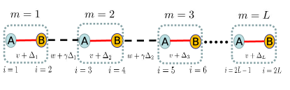
Figure 1: (Color online) Schematic illustration of the generalized quasi-periodic SSH model with two sublattices ($A$ and $B$) in each unit cell shown in the dotted box. This is a chain with $L$ unit cells, and the length of the chain is $2L$. Here, $m$ is the index of the unit cell, and $i$ represents the lattice site. $w+\gamma\Delta_{m}$ and $v+\Delta_{m}$ are the $m$-dependent intercell and intracell hopping amplitudes, respectively.

The reentrant localization transition is first observed in a SSH model with the staggered quasi-periodic on-site potential, which breaks the chiral symmetry of the SSH chain and is topologically trivial. To detect the relationship between the reentrant localization and the topological transition, we consider a generalized SSH model with quasi-periodic modulated hopping, which preserves the chiral symmetry and is depicted in Fig. 1. The dimerized tight-binding model can be described by

$$\small H=\sum_{m=1}^{L}v_{m}(c^{{\dagger}}_{m,B}c_{m,A}+H.c.)+\sum_{m=1}^{L-1}w_{m}(c^{{\dagger}}_{m+1,A}c_{m,B}+H.c.).$$ (1)

This is a chain of $L$ unit cells consisting of two sublattices labeled by $A$ and $B$, and the length of the lattice is $2L$. As shown in Fig. 1, $m$ is the index of the unit cell, and $i$ represents the lattice site. $c^{{\dagger}}_{m,A}$ ($c^{\dagger}_{m,B}$) is the creation operator for a particle on the $A$ ($B$) sublattice of the $m$th cell, and $c_{m,A}$ ($c_{m,B}$) is the corresponding annihilation operator. $v_{m}$ and $w_{m}$ characterize the intra- and inter-cell hopping amplitudes, respectively. This model describes a chiral chain with the Hamiltonian $H$ obeying $SH=-HS$. Here, the chiral operator $S=I_{L}\otimes\sigma_{z}$, where $\sigma_{z}$ is the Pauli matrix (sublattice space), and $I_{L}$ is a $L\times L$ identity matrix (unit-cell coordinate space). To preserve the chiral symmetry, we consider the quasi-periodic modulated intracell and intercell hoppings respectively with the amplitudes,

$$v_{m}=v+{\Delta_{m}},\quad w_{m}=w+\gamma{\Delta_{m}},$$ (2)

with

$${\Delta_{m}}={\Delta}\cos(2\pi\beta m+\phi).$$ (3)

Here, $v$ and $w$ are the site-independent intracell and intercell tunneling energies, $\Delta$ is the strength of the incommensurate modulation, $\gamma$ is the ratio of quasi-periodic modulations of intra- to intercell tunneling (here we consider $\gamma>1$), $\beta$ is an irrational number to ensure the incommensurate modulation, and $\phi\in[0,2\pi)$ is an arbitrary phase. In the clean case ($\Delta=0$), the Hamiltonian Eq. (1) reduces to a standard SSH model Su1979 . When the intracell hopping amplitude $v$ exceeds the intracell hopping amplitude $w$, the system undergoes a topological phase transition accompanied by the vanishing of the zero-energy edge modes and the nontrivial winding number. The generalized SSH model described by Eq. (1) can be realized by cold atoms in the momentum lattice. One can adjust the Bragg-coupling parameters between adjacent momentum-space sites to realize the off-diagonal quasi-periodic modulations Bo2021 . In the following, we will discuss the topological and localization properties of the SSH model with the quasi-periodic modulated hopping, respectively, and elaborate on the relationship between the reentrant localization transition and the TAI/RTAI. We set $w=1$ as the unit energy, $\beta=\frac{\sqrt{5}-1}{2}$ as the golden ratio, $v,\ \Delta\geq 0$, and $\gamma=2$ for our following numerical calculation under open boundary conditions (OBCs).

III Topological phase transition

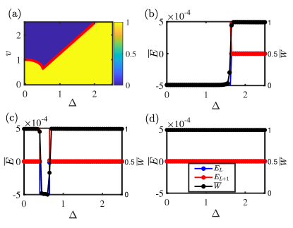
Figure 2: (Color online) (a) Disorder-averaged winding number $\overline{W}$ as a function of the modulation strength $\Delta$ and the amplitude of the intracell hopping $v$ with $L=200$ and $N_{c}=100$ disorder realizations. The colorbar shows the value of disorder-averaged winding number $\overline{W}$. Two red dot lines represent the analytic critical lines Eqs. (8a) and (8b) for the divergence of the localization length $\lambda$ of the $L$-th eigenstate. (b-d)Two disorder-averaged energies $\overline{E}_{L}$ and $\overline{E}_{L+1}$ in the center of the spectrum, and the disorder-averaged winding number $\overline{W}$ as a function of the modulation strength $\Delta$ under OBCs with $v=2$(b), $v=0.8$(c) and $v=0.2$(d), respectively.

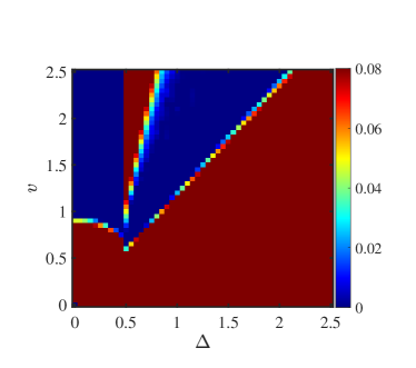
Figure 3: (Color online) $\lambda_{L}^{-1}$ of the $L$-th eigenstate as a function of $v$ and $\Delta$ for $L=600$ and $N_{c}=100$ disorder realization. The colorbar shows the value of $\lambda_{L}^{-1}$.

One can apply the open-bulk winding number to obtain the topological phase diagram of the SSH model without translational symmetry. For a given modulation configuration, we can solve the Hamiltonian as $H|\psi^{n}\rangle=E_{n}|\psi^{n}\rangle$ with $E_{n}\geq 0$ and $|\tilde{\psi}^{n}\rangle=S|\psi^{n}\rangle$ corresponding to an eigenvector with $-E_{n}$, where the entries of the chiral operator are $S_{m\alpha,h\delta}=\delta_{mh}(\sigma_{z})_{\alpha\delta}$ with $m,h$ referring to the unit cell and $\alpha,\delta$ to the sublattice. We introduce an open-boundary $Q$ matrix given by

$$Q=\sum_{n}^{\prime}\left(|\psi^{n}\rangle\langle\psi^{n}|-|\tilde{\psi}^{n}\rangle\langle\tilde{\psi}^{n}|\right),$$ (4)

where $\sum\limits_{n}^{\prime}$ is the sum over the eigenstates in the bulk spectrum without the edge modes. The open-bulk winding number in real space is defined as Song2019PRL

$$W_{c}=\frac{1}{2L^{\prime}}\mathrm{Tr}^{\prime}(SQ[Q,X]).$$ (5)

Here, $X$ is the coordinate operator, namely $X_{m\alpha,h\delta}=m\delta_{mh}\delta_{\alpha\delta}$. The length of the system $L$ can be divided into three intervals with length $l$, $L^{\prime}$ and $l$, i.e., $L=L^{\prime}+2l$. The symbol $\mathrm{Tr}^{\prime}$ represents the trace over the middle interval of length $L^{\prime}$. Furthermore, we define the disorder-averaged winding number $\overline{W}=1/N_{c}\sum_{c=1}^{N_{c}}W_{c}$ with the configuration number $N_{c}$.

Figure 2(a) shows the topological phase diagram on the $v$-$\Delta$ plane obtained by numerically computing $\overline{W}$. As shown in Figure 2(a), one can divide the topological phase diagram into three regions, i.e., $v>1$, $0.6<v<1$, and $v<0.6$. For the $v>1$ region, the clean case presents topologically trivial features. When the modulation amplitude goes beyond a finite value, the system enters into the TAI phase, which is robust against the modulation. As shown in Fig. 2(b) with $v=2$, when $\Delta>1.6$, the disorder-averaged zero modes are induced by the moderate modulations, accompanied by the jump of $\overline{W}$ from 0 to 1. Moreover, the quasi-periodic modulation would not destroy the TAI phase. For $v\in(0.6,1)$, the system undergoes topological transitions among nontrivial-trivial-nontrivial regions as $\Delta$ increases. A clear picture can be obtained by the average winding number and the two disorder-averaged zero modes as a function of $\Delta$ for $v=0.8$, as shown in Fig. 2(c). For small $\Delta$, $\overline{W}=1$ and $\overline{E}_{L}=\overline{E}_{L+1}=0$, which is topologically nontrivial. For $\Delta\in(0.45,0.65)$, the average winding number $\overline{W}$ jumps to $0$ and the values of the corresponding $\overline{E}_{L}$ and $\overline{E}_{L+1}$ break into nonzero pairs. It indicates that the modulation destroys the nontrivial topology. A modulation-induced topology emerge again in the $\Delta>0.65$ region, which known as RTAI. Here, $\overline{E}_{n}=1/N_{c}\sum_{c=1}^{N_{c}}E_{n}^{c}$ with $E_{n}^{c}$ being the $n$-th eigenenergy for a given modulation configuration. The TAI and RTAI phases induced by the quasi-periodic modulations in the SSH model are robust against the disorder in our system. When $v<0.6$, the SSH model is topologically nontrivial, and this feature is robust against the quasi-periodic modulations. It implies that in this regime, an arbitrary quasi-periodic modulation amplitude $\Delta$ will not break the nontrivial topology of the system. For the case $v=0.2$, with the increase of $\Delta$, $\overline{W}$ keeps unit, and the two disorder-averaged zero modes $\overline{E}_{L}$ and $\overline{E}_{L+1}$ are kept to zero, as shown in Fig. 2(b).

According to Figs. 2(b)-(d), in the topologically nontrivial regime, we find the emergence of the zero modes is always accompanied by a nonzero average winding number $\overline{W}=1$, and the zero modes are localized at the edges with a finite localization length. However, when the system enters the trivial regime, these edge modes vanish and bulk states emerge with the divergence of the localization length Hughes2014 ; Longhi2020 . Therefore, one can analytically obtain the topological phase diagram by studying the localization length of the zero modes. The Schrödinger equation of the SSH model Eq. (1) with zero modes, $H\psi=0$, is given by:

$$w_{m}\psi_{m,B}+v_{m+1}\psi_{m+1,B} = 0$$

$$v_{m}\psi_{m,A}+w_{m}\psi_{m+1,A} = 0,$$ (6)

where $\psi_{m,A}$($\psi_{m,B}$) is the probability amplitude of the zero mode on the sublattice site $A(B)$ in the $m$-th lattice cell. By solving the coupled equations, one can obtain $\psi_{n+1,A}=(-1)^{n}\prod_{m=1}^{n}(v_{m}/w_{m})\psi_{1,A}$, leading to the localization length $\lambda$ of the zero modes given by Longhi2020 ; J.K.2016

$$\lambda^{-1} = -\lim_{L\to\infty}\frac{1}{L}\ln\left|\frac{\psi_{L+1,A}}{\psi_{1,A}}\right|$$ (7)

$$= \lim_{L\to\infty}\frac{1}{L}\left|\sum_{m=1}^{L}\ln{\frac{|1+\gamma\Delta\cos(2\pi\beta m)|}{|v+\Delta\cos(2\pi\beta m)|}}\right|.$$

The divergence of the localization length $\lambda$, i.e., $\lambda^{-1}\to 0$, gives the topological phase transition boundaries (see Appendix A for the derivation)

$${{1+\sqrt{1-\gamma^{2}\Delta^{2}}}}= {v+\sqrt{v^{2}-\Delta^{2}}} \Delta<\frac{1}{\gamma}\ {\rm{and}}\ \Delta<v$$ (8a)

$$\Delta= \frac{2\gamma}{1+\gamma^{2}}v {\frac{1}{\gamma}<\Delta<v.}$$ (8b)

The analytic results are shown in Fig. 2(a) marked by the red solid lines, which match our numerical results. One can numerically calculate the value of $\lambda^{-1}$ for the $L$-th eigenstate, which is also known as the Lyapunov exponent, by Hughes2014 ; WZH2022PRB ; MacKinnon1983

$$\lambda^{-1} = \lim_{L\to\infty}\frac{1}{L}\ln||T||,$$ (9)

where $\|T\|$ denotes the norm of the total transfer matrix $T=\prod_{m=2}^{L}T_{m}T_{1}$ with

$$T_{m} = \left[\begin{array}[]{cc}\frac{E_{L}^{2}-v_{m}^{2}-w_{m-1}^{2}}{v_{m}w_{m}}&-\frac{w_{m-1}v_{m-1}}{v_{m}w_{m}}\\ 1&0\\ \end{array}\right],$$ (12)

and

$$T_{1} = \left[\begin{array}[]{cc}\frac{E_{L}^{2}-v_{m}^{2}}{v_{m}w_{m}}&-1\\ 1&0\\ \end{array}\right].$$ (15)

Figure. 3 shows the $\lambda_{L}^{-1}$ for the $L$th eigenstate as a function of $v$ and $\Delta$ with $2L=1200$ and $N_{c}=100$. The diverging lines indeed match our topological phase boundaries in Fig. 2(a).

IV Localization phase diagram and Reentrant localization transition

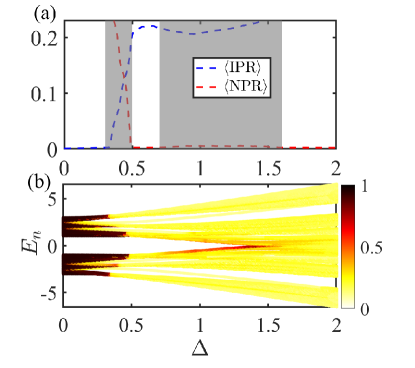
Figure 4: (Color online) (a) $\langle\rm{IPR}\rangle$ (blue dashed line) and $\langle\rm{NPR}\rangle$ (red dashed line) as a function of the modulation strength $\Delta$, showing the reentrant localization transition. The shaded regions represent the intermediate regimes with ME. (b) The fractal dimension $\mathrm{\Gamma}_{n}$ of different eigenstates as a function of the corresponding eigenvalues and the modulation strength $\Delta$. The colorbar indicates the magnitude of $\mathrm{\Gamma}_{n}$. Other parameters: $\phi=0$, $v=2$ and $L=1000$.

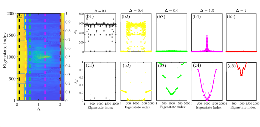
Figure 5: (Color online)(a)The fractal dimension $\mathrm{\Gamma}_{n}$ associated with the eigenstate indices as a function of $\Delta$. The vertical dashed lines of different colors correspond to $\Delta=0.1,0.4,0.6,1.3$ and $2$. And the corresponding distributions of the $\sigma_{n}$ and $\lambda_{n}^{-1}$ as a function of the eigenstate index are shown in (b1)-(b5) and (c1)-(c5), respectively. Other parameters: $\beta=(\sqrt{5}-1)/2$, $\phi=0$, $v=2$ and $L=1000$.

To obtain the localization properties of the system, we rely on the inverse participation ratio $(\rm{IPR})$ and the normalized participation ratio $(\rm{NPR})$, which are defined respectively as

$$\mathrm{IPR}_{n} = \sum_{m=1}^{L}\sum_{\alpha}|\psi_{m,\alpha}^{n}|^{4},$$

$$\mathrm{NPR}_{n} = \left(2L\sum_{m=1}^{L}\sum_{\alpha}|\psi_{m,\alpha}^{n}|^{4}\right)^{-1},$$ (16)

where $\psi_{m,\alpha}^{n}$ is the probability amplitude of the $n$-th eigenstate on the sublattice site $\alpha$($\alpha=A\$or$\ B$) in the $m$-th unit cell. It is known that ${\mathrm{IPR}_{n}}$ tends to zeros(nonzero) and ${\mathrm{NPR}_{n}}$ is nonzero(zero) for the extended(localized) phases in the thermodynamic limit. In order to see the localization transition point more clearly, we average the ${\mathrm{IPR}_{n}}$ and ${\mathrm{NPR}_{n}}$ over all eigenstates to obtain $\langle\rm{IPR}\rangle$ and $\langle\rm{NPR}\rangle$. In Fig. 4(a), we show $\langle\rm{IPR}\rangle$ and $\langle\rm{NPR}\rangle$ as a function of the modulation amplitude $\Delta$ under OBCs for $v=2$ and $\phi=0$, which are marked by the blue and red dashed lines, respectively. In the clean case, the system is in the extended phase characterized by $\langle\rm{IPR}\rangle=0$ and $\langle\rm{NPR}\rangle\neq 0$. As $\Delta$ increases, the system enters into the first intermediate phase marked by the shaded region for $0.3<\Delta<0.5$, accompanied by the nonzero values of $\langle\rm{IPR}\rangle$ and $\langle\rm{NPR}\rangle$. It implies that the extended and localized eigenstates coexist in this region. In the region $\Delta\in(0.5,0.7)$, all the states become localized with $\langle\rm{IPR}\rangle\neq 0$ and $\langle\rm{NPR}\rangle=0$. With the further increase of $\Delta$, the values of the $\langle\rm{IPR}\rangle$ and $\langle\rm{NPR}\rangle$ are again restored to finite marked by the second shaded region, which indicates the system enters into the second intermediate phase hosting the ME. When $\Delta>1.6$, all eigenstates localized again. According to our calculation, the intermediate phases in this system are localized in two separate regions $\Delta\in(0.3,0.5)$ and $(0.7,1.6)$, a clear sign of the reentrant localization phenomenon.

The reentrant localization feature can be detected in the energy spectrum encoded with the corresponding fractal dimension $\mathrm{\Gamma}_{n}$, which is defined as:

$$\mathrm{\Gamma}_{n} = -\lim_{L\to\infty}\frac{\ln{\mathrm{IPR}_{n}}}{\ln{(2L)}}.$$ (17)

In the large $L$ limit, $\Gamma_{n}\to 1$ for extended states, $\Gamma_{n}\to 0$ for localized states, and $0<\Gamma_{n}<1$ for the critical ones Wang2020PRL2 . Fig. 4(b) shows $\mathrm{\Gamma}_{n}$ as a function of all the eigenenergies and $\Delta$ for $v=2$ and $L=1000$ under OBCs. The regions with black (yellow) color for all states indicate the extended (localized) phases at a weak (strong) modulation, and two intermediate phases in $0.3<\Delta<0.5$ and $0.7<\Delta<1.6$ with the ME. It clearly shows that the system undergoes two intermediate regions.

In order to further distinguish the localization states from the extended ones, we can also apply the standard deviations of the coordinates $\sigma_{n}$ and the localization length $\lambda_{n}$ of eigenstates with the eigenvalue $E_{n}$, respectively. The standard deviations of the eigenstate coordinates $\sigma_{n}$ are given by Yicaizhang2022

$$\sigma_{n} = \sqrt{\sum\limits_{i=1}^{2L}\left(i-\overline{i}\right)^{2}\left|\psi^{n}(i)\right|^{2},}$$ (18)

where $i$ is the lattice coordinate and $\overline{i}=\sum\limits_{i=1}^{2L}i\left|\psi^{n}(i)\right|^{2}$ is the position of the center of mass. $\sigma_{n}$ contains the information about the spatial distribution of the eigenstates. While $\sigma_{n}$ is small for a localized state and larger for the extended state, the standard deviations of the critical states are in between of them and exhibit fluctuation. The inverse of the localization length $\lambda^{-1}_{n}$ for the $n$-th eigenstate, measures the average growth rate of the wave function, and can be calculated by Eq.(9). The case $\lambda^{-1}_{n}>0$ corresponds to a localized state, and a delocalized state is characterized by $\lambda^{-1}_{n}=0$ yanxialiu2 . Figure. 5(a) shows the fractal dimensions $\Gamma_{n}$ associated to eigenstate indices as a function of $\Delta$. It can be seen that some eigenstates are localized and the rest are delocalized in $0.3<\Delta<0.5$ and $0.7<\Delta<1.6$ regions, where both $\langle\rm{IPR}\rangle$ and $\langle\rm{NPR}\rangle$ are finite. We discuss the localization features in different regimes by taking $\Delta=0.1,0.4,0.6,1.3$ and $2$ as examples, which are marked by dashed lines with different colors shown in Fig. 5(a). And the corresponding distributions of the $\sigma_{n}$ and $\lambda^{-1}_{n}$ as a function of the eigenstate indices $n$ are shown in Fig. 5(b1)-(b5) and 5(c1)-(c5), respectively. For $\Delta=0.1$, all the eigenstates are extended. As shown in Fig. 5(b1) and (c1), the standard deviations
of almost all eigenstates $\sigma_{n}$ are stabilized at a large value and the corresponding values of the $\lambda^{-1}_{n}$ approach zero. When $\Delta=0.4$, $\lambda^{-1}_{n}\to 0$ and the standard deviations of the eigenstates $\sigma_{n}$ display extended behaviors in the band-center region, as shown in the Fig. 5(b2) and (c2). And in the band-edge region, $\lambda^{-1}_{n}>0$ and $\sigma_{n}$ is very small corresponding to the localized properties. The coexistence of delocalized and localized states indicates the system is localized in the intermediate phase hosting ME. Further increasing $\Delta$ to $0.6$, the system is localized in the localization regime, where the standard deviations of all the eigenstates are stabilized at very small values and $\lambda^{-1}_{n}$ of all the eigenstates take finite values, as shown in the Fig. 5(b3) and (c3). In Fig. 5(b4) and (c4), we find that the values of $\sigma_{n}$ of some of eigenstates in the band-center region exhibit a relatively large fluctuation and the corresponding values of $\lambda^{-1}_{n}$ tend to zero, implying that some eigenstates in the band-center region reenter into the delocalization regime for $\Delta=1.3$. When the modulation strength is large enough, such as $\Delta=2$ in Fig. 5(b5) and (c5), the system is recovered into a fully localized regime. As $\Delta$ increases, the band of the spectrum shows a sequential transition between extended-intermediate-localized-intermediate-localized regions. The numerical results clearly show that the existence of the second intermediate region and the ME.

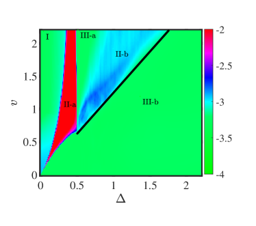
Figure 6: (Color online) The localization phase diagram in the $v-\Delta$ plane obtained using the values of $\overline{\eta}$ for $L=1000$. The regions for extended, intermediate and localized phases are denoted by I , II-a(II-b) , and III-a(III-b) , respectively. The black lines represent the analytic critical lines Eq. (8b) for topological transition point. The colorbar represents the values of $\overline{\eta}$. All data in this figure are averaged over 100 disorder realizations.

To obtain the full localization phase diagram on the $\Delta-v$ plane, we define a disorder-average quantity $\overline{\eta}=1/N_{c}\sum_{c=1}^{N_{c}}\eta_{c}$ xiaoli , which can clearly distinguish the intermediate region from the extended and localized regions in the phase diagram. Here,

$$\eta_{c}=\log_{10}\left[\langle\rm{IPR}\rangle\langle\rm{NPR}\rangle\right].$$ (19)

As shown in Fig. 6, there are three phases in this system: I, II-a(II-b), and III-a(III-b) corresponding to the extended, intermediate and localized phases, respectively. For $v<0.6$, only one intermediate region exists in a finite range of $\Delta$. While for $v>0.8$, the phase diagram clearly shows two intermediate regions, marked in red and blue, separated by phase III-a.

Comparing the localization phase diagram Fig. 6 with the topological phase diagram Fig. 2(a), one can see that the reentrant localization transition almost coincides with the TAI and RTAI phase transitions. The analytical line Eq.(8b) corresponding to the TAI and RTAI transitions is replotted in solid line in Fig. 6, which fits pretty well with the reentrant localization transition boundary. In phase III-a, where all the states are localized, the system is topologically trivial without localized edge modes. It means that the states near the zero energy value are trivial bulk with the localized property. However, for sufficiently large $\Delta$, the system enters into the TAI or RTAI regime induced by $\Delta$. In this regime, the zero energy states become localized edge ones. In phase II-b, the localized bulk modes in the band-center region should undergo a delocalized process evolving into the localized edge modes Goblot2020 ; ZZhai2021 . Thus, the emergence of the reentrant localisation transition accompanies the TAI transition in our case.

V Dynamical Detection

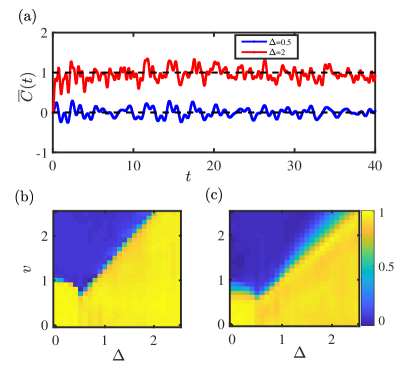
Figure 7: (Color online) (a) Dynamics of $\overline{C}(t)$ with $L=100$, $v=2$ and $N_{c}=100$ disorder realizations for $\Delta=0.5$ and $\Delta=2$, respectively. $\langle\overline{C}\rangle$ as a function of the modulation strength $\Delta$ and the amplitude of the intracell hopping $v$ for $L=100$ (b) and $L=10$ (c) under $N_{c}=100$ disorder realizations. The colorbar indicates the magnitude of the $\langle\overline{C}\rangle$.

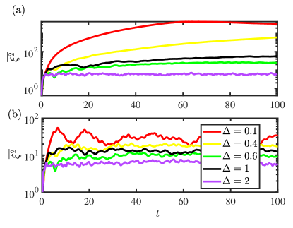
Figure 8: (Color online) The mean-square displacement $\overline{\xi^{2}}(t)$ as a function of the time $t$ for $\Delta=0.1,0.4,0.6,1$ and $2$ in $L=100$(a) and $L=10$(b) under $N_{c}=100$ disorder realizations. Other parameters: $v=2$ and $\beta=\frac{\sqrt{5}-1}{2}$.

To realize our model, one can implement the 1D momentum lattice technique in cold atom experiments. Discrete momentum states can be coupled by pairs of Bragg lasers. By engineering the frequencies $\omega_{h}$ of the multicomponent Bragg lasers, the counter-propagating laser pairs drive a series of two-photon Bragg resonance transitions, which couple the adjacent momentum states separated by $2\hbar k$, where $k$ is the wave number. The off-diagonal modulation, in our case, can be individually tuned by adjusting the amplitude of the Bragg beam with frequency $\omega_{h}$ for the function $v_{m}$ and $w_{m}$. Here, $\omega_{h}$ is tuned to the two-photon resonance between the corresponding momentum states via an acousto-optic modulator. In current experiments, by using ⁸⁷Rb or ¹³³Cs atoms, the typical system size is $\sim 20$ sites. In the following, we choose $L=10$ for our numerical simulation. We also calculate the dynamical detection with a large system size ($L=100$) for comparison.

To dynamically investigate the topological properties of the quasi-periodic modulated SSH model, one can measure the mean chiral displacement Meier2018 ; Scherg2018 . We define the single-shot expectation value of the mean chiral displacement operator in a given modulation configuration as Meier2018 ; SNL2022

$$C_{c}(t)=2\langle\psi(t)|SX^{\prime}|\psi(t)\rangle,$$ (20)

where $|\psi(t)\rangle=e^{-iHt}|\psi(0)\rangle$ is the time-evolved wave function. $|\psi(0)\rangle$ is the initial wave function and the entire atomic population is initially localized at a single central site. Here, $X^{\prime}=X-(L/2+1)$ Meier2018 . $L$ is even number. The dynamics of the disorder-average mean chiral displacement $\overline{C}(t)=1/N_{c}\sum_{c=1}^{N_{c}}C_{c}(t)$ generally exhibit a transient, oscillatory behavior. To eliminate the oscillation, we take their time-average $\langle\overline{C}\rangle$, which converges to the corresponding winding number $\overline{W}$ Meier2018 ; SNL2022 . Figure 7(a) displays the dynamics of $\overline{C}(t)$ for both weak ($\Delta=0.5$) and strong ($\Delta=2$) modulations for $v=2$ with $L=100$. We can see that the dynamics of $\overline{C}(t)$ show transient and oscillatory processes and eventually converge to their corresponding $\overline{W}$ (marked by the black dashed lines, respectively) in long time limits. Moreover, we can obtain the topological phase diagram through the $\langle\overline{C}\rangle$ in the $v-\Delta$ plane shown in Figs. 7(b) with $L=100$ and (c) with $L=10$. By comparing the dynamical evolution behaviors of different system sizes, one can find that the mean chiral displacement $\langle\overline{C}\rangle$ can effectively characterize the topological properties even in a small-sized system.

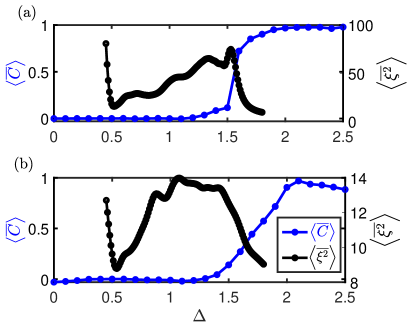
Figure 9: (Color online) The mean square displacement $\left<\overline{\xi^{2}}\right>$ (black line) and the mean chiral displacement $\left<\overline{C}\right>$ (blue line) as a function of the modulation strength $\Delta$ with $L=100$(a) and $L=10$(b), respectively. Other parameters: $v=2$ and $\beta=\frac{\sqrt{5}-1}{2}$. All data in this figure are averaged over $100$ disorder realizations.

To characterize the signatures of the multiple localization transitions, we can calculate the mean-square displacement for a given modulation realization defined as Padhan2022PRB ; Scherg2018 ; ZHXU2020

$$\xi^{2}_{c} = \sum_{i}\left(i-i_{0}\right)^{2}\left|\psi_{i}(t)\right|^{2},$$ (21)

where the entire atomic population is initially localized at the center of the lattice $i_{0}$. We can use the behavior of the disorder-averaged mean-square displacement $\overline{\xi^{2}}$ in the long-time evolution to verify the localization properties of the system Padhan2022PRB . Here $\overline{\xi^{2}}=1/N_{c}\sum_{c=1}^{N_{c}}\xi^{2}_{c}$. As shown in Fig. 8(a), $\overline{\xi^{2}}$ saturates to different values after a long time evolution with various $\Delta$ for $v=2$ and $L=100$, indicating multiple localization transitions. According to the localization phase diagram in Fig. 6, the system is in the extended, intermediate, localized, intermediate, and localized phases for $\Delta=0.1,0.4,0.6,1$ and $2$, respectively. The corresponding saturation values of $\overline{\xi^{2}}$ exhibit different features. For $\Delta=0.1$, the system is in the extended phase with the highest saturation values of $\overline{\xi^{2}}$. For $\Delta=0.4$ and $1$, the system is in the intermediate phase, and the saturation values of $\overline{\xi^{2}}$ are larger than those at $\Delta=0.6$ and $2$, where the system is in the localized phase. To examine the impact of size on the system, we also calculate $\overline{\xi^{2}}$ with different $\Delta$ for $L=10$, as shown in Fig. 8(b). It is evident that, even in the small size, the saturation value of $\overline{\xi^{2}}$ after a long evolution can still reflect the multiple localization transitions of the system.

To detect the topological transition associated with the localization transition in the expansion dynamics, we present a plot of the time-averaged mean-square displacement $\langle\overline{\xi^{2}}\rangle$ and $\langle\overline{C}\rangle$ as a function of $\Delta$ for $v=2$ with $L=100$ and $10$, shown in Fig. 9(a) and (b), respectively. According to the phase diagram in Fig. 6, the system is in the intermediate phase for $\Delta=0.45$ and $v=2$, with a correspondingly high value of $\langle\overline{\xi^{2}}\rangle$. Upon increasing $\Delta$, the system enters the localized phase with a sharp decrease of $\langle\overline{\xi^{2}}\rangle$. As $\Delta$ increases, the system reenters the intermediate phase, and the corresponding $\langle\overline{\xi^{2}}\rangle$ rapidly increases. However, for $\Delta>1.5$, $\langle\overline{\xi^{2}}\rangle$ decreases rapidly, indicating that all the states are localized once again. At the same time, the system entered the TAI region, as evidenced by a jump of $\langle\overline{C}\rangle$ from $0$ to $1$. These results suggest that reentrant localization occurs in association with the TAI transition. Comparison with the results in Fig. 9(b) reveals a similar transition process for a small sized system $L=10$. The above analyses indicate that expansion dynamics can be used to detect the coincidence of the TAI and reentrant localization transitions.

VI Summary

In this study, we investigated the topological and localization properties of a generalized SSH model with off-diagonal quasi-periodic modulations. Contrary to the conventional case where sufficiently strong disorder always destroys the topologically nontrivial properties, a suitable choice of disorder structure can induce the emergence of the robust topological phase in the case of sufficiently strong disorder. In particular, we found that the off-diagonal quasi-periodic modulations can induce the emergence of the stable TAI and RTAI phases. Furthermore, we investigated the localization properties of our system. Comparing the topological phase diagram and the localization transition, we find that a reentrant localization transition accompanies the TAI/RTAI transition. It implies that topology properties are crucial in establishing the reentrant localization transition. Finally, we employed wave-packet dynamics in different parameter regimes to characterize and detect the TAI and reentrant localization. Our findings can be simulated in cold atom systems by applying the momentum lattice technology.

Appendix A: Derivation of the analytical expression for the topological phase transition point

In this Appendix, we present a detailed derivation of the expression of Eqs. (8a) and (8b) in the main text. First, the Eq. (7) can be simplified as follows

$$\small\lambda^{-1} = \lim_{L\to\infty}\frac{1}{L}\Bigg{|}\sum_{m=1}^{L}\big{[}\ln{|1+\gamma\Delta\cos(2\pi\beta m)|}$$ (A1)

$$- \ln{|v+\Delta\cos(2\pi\beta m)|}\big{]}\Bigg{|}.$$

According to Weyl’s equidistribution theorem Weyl1916 ; Choe1993 , we can use the ensemble average to evaluate the above expression

$$\small\lambda^{-1} = \left|\frac{1}{2\pi}\int^{\pi}_{-\pi}(\ln{|1+\gamma{\Delta}\cos q|}-\ln{|v+{\Delta}\cos q|})dq\right|$$ (A2)

$$= \Big{|}\frac{1}{2\pi}\int^{\pi}_{-\pi}\ln{|1+\gamma{\Delta}\cos q|}dq$$

$$- \frac{1}{2\pi}\int^{\pi}_{-\pi}\ln{|v+{\Delta}\cos q|}dq\Big{|}.$$

The first part of the integration of the Eq.(A2) can be performed straightforwardly as

$$\frac{1}{2\pi}\int^{\pi}_{-\pi}\ln{|1+\gamma{\Delta}\cos q|}dq=\begin{cases}\ln{\frac{1+\sqrt{1-\gamma^{2}\Delta^{2}}}{2}}\quad&1>\gamma\Delta\\ \ln{\frac{\gamma\Delta}{2}}\quad&1<\gamma\Delta\\ \end{cases}$$ (A3)

and the second part is

$$\small\frac{1}{2\pi}\int^{\pi}_{-\pi}\ln{|v+{\Delta}\cos q|}dq=\begin{cases}\ln{\frac{v+\sqrt{v^{2}-\Delta^{2}}}{2}}\quad&v>\Delta,\\ \ln{\frac{\Delta}{2}}\quad&v<\Delta.\\ \end{cases}$$ (A4)

Combining the results (A3) and (A4), there are four possible situations:

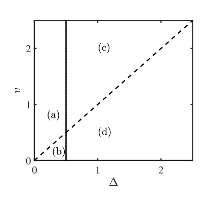
Figure A1: (Color online) The four regions: (a), (b), (c) and (d) in the $v-\Delta$ plane.

(a)For $\Delta<\frac{1}{\gamma}$ and $\Delta<v$, we have

$$\lambda^{-1}=\left|\ln{\frac{{1+\sqrt{1-\gamma^{2}\Delta^{2}}}}{v+\sqrt{v^{2}-\Delta^{2}}}}\right|.$$ (A5)

(b)For $\Delta<\frac{1}{\gamma}$ and $\Delta>v$, we have

$$\lambda^{-1}=\left|\ln{\frac{{1+\sqrt{1-\gamma^{2}\Delta^{2}}}}{\Delta}}\right|.$$ (A6)

(c)For $\Delta>\frac{1}{\gamma}$ and $\Delta<v$, we have

$$\lambda^{-1}=\left|\ln{\frac{\gamma\Delta}{v+\sqrt{v^{2}-\Delta^{2}}}}\right|.$$ (A7)

(d)For $\Delta>\frac{1}{\gamma}$ and $\Delta>v$, we have

$$\small\lambda^{-1}=\left|\ln\gamma\right|.$$ (A8)

According to the above results, the $v-\Delta$ plane can be divided into four regions by two lines $v=\Delta$ and $\Delta=\frac{1}{\gamma}$ (Here, we consider $\gamma>1$), as shown in Fig. A1. $\lambda^{-1}=0$ is the topological phase transition point. Since $\gamma>1$, we can get $\left|\ln\gamma\right|>0$. No topological phase transition exist in region (d). For case (b) ($v<\Delta<\frac{1}{\gamma}$), we have

$${{1+\sqrt{1-\gamma^{2}\Delta^{2}}}} = \Delta,$$ (A9)

which contradicts the preliminary condition ($\Delta<\frac{1}{\gamma}$). Hence, the case (b) is also excluded. Combining the results (A5) and (A7), we obtain

$${{1+\sqrt{1-\gamma^{2}\Delta^{2}}}}={v+\sqrt{v^{2}-\Delta^{2}}}\ \Delta<\frac{1}{\gamma}\ {\rm{and}}\ \Delta<v,$$ (A10)

and

$${\gamma\Delta} ={v+\sqrt{v^{2}-\Delta^{2}}}\ \frac{1}{\gamma}<\Delta<v.$$ (A11)

Here, $\Delta$ and $v$ are positive numbers. The Eq. (A11) can be further simplified as

$$\Delta =\frac{2\gamma}{1+\gamma^{2}}v.$$ (A12)

Combined with the above results, we obtain the topological transition boundary Eqs. (8a) and (8b) in the main text.

- (1) P. W. Anderson, Phys. Rev. 109, 1492 (1958).
- (2) P. A. Lee and T. V. Ramakrishnan, Rev. Mod. Phys. 57, 287 (1985).
- (3) J. Billy, V. Josse, Z. Zuo, A. Bernard, B. Hambrecht, P. Lugan, D. Clément, L. Sanchez-Palencia, P. Bouyer, and A. Aspect, Nature (London) 453, 891 (2008).
- (4) G. Roati, C. D’Errico, L. Fallani, M. Fattori, C. Fort, M. Zaccanti, G. Modugno, M. Modugno, and M. Inguscio, Nature (London) 453, 895 (2008).
- (5) A. A. Chabanov, M. Stoytchev, and A. Z. Genack, Nature (London) 404, 850 (2000).
- (6) P. Pradhan and S. Sridhar, Phys. Rev. Lett. 85, 2360 (2000).
- (7) Y. Lahini, R. Pugatch, F. Pozzi, M. Sorel, R. Morandotti, N. Davidson, and Y. Silberberg, Phys. Rev. Lett. 103, 013901 (2009).
- (8) N. Mott, J. Phys. C 20, 3075 (1987).
- (9) S. Aubry and G. André, Ann. Isr. Phys. Soc. 3, 133 (1980).
- (10) P. G. Harper, Proc. Phys. Soc. London Sect. A 68, 874 (1955).
- (11) S. Longhi, Phys. Rev. Lett. 122, 237601 (2019).
- (12) S. Longhi, Phys. Rev. B 100, 125157 (2019).
- (13) Y. E. Kraus, Y. Lahini, Z. Ringel, M. Verbin, and O. Zilberberg, Phys. Rev. Lett. 109, 106402 (2012).
- (14) M. Segev, Y. Silberberg, and D. N. Christodoulides, Nat. Photonics 7, 197 (2013).
- (15) J. Biddle and S. Das Sarma, Phys. Rev. Lett. 104, 070601 (2010).
- (16) S. Ganeshan, J. H. Pixley, and S. Das Sarma, Phys. Rev. Lett. 114, 146601 (2015).
- (17) Y. Wang, L. Zhang, W. Sun, T.-F. J. Poon, and X.-J. Liu, Phys. Rev. B 106, L140203 (2022).
- (18) Xin-Chi Zhou, Yongjian Wang, Ting-Fung Jeffrey Poon, Qi Zhou, and Xiong-Jun Liu,arXiv:2212.14285 (2022).
- (19) T. Liu, X. Xia, S. Longhi, and L. Sanchez-Palencia, Sci-Post Phys. 12, 027 (2022).
- (20) N. Roy and A. Sharma, Phys. Rev. B 103, 075124 (2021).
- (21) A. Ahmed, N. Roy, and A. Sharma, Phys. Rev. B 104, 155137 (2021).
- (22) A. Ahmed, A. Ramachandran, I. M. Khaymovich, and A. Sharma, Phys. Rev. B 106, 205119 (2022).
- (23) T. Liu, S. Cheng, H. Guo, and G. Xianlong, Phys. Rev. B 103, 104203 (2021).
- (24) J. Wang, X.-J. Liu, G. Xianlong, and H. Hu, Phys. Rev. B 93, 104504 (2016).
- (25) V. Goblot, A. Štrkalj, N. Pernet, J. L. Lado, C. Dorow, A. Lemaître, L. Le Gratiet, A. Harouri, I. Sagnes, S. Ravets, A. Amo, J. Bloch and O. Zilberberg, Nat. Phys. 16, 832-836 (2020).
- (26) L. J. Zhai, G. Y. Huang, S. Yin, Phys. Rev. B. 104, 014202 (2021).
- (27) S. Roy, T. Mishra, B. Tanatar, and S. Basu, Phys. Rev. Lett. 126, 106803 (2021).
- (28) A. Padhan, M. K. Giri, S. Mondal and T. Mishra, Phys. Rev. B 105, L220201 (2022).
- (29) Z.-W. Zuo and D. Kang, Phys. Rev. A 106, 013305 (2022).
- (30) S. Aditya, K. Sengupta, and D. Sen, Phys. Rev. B 107, 035402 (2023).
- (31) S. Roy, S. Chattopadhyay, T. Mishra, and S. Basu, Phys. Rev. B 105, 214203 (2022).
- (32) C. Wu, J. Fan, G. Chen, and S. Jia, New J. Phys. 23, 123048 (2021).
- (33) X.-P. Jiang, Y. Qiao, and J.-P. Cao, Chin. Phys. B 30, 097202 (2021).
- (34) L. Zhou and W. Han, Phys. Rev. B 106, 054307 (2022).
- (35) W. Han and L. Zhou, Phys. Rev. B 105, 054204 (2022).
- (36) H. Wang, X. Zheng, J. Chen, L. Xiao, S. Jia, and L. Zhang, Phys. Rev. B 107, 075128 (2023).
- (37) S. Nakajima, N. Takei, K. Sakuma, Y. Kuno, P. Marra, and Y. Takahashi, Nat. Phys. 17, 844 (2021).
- (38) D. J. Thouless, M. Kohmoto, M. P. Nightingale, and M. den Nijs, Phys. Rev. Lett. 49, 405 (1982).
- (39) M. Z. Hasan and C. L. Kane, Rev. Mod. Phys. 82, 3045 (2010).
- (40) X.-L. Qi and S.-C. Zhang, Rev. Mod. Phys. 83, 1057 (2011).
- (41) A. Bansil, H. Lin, and T. Das, Rev. Mod. Phys. 88, 021004 (2016).
- (42) C. K. Chiu, J. C. Y. Teo, A. P. Schnyder, and S. Ryu, Rev. Mod. Phys. 88, 035005 (2016).
- (43) N. P. Armitage, E. J. Mele, and A. Vishwanath, Rev. Mod. Phys. 90, 015001 (2018).
- (44) W. P. Su, J. R. Schrieffer, and A. J. Heeger, Phys. Rev. Lett. 42, 1698 (1979).
- (45) F. Song, S. Yao, and Z. Wang, Phys. Rev. Lett. 123, 246801 (2019).
- (46) Z. Xu, R. Zhang, S. Chen, L. Fu, Y. Zhang, Phys. Rev. A 101, 013635 (2020).
- (47) T. Xiao, D. Xie, Z. Dong, T. Chen, W. Yi, and B. Yan, Sci. Bull. 66, 2175 (2021).
- (48) E. Prodan, T. L. Hughes, and B. A. Bernevig, Phys. Rev. Lett. 105, 115501 (2010).
- (49) X. Cai, L.-J. Lang, S. Chen, and Y. Wang, Phys. Rev. Lett. 110, 176403 (2013).
- (50) J. Li, R.-L. Chu, J. K. Jain, and S.-Q. Shen, Phys. Rev. Lett. 102, 136806 (2009).
- (51) C. W. Groth, M. Wimmer, A. R. Akhmerov, J. Tworzydlo, and C. W. J. Beenakker, Phys. Rev. Lett. 103, 196805 (2009).
- (52) H.-M. Guo, G. Rosenberg, G. Refael, and M. Franz, Phys. Rev. Lett. 105, 216601 (2010).
- (53) Y.-Y. Zhang, R.-L. Chu, F.-C. Zhang, and S.-Q. Shen, Phys. Rev. B 85, 035107 (2012).
- (54) J. Song, H. Liu, H. Jiang, Q.-F. Sun, and X. C. Xie, Phys. Rev. B 85, 195125 (2012).
- (55) A. Girschik, F. Libisch, and S. Rotter, Phys. Rev. B 88, 014201 (2013).
- (56) I. Mondragon-Shem, T. L. Hughes, J. Song, and E. Prodan, Phys. Rev. Lett. 113, 046802 (2014).
- (57) Z. Q. Zhang, B. L. Wu, J. Song, and H. Jiang, Phys. Rev. B 100, 184202 (2019).
- (58) D.-W. Zhang, L.-Z. Tang, L.-J. Lang, H. Yan, and S.-L. Zhu, Sci. China Phys. Mech. Astron. 63, 267062 (2020).
- (59) L.-Z. Tang, L.-F. Zhang, G.-Q. Zhang, and D.-W. Zhang, Phys. Rev. A 101, 063612 (2020).
- (60) J. Borchmann, A. Farrell, and T. Pereg-Barnea, Phys. Rev. B 93, 125133 (2016).
- (61) C.-B. Hua, R. Chen, D.-H. Xu, and B. Zhou, Phys. Rev. B 100, 205302 (2019).
- (62) G.-Q. Zhang, L.-Z. Tang, L.-F. Zhang, D.-W. Zhang, and S.-L. Zhu, Phys. Rev. B 104, L161118 (2021).
- (63) S. Velury, B. Bradlyn, and T. L. Hughes, Phys. Rev. B 103, 024205 (2021).
- (64) S. N. Liu, G. Q. Zhang, L. Z. Tang, and D. W. Zhang, Phys. Lett. A 431, 128004 (2022).
- (65) Y.-P. Wu, L.-Z. Tang, G.-Q. Zhang, D.-W. Zhang, Phys. Rev. A 106, L051301 (2022).
- (66) W.-J. Zhang, Y.-P. Wu, L.-Z. Tang, and G.-Q. Zhang, Commun. Theor. Phys. 74, 075702 (2022).
- (67) S. Stützer, Y. Plotnik, Y. Lumer, P. Titum, N. H. Lindner, M. Segev, M. C. Rechtsman, and A. Szameit, Nature (London) 560, 461 (2018).
- (68) G. G. Liu, Y Yang, X Ren, H. Xue, X Lin, Y. H. Hu, H. X. Sun, B Peng, P Zhou, Y. Chong, and B. Zhang, Phys. Rev. Lett. 125, 133603 (2020).
- (69) E. J. Meier, F. A. An, A. Dauphin, M. Maffei, P. Massignan, T. L. Hughes, and B. Gadway, Science 362, 929 (2018).
- (70) S. Longhi, Opt. Lett. 45, 4036 (2020).
- (71) L.-Z. Tang, S.-N. Liu, G.-Q. Zhang, and D.-W. Zhang, Phys. Rev. A 105, 063327 (2022).
- (72) Z.-H. Wang, F. Xu, L. Li, D.-H. Xu, and B. Wang, Phys. Rev. B 105, 024514 (2022).
- (73) A. MacKinnon and B. Kramer, Z. Phys. B 53, 1 (1983).
- (74) Y. Wang, L. Zhang, S. Niu, D. Yu, and X.-J. Liu, Phys. Rev. Lett. 125, 073204 (2020).
- (75) Y.-C. Zhang and Y.-Y. Zhang, Phys. Rev. B 105, 174206 (2022).
- (76) Y. Liu, Y. Wang, Z. Zheng, and S. Chen, , Phys. Rev. B 103, 134208 (2021).
- (77) X. Li and S. Dasl Sarma, Phys. Rev. B 101, 064203 (2020).
- (78) J. K. Asbóth, L. Oroszlány, and A. Pályi, A Short Course on Topological Insulators: Band Structure and Edge States in One and Two Dimensions (Springer International Publishing, Switzerland, 2016).
- (79) H. P. Lschen, S. Scherg, T. Kohlert, M. Schreiber, P. Bordia, X. Li, S. Das Sarma, and I. Bloch, Phys. Rev. Lett. 120, 160404 (2018).
- (80) Z. Xu, H. Huangfu, Y. Zhang, and S. Chen, New J. Phys. 22, 013036 (2020).
- (81) H. Weyl, Ueber die Gleichverteilung von Zahlen mod. Eins, Math. Ann. 77, 313 (1916).
- (82) G. H. Choe, Ergodicity and Irrational Rotations, Proc. Royal Irish Acad. A, 93A, 193 (1993).