Monolithic Algebraic Multigrid Preconditioners for the Stokes Equations

Abstract

In this paper, we investigate a novel monolithic algebraic multigrid solver for the discrete Stokes problem discretized with stable mixed finite elements. The algorithm is based on the use of the low-order $\boldsymbol{\mathbb{P}}_{1}\text{iso}\kern 1.0pt\boldsymbol{\mathbb{P}}_{2}/\mathbb{P}_{1}$ discretization as a preconditioner for a higher-order discretization, such as $\boldsymbol{\mathbb{P}}_{2}/\mathbb{P}_{1}$. Smoothed aggregation algebraic multigrid is used to construct independent coarsenings of the velocity and pressure fields for the low-order discretization, resulting in a purely algebraic preconditioner for the high-order discretization (i.e., using no geometric information). Furthermore, we incorporate a novel block LU factorization technique for Vanka patches, which balances computational efficiency with lower storage requirements. The effectiveness of the new method is verified for the $\boldsymbol{\mathbb{P}}_{2}/\mathbb{P}_{1}$ (Taylor-Hood) discretization in two and three dimensions on both structured and unstructured meshes. Similarly, the approach is shown to be effective when applied to the $\boldsymbol{\mathbb{P}}_{2}/\mathbb{P}_{1}^{disc}$ (Scott-Vogelius) discretization on 2D barycentrically refined meshes. This novel monolithic algebraic multigrid solver not only meets but frequently surpasses the performance of inexact Uzawa preconditioners, demonstrating the versatility and robust performance across a diverse spectrum of problem sets, even where inexact Uzawa preconditioners struggle to converge.

url]http://alexey-voronin.github.io/ url]https://www.math.mun.ca/ smaclachlan/

url]http://lukeo.cs.illinois.edu/

[1]organization=University of Illinois at Urbana-Champaign, addressline=Department of Computer Science, city=Urbana, state=IL, country=USA [2]organization=Memorial University of Newfoundland, addressline=Department of Mathematics and Statistics, city=St. John’s, state=NL, country=Canada [3]organization=Sandia National Laboratories, city=Livermore, state=CA, country=USA

1 Introduction

Differential equations and discrete problems with saddle-point structure arise in many scientific and engineering applications. Common examples are the incompressible Stokes and Navier-Stokes equations, where the incompressibility constraint leads to saddle-point problems at both the continuum level and for many common discretizations [1, 2]. Discretizations of these systems using stable finite-element pairs lead to a $2\times 2$ block structure in the resulting linear system, in which the lower-right diagonal block is a zero-matrix. The resulting indefiniteness in these matrices, along with the coupling between the two unknowns in the problem, prevents the straightforward application of standard geometric or algebraic multigrid methods. Several successful preconditioners for these systems are known in the literature, built on approximate block-factorization approaches [1, 3, 4] or monolithic geometric multigrid methods [5, 6, 7, 3, 8, 9]. While some algebraic multigrid algorithms have been proposed in the past [10, 11, 12, 13, 14], general-purpose algebraic multigrid methods that are successful for the numerical solution of a wide variety of discretizations of the Stokes equations are a recent (and still rare) development [15, 16, 17, 18]. In this work, we propose a robust and efficient algebraic multigrid method for the $\boldsymbol{\mathbb{P}}_{1}\text{iso}\kern 1.0pt\boldsymbol{\mathbb{P}}_{2}/\mathbb{P}_{1}$ discretization of the Stokes equations and show how it can be leveraged to develop an effective preconditioner for other discretizations, building on similar geometric multigrid methods in [19].

Monolithic geometric multigrid methods for these problems are well-known and date back to some of the earliest work on multigrid methods for finite-difference discretizations [20, 6, 7, 21]. In this work, and later work on finite-element discretizations [22, 23, 24, 25, 26, 3, 27], simultaneous geometric coarsening of velocity and pressure fields leads to coarse-grid operators that naturally retain stability on all grids of the hierarchy. This coarsening in combination with monolithic relaxation schemes, such as Vanka [6], Braess-Sarazin [8], or distributive [5] relaxation, has led to effective multigrid convergence for a wide variety of problems and discretizations. Despite the success and effectiveness of these methods, they are not without their challenges, particularly when considering their extension to algebraic multigrid approaches.

Two difficulties arise when attempting to extend these monolithic methods to algebraic multigrid approaches. First, it is difficult to construct independent algebraic coarsenings of the velocity and pressure fields that maintain algebraic properties of the fine-grid discretization (such as the relative number of velocity and pressure degrees of freedom) after Galerkin coarsening. As a result, it is possible that a stable discretization on the finest grid yields unstable discretizations on coarser grids in the algebraic multigrid hierarchy. Secondly, most inf-sup stable finite element discretizations of the Stokes equations rely on higher-order finite-element spaces (particularly for the discretized velocity), yielding discretization matrices that are far from the M-matrices for which classical AMG heuristics are known to work best [28, 29]. Consequently, even if stability problems are avoided, convergence of AMG-based solvers can deteriorate as the order of the discretization increases.

Many existing AMG approaches for the Stokes equations attempt to bypass coarsening issues by constraining AMG’s coarsening to loosely mimic properties of geometric multigrid. Specifically, it is possible to roughly maintain the ratio between the number of velocity degrees of freedom to the number of pressure degrees of freedom throughout the multigrid hierarchy by leveraging either geometric physical degree of freedom locations or element information [10, 11, 13, 12, 14]. While successful, this introduces additional heuristics that depend on both the fine-level discretization and the geometry of the mesh in the AMG process. Change-of-variable transformations have been used successfully to construct monolithic AMG preconditioners for saddle-point-type systems such as the Stokes equations [30, 15, 16, 17, 18]. These transformations convert the system into a similar one with a scalar elliptic operator in the bottom-right block, making it more suitable for classical multigrid’s unknown-based coarsening and point-wise smoothing. The method has been theoretically analyzed, showing a uniform bound on the spectral radius of the iteration matrix using a single step of damped Jacobi smoothing [15]. However, when applying these methods to Oseen problems using a two-level approach, it has been demonstrated that the use of more effective relaxation approaches such as Gauss-Seidel is necessary to achieve fast convergence [17]. Despite the successful extension of this approach to the multi-level regime [18], achieving robust convergence requires appropriate coarse-grid matrix-sparsification algorithms and the implementation of challenging-to-parallelize relaxation techniques such as Gauss-Seidel and successive over relaxation (SOR).

In this paper, we propose a new algebraic multigrid framework for the solution of the discretized Stokes equations, based on preconditioning higher-order discretizations by smoothed-aggregation AMG applied to the low-order $\boldsymbol{\mathbb{P}}_{1}\text{iso}\kern 1.0pt\boldsymbol{\mathbb{P}}_{2}/\mathbb{P}_{1}$ discretization. We make use of Vanka-style relaxation on both the original (high-order) discretization and on each level of the AMG hierarchy. The use of a low-order preconditioner (in a classical multigrid defect correction approach) allows us to avoid issues that arise when applying AMG directly to higher-order discretizations, leading to robust convergence with low computational complexities. In [19], we considered a similar strategy within geometric multigrid for the $\boldsymbol{\mathbb{Q}}_{2}/\mathbb{Q}_{1}$ discretization, using defect correction based on the $\boldsymbol{\mathbb{Q}}_{1}\text{iso}\kern 1.0pt\boldsymbol{\mathbb{Q}}_{2}/\mathbb{Q}_{1}$ discretization. Here, we extend that work to both structured and unstructured triangular and tetrahedral meshes, using both Taylor-Hood, $\boldsymbol{\mathbb{P}}_{2}/\mathbb{P}_{1}$, and Scott-Vogelius, $\boldsymbol{\mathbb{P}}_{2}/\mathbb{P}_{1}^{disc}$, discretizations on the finest grids. To achieve scalable results, particularly on unstructured grids, we examine best practices for algebraic multigrid on the $\boldsymbol{\mathbb{P}}_{1}\text{iso}\kern 1.0pt\boldsymbol{\mathbb{P}}_{2}/\mathbb{P}_{1}$ discretization, including understanding how to preserve stability on coarse levels of the hierarchy. We note that this also provides insight into achieving scalable results applying AMG directly to the $\boldsymbol{\mathbb{P}}_{2}/\mathbb{P}_{1}$ discretization, and we compare this to our defect correction approach.

The remainder of this paper is structured as follows. In Section 2, we introduce the Stokes equations and the accompanying discretizations. Section 3 describes the monolithic algebraic multigrid framework and the construction of the low-order preconditioner for high-order discretizations of the Stokes equations. Section 4 presents numerical results, demonstrating the robustness of this preconditioner for a selection of test problems, as well as a comparison of the computational cost between the various AMG-based preconditioners. In Section 5, we present numerical results obtained by applying the most effective preconditioners identified in the previous section to more complex application problems. Section 6 provides concluding remarks and potential future research directions.

2 Discretization of the Stokes Equations

In this paper, we consider the steady-state Stokes problem on a bounded Lipschitz domain $\Omega\subset\mathbb{R}^{d}$, for $d=2$ or $3$, with boundary $\partial\Omega=\Gamma_{\text{N}}\cup\Gamma_{\text{D}}$, given by

$$-\nabla^{2}\bm{u}+\nabla p =\bm{f} \Omega$$ in (1a)

$$-\nabla\cdot\bm{u} =0 \Omega$$ in (1b)

$$\bm{u} =\bm{g}_{\text{D}} \Gamma_{\text{D}}$$ on (1c)

$$\frac{\partial\bm{u}}{\partial\bm{n}}-\bm{n}p =\bm{g}_{\text{N}} \text{on $\Gamma_{\text{N}}$}.$$ (1d)

Here, $\bm{u}$ is the velocity of a viscous fluid, $p$ is the pressure, $\bm{f}$ is a forcing term, $\bm{n}$ is the outward pointing normal to $\partial\Omega$, $\bm{g}_{\text{D}}$ and $\bm{g}_{\text{N}}$ are given boundary data, and $\Gamma_{\text{D}}$ and $\Gamma_{\text{N}}$ are disjoint Dirichlet and Neumann segments of the boundary. In a variational formulation, the natural function space for the velocity is $\bm{\mathcal{H}}_{\bm{g}_{\text{D}}}^{1}(\Omega)$, the subset of $\bm{\mathcal{H}}^{1}(\Omega)$ constrained to match the essential boundary condition in (1c). If the velocity is specified everywhere along the boundary, which requires $\int_{\partial\Omega}\bm{g}_{\text{D}}\cdot\bm{n}=0$, then a suitable function space for the pressure is the space of zero-mean functions in $L^{2}(\Omega)$ — i.e., $\mathcal{Q}=L^{2}_{0}(\Omega)$; this avoids a pressure solution that is unique only up to a constant. In the case where $|\Gamma_{\text{N}}|>0$, this additional constraint is not needed, and the pressure is assumed to be in $\mathcal{Q}=L^{2}(\Omega)$ [1].

For both Taylor-Hood (TH) and Scott-Vogelius (SV) element pairs, we define finite-dimensional spaces $(\bm{\mathcal{V}}_{h}^{\text{D}},\mathcal{Q}_{h})\subset(\bm{\mathcal{H}}_{\bm{g}_{\text{D}}}^{1}(\Omega),\mathcal{Q})$, where $\bm{\mathcal{V}}_{h}^{\text{D}}$ strongly satisfies the Dirichlet boundary conditions on $\Gamma_{\text{D}}$ specified by Equation 1c (at least up to interpolation error). The resulting weak formulation of Equation 1 is to find $\bm{u}\in\bm{\mathcal{V}}_{h}^{\text{D}}$ and $p\in\mathcal{Q}_{h}$ such that

$$a(\bm{u},\bm{v})+b(p,\bm{v}) =F(\bm{v})$$ (2a)

$$b(q,\bm{u}) =0,$$ (2b)

for all $\bm{v}\in\bm{\mathcal{V}}_{h}^{0}$ and $q\in\mathcal{Q}_{h}$, where $\bm{\mathcal{V}}_{h}^{0}$ is the same finite-element space as $\bm{\mathcal{V}}_{h}^{\text{D}}$, but with zero Dirichlet boundary conditions on $\Gamma_{\text{D}}$. Here, $a(\cdot,\cdot)$ and $b(\cdot,\cdot)$ are bilinear forms, and $F(\cdot)$ is a linear form given by

$$a(\bm{u},\bm{v})=\int_{\Omega}\nabla\bm{u}:\nabla\bm{v},\quad b(p,\bm{v})=-\int_{\Omega}p\nabla\cdot\bm{v},\quad\text{and}\quad F(\bm{v})=\int_{\Omega}\bm{f}\cdot\bm{v}+\int_{\Gamma_{\text{N}}}\bm{g}_{\text{N}}\cdot\bm{v}.$$

From this point forward, we overload the notation and use $\bm{u}$ and $p$ to denote the discrete velocity and pressure unknowns in a finite-element discretization of Equation 2. Given an inf-sup stable choice of finite-dimensional spaces $(\bm{\mathcal{V}}_{h}^{\text{D}},\mathcal{Q}_{h})$, we obtain a saddle-point system of the form

$$Kx=\begin{bmatrix}A&B^{T}\\ B&0\end{bmatrix}\begin{bmatrix}\bm{u}\\ p\end{bmatrix}=\begin{bmatrix}\bm{f}\\ 0\end{bmatrix}=b,$$ (3)

where matrix $A$ corresponds to the discrete vector Laplacian on $\mathcal{V}_{h}^{\text{D}}$, and $B$ represents the negative of the discrete divergence operator mapping $\mathcal{V}_{h}^{\text{D}}$ into $\mathcal{Q}_{h}$. In two dimensions, the dimensions of $A$ and $B$ are given by $A\in\mathbb{R}^{(n_{x}+n_{y})\times(n_{x}+n_{y})}$ and $B\in\mathbb{R}^{n_{p}\times(n_{x}+n_{y})}$, where $n_{x}$ and $n_{y}$ represent the number of velocity nodes for each component of the vector $\bm{u}$ (which are equal for the boundary conditions considered here) and $n_{p}$ represents the number of pressure nodes.

2.1 Finite Element Discretizations and Meshes

For the remainder of the paper, we focus on three different but related discretizations to define finite-dimensional spaces $(\bm{\mathcal{V}}_{h}^{\text{D}},\mathcal{Q}_{h})$ on meshes of $d$-dimensional simplices. The first discretization is the standard Taylor-Hood (TH) discretization, $\boldsymbol{\mathbb{P}}_{k}/\mathbb{P}_{k-1}$, with continuous piecewise polynomials of degree $k$ for the velocity space $\bm{\mathcal{V}}_{h}^{\text{D}}$ and continuous piecewise polynomials of degree $k-1$ for the pressure space $\mathcal{Q}_{h}$. The TH element pair is inf-sup stable for $k\geq 2$ on any triangular (tetrahedral) mesh $\Omega_{h}$ of domain $\Omega$. Here, we focus on the case $k=2$, leading to the lowest-order pair of TH elements, corresponding to piecewise quadratic velocity components and piecewise linear elements for the pressure.

The second discretization that we consider is the Scott-Vogelius (SV) discretization, $\boldsymbol{\mathbb{P}}_{k}/\mathbb{P}_{k-1}^{disc}$, comprised of continuous piecewise polynomials of degree $k$ for the velocity and discontinuous piecewise polynomials of degree $k-1$ for the pressure. The inf-sup stability of the SV discretization depends on the polynomial degree ($k$) of the function spaces and properties of the mesh used to assemble the system. In [31, 32], the $\boldsymbol{\mathbb{P}}_{k}/\mathbb{P}_{k-1}^{disc}$ discretization is shown to be stable for $k\geq d$ on any mesh that results from a single step of barycentric refinement of any triangular (tetrahedral) mesh. Such a refinement is depicted in Figure 1(c), where we use $R_{\mathcal{B}}(\Omega_{h})$ to denote the barycentric refinement of mesh $\Omega_{h}$. In [33, 34], the polynomial order required for inf-sup stability of the SV discretization is lowered to $k\geq d-1$ when the mesh is given by a Powell-Sabin split of a triangular or tetrahedral mesh, $\Omega_{h}$, but we do not consider such meshes in this work. An important advantage of the SV discretization over the TH discretization is that the choice of the discontinuous discrete pressure space satisfies the relationship that the divergence of any velocity in $\boldsymbol{\mathbb{P}}_{k}$ is exactly represented in the pressure space, $\mathbb{P}_{k-1}^{disc}$; therefore, enforcing the divergence constraint weakly leads to velocities that are point-wise divergence free as well. This is not the case for TH elements, although an additional grad-div stabilization term can be used to achieve stronger point-wise mass conservation [35, 36, 37]. In this work, we focus on the $\boldsymbol{\mathbb{P}}_{2}/\mathbb{P}_{1}^{disc}$ discretization on barycentrically refined meshes in two dimensions, leaving higher-order and other mesh constructions for future work.

(a) $\Omega_{h}$

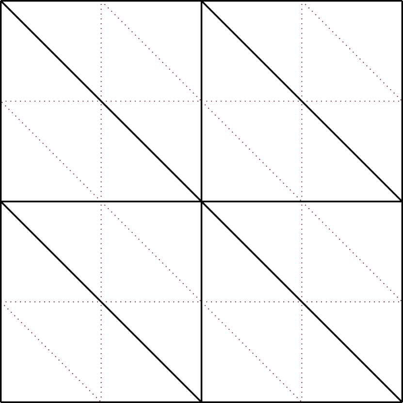
(b) $R_{\mathcal{U}}(\Omega_{h})$

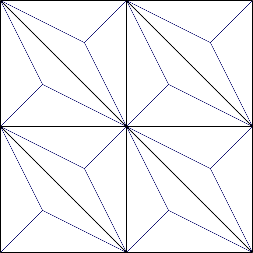
(c) $R_{\mathcal{B}}(\Omega_{h})$

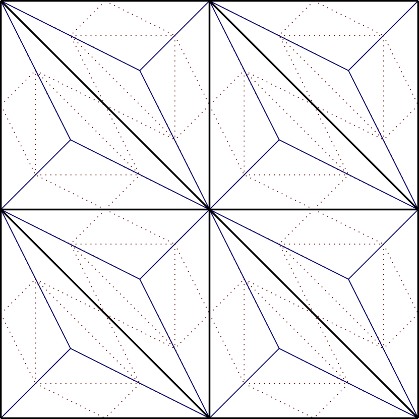
(d) $R_{\mathcal{U}}(R_{\mathcal{B}}(\Omega_{h}))$

Figure 1: Mesh refinements. (a) structured 2D triangular mesh; (b) the of (a); (c) barycentric mesh (Alfeld split), obtained via of (a); and (d) of (c).

The third discretization considered is the low-order $\boldsymbol{\mathbb{P}}_{1}\text{iso}\kern 1.0pt\boldsymbol{\mathbb{P}}_{2}/\mathbb{P}_{1}$ discretization. It is well known that a mixed discretization using piecewise linear finite elements for both velocities and pressures, such as $\boldsymbol{\mathbb{P}}_{1}/\mathbb{P}_{1}$, does not satisfy the necessary inf-sup stability criterion for well-posedness. The $\boldsymbol{\mathbb{P}}_{1}\text{iso}\kern 1.0pt\boldsymbol{\mathbb{P}}_{2}/\mathbb{P}_{1}$ gets around this instability by considering first-order discretizations of both velocities and pressures, but on different meshes. Specifically, the $\boldsymbol{\mathbb{P}}_{1}$ velocity space is discretized on a quadrisection refinement, $R_{\mathcal{U}}(\Omega_{h})$, of the mesh, $\Omega_{h}$, used for the $\mathbb{P}_{1}$ discretization of the pressure. The $\boldsymbol{\mathbb{P}}_{1}\text{iso}\kern 1.0pt\boldsymbol{\mathbb{P}}_{2}/\mathbb{P}_{1}$ discretization is known to be inf-sup stable [38] but is not commonly used due to its relatively low accuracy and computational efficiency. Here, we make use of this discretization not to directly approximate solutions to the Stokes equations but, instead, as an auxiliary operator with which we build preconditioners for the discretizations of interest above.

Figure 1 illustrates meshes used in the construction of the $\boldsymbol{\mathbb{P}}_{2}/\mathbb{P}_{1}$, $\boldsymbol{\mathbb{P}}_{2}/\mathbb{P}_{1}^{disc}$, and $\boldsymbol{\mathbb{P}}_{1}\text{iso}\kern 1.0pt\boldsymbol{\mathbb{P}}_{2}/\mathbb{P}_{1}$ systems. In all cases, we consider a given mesh, $\Omega_{h}$, as shown in Figure 1(a). We denote the quadrisection refinement of $\Omega_{h}$, by $R_{\mathcal{U}}(\Omega_{h})$, as shown in Figure 1(b). Similarly, Figure 1(c) denotes the barycentric refinement of $\Omega_{h}$, $R_{\mathcal{B}}(\Omega_{h})$. For the SV discretization on mesh $R_{\mathcal{B}}(\Omega_{h})$, we will make use of a quadrisection refinement of $R_{\mathcal{B}}(\Omega_{h})$, denoted $R_{\mathcal{U}}(R_{\mathcal{B}}(\Omega_{h}))$, shown in Figure 1(d).

3 Monolithic Multigrid

In this section, we introduce our multilevel algorithm for solving the Stokes system, $Kx=b$, referenced in Equation 3. The algorithm comprises several key components that we will detail in subsequent sections, namely:

• the use of the low-order $\boldsymbol{\mathbb{P}}_{1}\text{iso}\kern 1.0pt\boldsymbol{\mathbb{P}}_{2}/\mathbb{P}_{1}$ discretization to precondition the system;

• the construction of algebraic multigrid hierarchies for separate portions of the system, including the vector Laplacian on the velocity variables (represented by $A$) and the div-grad-like system for pressure;

• a careful algebraic coarsening of the $(\bm{u},p)$ degrees-of-freedom (DoFs) that mimics the behavior observed in efficient geometric multigrid schemes for Stokes;

• an algebraic form of Vanka relaxation for saddle-point systems, with a tuned relaxation parameter; and

• block LU factorization technique for the solution of Vanka patches that greatly reduces storage and computational cost.

In total, the algorithm derived in this section (and presented in detail in Algorithm 1) is algebraic in fashion, requiring only a description of the original (fine) DoFs and a low-order interpolation operator based on the finite-element basis (on the fine level).

3.1 Low-Order Preconditioning

In [19], we demonstrate that the low-order $\boldsymbol{\mathbb{Q}}_{1}\text{iso}\kern 1.0pt\boldsymbol{\mathbb{Q}}_{2}/\mathbb{Q}_{1}$ finite-element discretization can be leveraged to construct efficient and robust geometric multigrid (GMG) preconditioners for the higher-order $\boldsymbol{\mathbb{Q}}_{2}/\mathbb{Q}_{1}$ discretization of the Stokes equations. In that work, a multilevel defect-correction approach was proposed that we follow here. There are two aims in the present work. First, to extend the approach of [19] from two-dimensional quadrilateral meshes to triangular and tetrahedral meshes, allowing it to be applied to a wider range of scenarios, including more discretizations and unstructured grids. Secondly, we aim to construct the defect-correction preconditioner in an algebraic setting without relying on geometric information about the mesh to construct interpolation (or other) operators.

Let $K_{0}$ and $K_{1}$ be the Stokes operators assembled using a higher-order discretization (either $\boldsymbol{\mathbb{P}}_{2}/\mathbb{P}_{1}$ or $\boldsymbol{\mathbb{P}}_{2}/\mathbb{P}_{1}^{disc}$) and the lower-order $\boldsymbol{\mathbb{P}}_{1}\text{iso}\kern 1.0pt\boldsymbol{\mathbb{P}}_{2}/\mathbb{P}_{1}$ discretization, respectively, where the pressure for the $\boldsymbol{\mathbb{P}}_{1}\text{iso}\kern 1.0pt\boldsymbol{\mathbb{P}}_{2}/\mathbb{P}_{1}$ discretization is defined on the same grid as the higher-order discretization, and the $\boldsymbol{\mathbb{P}}_{1}\text{iso}\kern 1.0pt\boldsymbol{\mathbb{P}}_{2}$ velocity is defined on the quadrisection refinement of this mesh. As the spaces associated with $K_{0}$ and $K_{1}$ are different, transfer operators are needed to map from the low-order mesh to the high-order mesh, denoted by $P_{0}$, and vice-versa, denoted by $R_{0}$. Further, let $G_{1}$ denote the error-propagation operator for a stationary iterative solver for $K_{1}$. Extending [19], we consider a defect-correction algorithm defined by the two-level iteration scheme with the error-propagation operator

$$G_{dc}=\left(I-\omega_{0}M_{0}^{-1}K_{0}\right)^{\nu_{2}}\left(I-P_{0}(I-G_{1}^{\gamma})K_{1}^{-1}\eta R_{0}K_{0}\right)\left(I-\omega_{0}M_{0}^{-1}K_{0}\right)^{\nu_{1}}.$$ (4)

Here, $\nu_{1}$ relaxation sweeps are first applied to the $K_{0}$ operator where the specific relaxation scheme is defined by the choice of $M_{0}^{-1}$. This is followed by a coarse/low-order correction given by the middle expression, followed by post-relaxation on $K_{0}$. The low-order correction includes first a high-order residual calculation (the $K_{0}$ term) which is restricted using $\eta R_{0}$. Then, $\gamma$ iterations of the $G_{1}$ solver are used to produce a low-order approximate solution that is interpolated via $P_{0}$ back the fine space. We note that if $\gamma=\infty$ and $G_{1}$ is a convergent iteration, then the middle term reduces to $\left(I-P_{0}K_{1}^{-1}\eta R_{0}K_{0}\right)$, which corresponds to solving the coarse problem exactly. As we demonstrate in Section 4, an important (and non-standard) feature of this cycle is the residual weighting operator, $\eta$. Here, $\eta$ is a $2\times 2$ block-diagonal matrix that imposes separate scaling of residual equations corresponding to the momentum, Equation 1a, and the continuity, Equation 1b, equations, by scalar weights $\eta_{u}$ and $\eta_{p}$, and is represented by the following operator:

$$\eta=\begin{bmatrix}\eta_{u}I&\\ &\eta_{p}I\end{bmatrix}.$$ (5)

Depending on the construction of the $K_{0}$ discretization, we find two useful regimes for the scaling parameters, $\eta_{u}$ and $\eta_{p}$. When $K_{0}$ comes from the $\boldsymbol{\mathbb{P}}_{2}/\mathbb{P}_{1}$ discretization, we find it is productive to use $\eta_{p}\approx\eta_{u}\leq 1$, damping the defect correction from the $K_{1}$ discretization. In contrast, when $K_{0}$ comes from the $\boldsymbol{\mathbb{P}}_{2}/\mathbb{P}_{1}^{disc}$ discretization, we find $\eta_{p}\gg\eta_{u}\approx 1$, or continuity equation residual overweighting, is the most effective. We note that residual overweighting has been used to accelerate the convergence of non-Galerkin defect-correction multigrid methods by minimizing the discrepancy between levels in other contexts [39, 40]. We also note that, in the work below, we do not introduce additional residual weighting between levels in the multigrid cycle for $K_{1}$, as preliminary experiments found that this did not lead to further improvements in convergence.

We construct the grid transfer operator, $P_{0}$, between the higher-order ($K_{0}$) and the low-order ($K_{1}$) discretization as a block-diagonal matrix

$$P_{0}=\begin{bmatrix}P^{\bm{u}}_{0}&\\ &P^{p}_{0}\end{bmatrix},$$ (6)

where $P^{\bm{u}}_{0}$ and $P^{p}_{0}$ correspond to velocity and pressure field interpolation operators. For the $K_{0}$ and $K_{1}$ system discretized with $\boldsymbol{\mathbb{P}}_{2}/\mathbb{P}_{1}$ and $\boldsymbol{\mathbb{P}}_{1}\text{iso}\kern 1.0pt\boldsymbol{\mathbb{P}}_{2}/\mathbb{P}_{1}$ elements, respectively, the pressure and velocity unknowns are co-located; therefore, it is plausible to use injection operators, $P^{\bm{u}}_{0}=I$ and $P^{p}_{0}=I$, as in [19]. Formally, element projection (described at the end of this paragraph) is a natural way to define a restriction operator that maps between two different spaces. However, given the co-located nature of the degrees of freedom, it is convenient to simply use injection to define restriction for $\boldsymbol{\mathbb{P}}_{2}/\mathbb{P}_{1}$ and $\boldsymbol{\mathbb{P}}_{1}\text{iso}\kern 1.0pt\boldsymbol{\mathbb{P}}_{2}/\mathbb{P}_{1}$ discretizations, and so $R_{0}=P_{0}^{T}$. For the $\boldsymbol{\mathbb{P}}_{2}/\mathbb{P}_{1}^{disc}$ operator, $K_{0}$, it is still convenient to use injection for the velocity degrees of freedom, as the $\boldsymbol{\mathbb{P}}_{1}\text{iso}\kern 1.0pt\boldsymbol{\mathbb{P}}_{2}$ velocity degrees of freedom in $K_{1}$ are again co-located with those of $K_{0}$, again leading to $P^{\bm{u}}_{0}=R^{\bm{u}}_{0}=I$. For the pressure degrees of freedom, however, more complicated mappings are needed, as $K_{0}$ uses discontinuous piecewise-linear basis functions, while $K_{1}$ uses continuous piecewise-linear basis functions on the same mesh. Thus, there are approximately six times as many DoFs in the $\mathbb{P}_{1}^{disc}$ pressure field as in the $\mathbb{P}_{1}$ pressure in 2D (since there are approximately twice as many elements on a (regular) triangular mesh as nodes, and three pressure DoFs per element for the $\mathbb{P}_{1}^{disc}$ discretization compared to one per node for $\mathbb{P}_{1}$). Since $\mathbb{P}_{1}{}\subset\mathbb{P}_{1}^{disc}{}$, interpolation, $P^{p}_{0}$, is naturally given by finite-element interpolation, determining the coefficients in the $\mathbb{P}_{1}^{disc}$ basis that correspond to a given function in $\mathbb{P}_{1}$. In the case when the discontinuous pressure degrees of freedom are co-located at the mesh nodes (with one DoF for each adjacent element), this mapping is simply the duplication of the continuous pressure value at the node to each discontinuous DoF associated with the node, and its discrete structure is easy to infer from the mesh and associated operators. Since $\mathbb{P}_{1}^{disc}{}\not\subset\mathbb{P}_{1}{}$, however, direct injection or averaging of the discontinuous DoFs when restricting from $\mathbb{P}_{1}^{disc}$ to $\mathbb{P}_{1}$ space is not as straightforward. Instead, we define the restriction operator, $R^{p}_{0}$, applied to a function, $p_{dg}\in\mathbb{P}_{1}^{disc}{}$ yielding its corresponding continuous analog, $p_{cg}$, by finite-element projection. That is, we compute $p_{cg}\in\mathbb{P}_{1}{}$ that satisfies $\langle p_{cg},q_{cg}\rangle=\langle p_{dg},q_{cg}\rangle$ for all $q_{cg}$ in the $\mathbb{P}_{1}$ space. As both $p_{cg}$ and $q_{cg}$ can be expressed in terms of basis functions, this leads to solving a matrix equation involving a standard $\mathbb{P}_{1}$ mass matrix, where the right-hand side is also naturally defined in terms of the basis functions of the two spaces. In either case, we assemble both $P_{0}$ and $R_{0}$ at the same time as we assemble the $K_{0}$ and $K_{1}$ discretization matrices, and (if needed) approximate the inverse of the $\mathbb{P}_{1}$ mass matrix by FGMRES preconditioned with a standard scalar AMG solver to an $\ell_{2}$ norm of the relative residual of $10^{-12}$. The number of iterations needed to achieve this does not increase with the refinement level.

Remark 1 ($\boldsymbol{\mathbb{P}}_{2}/\mathbb{P}_{1}$ to $\boldsymbol{\mathbb{P}}_{1}\text{iso}\kern 1.0pt\boldsymbol{\mathbb{P}}_{2}/\mathbb{P}_{1}$ Grid-Transfer Operators)

A natural question is whether the analogous finite-element projection operators should be used to transfer residuals and corrections between the non-nested velocity spaces $\boldsymbol{\mathbb{P}}_{2}$ and $\boldsymbol{\mathbb{P}}_{1}\text{iso}\kern 1.0pt\boldsymbol{\mathbb{P}}_{2}$ for both higher-order Stokes discretizations. To examine this in a simpler setting, we considered using AMG applied to the $\mathbb{Q}_{1}\text{iso}\kern 1.0pt\mathbb{Q}_{2}$ discretization as a preconditioner for the $\mathbb{Q}_{2}$ discretization of a scalar Poisson problem on the unit square. In this setting, using finite-element projection to define $R_{0}$ did not significantly improve performance, leading to a maximum improvement of only one or two iterations in any given solve. Given this limited improvement in performance and increased cost and complexity of assembling the projection operators, we do not make use of this approach for the grid transfers between $\boldsymbol{\mathbb{P}}_{2}$ and $\boldsymbol{\mathbb{P}}_{1}\text{iso}\kern 1.0pt\boldsymbol{\mathbb{P}}_{2}$ here, but note that using proper projections may show more benefit in other settings.

3.2 Smoothed Aggregation AMG for the Stokes Operator

The standard two-level error-propagation operator for a multigrid cycle is given by

$$G_{\ell}=(I-\omega_{\ell}M_{\ell}^{-1}K_{\ell})^{\nu_{2}}(I-P_{\ell}K_{\ell+1}^{-1}R_{\ell}K_{\ell})(I-\omega_{\ell}M_{\ell}^{-1}K_{\ell})^{\nu_{1}}\text{ for }\ell>0,$$ (7)

where $\ell$ denotes the level within the multigrid hierarchy, $K_{\ell}$ is the level-$\ell$ system matrix, $M_{\ell}$ represents the relaxation operator applied to $K_{\ell}$ with damping parameter $\omega_{\ell}$, $P_{\ell}$ is the interpolation between levels $\ell+1$ and $\ell$, and $R_{\ell}$ is the restriction from level $\ell$ to level $\ell+1$. $G_{1}$, for example, defines a two-level solver within (4) to approximately solve the $K_{1}$ system. For algebraic multigrid methods, $K_{\ell+1}$ is almost always taken as $K_{\ell+1}=P_{\ell}^{T}K_{\ell}P_{\ell}$, and a standard multigrid algorithm replaces the $K_{\ell+1}$ solve with a recursive application of the two-grid solver. The multilevel cycle is fully specified once the $P_{\ell},R_{\ell}$, $K_{\ell+1}$, and $M_{\ell}$ are defined for all hierarchy levels. In this paper, we take $R_{\ell}=P_{\ell}^{T}$ and $K_{\ell+1}=P_{\ell}^{T}K_{\ell}P_{\ell}$ within the AMG hierarchy (for $\ell\geq 1$) and, so, only algorithms for $P_{\ell}$ and $M_{\ell}$ needed to be determined.

The central feature of AMG is the automatic definition of interpolation operators, $P_{\ell}$, based only on $K_{\ell}$, with minimal further information. While popular AMG algorithms can be directly applied to our $\boldsymbol{\mathbb{P}}_{1}\text{iso}\kern 1.0pt\boldsymbol{\mathbb{P}}_{2}/\mathbb{P}_{1}$ system, we find that these generally do not lead to fast convergence in the resulting solvers. Of course, most popular AMG algorithms were originally designed for scalar PDEs coming from elliptic equations that often give rise to positive-definite matrices, or even M-matrices. While many of these AMG techniques are also effective for elliptic PDE systems, such as the vector- Laplacian, they are generally not directly applicable to saddle point systems. For example, standard smoothed aggregation (SA) AMG (as implemented, for example, in PyAMG [41]) essentially assumes that a damped Jacobi relaxation scheme converges and smooths errors when applied to the system matrix, neither of which is true for saddle-point systems such as $K_{1}$, for which it is not even well-defined, due to the zero diagonal block in the matrix.

To apply AMG to our system, we consider defining block-structured grid transfer operators, as were used in (6) to determine $P_{0}$, and then apply AMG algorithms to define the individual blocks of the interpolation matrix. This structure ensures that fine-level pressures (velocities) interpolate only from coarse-level pressures (velocities), and not from coarse-level velocities (pressures). For the velocity block, since the vector Laplacian is an elliptic PDE and we discretize it using vector $\boldsymbol{\mathbb{P}}_{1}$ elements, most AMG algorithms can be reliably applied to $A$ to produce a suitable $P^{\bm{u}}_{0}$ for the velocity interpolation operator. AMG cannot, however, be directly applied to the zero diagonal block associated with pressure, so some auxiliary operator is needed to determine the pressure interpolation. One possible choice for this auxiliary matrix is the associated pressure Laplacian, $A_{p}$, discretized using the $\mathbb{P}_{1}$ pressure basis functions. Certainly, many common AMG algorithms are effective when applied to standard discrete Laplace operators, producing convergent cycles with effective choices for the grid-transfer operators. Using $A_{p}$ has the disadvantage that it requires an additional matrix for the AMG setup process, albeit one that is easily generated using any finite-element package. An alternative and purely algebraic auxiliary operator is $BB^{T}$, perhaps in conjunction with some type of truncation of the stencil [14]. $BB^{T}$ also represents a discrete form of the Laplace operator, although it generally has a somewhat wider stencil than $A_{p}$, which can prove challenging for AMG coarsening algorithms. In the remainder of the paper, we use $A_{p}$, assembled with the canonical pressure basis on the fine grid, to avoid the introduction of additional tuning parameters associated with truncating $BB^{T}$.

Algorithm 1 details our setup of the multigrid hierarchy for the 2D case, assuming either direct access to each block of the Stokes systems in Equation 3, or being able to infer $A$ and $B$ from $K_{1}$, based on the knowledge of the total number of discrete degrees of freedom in each field. While a systems version of SA-AMG could be applied directly to the vector Laplacian, we instead apply a scalar version of SA-AMG to each component of the vector Laplacian. As expected, the two approaches yield similar aggregates and interpolation operators, assuming the systems SA-AMG algorithm is provided the two-dimensional near-kernel space,

$${\cal N}_{v}=\begin{bmatrix}\bm{1}_{n_{x}}&\\ &\bm{1}_{n_{y}}\\ \end{bmatrix}.$$ (8)

where $\bm{1}_{k}$ refers to a length $k$ vector with all entries equal to one. We note that the systems approach may be advantageous when considering problems with complex boundary conditions, or generalized operators where $A$ is not a block-diagonal matrix. Since we independently coarsen the velocity and pressure blocks, SA-AMG may determine different numbers of levels in each hierarchy. Thus, we form a block hierarchy using the fewest levels across these hierarchies. While this could lead to impractically large coarsest-grid systems if the coarsening of each field is dramatically different, we have yet to see any such problems in work to date. After the interpolation operators for each field are formed, they are combined as a block-diagonal matrix into a single monolithic interpolation operator $P_{\ell}$, and used in a monolithic calculation of the coarse-grid operator.

1:Input: $K_{1}=\begin{bmatrix}A&B^{T}\\ B&\end{bmatrix}$, Stokes system where $B\in\mathbb{R}^{n_{p}\times(n_{x}+n_{y})}$

2:           $A_{p}$, pressure stiffness matrix or a truncated version of $BB^{T}$

3:Output: $K_{1},$…$,K_{\ell_{max}}$, Grid hierarchy

4:              $P_{1},$…$,P_{\ell_{max}-1}$, Interpolation Operators

5:

6:$A_{x}$, $A_{y}$ = split(A) // Split vector Laplacian component-wise

7:$\{P_{1}^{x},\dots,P_{\ell}^{x},\dots P_{\ell^{x}_{\text{max}}-1}^{x}\}=\text{sa\_amg}(A_{x},\bm{1}_{n_{x}})$ // Construct interpolation for velocity in $x$

8:$\{P_{1}^{y},\dots,P_{\ell}^{y},\dots P_{\ell^{y}_{\text{max}}-1}^{y}\}=\text{sa\_amg}(A_{y},\bm{1}_{n_{y}})$ // Construct interpolation for velocity in $y$

9:$\{P_{1}^{p},\dots,P_{\ell}^{p},\dots P_{\ell^{p}_{\text{max}}-1}^{p}\}=\text{sa\_amg}(A_{p},\bm{1}_{n_{z}})$// Construct interpolation for pressure

10:$\ell_{max}=\text{min}\left(\ell^{x}_{\text{max}},\ell^{y}_{\text{max}},\ell^{p}_{\text{max}}\right)$ // Calculate levels in grid hierarchy

11:

12:for $\ell=1,\ldots,\ell_{max}-1$ do

13:     $P_{\ell}=\begin{bmatrix}P^{x}_{\ell}&&\\ &P^{y}_{\ell}&\\ &&P^{p}_{\ell}\end{bmatrix}$ // Assemble monolithic interpolation operator

14:     $K_{\ell+1}=P_{\ell}^{T}K_{\ell}P_{\ell}$ // Compute coarse-grid operator

15:end for

Algorithm 1 SA-AMG Hierarchy Setup for 2D Stokes System

We emphasize that we use smoothed aggregation completely independently on each field (7, 8, and 9 in Algorithm 1), without any explicit coordination or coupling (in contrast to most traditional monolithic MG methods). As a result, the $B$ block in $K$ is projected to its coarse-grid analog using both the velocity and pressure grid transfers. A natural concern is whether this independent coarsening might lead to somewhat strange stencils in $B$, where the coarse-grid discretization might not necessarily even be stable, even if the fine-level $B$ is stable. While our approach does not guarantee stability, we have observed that we generally get stable coarse-grid operators so long as we maintain a similar ratio between the velocity and pressure DoFs throughout the hierarchy, which is crucial to the convergence of the overall AMG method. This can be achieved when we (approximately) match the coarsening rates for each field on each level. These coarsening rates are effectively determined by the strength-of-connection (SoC) measures used in aggregation, which identify the edges of the matrix graph that can be ignored during the coarsening process. Using traditional SoC measures, such as the symmetric strength of connection commonly used in smoothed aggregation [42], we found that achieving compatible coarsening rates was difficult, requiring significant tuning of drop-tolerance parameters for the velocity and pressure fields at each level of the hierarchy. Instead, we employ the so-called evolution SoC from [43], which provides more uniform coarsening by integrating local representations of algebraically smooth error into the SoC measures. We observe (experimentally) that this leads to consistent coarsening rates across the velocity and pressure fields, with no need for parameter tuning [44].

Remark 2 (Applying Algorithm 1 directly to $K_{0}$)

Algorithm 1 can also be applied directly to the $\boldsymbol{\mathbb{P}}_{2}/\mathbb{P}_{1}$ discretization of the matrix $K_{0}$, resulting in a preconditioner that we denote by HO-AMG. While the effectiveness of HO-AMG is expected to decline for discretizations with higher-order bases due to mismatch in pressure and velocity field coarsening rates, we find that it offers stable performance for the $\boldsymbol{\mathbb{P}}_{2}/\mathbb{P}_{1}$ discretization considered here.

The direct application of Algorithm 1 to the $\boldsymbol{\mathbb{P}}_{2}/\mathbb{P}_{1}^{disc}$ discretization of the $K_{0}$ system, on the other hand, leads to either poorly convergent or non-convergent preconditioners, which we attribute to limitations in the algebraic coarsening of the discontinuous pressure field.

3.3 Relaxation

The final piece of the monolithic AMG method for Stokes is the coupled relaxation method with (weighted) error propagation operator $I-\omega_{\ell}M_{\ell}^{-1}K_{\ell}$. Vanka relaxation [6] is a standard relaxation scheme for saddle-point problems, using an overlapping domain-decomposition approach to improving an approximation to the solution of the global system via local “patch” solves over small sets of DoFs within a standard additive or multiplicative Schwarz method.

A Vanka patch is typically constructed to contain a small number of pressure DoFs (often just one) and all velocity DoFs that are adjacent (i.e., have nonzero connections) to this “seed” pressure DoF in the system matrix, $K$. Within geometric multigrid, such patches can be naturally constructed using topological arguments [45]; here, however, we construct the patches algebraically on each level of the hierarchy. Although the general mechanism for patch assembly is the same for all discretizations, we define each patch with a single seed pressure DoF for both the $\boldsymbol{\mathbb{P}}_{1}\text{iso}\kern 1.0pt\boldsymbol{\mathbb{P}}_{2}/\mathbb{P}_{1}$ multigrid hierarchy and the fine-grid $\boldsymbol{\mathbb{P}}_{2}/\mathbb{P}_{1}$ discretization. In these cases, each row of $B$ corresponds to one patch, and each patch $i$ incorporates the DoF $i$ of the pressure and all velocity DoFs linked to nonzero entries in row $i$ of $B$. The patch construction process differs according to the specific discretization.

With the $\boldsymbol{\mathbb{P}}_{2}/\mathbb{P}_{1}^{disc}$ discretization, we employ three seed pressure DoFs for each patch, corresponding to the three pressure DoFs within each element. The three pressure DoFs on each element can be identified by three rows of $B$ with identical sparsity patterns, making it possible to determine the seeds algebraically. However, since the information is readily available and requires minimal pre-processing, we opt to use a straightforward element-to-DoF map to identify the three pressure DoFs on a single element. Figure 2 depicts typical patches for the $\boldsymbol{\mathbb{P}}_{2}/\mathbb{P}_{1}^{disc}$, $\boldsymbol{\mathbb{P}}_{2}/\mathbb{P}_{1}$ and $\boldsymbol{\mathbb{P}}_{1}\text{iso}\kern 1.0pt\boldsymbol{\mathbb{P}}_{2}/\mathbb{P}_{1}$ discretizations of the fine-level operators. We note that these patches have a direct (topological) connection to the element/mesh entities on the finest mesh; however, there is no simple element/mesh interpretation on algebraically coarsened levels.

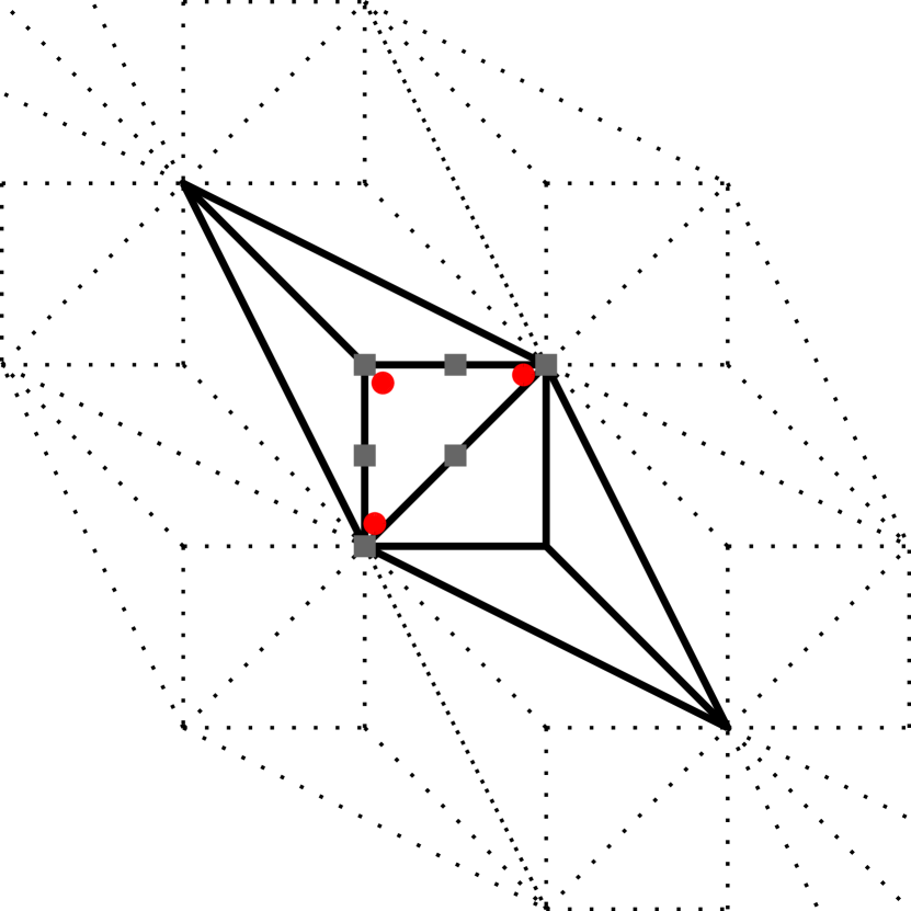
(a) $\boldsymbol{\mathbb{P}}_{2}/\mathbb{P}_{1}^{disc}$

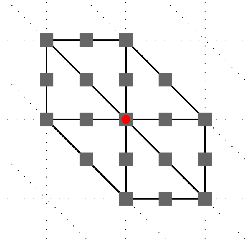
(b) $\boldsymbol{\mathbb{P}}_{2}/\mathbb{P}_{1}$

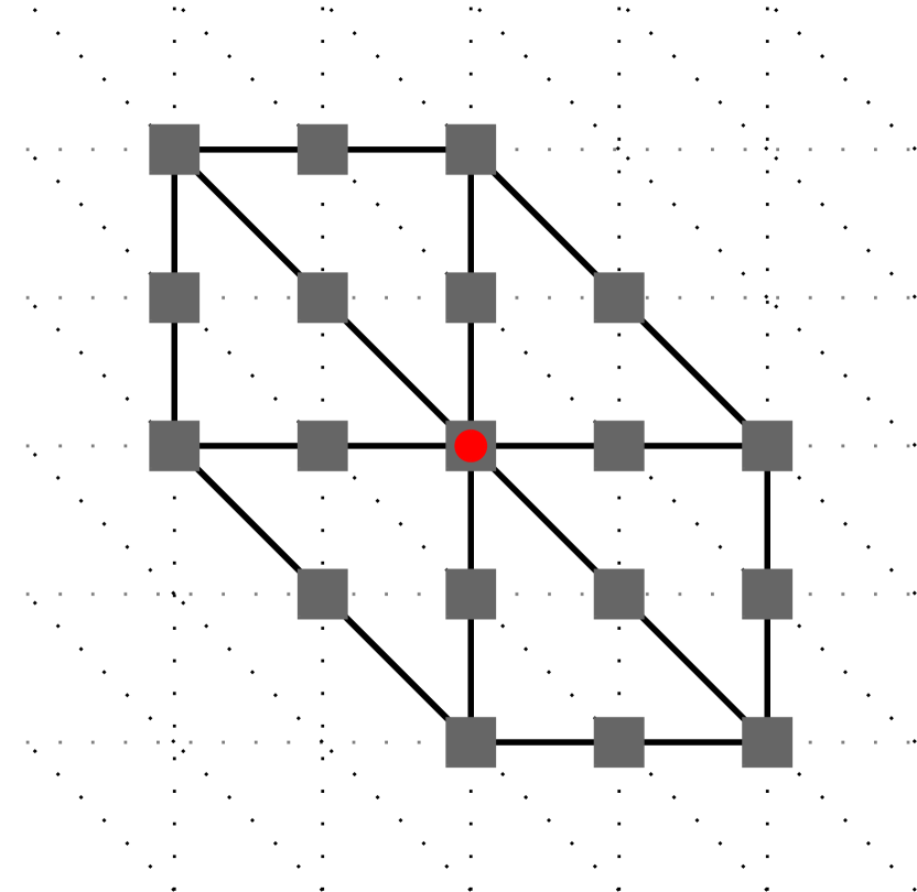
(c) $\boldsymbol{\mathbb{P}}_{1}\text{iso}\kern 1.0pt\boldsymbol{\mathbb{P}}_{2}/\mathbb{P}_{1}$

Figure 2: (Left) one Vanka patch for the $\boldsymbol{\mathbb{P}}_{2}/\mathbb{P}_{1}^{disc}$ discretization; (middle) one Vanka patch for the $\boldsymbol{\mathbb{P}}_{2}/\mathbb{P}_{1}$ discretization; and (right) one Vanka patch for the $\boldsymbol{\mathbb{P}}_{1}\text{iso}\kern 1.0pt\boldsymbol{\mathbb{P}}_{2}/\mathbb{P}_{1}$ discretization. The pressure DoF(s) (red circles, ) and the velocity DoFs directly algebraically connected to that pressure DoF (gray squares, ) are marked. Displayed patched are on 2D triangular meshes.

On level $\ell$, the $i^{th}$ patch matrix $K_{\ell}^{(i)}$ is then given by a square sub-matrix, which is composed of patch sub-blocks $B^{(i)}$ and $A^{(i)}$, written as

$$K_{\ell}^{(i)}=\begin{bmatrix}A^{(i)}&(B^{(i)})^{T}\\ B^{(i)}&0\end{bmatrix}.$$ (9)

Formally, $K_{\ell}^{(i)}=V_{\ell}^{(i)}K_{\ell}(V_{\ell}^{(i)})^{T}$ where $V_{\ell}^{(i)}$ is an injection operator defined for each patch, $i$, on level $\ell$ as an $m^{(i)}_{\ell}\times m_{\ell}$ binary matrix that extracts the subset of global DoFs on level $\ell$ coinciding with the $i^{\text{th}}$ patch, where $m_{\ell}$ is the total number of rows / columns of $K_{\ell}$, while $m^{(i)}_{\ell}$ is the number of DoFs contained in $K_{\ell}^{(i)}$, which is one more than the number of velocity DoFs in the $i^{th}$ patch for the $\boldsymbol{\mathbb{P}}_{1}\text{iso}\kern 1.0pt\boldsymbol{\mathbb{P}}_{2}/\mathbb{P}_{1}$ and $\boldsymbol{\mathbb{P}}_{2}/\mathbb{P}_{1}$ discretizations, and three more for the $\boldsymbol{\mathbb{P}}_{2}/\mathbb{P}_{1}^{disc}$ discretization.

In this work, we use the additive form of Vanka relaxation [9, 46]. A single sweep of Vanka relaxation for $\boldsymbol{\mathbb{P}}_{1}\text{iso}\kern 1.0pt\boldsymbol{\mathbb{P}}_{2}/\mathbb{P}_{1}$ and $\boldsymbol{\mathbb{P}}_{2}/\mathbb{P}_{1}$ discretizations is then given by

$$M^{-1}_{\ell}=\sum_{i=1}^{n^{(p)}_{\ell}}(V_{\ell}^{(i)})^{T}W_{\ell}^{(i)}\left(V_{\ell}^{(i)}K_{\ell}(V_{\ell}^{(i)})^{T}\right)^{-1}V_{\ell}^{(i)},$$

where the diagonal weighting matrix, $W_{\ell}^{(i)}$, is a partition of unity, with each diagonal entry equal to the reciprocal of the number of patches that contain the associated degree of freedom. For the $\boldsymbol{\mathbb{P}}_{2}/\mathbb{P}_{1}^{disc}$ discretization, the sum extends over fewer patches, for $1\leq i\leq n^{(p)}_{\ell}/3$.

Applying the inverses of patch matrices often constitutes the most computationally demanding part of the multigrid method. Several strategies are available for applying the inverse of the patch $K_{\ell}^{(i)}$, each with distinct advantages and disadvantages. The direct inverse of the patch can be applied using highly optimized dense-linear algebra kernels. However, this approach requires significant storage, as it results in a fully dense operator over each patch. Alternatively, sparse LU factorization of patches could be employed to achieve the patch inverse action. This approach has much lower memory cost, but results in slower solution times, due to the associated sparse forward and backward substitutions. Our performance studies, not shown here, indicated the sparse LU technique did not surpass the direct-inverse method in efficiency. Nonetheless, the substantial storage requirements linked with dense inverses may be restrictive.

Therefore, we introduce a novel approach that tries to balance the effectiveness of dense-linear algebra routines with the reduced storage demands of sparse LU factorizations. Instead of directly computing the inverse of each $K_{\ell}^{(i)}$, we instead leverage a block LU factorization of each Vanka patch. Equation 10 illustrates this procedure for a Vanka patch, with sub- and superscripts on the sub-blocks being omitted for clarity, writing

$$K_{\ell}^{(i)}=\begin{bmatrix}A&B^{T}\\ B&0\end{bmatrix}=\begin{bmatrix}A&\\ B&S\end{bmatrix}\begin{bmatrix}I&U\\ &I\end{bmatrix},$$ (10)

where $U=A^{-1}B$, and $S=-BA^{-1}B^{T}$ denotes the Schur complement. We emphasize here that $B^{T}$ and $U$ have small column dimension (one in the typical case, but three for the $\boldsymbol{\mathbb{P}}_{2}/\mathbb{P}_{1}^{disc}$ discretization), and that $S$ is a small matrix. Equation 11 expresses the action of the inverse for the block-factorized Vanka patch matrices, with $\hat{B}=-S^{-1}BA^{-1}$, $\hat{U}=-U$, and operators $\hat{B}$, $\hat{U}$, and $S^{-1}$ recommended to be precomputed in the setup phase,

$$K_{\ell}^{(i)}x_{\ell}^{(i)}=b_{\ell}^{(i)}\;\Rightarrow\;x_{\ell}^{(i)}=\begin{bmatrix}I&\hat{U}\\ &I\end{bmatrix}\begin{bmatrix}A^{-1}&\\ \hat{B}&S^{-1}\end{bmatrix}b_{\ell}^{(i)}.$$ (11)

We further leverage the block-diagonal nature of the vector-Laplacian operator to minimize the storage costs associated with the inverse of sub-block $A$ up to a factor of 2 and 3 in 2D and 3D, respectively. Furthermore, this method reduces the number of floating-point operations necessary for calculating the action of the patch’s inverse, thereby enhancing the computational efficiency of the setup and solution phases.

As with many multigrid relaxation schemes, Vanka relaxation is known to be sensitive to the choice of the damping parameter, $\omega_{\ell}$. Fourier analysis is often used to determine $\omega_{\ell}$ when Vanka is employed within a GMG scheme [47, 46, 48, 49]; however, this method is not feasible for the irregular coarse meshes generated in an AMG algorithm as considered here. Several recent papers have used alternative methods to tune relaxation parameters. In [27], for example, instead of a stationary weighted relaxation scheme, a Chebyshev iteration is used, with hand-tuned Chebyshev intervals chosen to optimize the resulting solver performance. While this approach is, in principle, also applicable here, it would require significant tuning for the various levels of the multigrid hierarchy. Instead, we opt for a more practical approach where relaxation on each level is accelerated using FGMRES. FGMRES does not necessarily provide optimal relaxation weights as it constructs a residual-minimizing polynomial, which is not the same as optimally damping high-frequency error. While it does not provide general convergence bounds as can sometimes be achieved using Chebyshev iterations, it does eliminate the need for additional tuning parameters and generally provides satisfactory damping weights. One minor drawback is that FGMRES requires additional inner products, though this is a minimal computational cost over the Vanka relaxation patch solves.

In the remainder of the paper, we fix the relaxation to include two inner FGMRES iterations with one Vanka relaxation sweep per iteration, akin to setting $\nu_{1}=\nu_{2}=2$ in (4) or (7). Results below show that using this Krylov wrapping approach on all levels in the hierarchy provides stable and robust convergence for systems discretized with $\boldsymbol{\mathbb{P}}_{2}/\mathbb{P}_{1}$ elements. However, we observed stagnant convergence when applied to systems discretized with $\boldsymbol{\mathbb{P}}_{2}/\mathbb{P}_{1}^{disc}$ elements. To address this issue, we instead use a stationary Vanka iteration on the finest grid with the $\boldsymbol{\mathbb{P}}_{2}/\mathbb{P}_{1}^{disc}$ elements (in (4)) and Krylov acceleration on all other levels (in (7)). We perform a parameter search to identify the optimal $\omega_{0}$ value, denoted as $\omega_{0}^{opt}$, for the $K_{0}$ systems discretized with the $\boldsymbol{\mathbb{P}}_{2}/\mathbb{P}_{1}^{disc}$ element pair, discussed below.

4 Numerical Results

In this section, we evaluate the performance of two types of monolithic AMG preconditioners, namely HO-AMG and the defect-correction method. The HO-AMG preconditioner is constructed by applying Algorithm 1 directly to the high-order discretization ($K_{0}$), while defect correction applies Algorithm 1 to an auxiliary operator, $K_{1}$. For the defect-correction (DC) preconditioners, we consider three different relaxation schedules: DC-all, DC-skip1, and DC-skip0. The DC-all preconditioner performs pre- and post-relaxation on all levels of the hierarchy, except for the coarsest level ($n_{lvls}$) where an exact solution is used. DC-skip1 skips relaxation on the $K_{1}$ system, but performs relaxation on the $K_{0}$ system and remaining levels of the $\boldsymbol{\mathbb{P}}_{1}\text{iso}\kern 1.0pt\boldsymbol{\mathbb{P}}_{2}/\mathbb{P}_{1}$ hierarchy, except for a direct solve on the coarsest level. DC-skip0 skips relaxation on the $K_{0}$ system and performs pre- and post-relaxation on remaining levels, except for a direct solve on the coarsest level. A solver diagram for the defect-correction approach is given in Figure 3. In the case of HO-AMG, the diagram reduces to Krylov solver being connected directly to Monolithic AMG based on $K_{0}$.

Figure 3: Solver diagram for defect-correction preconditioners. If relaxation is performed on all levels, the diagram corresponds to the DC-all solver.

We also explore additional preconditioning variants based on the defect-correction operator in the following sections. The notation for all relevant parameters and solvers is summarized in Table 1.

As a point of comparison for the monolithic AMG preconditioners, we employ an inexact Uzawa preconditioner [1]. The Uzawa preconditioner computes the velocity and pressure updates, $[\bm{\delta u},\delta p]$, as follows:

$$\bm{\delta u} =Q_{A}^{-1}\bm{r_{u}}$$

$$\delta p =Q_{B}^{-1}(B\bm{\delta u}-r_{p}),$$

where $[\bm{r_{u}},r_{p}]=b-Kx$, $Q_{A}^{-1}$ represents an approximation of the vector Laplacian inverse, and $Q_{B}^{-1}$ denotes an exact or approximate inverse of the pressure-mass matrix, depending on the context. To approximate $Q_{A}^{-1}$, we employ a single V-cycle of SA-AMG. For $Q_{B}^{-1}$, we use either an exact or approximate mass-matrix inverse, as outlined in [1]. The approach to $Q_{B}^{-1}$ is influenced by the discretization used. In the $\boldsymbol{\mathbb{P}}_{2}/\mathbb{P}_{1}^{disc}$ case, $Q_{B}$ is block-diagonal, enabling us to compute the exact inverse at low cost. However, when using the $\boldsymbol{\mathbb{P}}_{2}/\mathbb{P}_{1}$ discretization, we approximate the action of $Q_{B}^{-1}$ using a single V-cycle of SA-AMG. The SA-AMG solvers are assembled using evolution SoC, standard aggregation, and standard prolongator smoothing for interpolation. For multigrid relaxation, we employ two steps of Krylov-wrapped Jacobi relaxation.

Symbol	Description
$K_{0}$	saddle point system for the higher-order discretizations ($\boldsymbol{\mathbb{P}}_{2}/\mathbb{P}_{1}$, $\boldsymbol{\mathbb{P}}_{2}/\mathbb{P}_{1}^{disc}$)
$K_{1}$	saddle point system for the lower-order discretization ($\boldsymbol{\mathbb{P}}_{1}\text{iso}\kern 1.0pt\boldsymbol{\mathbb{P}}_{2}/\mathbb{P}_{1}$)
$G_{1}$	monolithic AMG Solver based on $K_{1}$
$\ell$	generic level in the monolithic multigrid hierarchy
$n_{lvls}$	total number of levels/grids in the monolithic multigrid hierarchy
$\eta_{u}$	momentum equation residual scaling parameter on level $0$
$\eta_{p}$	continuity equation residual scaling parameter on level $0$
$\eta$	$K_{0}$ residual scaling parameters when $\eta_{u}=\eta_{p}$
$\omega_{\ell}$	Vanka relaxation damping parameter
Superscript $opt$	denotes that the optimal parameter was computed via brute-force search
Uzawa	Inexact Uzawa preconditioner based on $K_{0}$
HO-AMG	Monolithic AMG algorithm applied directly on $K_{0}$
DC-all	DC with relaxation on all levels, $\omega_{\ell}=1~{}\text{for}~{}\ell\in[0,n_{lvls})$
DC-skip0	DC with relaxation on all but the $K_{0}$ level, $\omega_{\ell}=1~{}\text{for}~{}\ell\in[1,n_{lvls})$
DC-skip1	DC with relaxation on all but the $K_{1}$ level, $\omega_{\ell}=1~{}\text{for}~{}\ell\in[0]\cup[2,n_{lvls})$

Table 1: Notation Reference Table

The $\boldsymbol{\mathbb{P}}_{2}/\mathbb{P}_{1}$, $\boldsymbol{\mathbb{P}}_{2}/\mathbb{P}_{1}^{disc}$, and $\boldsymbol{\mathbb{P}}_{1}\text{iso}\kern 1.0pt\boldsymbol{\mathbb{P}}_{2}/\mathbb{P}_{1}$ systems are assembled in Firedrake [50, 51]. Although Firedrake currently does not provide the capability to construct $\boldsymbol{\mathbb{P}}_{1}\text{iso}\kern 1.0pt\boldsymbol{\mathbb{P}}_{2}/\mathbb{P}_{1}$ matrices directly, we form them by assembling the $\boldsymbol{\mathbb{P}}_{1}/\mathbb{P}_{1}$ discretization on a refined mesh and then applying geometric restriction to coarsen the pressure field. This indirect approach to forming the $\boldsymbol{\mathbb{P}}_{1}\text{iso}\kern 1.0pt\boldsymbol{\mathbb{P}}_{2}/\mathbb{P}_{1}$ discretization can be avoided in a finite-element code base that supports macro-elements. In our open-source implementation (https://github.com/Alexey-Voronin/Monolithic_AMG_For_Stokes), we use the PyAMG library [41] to implement AMG preconditioners that combine Algorithm 1 with Vanka relaxation methods.

We consider both structured and unstructured meshes in 2D and 3D for our numerical solvers study. The structured meshes are generated using the Firedrake software, while the unstructured meshes are generated using Gmsh [52]. Barycentric refinement of meshes uses the code associated with [4]. As test problems, we consider the following, with domains pictured in Figure 4.

Structured 2D: Backward-Facing Step

Here, we consider the standard 2D backward-facing step domain, discretized with structured triangular elements [1]. The left edge of the domain is marked in red in Figure 4, where a parabolic inflow boundary condition is imposed. The right edge of the domain, marked in blue, has a natural (Neumann) boundary condition. All other domain edges (marked in grey) have zero Dirichlet boundary conditions on the velocity field.

Structured 3D: Lid-Driven Cavity

Here, we consider the standard lid-driven cavity problem on a 3D domain, discretized with structured tetrahedral elements [1]. The top face of the domain, marked in red, has a Dirichlet boundary condition imposed with constant tangential velocity, while all other faces have zero Dirichlet boundary conditions on the velocity field.

Unstructured 2D: Flow Past a Cylinder

This test problem simulates flow past a cylinder on a 2D domain, discretized with unstructured triangular elements. The left edge of the domain, marked in red, has a parabolic inflow boundary condition imposed, while the right edge, marked in blue, has a natural outflow boundary condition. All other edges, including those on the interior boundary of the cylinder, have zero Dirichlet boundary conditions on the velocity field.

Unstructured 3D: Pinched Channel

This test problem simulates flow through a pinched tube on a 3D domain, discretized with unstructured tetrahedral elements. The left face of the domain, marked in red, has a constant velocity inflow boundary condition, while the right face, marked in blue, has a natural outflow boundary condition. All other faces of the domain have zero Dirichlet boundary conditions on the velocity field.

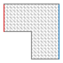
(a) 2D Structured

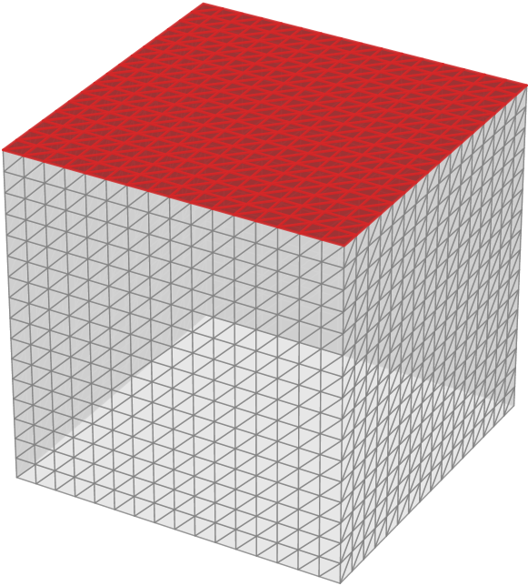
(b) 3D Structured

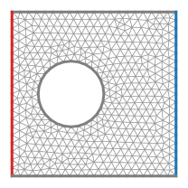
(c) 2D Unstructured

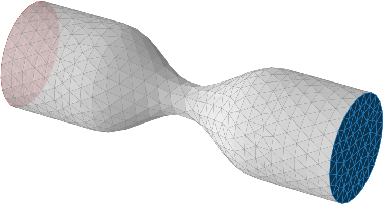
(d) 3D Unstructured

Figure 4: Meshes used to construct the Stokes problems. The boundaries are marked with three colors (red, blue, and gray), corresponding to three types of velocity field boundary conditions. Red corresponds to non-zero Dirichlet boundaries. Blue corresponds to Neumann boundary conditions. Gray indicates zero Dirichlet boundary conditions.

For each problem type, we report the iteration counts, relative time to solution, and relative time per iteration. The iteration counts are the total number of preconditioned FGMRES iterations required to reduce the $\ell_{2}$ norm of the residual by a relative factor of $10^{10}$. For all tests, we use restarted FGMRES with a maximum Krylov subspace size of $20$. The timings are measured relative to the Uzawa preconditioner. We report the shortest of five independent time-to-solution measurements to account for time measurement variability.

To find the best damping parameters, $\eta$ and $\omega_{0}$, we use a brute-force search for each problem type and multigrid variant. For the $\boldsymbol{\mathbb{P}}_{2}/\mathbb{P}_{1}$ discretization, we only have to find $\eta$, because we use Krylov-wrapping to avoid choosing $\omega_{\ell}$ on each level of the multigrid hierarchy. However, for the $\boldsymbol{\mathbb{P}}_{2}/\mathbb{P}_{1}^{disc}$ discretization, Krylov-wrapping on $\ell=0$ is not effective for achieving convergence. Therefore, for the $\boldsymbol{\mathbb{P}}_{2}/\mathbb{P}_{1}^{disc}$ DC-all preconditioner, we must calculate both $\eta$ and $\omega_{0}$. We define the optimal parameter set as the value(s) that result in the fewest number of preconditioned FGMRES iterations required to reach a relative reduction in the $l^{2}$-norm of the residual by a factor of $10^{8}$. All parameter searches were performed on problems with at least one million DoFs and 4 (3) levels in the $G_{1}$ multigrid hierarchy in 2D (3D). Our findings indicate that even a sparse search of the parameter space leads to near-optimal parameter values, showing that performance is not sensitive to slight perturbations in the parameters. In cases where multiple sets of parameters result in the same number of iterations, we select the optimal set of parameters to be the one that has the smallest measured convergence factor, determined by finding the geometric mean of the residual reduction factors during the last 10 FGMRES iterations. In the cases where the optimal parameter range included value $1.0$, we select it as the optimal parameter value for simplicity.

4.1 Preconditioning $\boldsymbol{\mathbb{P}}_{2}/\mathbb{P}_{1}$ Systems

We consider the performance and convergence for various preconditioners on Stokes systems discretized with $\boldsymbol{\mathbb{P}}_{2}/\mathbb{P}_{1}$ elements. The convergence data in Figure 6 was collected using the same optimal damping parameter values, labeled as $\eta^{opt}$, which are tabulated in Table 2.

	Mesh Type
	Structured		Unstructured
Preconditioner	2D	3D	2D	3D
DC-skip1	0.86	1.00	0.75	1.00
DC-skip0	1.00	1.00	1.00	1.00
DC-all	0.75	1.00	0.80	1.00

Table 2: Optimal damping parameters $\eta^{opt}=\eta_{u}^{opt}=\eta_{p}^{opt}$ used in Taylor-Hood, $\boldsymbol{\mathbb{P}}_{2}/\mathbb{P}_{1}$, preconditioners.

To understand the parameter choice, we examine the effect of the $\eta$ parameter on the convergence rate of the FGMRES solver when using the 4 (3) level AMG hierarchy preconditioner for 2D (3D) problems with at least 1 million degrees of freedom on the $\boldsymbol{\mathbb{P}}_{1}\text{iso}\kern 1.0pt\boldsymbol{\mathbb{P}}_{2}/\mathbb{P}_{1}$ grid. The DC-skip0 preconditioner does not require the selection of $\eta$, as the FGMRES iterations are invariant to changes in scaling, and in this case $\eta$ simply scales the entire preconditioner. Our results, as shown in Figure 5, indicate that the optimal damping parameters for structured and unstructured 2D problems fall within the range of $0.75-0.86$. The results for 3D problems show a steady plateau where the minimum iteration count occurs, with the optimal $\eta$ parameter for all 3D problems and preconditioners selected as $1.0$, which falls within this interval. Importantly, across all cases, underestimating this optimal parameter results in quicker performance degradation than overestimating it.

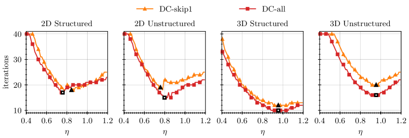
Figure 5: Sensitivity analysis of the measured iterations to convergence for the AMG preconditioned FGMRES solvers. Optimal parameter values, $\eta^{opt}$, are outlined in black (every fifth sample is marked).

Using the above-described parameter choices, we examine the convergence of FGMRES preconditioned with the monolithic AMG-based preconditioners and compare them against the Uzawa preconditioner for a range of problems and problem sizes. First consider the preconditioner based on the $\boldsymbol{\mathbb{P}}_{2}/\mathbb{P}_{1}$ AMG grid hierarchy, HO-AMG. For most problems, the HO-AMG preconditioner exhibits a slight growth in the iteration count as the problems are refined. We next evaluate the defect-correction (DC) approach based on the $\boldsymbol{\mathbb{P}}_{1}\text{iso}\kern 1.0pt\boldsymbol{\mathbb{P}}_{2}/\mathbb{P}_{1}$ discretization. Notice that DC-skip1, which effectively replaces the coarse grids of the HO-AMG hierarchy with an AMG hierarchy based on $K_{1}$, converges in 1–3 fewer iterations than the solvers based on HO-AMG. Since the DC-skip1 coarse grids are sparser than those of HO-AMG, the relative cost of the solution is slightly cheaper, as can be seen in the timing rows of Figure 6. However, the solution times are similar for HO-AMG and DC-skip1, because the relaxation cost at the finest level dominates the time to solution. For DC-skip0, relaxation on the $K_{0}$ system is skipped and replaced by relaxation on the $K_{1}$ system. The convergence of DC-skip0 suffers for all problem types, as seen in the top row of Figure 6. Despite having a lower cost per iteration than HO-AMG, the increase in the iteration count makes DC-skip0 less computationally effective than DC-skip1 and HO-AMG. This effect is particularly drastic for 3D problems, which can be seen in the last two columns of Figure 6. Although the solver based on DC-all converges in the fewest number of iterations for most problems, doubling the number of relaxation sweeps on fine grids (relaxing on both $K_{0}$ and $K_{1}$) results in significantly longer times to solution than for the HO-AMG approach. However, the relative difference in timing between DC-all and HO-AMG appears to diminish with larger problem sizes.

Figure 6: $\boldsymbol{\mathbb{P}}_{2}/\mathbb{P}_{1}$ solvers. Iterations to convergence (top), Relative time to solution (middle), and relative time per iteration (bottom). The relative timings are relative to the Uzawa solver.

The convergence and timing results in Figure 6, especially for DC-skip0 and DC-skip1, show conclusively that relaxation on the original problem ($K_{0}$) should not be skipped when designing a defect-correction type AMG preconditioner. Additional relaxation on the $K_{1}$ system may improve convergence further but at a higher computational cost. This conclusion is supported by the results from a GMG-based defect-correction approach published in [19].

In contrast, the Uzawa preconditioners exhibit slower convergence, requiring approximately 3–5 times more iterations to reach the convergence tolerance. This effect is particularly noticeable for 2D problems, where the iteration counts show significant growth. Comparing the time to convergence, we find that the monolithic AMG solvers outperform the Uzawa-based solvers by 20–50% for 2D problems. For structured 3D problems, the time to solution gap narrows to 20% with the fastest solver, DC-skip1. However, when dealing with unstructured 3D problems, the monolithic AMG-based solvers are generally slower than Uzawa. This difference in performance is partly due to the reduced number of iterations required for convergence in the Uzawa-based solver. The overall decrease in relative performance in 3D can be attributed to the substantial increase in Vanka patch sizes that must be solved at each level of the hierarchy. It is essential to explore strategies to reduce this computational cost to enhance the scalability of monolithic AMG solvers. Currently, this area represents an open field of research.

4.2 Preconditioning $\boldsymbol{\mathbb{P}}_{2}/\mathbb{P}_{1}^{disc}$ Systems

In this section, we evaluate the effectiveness of the defect-correction preconditioner for solving systems that have been discretized using $\boldsymbol{\mathbb{P}}_{2}/\mathbb{P}_{1}^{disc}$ elements on 2D structured and unstructured meshes. Preliminary numerical experiments (not reported here) showed that relaxation on all levels of the AMG hierarchy is needed to generate an efficient solver. The convergence data in Figure 8 uses the optimal damping parameter values tabulated in Table 3.

	Parameters
Mesh Type	$\omega_{0}^{opt}$	$\eta_{p}^{opt}$
Structured	0.78	2.68
Unstructured	0.58	4.00

Table 3: Optimal overweighting, $\eta_{p}^{opt}$, and damping, $\omega_{0}^{opt}$, parameters used in Scott-Vogelius, $\boldsymbol{\mathbb{P}}_{2}/\mathbb{P}_{1}^{disc}$, DC-all preconditioners.

We study the sensitivity of the FGMRES convergence rate to the parameter choices in DC-all by performing a parameter search on 3-level AMG hierarchies with at least a quarter million degrees of freedom on the finest $\boldsymbol{\mathbb{P}}_{1}\text{iso}\kern 1.0pt\boldsymbol{\mathbb{P}}_{2}/\mathbb{P}_{1}$ grid, for both structured and unstructured problems. We found that $\eta_{u}\approx 1$ produced the best convergence results, regardless of the values of $\omega_{0}$ and $\eta_{p}$, and so we fix $\eta_{u}^{opt}=1$. In order to determine the other parameters, we perform a 2D parameter scan. A two-dimensional heat map in Figure 7 shows the iteration counts for different choices of $\omega_{0}$ and $\eta_{p}$. The results indicate that the iteration counts are relatively insensitive to the choice of $\omega_{0}$ as long as they are between $0.5$ and $0.9$, and a similar trend is observed for the overweighting parameter, $\eta_{p}$, where values between $1.8$ and $5$ result in the best convergence. The optimal convergence regions for structured and unstructured problems are relatively close, but unstructured problems tend to perform best with smaller $\omega_{0}$ and larger $\eta_{p}$ values compared to structured problems. The optimal parameter choices are summarized in Table 3.

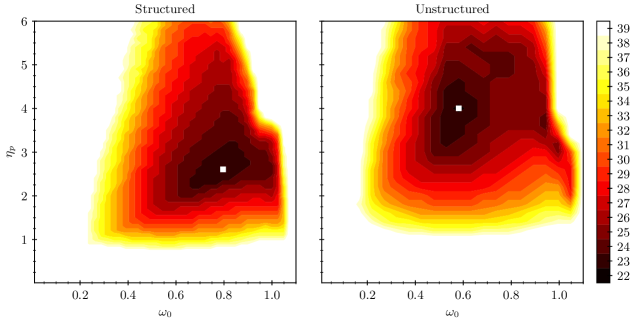
Figure 7: Sensitivity analysis of the measured iterations to convergence for the DC-all preconditioned FGMRES solvers. Optimal parameter values are marked with a white square.

Using the parameter choices described above, we now examine the convergence of these solvers across a range of problems and problem sizes. The iteration counts in Figure 8 show that the DC-all preconditioner converges, on average, in 27 iterations for structured domains and 23 iterations for unstructured domains, with the number of iterations increasing by one roughly with each order of magnitude increase in problem size. It is important to recall that the HO-AMG method does not converge on a significant number of the $\boldsymbol{\mathbb{P}}_{2}/\mathbb{P}_{1}^{disc}$ test problems and, so, it is revealing that DC-all converges on all test problems.

In contrast, the Uzawa preconditioners require around 4–5 times more iterations to reach convergence, and the iteration counts exhibit more significant growth. With each refinement of the problem (increasing the problem size by $2\times$), an additional 2–4 iterations are needed in Uzawa. Despite the substantial difference in iteration counts between Uzawa and DC-all, the overall runtime of Uzawa is only 20–30% slower for structured problems and 40–50% slower for unstructured problems. The improvement in performance of DC-all for unstructured problems can be attributed to the increased number of Uzawa iterations required for convergence compared to the decrease in DC-all iterations. It is important to note that each iteration of DC-all has a relative cost 3–4 times higher than a single iteration of Uzawa. We expect that the smaller number of iterations in DC-all will lead to additional performance improvement on parallel architectures, where the cost of synchronization operations, such as inner products, begins to grow due to communication overhead.

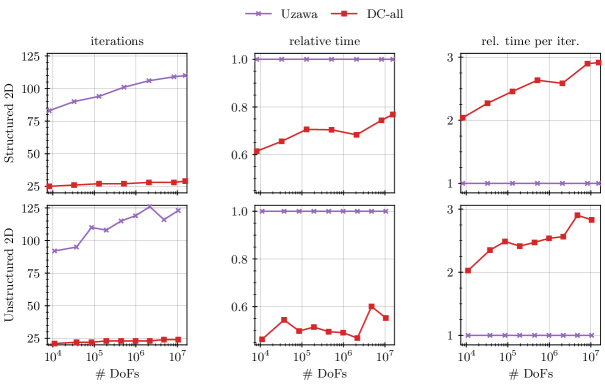
Figure 8: $\boldsymbol{\mathbb{P}}_{2}/\mathbb{P}_{1}^{disc}$ solvers. Relative time to solution(left), Iterations to convergence (middle) and relative time per iteration (right). The timings are relative with respect to Uzawa solver.

Our results demonstrate the effectiveness of the DC-all preconditioner for solving systems discretized using the $\boldsymbol{\mathbb{P}}_{2}/\mathbb{P}_{1}^{disc}$ discretizations. These findings validate the capabilities of our approach and offer valuable guidance for selecting optimal parameter values when utilizing the solver. Importantly, the comparison with the Uzawa method reveals the superiority of our approach in terms of iteration count and runtime.

5 Application Problems

We conclude by looking at the performance of the preconditioned FGMRES algorithms on two more realistic applications, pictured in Figure 9:

3D Artery: $\boldsymbol{\mathbb{P}}_{2}/\mathbb{P}_{1}$

This problem models fluid flow inside a 3D artery [52], discretized with unstructured tetrahedral elements. We used an STL file obtained from a luminal casting of a carotid artery bifurcation to generate a series of 3D meshes of increasing sizes [52]. The inflow boundary condition is imposed normal to the bottom left cross-section of the artery (see Figure 9(a)), and the outflow boundary conditions (Neumann) are imposed at the opposite two cross-sections, with zero Dirichlet boundary conditions on the velocity field on the other boundary faces of the domain.

2D Airfoil: $\boldsymbol{\mathbb{P}}_{2}/\mathbb{P}_{1}^{disc}$

This problem models the flow around an airfoil [52] in the center of the domain, with an adaptively refined 2D unstructured mesh of triangular elements. A parabolic inflow boundary condition is imposed along the left edge of the domain, while the homogeneous Neumann boundary condition is imposed on the outflow boundary at the right edge, with zero Dirichlet boundary conditions on the velocity field on all other boundary edges of the domain (including the inner airfoil).

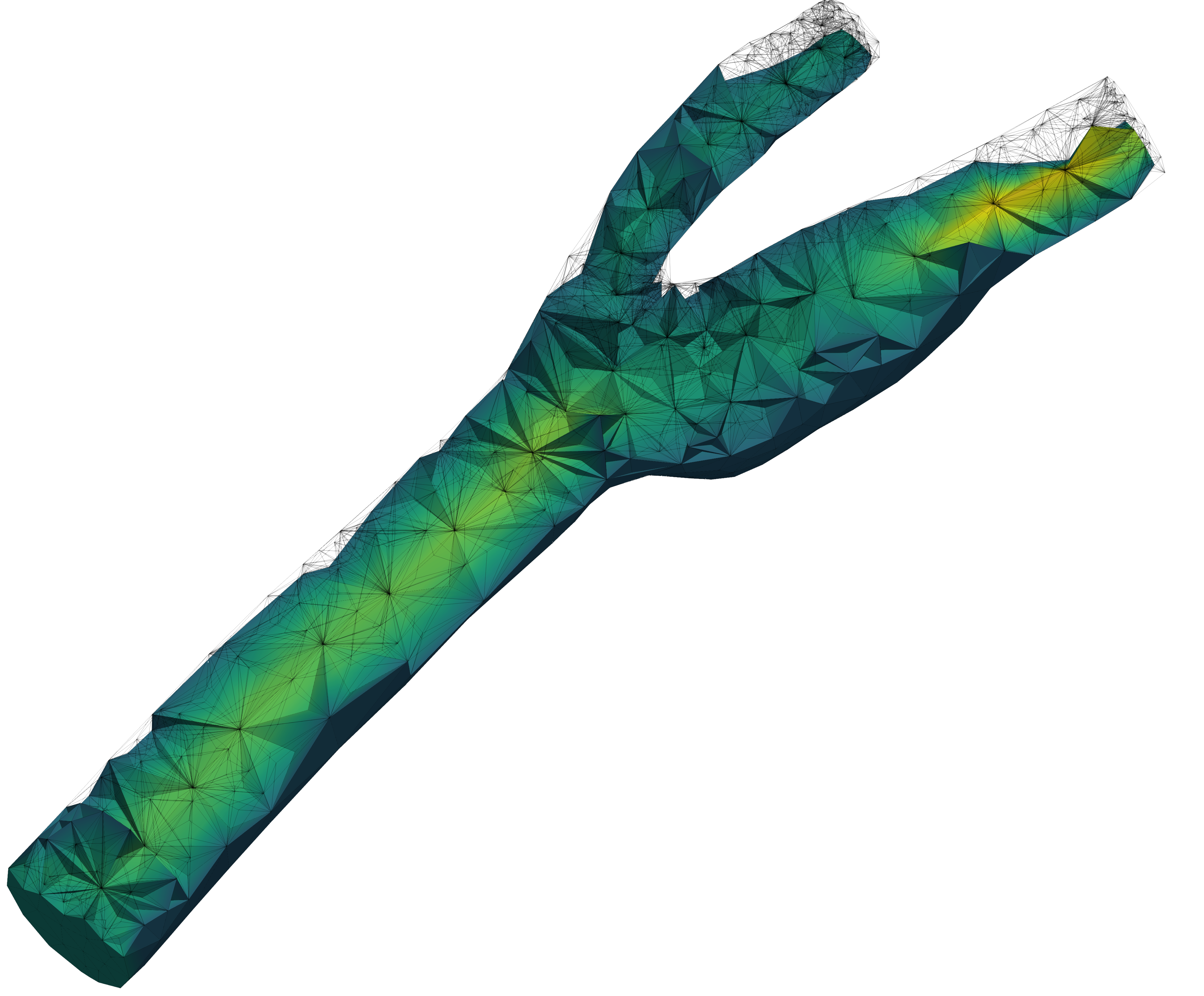
(a) 3D Artery: $\boldsymbol{\mathbb{P}}_{2}/\mathbb{P}_{1}$

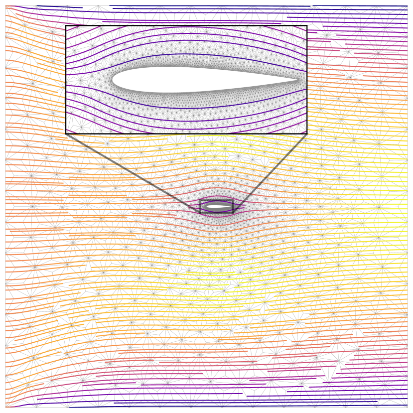
(b) 2D Airfoil: $\boldsymbol{\mathbb{P}}_{2}/\mathbb{P}_{1}^{disc}$

Figure 9: Test problems for Section 5

For all tests, we use the same convergence criteria and data collection approaches as discussed in Section 4. The convergence results reported in this section were collected with the same solver parameters described in Tables 2 and 3.

Figure 10 displays the iteration counts for multigrid preconditioned FGMRES, accompanied by the relative time per solution and iteration for each solver type. The top row of Figure 10 is associated with the 3D artery problem, discretized with the $\boldsymbol{\mathbb{P}}_{2}/\mathbb{P}_{1}$ element pair, whereas the bottom row corresponds to the 2D airfoil problem, discretized with $\boldsymbol{\mathbb{P}}_{2}/\mathbb{P}_{1}^{disc}$ elements.

Contrary to preceding numerical results sections, where we typically compare convergence timings against Uzawa preconditioner timings for the 3D problem, in this section, we compare DC-skip1’s timings with those of HO-AMG. This is primarily due to the fact that, in elongated domains, the pressure mass matrix does not serve as an effective preconditioner for the pressure Schur complement [13, 53]. Consequently, the Uzawa preconditioners’ convergence is significantly degraded for the 3D artery problem. For the problem sizes presented, the Uzawa preconditioners require 900–1500 iterations to converge, taking 20–30$\times$ longer than DC-skip1. Owing to the large discrepancies in iterations and timings, we omit these results and instead compare the performance of DC-skip1 in relation to HO-AMG.

Observing the 3D problem discretized with $\boldsymbol{\mathbb{P}}_{2}/\mathbb{P}_{1}$, we note that the defect-correction-based solver DC-skip1 converges with fewer (or an equivalent number of) iterations when compared to HO-AMG. However, the DC-skip1 solver runtime is approximately 13–25% faster than the HO-AMG-based solvers. This performance improvement is partially attributed to the reduced number of iterations, but it also stems from the fact that each iteration is 15–20% faster on average than one with HO-AMG. Even though HO-AMG and DC-skip1 share the same number of multigrid levels and perform an identical number of Vanka sweeps per iteration, DC-skip1 has superior speed. This can be credited to the $\boldsymbol{\mathbb{P}}_{1}\text{iso}\kern 1.0pt\boldsymbol{\mathbb{P}}_{2}/\mathbb{P}_{1}$ coarse grids being sparser than the $\boldsymbol{\mathbb{P}}_{2}/\mathbb{P}_{1}$ coarse grids. The sparser grids result in more compact algebraic Vanka patches, thereby requiring less computational work related to relaxation. Consequently, the DC-skip1 solver can accommodate larger-sized problems than HO-AMG on equivalent machines.

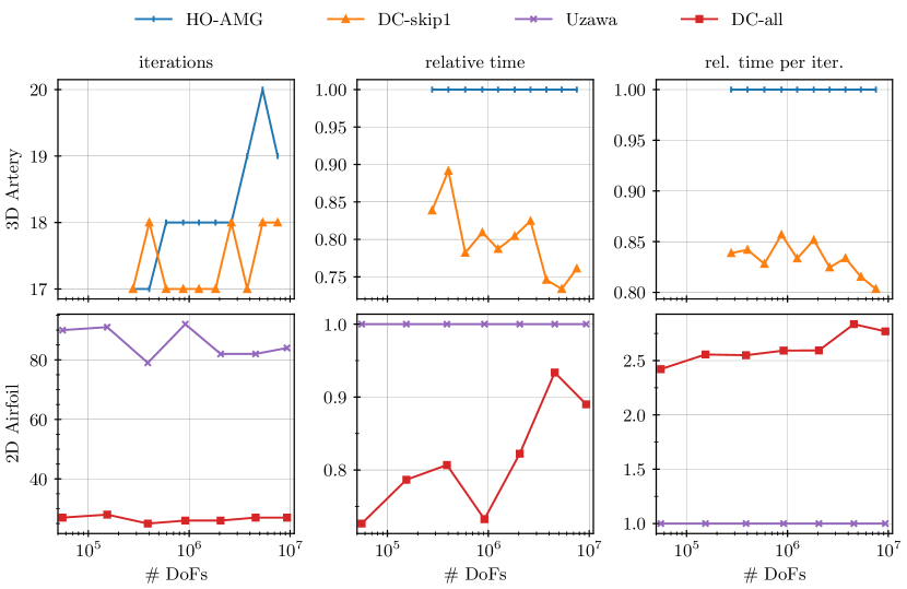
Figure 10: 3D $\boldsymbol{\mathbb{P}}_{2}/\mathbb{P}_{1}$ (top row) and 2D $\boldsymbol{\mathbb{P}}_{2}/\mathbb{P}_{1}^{disc}$ (bottom row) solvers. Iterations to convergence (left), Relative time to solution (middle), and relative time per iteration (right). Timings are relative to HO-AMG-based solver for top row and relative to Uzawa-based solver for bottom row.

For the 2D airfoil problem discretized with $\boldsymbol{\mathbb{P}}_{2}/\mathbb{P}_{1}^{disc}$ elements, we assess the performance of the low-order DC-all preconditioner against the Uzawa preconditioner. DC-all converges in a third of the iterations required by Uzawa and is 11–28% faster, depending on the problem size. Even with a 2.5–2.75$\times$ higher cost per iteration, DC-all’s significantly lower iteration counts yield faster overall convergence.

6 Conclusion

In this article, we present a novel algorithm designed to construct monolithic Algebraic Multigrid (AMG) preconditioners for the Stokes problem, utilizing a defect-correction approach predicated on the lower-order $\boldsymbol{\mathbb{P}}_{1}\text{iso}\kern 1.0pt\boldsymbol{\mathbb{P}}_{2}/\mathbb{P}_{1}$ discretization. We have shown the efficacy of this method for both $\boldsymbol{\mathbb{P}}_{2}/\mathbb{P}_{1}$ and $\boldsymbol{\mathbb{P}}_{2}/\mathbb{P}_{1}^{disc}$ discretizations. Moreover, the same methodology can be directly applied to the $\boldsymbol{\mathbb{P}}_{2}/\mathbb{P}_{1}$ discretization, generating a robust solver with a slightly higher cost per iteration compared to the low-order preconditioner. Both methods consistently demonstrate a relatively steady iteration count across various Stokes problems on structured and unstructured meshes in 2D and 3D. Impressively, the monolithic AMG preconditioners often match or even surpass the performance of inexact Uzawa preconditioners across a range of problems. The robustness of the monolithic AMG approach is particularly pronounced for the elongated-domain problem, which presents significant challenges in convergence for an inexact Uzawa-based solver.

There are several key ingredients to achieving the speedups realized in this work. We introduce an innovative approach for solution of the Vanka patch systems based on block factorization, offering reductions in storage and computation cost of up to 2x in 2D and 3x in 3D. We make use of an automatic relaxation parameter-picking method, Krylov-wrapping, which enhances the applicability of these multigrid methods to a broader range of problems without difficult parameter tuning. In scenarios where the relaxation and damping parameters still need to be calculated, such as in the case of the Scott-Vogelius discretization, we demonstrate that the optimal parameter choices remain relatively stable even when subjected to minor perturbations and can be efficiently computed using a coarse-parameter scan.

In future work, we aim to extend the $\boldsymbol{\mathbb{P}}_{1}\text{iso}\kern 1.0pt\boldsymbol{\mathbb{P}}_{2}/\mathbb{P}_{1}$-based defect-correction preconditioners to higher-order Taylor-Hood and Scott-Vogelius discretizations, utilizing a $p$-multigrid type approach. It is expected that the defect-correction preconditioners built on the $\boldsymbol{\mathbb{P}}_{1}\text{iso}\kern 1.0pt\boldsymbol{\mathbb{P}}_{2}/\mathbb{P}_{1}$ discretization may offer more significant advantages than the direct application of AMG to high-order systems with discontinuous bases, given the challenges inherent to such discretizations. In the context of higher-order solvers, efficient Vanka implementations on fine levels are set to become an increasingly vital component of the described defect-correction approach. Given the current trends in supercomputing, we anticipate that fine-level higher-order Vanka methods will be particularly amenable to efficient implementation on many-core systems due to their large stencils and highly-regular structure. Conversely, the coarse-level Vanka patches present more irregular shapes, making the design of efficient data structures a challenging task for future research.

References

- Elman et al. [2014] H. C. Elman, D. J. Silvester, A. J. Wathen, Finite elements and fast iterative solvers: with applications in incompressible fluid dynamics, Oxford University Press, USA, 2014.
- Benzi et al. [2005] M. Benzi, G. Golub, J. Liesen, Numerical solution of saddle point problems, Acta Numer. 14 (2005) 1–137.
- Adler et al. [2017] J. H. Adler, T. R. Benson, S. P. MacLachlan, Preconditioning a mass-conserving discontinuous Galerkin discretization of the Stokes equations, Numerical Linear Algebra with Applications 24 (2017) e2047.
- Farrell et al. [2021] P. E. Farrell, L. Mitchell, L. R. Scott, F. Wechsung, A Reynolds-robust preconditioner for the Scott-Vogelius discretization of the stationary incompressible Navier-Stokes equations, The SMAI journal of computational mathematics 7 (2021) 75–96.
- Brandt and Dinar [1979] A. Brandt, N. Dinar, Multigrid solutions to elliptic flow problems, in: S. Parter (Ed.), Numerical Methods for Partial Differential Equations, Academic Press, New York, 1979, pp. 53–147.
- Vanka [1986] S. P. Vanka, Block-implicit multigrid solution of Navier-Stokes equations in primitive variables, J. Comput. Phys. 65 (1986) 138–158.
- Linden et al. [1989] J. Linden, G. Lonsdale, B. Steckel, K. Stüben, Multigrid for the steady-state incompressible Navier-Stokes equations: a survey, in: 11th International Conference on Numerical Methods in Fluid Dynamics (Williamsburg, VA, 1988), volume 323 of Lecture Notes in Phys., Springer, Berlin, 1989, pp. 57–68.
- Braess and Sarazin [1997] D. Braess, R. Sarazin, An efficient smoother for the Stokes problem, Applied Numerical Mathematics 23 (1997) 3–19.
- Schöberl and Zulehner [2003] J. Schöberl, W. Zulehner, On Schwarz-type smoothers for saddle point problems, Numerische Mathematik 95 (2003) 377–399.
- Wabro [2004] M. Wabro, Coupled algebraic multigrid methods for the Oseen problem, Comput. Vis. Sci. 7 (2004) 141–151. doi:10.1007/s00791-004-0138-z.
- Wabro [2006] M. Wabro, AMGe—coarsening strategies and application to the Oseen equations, SIAM J. Sci. Comput. 27 (2006) 2077–2097. doi:10.1137/040610350.
- Metsch [2013] B. Metsch, Algebraic multigrid (AMG) for saddle point systems, Ph.D. thesis, Universitäts- und Landesbibliothek Bonn, 2013.
- Janka [2008] A. Janka, Smoothed aggregation multigrid for a Stokes problem, Comput. Vis. Sci. 11 (2008) 169–180.
- Prokopenko and Tuminaro [2017] A. Prokopenko, R. S. Tuminaro, An algebraic multigrid method for - mixed discretizations of the Navier-Stokes equations, Numerical Linear Algebra with Applications 24 (2017) e2109.
- Notay [2016] Y. Notay, A new algebraic multigrid approach for Stokes problems, Numerische Mathematik 132 (2016) 51–84.
- Notay [2017] Y. Notay, Algebraic multigrid for Stokes equations, SIAM Journal on Scientific Computing 39 (2017) S88–S111.
- Bacq and Notay [2022] P.-L. Bacq, Y. Notay, A new semialgebraic two-grid method for Oseen problems, SIAM Journal on Scientific Computing (2022) S226–S253.
- Bacq et al. [2023] P.-L. Bacq, S. Gounand, A. Napov, Y. Notay, An all-at-once algebraic multigrid method for finite element discretizations of Stokes problem, International Journal for Numerical Methods in Fluids 95 (2023) 193–214. doi:10.1002/fld.5145.
- Voronin et al. [2021] A. Voronin, Y. He, S. MacLachlan, L. N. Olson, R. Tuminaro, Low-order preconditioning of the Stokes equations, Numerical Linear Algebra with Applications (2021) e2426.
- Brandt [1984] A. Brandt, Multigrid techniques: 1984 guide with applications to fluid dynamics, GMD–Studien Nr. 85, Gesellschaft für Mathematik und Datenverarbeitung, St. Augustin, 1984.
- Niestegge and Witsch [1990] A. Niestegge, K. Witsch, Analysis of a multigrid Stokes solver, Appl. Math. Comput. 35 (1990) 291–303.
- John and Tobiska [2000] V. John, L. Tobiska, Numerical performance of smoothers in coupled multigrid methods for the parallel solution of the incompressible Navier-Stokes equations, International Journal For Numerical Methods In Fluids 33 (2000) 453–473.
- John et al. [2002] V. John, P. Knobloch, G. Matthies, L. Tobiska, Non-nested multi-level solvers for finite element discretisations of mixed problems, Computing 68 (2002) 313–341.
- Larin and Reusken [2008] M. Larin, A. Reusken, A comparative study of efficient iterative solvers for generalized Stokes equations, Numer. Linear Algebra Appl. 15 (2008) 13–34.
- Emami [2013] M. Emami, Efficient Multigrid Solvers for the Stokes Equations using Finite Elements, Master’s thesis, Lehrstuhl für Informatik 10 (Systemsimulation), Friedrich-Alexander-Universität Erlangen-Nürnberg, 2013.
- Gmeiner et al. [2016] B. Gmeiner, M. Huber, L. John, U. Rüde, B. Wohlmuth, A quantitative performance study for Stokes solvers at the extreme scale, J. Comput. Sci. 17 (2016) 509–521. doi:10.1016/j.jocs.2016.06.006.
- Adler et al. [2021] J. H. Adler, T. Benson, E. C. Cyr, P. E. Farrell, S. MacLachlan, R. Tuminaro, Monolithic multigrid for magnetohydrodynamics, SIAM J. Sci. Comput. 43 (2021) S70–S91.
- Heys et al. [2005] J. Heys, T. Manteuffel, S. F. McCormick, L. Olson, Algebraic multigrid for higher-order finite elements, Journal of Computational Physics 204 (2005) 520–532.
- Olson [2007] L. Olson, Algebraic multigrid preconditioning of high-order spectral elements for elliptic problems on a simplicial mesh, SIAM Journal on Scientific Computing 29 (2007) 2189–2209.
- Webster [2013] R. Webster, Stability of algebraic multigrid for Stokes problems, International Journal for Numerical Methods in Fluids 71 (2013) 488–505.
- Qin [1994] J. Qin, On the convergence of some low order mixed finite elements for incompressible fluids, Ph.D. thesis, The Pennsylvania State University, 1994.
- Zhang [2005] S. Zhang, A new family of stable mixed finite elements for the 3D Stokes equations, Mathematics of Computation 74 (2005) 543–554.
- Zhang [2008] S. Zhang, On the P1 Powell-Sabin divergence-free finite element for the Stokes equations, Journal of Computational Mathematics (2008) 456–470.
- Zhang [2011] S. Zhang, Quadratic divergence-free finite elements on Powell–Sabin tetrahedral grids, Calcolo 48 (2011) 211–244.
- John et al. [2017] V. John, A. Linke, C. Merdon, M. Neilan, L. G. Rebholz, On the divergence constraint in mixed finite element methods for incompressible flows, SIAM Review 59 (2017) 492–544.
- Case et al. [2011] M. A. Case, V. J. Ervin, A. Linke, L. G. Rebholz, A connection between Scott–Vogelius and grad-div stabilized Taylor–Hood FE approximations of the Navier–Stokes equations, SIAM Journal on Numerical Analysis 49 (2011) 1461–1481.
- Linke et al. [2011] A. Linke, L. G. Rebholz, N. E. Wilson, On the convergence rate of grad-div stabilized Taylor–Hood to Scott–Vogelius solutions for incompressible flow problems, Journal of Mathematical Analysis and Applications 381 (2011) 612–626.
- Ern and Guermond [2004] A. Ern, J.-L. Guermond, Theory and Practice of Finite Elements, volume 159 of Applied Mathematical Sciences, Springer-Verlag New York, 2004. doi:10.1007/978-1-4757-4355-5.
- Brandt and Yavneh [1993] A. Brandt, I. Yavneh, Accelerated multigrid convergence and high-Reynolds recirculating flows, SIAM Journal on Scientific Computing 14 (1993) 607–626.
- Chen et al. [2015] L. Chen, X. Hu, M. Wang, J. Xu, A multigrid solver based on distributive smoother and residual overweighting for Oseen problems, Numerical Mathematics: Theory, Methods and Applications 8 (2015) 237–252.
- Bell et al. [2022] N. Bell, L. N. Olson, J. Schroder, PyAMG: Algebraic multigrid solvers in python, Journal of Open Source Software 7 (2022) 4142. doi:10.21105/joss.04142.
- Vaněk et al. [1996] P. Vaněk, J. Mandel, M. Brezina, Algebraic multigrid by smoothed aggregation for second and fourth order elliptic problems, Computing 56 (1996) 179–196.
- Olson et al. [2010] L. N. Olson, J. Schroder, R. S. Tuminaro, A new perspective on strength measures in algebraic multigrid, Numerical Linear Algebra with Applications 17 (2010) 713–733.
- Voronin et al. [2021] A. Voronin, R. Tuminaro, L. N. Olson, S. MacLachlan, Algebraic Multigrid based on Low-order Systems, Technical Report, 2021. URL: https://www.sandia.gov/app/uploads/sites/210/2022/05/CSRI-2021-proceedings1.pdf#page=155.
- Farrell et al. [2021a] P. E. Farrell, M. G. Knepley, L. Mitchell, F. Wechsung, PCPATCH: Software for the topological construction of multigrid relaxation methods, ACM Trans. Math. Softw. 47 (2021a). doi:10.1145/3445791.
- Farrell et al. [2021b] P. E. Farrell, Y. He, S. P. MacLachlan, A local Fourier analysis of additive Vanka relaxation for the Stokes equations, Numerical Linear Algebra with Applications 28 (2021b) e2306.
- He and MacLachlan [2019] Y. He, S. P. MacLachlan, Local Fourier analysis for mixed finite-element methods for the Stokes equations, Journal of Computational and Applied Mathematics 357 (2019) 161–183.
- MacLachlan and Oosterlee [2011] S. P. MacLachlan, C. W. Oosterlee, Local Fourier analysis for multigrid with overlapping smoothers applied to systems of PDEs, Numer. Linear Alg. Appl. 18 (2011) 751–774.
- Brown et al. [2021] J. Brown, Y. He, S. P. MacLachlan, M. Menickelly, S. Wild, Tuning multigrid methods with robust optimization and local Fourier analysis, SIAM Journal on Scientific Computing 43 (2021) A109–A138.
- Rathgeber et al. [2016] F. Rathgeber, D. A. Ham, L. Mitchell, M. Lange, F. Luporini, A. T. T. Mcrae, G.-T. Bercea, G. R. Markall, P. H. J. Kelly, Firedrake: Automating the finite element method by composing abstractions, ACM Trans. Math. Softw. 43 (2016) 24:1–24:27. doi:10.1145/2998441.
- Kirby and Mitchell [2018] R. C. Kirby, L. Mitchell, Solver composition across the PDE/linear algebra barrier, SIAM Journal on Scientific Computing 40 (2018) C76–C98.
- Geuzaine and Remacle [2009] C. Geuzaine, J.-F. Remacle, Gmsh: A 3-D finite element mesh generator with built-in pre-and post-processing facilities, International Journal for Numerical Methods in Engineering 79 (2009) 1309–1331.
- Dobrowolski [2003] M. Dobrowolski, On the LBB constant on stretched domains, Mathematische Nachrichten 254 (2003) 64–67.