]Equal contribution as first author.

]Equal contribution as first author.

]Equal contribution as first author.

Supplementary Material for ”Generalization of Kirchhoff’s Law of Thermal Radiation: The Inherent Relations Between Quantum Efficiency and Emissivity”

I Explanation of the agreement between the generalized Kirchhoff’s law of thermal radiation and the scattering model

In the Generalized Kirchhoff’s law of thermal radiation, absorptivity describes the rate of excited electrons by a light source and is defined as $\alpha=1-\rho-\tau$, where $\rho$ and $\tau$ are the reflection and transmission coefficients, respectively. These electrons recombine radiatively or non-radiatively (defined by $QE$). The photoluminescence rate normalized by the pump, $PL_{n}$, and absorptivity are related as follows:

$$PL_{n}=\alpha\times QE$$

Following Eq. (8) from [1], we generalize the scattering coefficient $|s_{p}|^{2}$ as “everything that is exiting the material” in normalized units (including reflection, transmission, and $PL_{n}$):

$$|s_{p}|^{2}=\rho+\tau+\alpha\times QE=1-\alpha+\alpha\times QE$$ (S.1)

Following Eq. (9) from [1], for the absorptivity of the system and Eq. (12) from [1], substituting absorptivity and emissivity according to Kirchhoff’s law in equilibrium, we get:

$$\epsilon_{M}{}_{p}=\alpha_{M}{}_{p}=1-|s_{p}|^{2}$$

Using (S.1), this results in:

$$\epsilon_{M}{}_{p}=1-(1-\alpha+\alpha\times QE)=\alpha\times(1-QE)$$

In addition, Eq. (10) from [1] defines the linear superposition between scattered light and thermal emission. We show in our model the same linear superposition between PL (at 0K) and thermal emission.

II Boltzmann distribution of excited electron populations between two energy levels

The electron population in the three-level systems is described by Eq. (12a) and (12b) in the paper. For convenience, we present these equations here as well:

$$\frac{dn_{2}}{dt}= (n_{1}-n_{2})B_{r12}n_{ph12}-n_{2}\gamma_{r12}+(n_{1}-n_{2})B_{nr12}n_{pn12}-n_{2}\gamma_{nr12}+$$

$$(n_{3}-n_{2})B_{nr23}n_{pn23}+n_{3}\gamma_{nr23}$$

$$\frac{dn_{3}}{dt}= (n_{1}-n_{3})B_{r13}n_{ph13}-n_{3}\gamma_{r13}+(n_{1}-n_{3})B_{nr13}n_{pn13}-n_{3}\gamma_{nr13}-$$

$$(n_{3}-n_{2})B_{nr23}n_{pn23}-n_{3}\gamma_{nr23}$$

The last two terms in both equations are the non-radiative interactions between $n_{2}$ and $n_{3}$. $\gamma_{nr23}$ is the spontaneous non-radiative rate and $B_{nr23}=\gamma_{nr23}/DoS_{pn}$ is the stimulated non-radiative rate. The electronic levels interact with the phonon field, given by the equilibrium distribution $n_{pn23}=DoS_{pn}\left[exp\left(\frac{E_{23}}{k_{B}T}\right)-1\right]^{-1}$. Thus, we can rewrite these two last terms from Eq. (S.2) as:

$$(n_{3}-n_{2})B_{nr23}n_{pn23}-n_{3}\gamma_{nr23} = \gamma_{nr23}\left(\left[exp\left(\frac{E_{23}}{k_{B}T}\right)-1\right]^{-1}\left[n_{3}-n_{2}\right]+n_{3}\right)$$ (S.3)

$$= n_{3}\gamma_{nr23}\left(\left[exp\left(\frac{E_{23}}{k_{B}T}\right)-1\right]^{-1}\left[1-\frac{n_{2}}{n_{3}}\right]+1\right)$$

$$= n_{3}\gamma_{nr23}\left(1-\frac{\frac{n_{2}}{n_{3}}-1}{exp\left(\frac{E_{23}}{k_{B}T}\right)-1}\right)$$

For the case of dominant $\gamma_{nr23}$, at steady-state where $\frac{dn_{2}}{dt}=\frac{dn_{3}}{dt}=0$, the equality can be satisfied when these terms approach zero, leading to a Boltzmann distribution:

$$\frac{n_{2}}{n_{3}}\approx exp\left(\frac{E_{23}}{k_{B}T}\right)$$ (S.4)

III Analytical derivation of the generalized Kirchhoff law $\epsilon=\alpha\times(1-QE)$ for a two-level system

In Eq. (4), (5a) and (5b) in the paper, we derived the theoretical formalism for the populations of excited electrons and photons within a cavity with a two-level system. This formalism enables the calculation of the rate of photon emission from the cavity. We subsequently demonstrated that this emission consists of two mechanisms: quantum and thermal. For convenience, we have rewritten the equations and will now proceed to prove the primary equationn.

The rate of photons leaving the cavity:

$$n_{ph12}\Gamma_{out}=\Gamma_{out}\frac{n_{pump}\Gamma_{p}+NB_{nr12}n_{pn12}\frac{\gamma_{r}}{\gamma_{r}+\gamma_{nr}}}{\Gamma_{out}+NB_{r12}\left(1-\frac{\gamma_{r}}{\gamma_{r}+\gamma_{nr}}\right)}$$ (S.5)

Where:

$$L_{quantum}=\Gamma_{out}\frac{n_{pump}\Gamma_{p}}{\Gamma_{out}+NB_{r12}\left(1-\frac{\gamma_{r}}{\gamma_{r}+\gamma_{nr}}\right)}$$ (S.6a)

$$L_{thermal}=\Gamma_{out}\frac{NB_{nr12}n_{pn12}\frac{\gamma_{r}}{\gamma_{r}+\gamma_{nr}}}{\Gamma_{out}+NB_{r12}\left(1-\frac{\gamma_{r}}{\gamma_{r}+\gamma_{nr}}\right)}$$ (S.6b)

We refer to the ratio between the emitted (or reflected) and incoming photons into the cavity as the external quantum efficiency (EQE):

$$EQE\equiv\frac{n_{ph12}\Gamma_{out}}{n_{pump}\Gamma_{p}}=\Gamma_{out}\frac{1+\frac{NB_{nr12}n_{pn12}X}{n_{pump}\Gamma_{p}}}{\Gamma_{out}+NB_{r12}(1-X)}$$ (S.7)

Where $X=\frac{\gamma_{r}}{\gamma_{r}+\gamma_{nr}}$.

For any $\gamma_{r}$, we can examine the case of $QE\rightarrow 0$ where $\gamma_{nr}\gg\gamma_{r}$ and Eq. (S.7) is reduced to:

$$EQE_{(QE\rightarrow 0)}=\frac{1}{1+\frac{NB_{r12}}{\Gamma_{out}}}$$ (S.8)

EQE can be positive while $QE\rightarrow 0$ when the non-absorbed pump is reflected off the cavity. In this case, absorptivity is:

$$\alpha=1-EQE_{(QE\rightarrow 0)}=\frac{1}{1+\frac{\Gamma_{out}}{NB_{r12}}}$$ (S.9)

which is independent of $\gamma_{nr}$. At 0K, phonons are not thermally excited ($n_{pn12}\rightarrow 0$) and Eq. (S.7) becomes:

$$EQE_{(T\rightarrow 0)}=\frac{\Gamma_{out}}{\Gamma_{out}+NB_{r12}(1-X)}$$ (S.10)

The quantum efficiency is defined only at 0K, where the thermal emission vanishes, and it equals to the $EQE_{(T\rightarrow 0)}$ minus the photons reflected off the cavity, normalized to the pump absorbed photons. Therefore:

$$QE_{(T\rightarrow 0)} \equiv \frac{n_{ph12}\Gamma_{out}-(\alpha-1)n_{pump}\Gamma_{p}}{\alpha\cdot n_{pump}\Gamma_{p}}$$ (S.11)

$$= \frac{EQE_{(T\rightarrow 0)}}{\alpha}-\frac{1-\alpha}{\alpha}$$

$$= \frac{X}{1+\frac{NB_{r12}}{\Gamma_{out}}(1-X)}$$

In order to relate the EQE and the absorption coefficient, $\alpha$, we simplified Eq. (S.11):

$$\alpha(1-QE)=\frac{NB_{r12}(1-X)}{\Gamma_{out}+NB_{r12}(1-X)}$$ (S.12)

The rate of photons leaving the cavity when the pump is off is the thermal emission, Eq. (S.6b). After substituting $n_{pn}$ it can rewritten as:

$$n_{ph12}\Gamma_{out}=L_{thermal}=\Gamma_{out}f(T)\frac{NB_{nr12}DoS_{pn}X}{\Gamma_{out}+NB_{r12}(1-X)}$$ (S.13)

Considering the relations between the stimulated and spontaneous rates, we get:

$$B_{nr12}=B_{r12}\frac{1-X}{X}\cdot\frac{DoS_{ph}}{DoS_{pn}}$$ (S.14)

Substituting back into Eq. (S.13) yields:

$$L_{thermal}=\Gamma_{out}DoS_{ph}\cdot f(T)\frac{NB_{r12}(1-X)}{\Gamma_{out}+NB_{r12}(1-X)}$$ (S.15)

Using Eq. (S.12), the thermal emission becomes:

$$L_{thermal}=\Gamma_{out}\alpha\left(1-QE\right)DoS_{ph}\cdot f(T)$$ (S.16)

Comparing Eq. (S.16) with Plank’s law of thermal radiation: $L_{BB}=\epsilon\cdot DoS_{ph}\cdot f(T)$ , results in the prime equation:

$$\epsilon=\alpha\left(1-QE\right)$$ (S.17)

In this model, we assumed that the fundamental material parameters $\gamma_{r},\gamma_{nr},DoS_{ph},DoS_{pn}$ are temperature independent. Therefore, the emissivity, $\epsilon$, quantum efficiency and stimulated rates $B_{r12},B_{nr12}$ are also temperature independent.

IV Thermal emission spectra of all measured materials, 0.2%, 2% and %3 Er:YAG

See results in FIG. S.1.

(a)

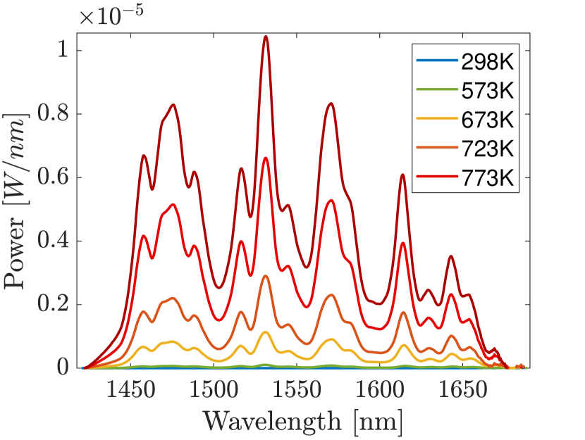
(b)

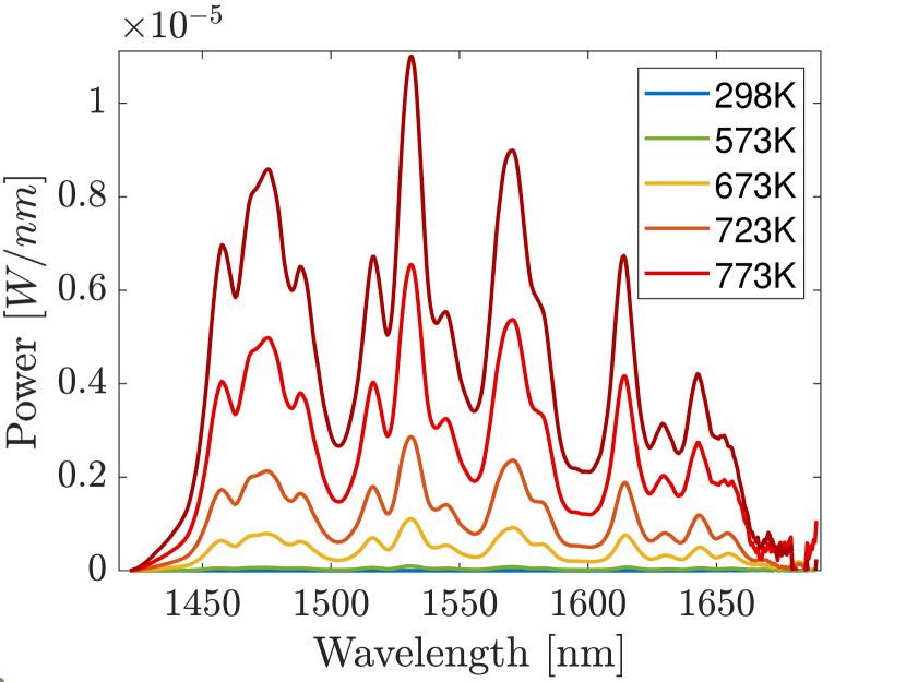
(c)

Figure S.1: Power spectra of thermal emissions of three Er:YAG concentrations in YAG crystals (0.2%, 2% and 3%).

V Normalization of the measured thermal spectrum

The experiment is performed in a free-space system, depicted in the paper. All samples are similarly aligned relative to the fiber. The numerical aperture and the distance at which the fiber is placed are such that the edges have no direct optical path to the fiber. Since Er:YAG has non-unity absorption at the measured spectra, we also account for the volume emission confined by the sample, presented in FIG. S.2.

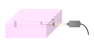
Figure S.2: Sample solid angle and emitting area.

Therefore, we normalize the measured thermal emission power with the solid angle of the fiber and measured emitting volume.

$$I_{emitted}[W]=I_{measured}[W]\cdot\frac{V_{sample}}{V_{cone}}\cdot\frac{4\pi}{\Omega_{fiber}}$$ (S.18)

Then $I_{emitted}$ is divided by the sample area and the $\pi$ solid angle to obtain the radiance:

$$R = \frac{I_{emitted}}{\pi A_{sample}}$$ (S.19)

$$= \frac{I_{measured}}{\pi A_{sample}}\cdot\frac{V_{sample}}{V_{cone}}\cdot\frac{4\pi}{\Omega_{fiber}}$$

$$= \frac{I_{measured}\cdot L}{\Omega_{fiber}\cdot V_{cone}}\left[\frac{W}{sr\cdot m^{2}}\right]$$

Here $V_{sample}=a\cdot L^{2}$ and $A_{sample}=4aL$ (upper and lower faces are reflecting), where $a$ is the sample’s height and $L$ is the sample’s length and width. In this case, the emissivity $\epsilon=\frac{R}{B.B}$ where $B.B$ denotes the black-body emission.

VI Absorptivity measurement and normalization

In FIG. 4 in the paper, we present the absorptivity averaged by the wavelength band in the range of 1450-1650 nm, measured and normalized inside an integrating sphere. For this, we first measure the directional absorptivity spectra of all the Er:YAG samples in the range of 850-1680 nm at room temperature (Cary 5000 UV-VIS), presented in FIG. 3(a).

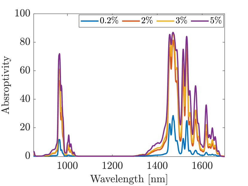
(a)

(b)

Figure S.3: Absorptivity of all Er:YAG samples. (a) The measured spectral absorptivity of all Er:YAG crystals. (b) The averaged absorptivity spectra, which are presented in (a), per band: 1450-1650 nm of all Er concentration samples.

We acquire the hemispherical absorptivity at the same spectral band by placing each sample with its silver cap inside an integrating sphere, as presented in FIG. S.4. To follow the experimental conditions of the emissivity experiment, where the sample radiates only in the peripherical directions, we place each sample on the silver plate holder, and cover it with the top silver plate, as presented by the inset in FIG. S.4. In this experiment, the sample is illuminated with the uniformly scattered laser diode, 1550 nm wavelength (Prefile, LDS 1550), from the walls of the integrating sphere, when the light beam hits first the baffle placed at the entrance of the sphere. The isotropic absorptivity is calculated as:

$$\alpha_{isotropic}\left(\lambda=1550[nm]\right)=\frac{I_{empty}-I_{sample\;in}}{I_{empty}}$$ (S.20)

where $I_{empty}$ and $I_{sample\;in}$ calibrated intensities at the diode emission wavelength when the sphere is empty and when the sample is placed inside the sphere, respectively. The ratio between the isotropic and directional absorptivity is the normalization factor by which the directional absorptivity at the measured spectrum is normalized.

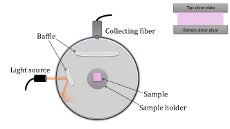
Figure S.4: Isotropic absorptivity measurement system. (a) presents schematically the measurement of the unabsorbed diode, where (b) illustrates the experimental system for measuring the diode. The placing of the sample between the bottom and top silver plates is presented in the inset of (a).

VII Emissivity independent of temperature

The generalized Kirchhoff’s law $\epsilon=\alpha\times(1-QE)$ is correct for any wavelength direction and $QE$. For simplicity in the paper, we develop the temperature evolution of the emission for $\gamma_{r}$ and $\gamma_{nr}$ to be temperature independent. We show that this assumption is true for the experiment with the Er:YAG samples. Fig. S.5 depicts the emissivity values of all measured samples. These values are the spectral sum of the emissivity $\sum_{\lambda}\epsilon(\lambda)$, obtained as the ratio of the thermal and black-body emissions at the range of 1450-1650 nm. We can see that the emissivity is, to a good approximation, constant, and therefore, independent of temperature.

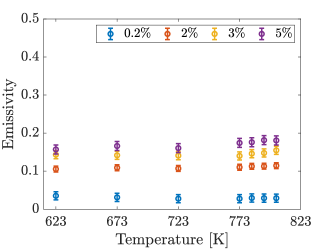
Figure S.5: Emissivity independent of temperature of all measured Er:YAG samples.

References

• Miller et al. [2017] D. A. Miller, L. Zhu, and S. Fan, Proceedings of the National Academy of Sciences 114, 4336 (2017).