Improving the Validity of Decision Trees as Explanations

Abstract

In classification and forecasting with tabular data, one often utilizes tree-based models. Those can be competitive with deep neural networks on tabular data and, under some conditions, explainable. The explainability depends on the depth of the tree and the accuracy in each leaf of the tree. Decision trees containing leaves with unbalanced accuracy can provide misleading explanations. Low-accuracy leaves give less valid explanations, which could be interpreted as unfairness among explanations. Here, we train a shallow tree with the objective of minimizing the maximum misclassification error across each leaf node. Then, we extend each leaf with a separate tree-based model. The shallow tree provides a global explanation, while the overall statistical performance of the shallow tree with extended leaves improves upon decision trees of unlimited depth trained using classical methods (e.g., CART) and is comparable to state-of-the-art methods (e.g., well-tuned XGBoost).

1 Introduction

In classification and forecasting with tabular data, one often utilizes axis-aligned decision trees (Payne and Meisel, 1977; Breiman et al., 1984). A prime example of a high-risk application of AI, where decision trees are widely used, is credit risk scoring (Mays, 1995; Thomas et al., 2017; Lessmann et al., 2015) in the financial services industry (Athey and Imbens, 2019). There, the relevant regulation, such as the Equal Credit Opportunity Act in the US (Equal Credit Opportunity Act, ECOA) and related regulation (European Commission, 2016a, b) in the European Union, bars the use of models that are not explainable (Rudin, 2019), which is often construed (Bracke et al., 2019; Dupont et al., 2020; Consumer Financial Protection Bureau, 2022; Gunnarsson et al., 2021) as requiring the use of decision trees. When studying the decision tree that a bank uses, one often focuses on ways that would make it possible to obtain a loan, and one would wish that the corresponding leaf of the decision tree had as high accuracy as possible.

In many other domains, the use of tree-based models has an equally long tradition. Consider, for example, judicial applications of AI such as the infamous Correctional Offender Management Profiling for Alternative Sanctions (COMPAS) (Brennan et al., 2009; Brennan and Dieterich, 2018; Courtland, 2018; Zhou et al., 2023), which is marketed as the “nationally recognized decision tree model”, or medical applications of AI (e.g., Rakha et al., 2014; London, 2019; Tjoa and Guan, 2020). It is hard to overstate the importance of high accuracy of any rule that a medical doctor or a judge may learn from a decision tree. In yet more domains, shallow decision trees are used (Bastani et al., 2017) to provide globally valid explanations of black-box classifiers, which is sometimes known (Bastani et al., 2017) as model extraction.

Shallow trees can indeed serve as global explanations for a classifier—or explainable classifiers per se—when each leaf is construed as a logical rule. Because various individuals or subgroups may deem various outcomes of importance, a fair explanation would have as high accuracy in each leaf of the decision tree as possible. The depth needs to be low in order for the rule explaining the decision in each leaf to remain comprehensible.

Similarly, one could argue that a decision tree can provide misleading explanations. To evaluate how valid or misleading the decision tree is, we suggest considering the minimal accuracy in any leaf of a tree (tree’s leaf accuracy). Indeed, a member of the public, when presented with the decision tree, may assume that each leaf of a decision tree can be construed as a logical rule. Consider, for example, the decision tree of Figure 1, based on the two-year variant of the well-known COMPAS (Brennan et al., 2009) dataset, which considers the binary classification problem of whether the individual would re-offend within the next two years. The left-most leaf may be interpreted as suggesting that for up to 3 prior counts and under 23 years of age, the defendant will re-offend within the next two years after release. However, the validity of this rule is somewhat questionable: the training accuracy in that leaf is 66.8%, while the test accuracy is 60% in that leaf. This suggests that 40% of defendants who meet these criteria will actually not re-offend within two years. For a more extreme example, see Figure 2, which shows two trees of similar overall accuracy for the pol(e) dataset. When optimizing for overall accuracy, the minimum test accuracy in one leaf can be as low as 57.1% (cf. the left tree in Figure 2). However, when maximizing the minimum training accuracy in one leaf, the minimum test accuracy in one leaf increases to 86.5% (cf. the right tree in Figure 2). One could argue that this improves the validity and fairness of the explanation provided by the tree.

Although a recent comparison of the statistical performance of gradient-boosted trees and deep neural networks by Grinsztajn et al. (2022) has shown that the state-of-the-art tree-based models can outperform state-of-the-art neural networks across a comprehensive benchmark of tabular data sets, for our decision trees, the low depth limits the overall accuracy. Therefore, one would like to improve the accuracy by “hybridizing” the tree, where the top, fixed-depth tree maximizing the leaf accuracy objective would explain as much of the variance as possible, given the depth. And below, tree-based models extending each leaf of the fixed-depth tree need not be interpretable but would improve the overall accuracy of the hybrid tree.

Here, we aim to introduce such hybrid trees and a two-step procedure for training these, to improve upon both the statistical performance and explainability of decision trees. In the first step of the procedure, we use mixed-integer programming (MIP) to train a shallow tree, with the objective of minimizing the maximum misclassification error across each leaf node and with constraints bounding the number of samples in each leaf node from below. Seen another way, we maximize the minimal accuracy in any leaf of a tree. In the second step, we train further tree-based models, which extend each leaf of the shallow tree. The shallow tree with the additional constraints on the accuracy in the leaves is easily explainable, while the overall statistical performance of these hybrid trees (Zhou and Chen, 2002) combining shallow trees and the extending tree-based models (which we call the hybrid-tree accuracy) improves upon the accuracy of decision trees of unlimited depth trained using classical methods (e.g., CART) and is comparable to state-of-the-art tree-based methods, such as the well-tuned XGBoost of Grinsztajn et al. (2022).

Figure 1: An example of the decision tree produced by proposed model for the COMPAS dataset, cf. Figure 3. The bold percentage shows the leaf accuracy in each leaf on out-of-sample data before applying the extending model. Below that, in regular font, we provide accuracy on training data.

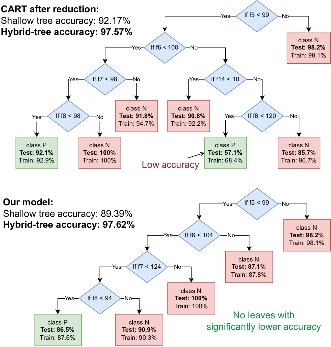
Figure 2: A comparison of decision trees produced by CART and our method for pol dataset. In each leaf, bold/regular percentage shows the leaf accuracy before extending it further on the test/training data set, respectively. Below the name of the model, we present the (hybrid-tree) accuracy of the hybrid/shallow tree in bold/regular font. The CART tree contains a leaf with a notably lower accuracy compared to the overall accuracy of the model. The explanation provided by this leaf is less valid. This makes the global explanation provided by the tree less fair. While model accuracies do not take this into account, the proposed measure of leaf accuracy does. The left and right trees have leaf accuracy on unseen data equal 57.1% and 86.5%, respectively.

Let us illustrate the statistical performance. Figure 3 shows that the accuracy of well-tuned XGBoost of Grinsztajn et al. on the two-year COMPAS (Brennan et al., 2009) test case exceeds 0.68. The accuracy of our shallow tree trained with the leaf-accuracy objective is below 0.65, which should not be surprising, considering the overall model accuracy is not the main objective. Nevertheless, by utilising the extending models in leaf nodes of the shallow tree, we can improve the accuracy very close to 0.68, which improves over both the accuracy of CART of the same depth alone (below 0.67) and CART of the same depth with extending models in leaf nodes of the tree (slightly above 0.67).

This performance is rather typical across the benchmark of Grinsztajn et al.. The proposed method outperforms CART with statistical significance, as detailed in Section 4.

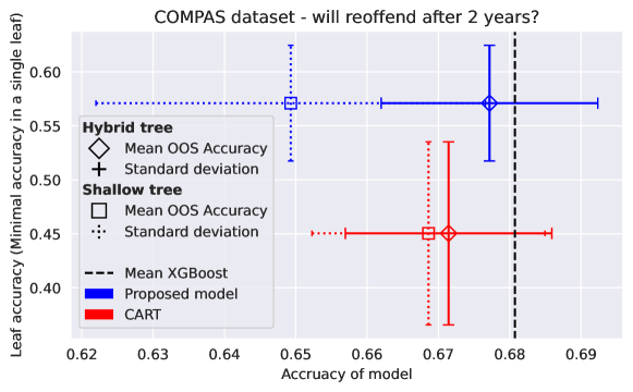
Figure 3: Performance on the COMPAS dataset: Mean statistical performance over 10 different train-test splits, evaluated in terms of model accuracy (horizontal axis) and leaf accuracy (vertical axis) for five variants of (hybrid) decision trees. The horizontal and vertical error bars are standard deviations across the 10 random runs. Notice that the proposed model has better interpretability compared to any standard decision tree and, once extended, accuracy comparable to a gradient-boosted tree.

Our contributions. We present:

• the challenge of fairness (or, equivalently, validity) of an explanation.

• leaf accuracy as a criterion for evaluating the validity and fairness of a classification tree as a global explanation. Leaf accuracy of decision tree $T$ is defined as follows:

  $$A_{L}(T)\coloneqq\min_{l\in\mathcal{L}(T)}\frac{1}{|X_{l}|}\sum_{(\boldsymbol{x},y)\in X_{l}}\llbracket y=C_{l}\rrbracket$$ (1)

  where $\mathcal{L}(T)$ is the set of leaf nodes of tree $T$, $X_{l}\subseteq X$ is the set of samples assigned to the leaf $l$, and $C_{l}$ is the decision class of the leaf $l$.

• a method for training decision trees that are optimal with respect to leaf accuracy, which is scalable across a well-known benchmark (Grinsztajn et al., 2022), despite its use of mixed-integer programming.

• benchmarking on tabular datasets (Grinsztajn et al., 2022) suggesting that the leaf accuracy can be improved by up to 18.41 percentage points, while suffering only a very modest drop (at most 2.76 percentage points across the benchmark) in overall model accuracy, compared to well-tuned XGBoost (Grinsztajn et al., 2022).

2 Related Work

Decision trees (Breiman et al., 1984) are among the leading supervised machine learning methods, where interpretability and out-of-sample classification performance is important. Random forests (Breiman, 2001) and gradient-boosting tree-ensemble approaches (Mason et al., 1999; Friedman, 2001) improve upon their statistical performance substantially while limiting the interpretability somewhat.

We are given $n$ samples $(x_{i1},\ldots,x_{ip},y_{i})$ with $p$ features each, for $i=1\ldots n$, and their classification $y_{i}\in[K]$ into $K$ classes. Let us denote sample $i$ by $\boldsymbol{x}_{i}=(x_{i1},\ldots,x_{ip})$. A decision tree sequentially splits a set of samples into two partitions: In each non-leaf node $t$, it splits the samples based on their values $x_{:j_{t}}$ of a particular feature $j_{t}\in[p]$ and a threshold $b_{t}$. (See Figure 1 for an illustration.) More recently, decision trees play an important role in explainable artificial intelligence (Arrieta et al., 2020; Burkart and Huber, 2021) and interpretable machine learning (Rudin et al., 2022).

Construction of an optimal axis-aligned binary decision tree is NP-Hard (Laurent and Rivest, 1976), and hence all known polynomial-time algorithms, such as CART (Breiman et al., 1984) produce suboptimal results, at least for some cases. Still, CART (Breiman et al., 1984), which utilizes the Gini diversity index and cross-validation in pruning trees, ranks among the leading algorithms (Wu et al., 2008) in machine learning. A decade later, Breiman suggested that boosting can be interpreted as an optimization algorithm (Breiman, 1998), leading to the development of gradient-boosted trees (e.g., Mason et al., 1999; Friedman, 2001). Their well-tuned variants (e.g., Chen and Guestrin, 2016; Ke et al., 2017; Prokhorenkova et al., 2018) are state-of-the-art polynomial-time algorithms for training decision trees. We refer to (Gorishniy et al., 2021; Grinsztajn et al., 2022) for comparisons against deep neural networks.

Bertsimas and Dunn (2017) and, independently others (Bessiere et al., 2009; Narodytska et al., 2018; Günlük et al., 2021), pioneered the use of exponential-time algorithms in the construction of decision trees. The integer-programming formulation of Bertsimas and Dunn suffers from some issues of scalability (Verwer and Zhang, 2019), but can be easily extended by the addition of further constraints, such as sparsity (Hu et al., 2019; Xin et al., 2022; Zhang et al., 2023), fairness (Verwer and Zhang, 2019; van der Linden et al., 2022), upper bounds on the number of leaves (Lin et al., 2020), incremental progress bounds (Lin et al., 2020), bounds on similarity of the support (Lin et al., 2020), a wide variety of privacy-related constraints, and in our case, accuracy in the leaves. Likewise, there are numerous extensions in terms of the objective (Lin et al., 2020), including F-score, AUC, and partial area under the ROC convex hull and, in our case, the leaf accuracy. Subsequently, the optimal decision trees have grown into a substantial subfield within machine learning research.

There have been several important proposals of alternative convex-programming relaxations for optimal decision trees: Dash et al. (2018) have demonstrated the use of an extended formulation in a column-generation (branch-and-price) approach; Zhu et al. (2020) have introduced another alternative formulation and a number of valid inequalities (cuts); Aghaei et al. (2020) have introduced yet another alternative formulation based on the maximum flow problem. Independently, Carreira-Perpinán and Tavallali (2018) suggested using non-linear optimization techniques, such as alternating minimization leading to much further research (Zantedeschi et al., 2021). We refer to Carrizosa et al. (2021); Nanfack et al. (2022) for overviews of mathematical optimization in the construction of decision trees.

Much recent research (e.g., Vidal and Schiffer, 2020; Demirović et al., 2022; van der Linden et al., 2022; Hua et al., 2022; Mazumder et al., 2022) has also focussed on improving the scalability of exponential-time algorithms for optimal decision trees by using branch-and-bound methods without relaxations in the form of convex optimization and, more broadly, dynamic programming. These approaches are sometimes seen as less transparent, as the mixed-integer formulation needs to be translated to the appropriate pruning rules or cost-to-go functions, which are less succinct, and the correctness of the translation can be non-trivial to verify. Nevertheless, Hua et al. (2022) have demonstrated the scalability of their method to a dataset with over 245,000 samples (utilizing less than 2000 core-hours), for example. On a benchmark of 21 datasets from the UCI Repository with over 7,000 samples, the algorithm can improve training accuracy by 3.6% and testing accuracy by 2.8% compared to the current state-of-the-art. This seems to validate the practical relevance of optimal decision trees.

3 Mixed-Integer Formulation

Mixed-Integer (Linear) Programming is a method of mathematical optimization similar to Linear Programming, with some of its variables limited to integer values. The goal is to maximize an objective function while satisfying a number of (linear) non-strict inequality constraints (Wolsey, 2021). Because of the global optimization capabilities, MIP enables our approach to not suffer from issues created by greedy top-down approaches like CART (e.g., Figure 2).

We build upon the Mixed-Integer Programming (MIP) formulation of optimal decision trees (Bertsimas and Dunn, 2017), changing the objective and adding novel constraints. The entire MIP formulation is presented in Figure 4.

$$\max\; Q$$ (2)

s. t. $$Q\leq\sum_{i=1}^{n}{S_{it}}+(1-l_{t}) \forall t\in\mathcal{T}_{L}$$ (3)

$$s_{it}\leq z_{it} \forall i\in[n],\;\forall t\in\mathcal{T}_{L}$$ (4)

$$r_{t}\leq s_{it}+(1-z_{it}) \forall i\in[n],\;\forall t\in\mathcal{T}_{L}$$ (5)

$$r_{t}\geq s_{it}+(z_{it}-1) \forall i\in[n],\;\forall t\in\mathcal{T}_{L}$$ (6)

$$l_{t}=\sum_{i=1}^{n}{s_{it}} \forall t\in\mathcal{T}_{L}$$ (7)

$$S_{it}\leq s_{it} \forall i\in[n],\;\forall t\in\mathcal{T}_{L}$$ (8)

$$S_{it}\leq\sum_{k=1}^{K}{Y_{ik}c_{kt}} \forall i\in[n],\;\forall t\in\mathcal{T}_{L}$$ (9)

$$S_{it}\geq s_{it}+\sum_{k=1}^{K}{Y_{ik}c_{kt}}-1 \forall i\in[n],\;\forall t\in\mathcal{T}_{L}$$ (10)

$$l_{t}=\sum_{k=1}^{K}{c_{kt}} \forall t\in\mathcal{T}_{L}$$ (11)

$$\boldsymbol{a}_{m}^{\mathsf{T}}\boldsymbol{x}_{i}\geq b_{m}-(1-z_{it}) \forall i\in[n],\;\forall t\in\mathcal{T}_{L},$$

$$\quad\qquad\forall m\in A_{R}(t)$$ (12)

$$\boldsymbol{a}_{m}^{\mathsf{T}}(\boldsymbol{x}_{i}+\boldsymbol{\epsilon})\leq \forall i\in[n],\;\forall t\in\mathcal{T}_{L},$$

$$\;\quad b_{m}+(1+\epsilon_{\max})(1-z_{it}) \quad\qquad\forall m\in A_{L}(t)$$ (13)

$$\sum_{t\in\mathcal{T}_{L}}{z_{it}}=1 \forall i\in[n]$$ (14)

$$z_{it}\leq l_{t} \forall i\in[n],\;\forall t\in\mathcal{T}_{L}$$ (15)

$$\sum_{i=1}^{n}{z_{it}}\geq N_{\min}l_{t} \forall t\in\mathcal{T}_{L}$$ (16)

$$\sum_{j=1}^{p}{a_{jt}}=1 \forall t\in\mathcal{T}_{B}$$ (17)

$$0\leq b_{t}\leq 1 \forall t\in\mathcal{T}_{B}$$ (18)

$$z_{it},l_{t}\in\{0,1\} \forall i\in[n],\;\forall t\in\mathcal{T}_{L}$$ (19)

$$a_{jt}\in\{0,1\} \forall j\in[p],\;\forall t\in\mathcal{T}_{B}$$ (20)

$$c_{kt}\in\{0,1\} \forall k\in[K],\;\forall t\in\mathcal{T}_{L}$$ (21)

$$0\leq Q,r_{t},S_{it},s_{it}\leq 1 \forall i\in[n],\;\forall t\in\mathcal{T}_{L}$$ (22)

Figure 4: The complete MIP formulation of training the shallow tree maximizing the minimum accuracy across all leaf nodes and constraining the number of samples per leaf node. The constraints (11 – 21) are taken from the optimal decision trees of Bertsimas and Dunn (2017), and the remaining constraints (3 – 10) and (22), together with a different objective function (2), are parts of our extensions. We use $[n]$ notation to represent the set of integers $\{1,2,3,\ldots,n\}$. An overview table of the variables and parameters is in the Appendix (Table 3).

Base model

As in the original optimal decision trees (Bertsimas and Dunn, 2017), we have $n$ samples with $p$ features each. Every point has one of $K$ classes, which is represented in the formulation by a binary matrix $Y$ such that $Y_{ik}=1$ $\iff$ $y_{i}=k$. All tree nodes are split into two disjoint sets, $\mathcal{T}_{B}$ and $\mathcal{T}_{L}$, which are sets of branching nodes and leaf nodes, respectively. Variable $\boldsymbol{a}_{t}$ is a binary vector of dimension $p$ that selects a feature $j$ to be used for decisions in node $t$. It holds that $a_{jt}=1\iff j$ is the selected feature in node $t$. $b_{t}$ is then the value of the threshold. We assume all data are normalized to $[0,1]$ range.

Equations (11–21) capture the original model of Bertsimas and Dunn (2017), wherein:

• Binary variable $c_{kt}$ is equal to 1 if and only if leaf node $t$ predicts class $k$ to data.

• Binary variable $l_{t}$ is equal to $1$ if and only if there is any point classified by the leaf node $t$.

• Binary variable $z_{it}$ is equal to $1$ if and only if point $x_{i}$ is classified by leaf node $t$.

The only modification to the original formulation is the omission of a binary variable $d_{t}$ that decided whether a certain branching node is used. This introduced a flaw in the original formulation (Bertsimas and Dunn, 2017), which led to invalid trees, so we decided against using it. We assume it to always be $1$ instead. To prune redundancies, we introduce a process of tree reduction described in Section 3.

Equations (12) and (13) implement the split of samples to leaf node $t$ using disjoint sets $A_{R}(t)$ and $A_{L}(t)$, containing nodes to which the leaf $t$ is on the right or on the left, respectively. Since we cannot use strict inequality, we use $\boldsymbol{\epsilon}$, a $p$-dimension vector of the smallest increments between two distinct consecutive values in every feature space (Bertsimas and Dunn, 2017):

$$\epsilon_{j}=\min\left\{x_{j}^{(i+1)}-x_{j}^{(i)}\Big{\rvert}x_{j}^{(i+1)}\neq x_{j}^{(i)},\forall i\in\{1,\ldots,n-1\}\right\}$$

where $x_{j}^{(i)}$ is the $i$-th largest value in the $j$-th feature, $\epsilon_{\max}$ is the highest value of $\epsilon_{j}$ and serves as a tight big-M bound.

Finally, Equation (16) bounds the number of points ($N_{\min}$) in a single leaf from below.

MIP extensions

In the original optimal decision trees (Bertsimas and Dunn, 2017), the objective is to minimize total misclassification error. Instead, we wish to maximize the leaf accuracy. Because a single sample usually contributes differently to accuracy at different leaves, we need to introduce multiple new variables to track the accuracy in each leaf:

• variable $s_{it}$ represents the potential accuracy that sample $\boldsymbol{x}_{i}$ has in leaf $t$. It takes values in the range $[0,1]$ and must sum to $1$ when summing across all samples assigned to leaf $t$. This is ensured by setting the value to $0$ for all points that are not assigned to the leaf $t$ in constraint (4). The sum of $1$ is enforced in constraint (7) for non-empty leaves. Empty leaves do not have non-zero $s_{it}$ values for any $i$ and thus could not sum to 1.

• reference accuracy variable $r_{t}$ serves as a common variable to which all accuracy contributions are equal. This is, of course, required only for points assigned to the leaf $t$. This is enforced in (5) and (6).

• variable $S_{it}$ represents the true assignment of accuracy given by the sample. That is achieved by setting it to $0$ for misclassified points using constraint (9) and by setting it equal to $s_{it}$ otherwise by constraints (8) and (10).

• variable $Q$ is our objective and represents the leaf accuracy of the tree. Equivalent to $A_{L}(T)$ defined in Equation (1), it is the lowest achieved accuracy across all non-empty leaves as per constraint (3). For empty leaves, this constraint will be trivially satisfied since $Q$ cannot take value higher than $1$ anyway.

Tree reduction

After the optimizer of the mixed-integer program is obtained, empty leaves are pruned to obtain the resulting unbalanced tree. Furthermore, to account for suboptimal solutions obtained when the solver is run with a strict time limit, each pair of sibling leaves classified in the same class is merged. This is performed recursively until no further action can be performed. This leads to no loss in model accuracy and oftentimes leads to an improvement in leaf accuracy, given the fact that we consider the minimum over all leaves.

Tree extension

Finally, we extend the remaining leaves with new tree-based models to improve hybrid-tree accuracy that is comparable to the best-performing models. In particular, we used XGBoost as the extending model since it was the best-performing model on the used benchmark (Grinsztajn et al., 2022). We trained a separate model for each leaf of the shallow tree after the aforementioned reduction. The hyperparameters of the models were tuned using 50 iterations of a Bayesian hyperparameter search with 3-fold cross-validation in each leaf. In experiments, we reduce and extend trees generated by other methods (OCT, CART) in the same way.

4 Numerical results

We have implemented the method in Python, and all code and results are provided in the Supplementary material. We will release them under an open-source license on GitHub once the paper has been accepted. The hyperparameters have been chosen as follows:

• The shallow trees have been trained using the formulation in Figure 4 with depth limited to four since that is a reasonable threshold for interpretability (e.g., printability on an A4 page, similar to Figure 1) and for not diluting the dataset to small parts that would impede the ability to train the extending models.

• To further support this, we set the minimal amount of points in a leaf ($N_{\min}$) to 50.

• MIPFocus and Heuristics hyperparameters were set to 1 and 0.8, respectively, to focus on finding feasible solutions in the search since that leads to the fastest improvements of the solution. However, our experiments in Appendix A.3 show that default MIP solver hyperparameters perform similarly.

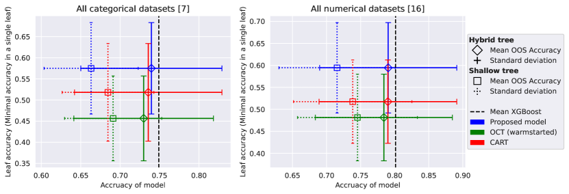
Figure 5: Results on out-of-sample data. The plot shows a significant increase in leaf accuracy when using our method, significantly improving the validity of the explanations provided. It also shows an increase in model accuracy when extending the models with XGBoost models in leaves. The results of the OCT model serve to compare to the model we built upon.

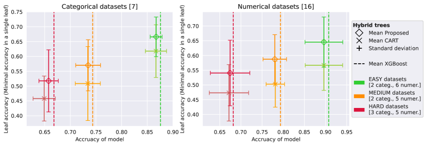
Figure 6: Results on out-of-sample data on all classification datasets from the tabular benchmark partitioned into 3 categories by complexity. In square brackets are the numbers of datasets belonging to each partition. This plot shows that our method, when extended in leaves, does not significantly decrease overall performance compared to pure XGBoost while sometimes improving upon accuracy obtainable by extended CART. And it does so consistently for datasets of varying complexity.

We performed our experiments on the benchmark of Grinsztajn et al., which contains datasets for both regression and classification. The benchmark consists of real datasets, on which tree-based models are the best performing, making it a good fit for our purpose. Since our implementation considers only classification, we consider only classification datasets. Grinsztajn et al. (2022) divide the datasets into numerical datasets and datasets with some categorical features. We follow this distinction and present results on both kinds of datasets separately. We also follow the suggestion of Grinsztajn et al. to perform 10 different train-test splits with at most 10,000 data points or 80% of total data points (whichever is lower) for training across all datasets. That is, each model has been trained on each dataset 10 times, with different seeds for data splits. The training used 80% of all data points or 10,000 data points, whichever is lower, while the remaining 20% of the dataset has been used as the test set for evaluating the model accuracy and leaf accuracy $A_{L}(T)$—see Equation (1). All MIP formulations of our shallow tree were warmstarted using a CART solution trained on the same data with default scikit-learn parameters, except for maximal depth and a minimal number of samples in a leaf, which were set to 4 and 50, respectively.

We performed all experiments on an internal cluster with sufficient amounts of memory. Each run of the MIP solver has been limited to 8 hours on 8 cores of AMD Epyc 7543, totaling 64 core-hours per split of a dataset. The extension part takes, on average, around 1 additional 3 core-hours per split. This totals around 15,500 core-hours for the entire classification part of the tabular benchmark and one configuration of hyperparameters. Training each dataset requires between 15 and 95 GB of working memory; details are provided in the Appendix (Figure 9). In this setting, the Gurobi solver closes the MIP Gap to around 60% on average. Further discussion of MIP Gaps is in Appendix A.3. Still, even after 1 hour of computation, the proposed model outperforms CART; see Figure 10(c) in Appendix.

	Data Type	Min	Mean ($\pm$ std)	Max
Compared to CART
Leaf Accuracy	categorical	$-0.0142$	$0.0569\pm 0.0533$	$0.1206$
	numerical	$-0.0061$	$0.0770\pm 0.0556$	$0.1841$
Hybrid-tree Acc.	categorical	$-0.0078$	$0.0040\pm 0.0071$	$0.0147$
	numerical	$-0.0244$	$0.0004\pm 0.0082$	$0.0087$
Compared to XGBoost
Hybrid-tree Acc.	categorical	$-0.0228$	$-0.0095\pm 0.0064$	$-0.0036$
	numerical	$-0.0276$	$-0.0108\pm 0.0076$	$0.0005$

Table 1: Improvements in mean accuracy on datasets between our model and comparable models. Data is computed by subtracting the mean accuracy of CART or XGBoost, respectively, on each dataset from the mean accuracy of our model. In the first two rows, we compare the leaf accuracy of our model to CART. In the middle two rows, we compare the model accuracy of the hybrid trees with CART extended in the same way. In the last two rows, we compare our extended hybrid-tree model to the mean XGBoost model trained on the same dataset.

We compare our method of training classification trees to CART, as it is by far the most common. All experiments used the scikit-learn implementation of CART, also utilizing the option of cost complexity pruning. The hyperparameters for CART were optimized using Bayesian hyperparameter optimization for 100 iterations using 5-fold cross-validation. Hyperparameter search space was notably constrained only by fixing a maximal depth to 4 and a minimal number of samples in leaves to 50, ensuring comparability to our shallow trees. In comparison to unconstrained depth CART and CART with optimized lower bound on the number of samples in a leaf, our model interestingly fared even better. See Appendix A.9 for details. The entire optimization of CART with the extensions of the leaves took around 500 core-hours for the entire benchmark.

The XGBoost results are taken from the authors of the paper introducing the benchmark, which suggests 20,000 core-hours have been spent producing these. (Grinsztajn et al., 2022)

Figure 5 shows the average performance (model accuracy and leaf accuracy) over categorical and numerical datasets. We include the comparison to optimal classification trees (OCT) (Bertsimas and Dunn, 2017) since it is the formulation we built on. The OCT model is warmstarted the same way as the proposed model and has the worst performance. The proposed model improves the leaf accuracy by 7.09 percentage points on average compared to CART.

Figure 6 shows again the average performance separately on categorical and numerical datasets divided into three groups by complexity. The measure of complexity is based on the performance of XGBoost provided by the authors of the benchmark. The thresholds of partitions are 0.7 and 0.8 for datasets containing categorical features and 0.75 and 0.85 for datasets with only numerical features. The thresholds were selected in order to separate too easy and too hard datasets, which make the plots less informative, and to explore behavior on datasets with varying inner complexity. We see that the proposed method always significantly improves the leaf accuracy compared to CART.

Table 1 quantifies the differences numerically. Proposed models have worse accuracy by about 1 percentage point on average when compared to the uninterpretable, best-performing state-of-the-art models (XGBoost). Compared to CART, a different training process of the same model, our approach slightly improves the model accuracy, but more importantly, it improves the leaf accuracy.

Statistical significance

Demšar (2006) summarizes statistical tests used for the comparison of algorithms on multiple datasets. Compared to CART, the proposed method has better leaf accuracy and better hybrid-tree accuracy on a substantial majority of datasets. Using the basic sign test (Demšar, 2006), both results are statistically significant with $p<0.05$. Using the Wilcoxon signed-rank test, we reject the null hypothesis that CART performs better than the proposed method with high confidence ($\alpha\leq 0.01$ for leaf accuracy and $\alpha\leq 0.05$ for hybrid-tree accuracy).

For more insight into the results, refer to Appendix A.7.

5 Conclusions and Limitations

We have identified an important problem of the fairness and validity of a tree as an explanation and have shown that contemporary tree-based models do leave room for improvement in terms of fairness. The use of hybrid trees, where the top is constructed with the goal of maximizing leaf accuracy, offers multiple benefits.

First, it ensures better validity of every explanation provided, improving the leaf accuracy by around 7 percentage points on average across the benchmark of tabular datasets (Grinsztajn et al., 2022).

Second, the hybrid-tree accuracy with tree-based models extending the leaves improves over the accuracy of shallow trees constructed using integer programming as well as hybrid trees, where the shallow tree is obtained using CART.

Finally, it is easy to extend to further constraints, such as shape constraints, in the top tree. Overall, we hope that the proposed approach may lead to improving the validity and fairness of decision trees as explanations.

Limitations

The hybrid-tree model aims to strike a balance between global explainability and model accuracy. The extending models, while improving the accuracy, bar the use of the shallow tree as an explanation in cases when the extending model changes the decision of the shallow tree. To explain such decisions, it requires the use of other explanation methods. That being said, the shallow tree can explain a significant part of the data while ensuring the global explanation provided is fair and valid for all paths from the root.

The proposed approach shares some of the limitations of the original optimal decision trees (Bertsimas and Dunn, 2017). Notably, the algorithms we utilize for solving mixed-integer programming problems scale exponentially in the number of decision variables. Having said that, depth-4 trees suffice to match state-of-the-art methods in terms of accuracy when additional tree-based models extend from the leaves, which makes exponential time algorithms sufficiently fast in practice. Furthermore, all recently proposed methods (e.g., Vidal and Schiffer, 2020; Demirović et al., 2022; van der Linden et al., 2022; Hua et al., 2022; Mazumder et al., 2022) improving the scalability can be applied, in principle.

Appendix A Appendix

In the Supplementary material, we provide the source code, complete results in .csv files, and a Jupyter notebook with example tests. All will be publicly available once the paper is accepted. Here, we present the results of further tests performed and describe ablation analyses and provide further details about the results already presented.

A.1 Datasets

We used the classification part of the data sets from the mid-sized tabular data put together by Grinsztajn et al. [2022]. The datasets, with their properties, are listed in Table 2. Training sets contained 80% of the total amount of samples truncated to at most 10,000 samples. This constraint affects 16 of the 23 total datasets, although some only marginally. The affected datasets have their number of samples in Table 2 in bold. The remaining 20% of the samples were the testing dataset. We used 10 random seeds that determined the train-test splits of each dataset and fixed the randomness in the training process. The seeds were namely integers 0 to 9.

Additionally, datasets are either categorical or numerical. Categorical are those that contain at least one categorical feature. Numerical datasets have no categorical features. Four numerical datasets are the same as categorical datasets but with their categorical features removed (covertype, default-of-credit-card-clients, electricity, eye_movements). Only datasets without missing features and with sufficient complexity are included in the benchmark. For more details on the methodology of dataset selection, we refer to the original paper [Grinsztajn et al., 2022].

categorical datasets	# of samples	# of features	# of classes
albert	58252	31	2
compas-two-years	4966	11	2
covertype	423680	54	2
default-of-credit-card-clients	13272	21	2
electricity	38474	8	2
eye_movements	7608	23	2
road-safety	111762	32	2
numerical datasets	# of samples	# of features	# of classes
bank-marketing	10578	7	2
Bioresponse	3434	419	2
california	20634	8	2
covertype	566602	32	2
credit	16714	10	2
default-of-credit-card-clients	13272	20	2
Diabetes130US	71090	7	2
electricity	38474	7	2
eye_movements	7608	20	2
Higgs	940160	24	2
heloc	10000	22	2
house_16H	13488	16	2
jannis	57580	54	2
MagicTelescope	13376	10	2
MiniBooNE	72998	50	2
pol	10082	26	2

Table 2: Listed classification datasets of the tabular benchmark. Train sets contained 80% of the total amount of samples truncated to at most 10 000 samples. 16 datasets affected by this have their number of samples in bold.

A.2 MIP formulation description

We provide Table 3 with short descriptions of the parameters and variables in the MIP formulation of the proposed model from Figure 4.

Symbol		Explanation	Size
Params	$Y_{ik}$	Equal 1 for true class of a sample	$n\times K$
	$\boldsymbol{x}_{i}$	Input samples	$n\times p$
	$\boldsymbol{\epsilon}$	Minimal change in feature values	$p$
	$\epsilon_{\max}$	Maximal value of $\boldsymbol{\epsilon}$	$1$
	$N_{\min}$	Minimum of samples in a leaf	$1$
	$\mathcal{T}_{L}$	Set of leaf nodes	$2^{d}$
	$\mathcal{T}_{B}$	Set of decision (branching) nodes	$2^{d}-1$
	$A_{L}(t)$	Ancestors of leaf $t$ that decide left	$\leq d-1$
	$A_{R}(t)$	Ancestors of leaf $t$ that decide right	$\leq d-1$
Variables	$Q$	Tree’s leaf accuracy	1
	$s_{it}$	Accuracy potential of $\boldsymbol{x}_{i}$ in leaf $t$	$n\times 2^{d}$
	$S_{it}$	Accuracy contribution of $\boldsymbol{x}_{i}$ in leaf $t$	$n\times 2^{d}$
	$r_{t}$	Reference accuracy for $s_{:t}$	$2^{d}$
	$z_{it}$	Assignment of $\boldsymbol{x}_{i}$ to leaf $t$	$n\times 2^{d}$
	$l_{t}$	Non-emptiness of leaf $t$	$2^{d}$
	$c_{kt}$	Assignment of class $k$ to leaf $t$	$K\times 2^{d}$
	$a_{jt}$	1 if deciding on feature $j$ in node $t$	$p\times(2^{d}-1)$
	$b_{t}$	Decision threshold in node $t$	$2^{d}-1$

Table 3: Description of MIP symbols used in the proposed formulation in Figure 4. Parameter $n$ refers to the number of samples, $K$ is the number of classes, $p$ is the number of features, and $d$ is the depth of the tree.

A.3 MIP Solver

We have utilized Gurobi optimizer as a MIP solver. Although the solver makes steady progress towards global optimality, the road there is lengthy. Figure 7(b) shows the progress of the MIP Gaps during the 8-hour optimization averaged over all datasets. For a detailed, per-dataset view, see Figure 8. The solution is still improving, albeit rather slowly, after 8 hours. The narrowing of the MIP gap is achieved only by finding better feasible solutions. This lack of improvement of the objective bound might have been affected by our hyperparameter settings which focused on finding feasible solutions and heuristic search. However, tests with default parameters did not improve the best bound either.

Default hyperparameters of Gurobi solver

The performance of the Gurobi optimizer depends on the choice of hyperparameters. For the sake of simplicity, we have considered only two sets of parameters. To measure the performance change of our choice of (hyper)parameters, we ran a test with the default value of the MIPFocus parameter and a test with the default value of the Heuristics parameter.

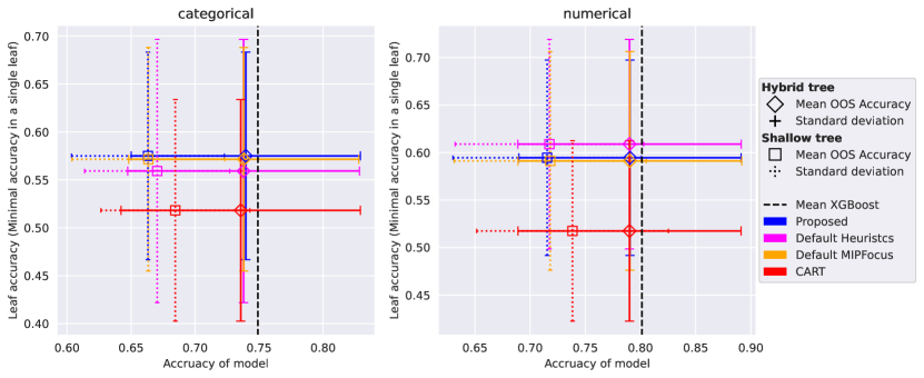
(a) Comparison of the Proposed model to models with default parameter configurations shows varying results. MIPFocus seems to influence the search only very slightly. Heuristics, on the other hand, show significant improvement on numerical datasets and a decrease in performance on categorical datasets, with about the same absolute difference.

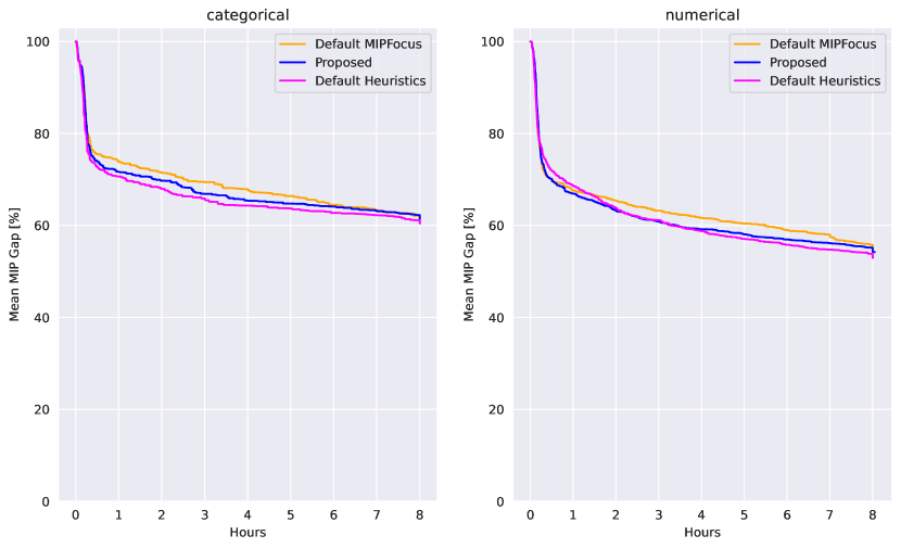
(b) Mean MIP optimality gap development over the solving time, averaged over all datasets. For a non-aggregated version, see Figure 8.

Figure 7: Comparison of models with the proposed configuration of Gurobi hyperparameters and runs with default values of the modified parameters.

The results (cf. Figure 7(a) and Tables 4, 5) show no significant improvements regarding the MIPFocus parameter. However, with the default value of the Heuristics parameter, we observe an improvement in performance on numerical datasets and a decrease in performance on categorical datasets. Both absolute differences in accuracy are about 0.015, so we opted for the variant with similar performances on both categorical and numerical datasets. That is the proposed variant focusing on heuristics. This proposed configuration also shows a more stable increase in accuracy w.r.t. the performance of CART models. The solver performance varies per dataset, as visualized in Figure 8.

These differences in performance suggest that hyperparameter space regarding the MIP solver should be further explored and could yield improvements. A closer look at Figure 8 suggests that different configurations help achieve better conditions for the solver on different datasets. This might be an area of further hyperparameter tuning based on the specific attributes of the dataset.

	Data type	Minimal	Mean ($\pm$ std)	Maximal
Leaf Accuracy	categorical	$-0.0117$	$0.0158\pm 0.0234$	$0.0531$
	numerical	$-0.1178$	$-0.0143\pm 0.0402$	$0.0435$
Hybrid-tree Accuracy	categorical	$-0.0011$	$0.0017\pm 0.0035$	$0.0094$
	numerical	$-0.0047$	$0.0005\pm 0.0025$	$0.0062$

Table 4: Detailed view of the differences in the accuracy between the default Heuristics parameter and the proposed configuration (Heuristics = 0.8). A positive number means the accuracy advantage of the proposed hyperparameter configuration. We see absolute mean differences of comparable values. The negative difference in leaf accuracy on numerical datasets also has a higher standard deviation, suggesting a stronger influence by an outlier dataset. For a graphical representation of this data, see Figure 7(a).

	Data type	Minimal	Mean ($\pm$ std)	Maximal
Leaf Accuracy	categorical	$-0.0304$	$0.0036\pm 0.0213$	$0.0299$
	numerical	$-0.0528$	$0.0034\pm 0.0342$	$0.0788$
Hybrid-tree Accuracy	categorical	$-0.0028$	$0.0016\pm 0.0043$	$0.0088$
	numerical	$-0.0026$	$0.0001\pm 0.0019$	$0.0032$

Table 5: Detailed view of the differences in the accuracy between the default MIPFocus parameter and the proposed configuration (MIPFocus = 1). A positive number means the accuracy advantage of the proposed hyperparameter configuration. Both variants seem to perform comparably, with a potential slight edge in favor of the proposed configuration. For a graphical representation of this data, see Figure 7(a).

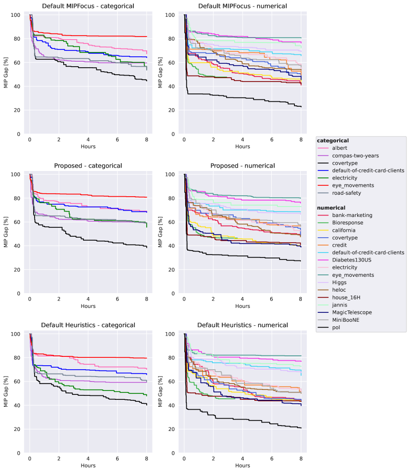
Figure 8: Mean MIP optimality gap development over the solving time averaged over 10 different train-test splits. The figure shows the progress of the value of the MIP optimality gap averaged over all splits of each dataset. Each line corresponds to one dataset. For an aggregated version, see Figure 7(b).

A.4 Memory requirements

Overall, the memory requirements of the datasets were between 15 and 95 GB. On average, all datasets required at most 70 GB of working memory. Figure 9 shows the memory requirements of our formulation in more detail. The extension phase of the process is negligible in this regard, as it requires only about 1.5 GB of working memory in total and is performed after the MIP optimization. Training and extending the CART models also required less than 2 GB of working memory.

The amount of memory required by the MIP solver is dependent on the size of the data in the number of training samples, as well as the number of features. Figure 9(b) shows this linear dependence of memory requirements on the size of the training set. Based on the coloring of the nodes, we also see the dependence on the number of features, especially in the case of the Bioresponse dataset.

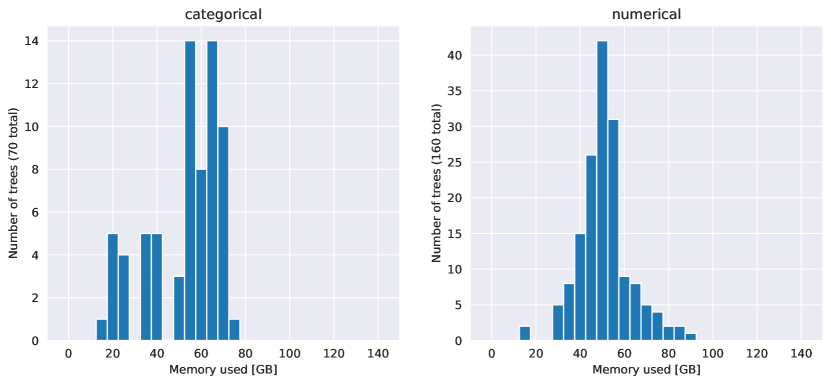
(a) Histogram of memory requirements of MIP solver for all dataset splits.

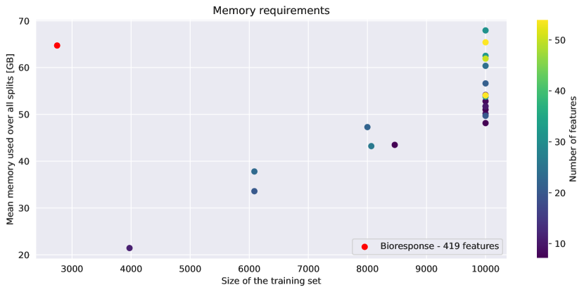
(b) Mean memory requirements on datasets. Dots are colored according to the number of features. Dataset Bioresponse is excluded from the color mapping due to having significantly more features. Training sets were truncated to a maximum of 10,000 points.

Figure 9: Memory requirements mostly do not exceed 70 GB. The memory requirements increase slightly when more time is given to the solver and significantly increase when bigger training sets are considered. We can also see some correlation between the number of features and memory requirements when looking at same-size datasets.

Performance of the model given a shorter time

When considering a shorter time for optimization, we can lower the memory requirements to levels attainable by current personal computers. When optimizing our MIP model for one hour, the required memory is below 50 GB for all datasets except Bioresponse, which has one order of magnitude more features than the rest of the datasets included in the benchmark. The mean memory requirement is below 30 GB of working memory (compared to 50 GB for the 8-hour run). See Figure 10 for details.

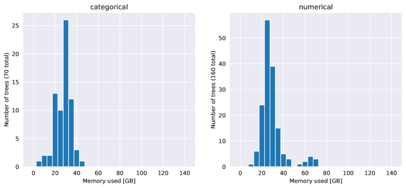
(a) Histogram of memory requirements of MIP solver for all dataset splits.

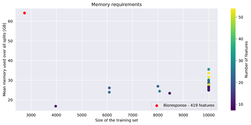
(b) Mean memory requirements on datasets. Dots are colored according to the number of features. Dataset Bioresponse is excluded from the color mapping due to having a significantly higher number of features. Training sets were clipped to a maximum of 10,000 points.

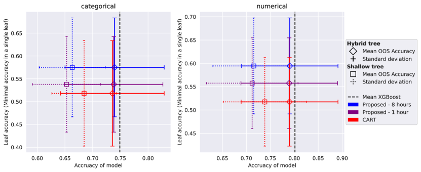
(c) Comparison of the performance of the Proposed model after 1 and 8 hours of optimization.

Figure 10: Comparison to a version of the Proposed model that the Gurobi solver optimized for only one hour. Compared to the main configuration, which ran for 8 hours, we notice a significant decrease in memory requirements for most datasets, up to tens of gigabytes. An outlier dataset Bioresponse with cca 10 times more features sees a smaller decrease of about 2 GB.

Figure 10(c) shows that even with this limited budget, we can achieve significant improvement compared to CART in leaf accuracy and similar accuracy of hybrid trees.

A.5 Reduction of the trees

The reduction phase has a beneficial influence on the leaf accuracy of a model. Figure 11 shows this improvement in mean leaf accuracy over all datasets.

In Figure 12, we further provide a comparison of the complexity of the created trees by comparing the distributions of the number of leaves (or potential explanations) provided by the method.

The maximum amount of leaves of a tree with depth 4 is 16. CART model has, on average, around 8 leaves after reduction. The proposed model’s distribution is close to the distribution of CART models. When solving the MIP formulation directly, the distribution is severely shifted toward very small trees. Our proposed method uses a default CART solution to warmstart the search, which might explain the shape of the distribution compared to the direct method and CART.

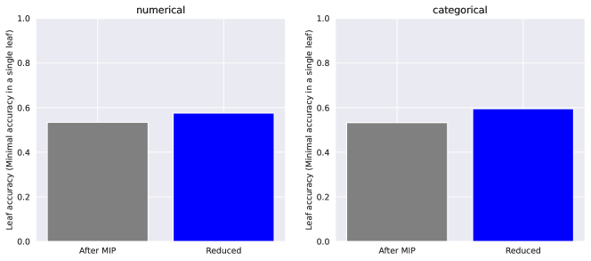
Figure 11: Effect of reduction on leaf accuracy of the model. In grey is the leaf accuracy before reduction, and in blue is the leaf accuracy after reduction. The plot shows mean accuracy over all datasets of a given type created by the proposed model.

(a) Histogram of the number of leaves of the reduced trees optimized directly using the proposed formulation. The trees are heavily pruned.

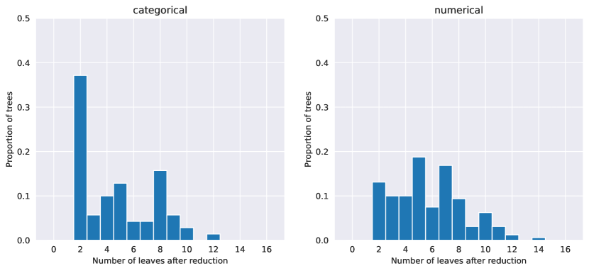
(b) Histogram of the number of leaves of the reduced trees created with the proposed formulation, warmstarted using a simple CART solution. The trees are smaller compared to well-optimized CART but retain some complexity. This was the chosen method.

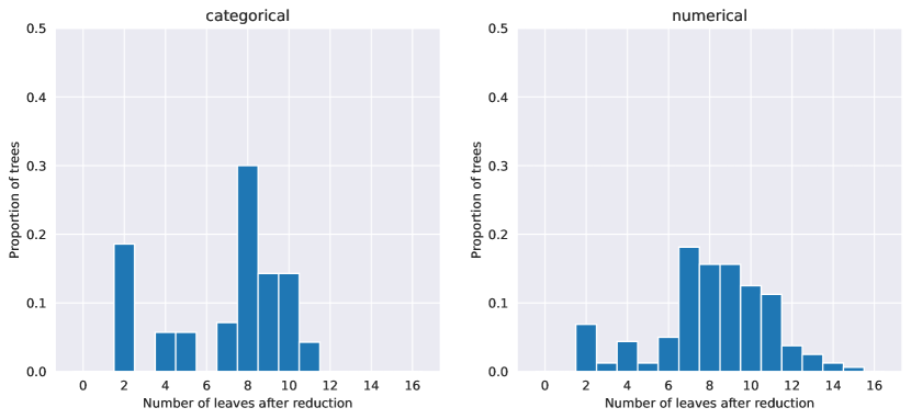
(c) Histogram of the number of leaves of the reduced trees created by CART with optimized hyperparameters.

Figure 12: Comparison of the numbers of leaves of trees after the reduction procedure.

A.6 Hyperparameter search distributions

We needed to optimize hyperparameters for extending models and CART trees used for comparisons. We used Bayesian hyperparameter search for that purpose.

Extending XGBoost models

For the hyperparameter search of XGBoost models in leaves, we used the distributions listed in Table 6. The parameters are almost all the same as those used by [Grinsztajn et al., 2022]. Only the Number of estimators and Max depth were more constrained to account for the fewer samples available for training.

The Bayesian optimization was run for 50 iterations, with 3-fold cross-validation in every leaf that contained enough points to perform the optimization. The same process was used to extend all tested trees.

Parameter name	Distribution [range (inclusive)]
Max depth	UniformInteger [1, 7]
Number of estimators	UniformInteger [10, 500]
Min child weight	LogUniformInteger [1, 1e2]
Learning rate	Uniform [1e-5, 0.7]
Subsample	Uniform [0.5, 1]
Col sample by level	Uniform [0.5, 1]
Col sample by tree	Uniform [0.5, 1]
Gamma	LogUniform [1e-8, 7]
Alpha	LogUniform [1e-8, 1e2]
Lambda	LogUniform [1, 4]

Table 6: Distributions of hyperparameters of extending XGBoost models in leaves. These were used in the Bayesian hyperparameter search in each leaf separately. All distributions except Max depth and Number of estimators are the same as in [Grinsztajn et al., 2022]. The two different distributions were selected smaller to improve the optimization time and to account for lower amounts of data.

In leaves with an insufficient amount of samples to perform the cross-validation (less than 3 samples of at least one class in our case), we train an XGBoost model with a single tree of max depth 5. In leaves with 100% training accuracy, we do not learn any model and use the majority class.

CART models

For the hyperparameter optimization of CART models, we also used Bayesian search, with the distributions shown in Table 7.

Parameter name	Distribution [range (inclusive)]
Max depth	UniformInteger [4, 4]
Min samples split	UniformInteger [2, 100]
Min samples leaf	UniformInteger [50, 50]
Max leaf nodes	UniformInteger [2, 16]
Min impurity decrease	Uniform [0, 0.2]
Cost complexity pruning parameter $\alpha$	Uniform [0, 0.3]

Table 7: Distributions of hyperparameters of CART models used to compare to our method. Max depth and Min samples in a leaf were fixed, but remain in the table for completeness.

The search was run for 100 iterations, with 5-fold cross-validation on the same training data sets as our model. After this search, the best hyperparameters were used to train the model on the full training data. The resulting tree was reduced, and every leaf was extended by an XGBoost model in the same way as our models.

A.7 Detailed results

We also provide the full results for each dataset. Figures 13 and 14 are decomposed variants of Figure 5 for categorical and numerical datasets, respectively. We also provide exact results in Tables 8 and 9, respectively. The detailed results show that the proposed model outperforms the CART model in both accuracy measures on almost all datasets and has comparable accuracy to XGBoost. Performed statistical tests (signed test and Wilcoxon’s signed-rank test) resulted in proving the statistical significance of the better performance of the proposed model, compared to CART.

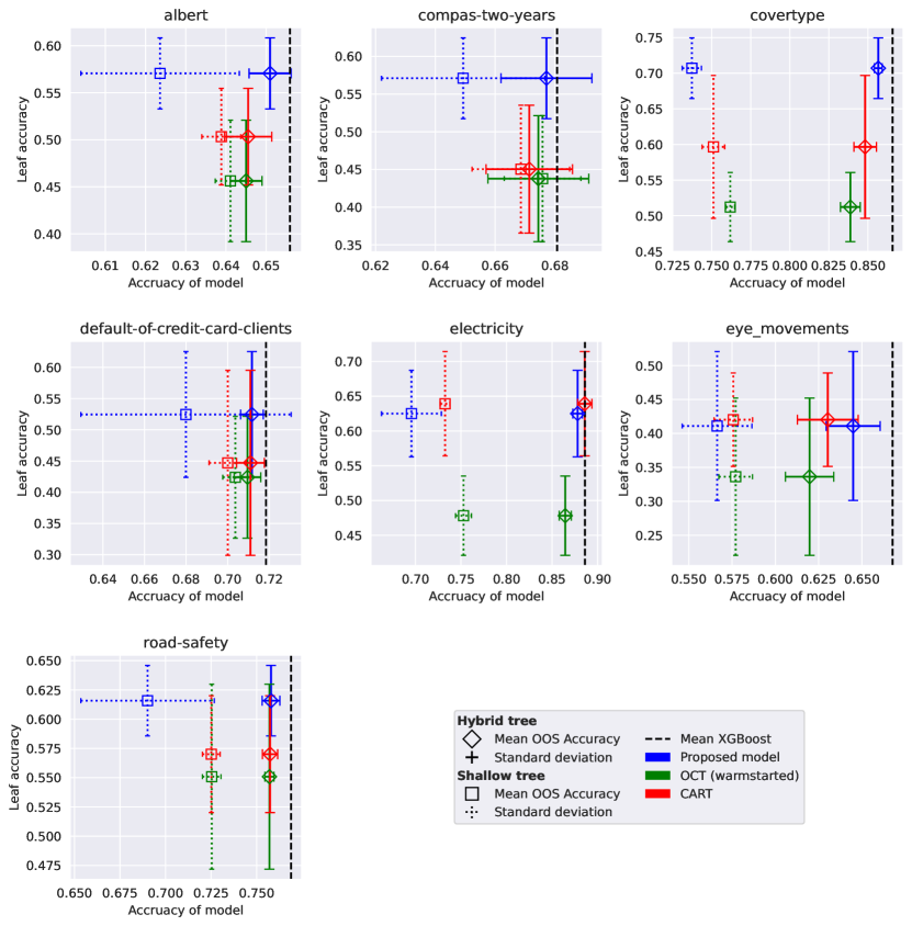
Figure 13: Detailed performance comparison of our model on categorical datasets.

	Leaf Accuracy		Hybrid-tree Accuracy
categorical datasets	CART	Proposed	CART	Proposed	XGBoost
albert	0.5033	0.5706	0.6455	0.6510	0.6559
compas-two-years	0.4504	0.5711	0.6714	0.6772	0.6807
covertype	0.5966	0.7071	0.8482	0.8567	0.8658
default-of-credit-card-clients	0.4471	0.5246	0.7110	0.7117	0.7184
electricity	0.6392	0.6250	0.8859	0.8781	0.8861
eye_movements	0.4202	0.4109	0.6303	0.6449	0.6677
road-safety	0.5701	0.6158	0.7573	0.7579	0.7689
Mean rank	1.7143	1.2857	2.8571	2.1429	1.0000

Table 8: Categorical datasets. Mean accuracy of models on out-of-sample data and average ranks.

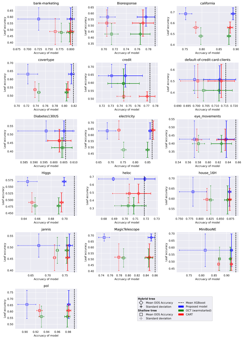
Figure 14: Detailed performance comparison of our model on numerical datasets.

	Leaf Accuracy		Hybrid-tree Accuracy
numerical datasets	CART	Proposed	CART	Proposed	XGBoost
bank-marketing	0.4861	0.5837	0.8001	0.8003	0.8044
Bioresponse	0.5201	0.5700	0.7702	0.7755	0.7920
california	0.5593	0.6861	0.8827	0.8914	0.8997
covertype	0.5365	0.6314	0.8074	0.8147	0.8190
credit	0.5153	0.6439	0.7707	0.7462	0.7738
default-of-credit-card-clients	0.5011	0.5136	0.7132	0.7124	0.7156
Diabetes130US	0.4630	0.5204	0.6028	0.6051	0.6059
electricity	0.6392	0.6331	0.8724	0.8600	0.8683
eye_movements	0.4229	0.4265	0.6343	0.6364	0.6554
Higgs	0.4910	0.5698	0.6953	0.6992	0.7142
heloc	0.4881	0.6722	0.7128	0.7188	0.7183
house_16H	0.5956	0.6336	0.8733	0.8726	0.8881
jannis	0.4550	0.5079	0.7579	0.7632	0.7778
MagicTelescope	0.5168	0.6835	0.8478	0.8518	0.8605
MiniBooNE	0.4821	0.5809	0.9192	0.9194	0.9369
pol	0.6073	0.6550	0.9810	0.9811	0.9915
Mean rank	1.9375	1.0625	2.6875	2.1875	1.1250

Table 9: Numerical datasets. Mean accuracy of models on out-of-sample data and average ranks.

A.8 Other optimization approaches

The best-performing approach of warmstarting the MIP solver with a CART solution is not the only one we tested. In Figure 15, we see a comparison of three different approaches to optimization.

• Direct refers to the straightforward use of the MIP formulation.

• Warmstarted uses a simple CART solution (created using default hyperparameters) as a starting point of the solving process.

• Gradual refers to a special process where we start by training a tree with a depth equal to 1 and use the solution found in some given time to start the search for a tree with a depth of 2, and so forth until we reach the desired depth.

All three approaches were run with the same resources. This meant that even the gradual approach took 8 hours in total. The time was distributed in a way that the available time for the optimization process doubled with each increase in depth. This means 32 minutes for the first run, 64 minutes for the tree of depth 2, 128 for depth 3, and 4 hours 16 minutes for the final tree with depth 4.

Interestingly, while the direct approach understandably does not reach a performance similar to the warmstarted variant, the gradual approach shows more promise. It has higher hybrid-tree accuracy by another 0.2 percentage points on average while having lower leaf accuracy by about 1.2 percentage points compared to the warmstarted approach (cf. Table 10).

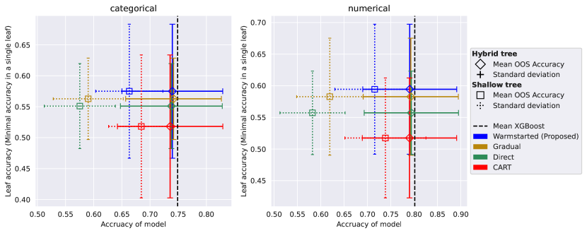
Figure 15: Comparison of the various approaches to the optimization given the same resources and conditions. Warmstarted refers to the approach of starting the optimization process with a CART solution. The gradual approach is the approach of increasing the depth of a tree and starting each new depth with the solution of the previous, shallower tree. Direct means a simple, straightforward optimization of the formulation, as it is stated, without any hints. All three approaches were run with the same resources. For a closer investigation of the Gradual approach, see Table 10.

	Data type	Minimal	Mean ($\pm$ std)	Maximal
Leaf Accuracy	categorical	$-0.1094$	$0.0122\pm 0.0753$	$0.1130$
	numerical	$-0.0867$	$0.0117\pm 0.0624$	$0.1154$
Hybrid-tree Accuracy	categorical	$-0.0219$	$-0.0021\pm 0.0094$	$0.0083$
	numerical	$-0.0103$	$-0.0023\pm 0.0056$	$0.0076$

Table 10: Comparison of Gradual and Warmstarted approach. Positive numbers show an advantage in the mean accuracy of the Proposed (Warmstarted) approach. Gradual refers to the approach when the depth of the tree is gradually increased during the optimization process.

A.9 Ablation Analyses

We provide some comparing experiments performed by changing a single hyperparameter (or a few related ones) and comparing the performance.

Unlimited depth CART

An argument could be made against our choice to compare our method to CART trees with the same limit on depth. Figure 16 and Table 11 in more detail show a comparison of CART models with a maximal depth of 4 and a maximal depth of 20. The actual depth limit for each model was optimized along with other hyperparameters using the Bayes hyperparameter optimization procedure.

Note that these tests were performed in earlier stages of testing without a fixed lower bound on the number of samples in a leaf and without cost complexity pruning. The lower bound on the number of samples was optimized using the Bayes optimization in the range [0, 50].

The aggregated results show worse performance regarding both leaf accuracy and hybrid-tree accuracy. Not only do the deeper trees perform worse, but the length of provided explanations is also well above the 5-9 threshold suggested as the limit of human understanding [Feldman, 2000].

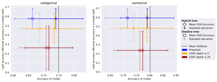
Figure 16: Comparison of CART tree results with limited depth and without such a strict limit on the depth. Deeper trees provide worse explanations (due to the length of explanation) and perform worse in both accuracy measures. For a more detailed description of the differences introduced by the depth, consult Table 11.

	Data type	Minimal	Mean ($\pm$ std)	Maximal
Leaf Accuracy	categorical	$-0.0769$	$0.2053\pm 0.2389$	$0.5404$
	numerical	$-0.1183$	$0.2441\pm 0.2115$	$0.5680$
Hybrid-tree Accuracy	categorical	$-0.0025$	$0.0173\pm 0.0185$	$0.0420$
	numerical	$-0.0006$	$0.0156\pm 0.0119$	$0.0370$

Table 11: Detailed view of the differences in the accuracy between CART trees with max depth 4 and CART trees with max depth 20. A positive number means the accuracy advantage of the more constrained model (depth $\leq 4$). For a graphical representation, see Figure 16.

Different minimum number of samples in leaves

A similar comparison is to see the performance of classically optimized lower bound on the number of samples in each leaf. Figure 17 shows a comparison of CART models when the lower bound is fixed to 50 and when it is optimized within the range from 1 to 60 using Bayesian hyperparameter optimization. The figure also includes the performance of the proposed model when $N_{\min}$ is set to 1.

It stresses the importance of setting a minimal amount of samples in leaves. Without enough points to support the leaf’s accuracy, it is more likely to be overfitted. On the other hand, when choosing the $N_{\min}$ parameter too high, we restrict some possibly beneficial splits, supported by a smaller amount of training data.

$N_{\min}$ is a critical hyperparameter, and further testing could provide more insight into the proposed model’s performance.

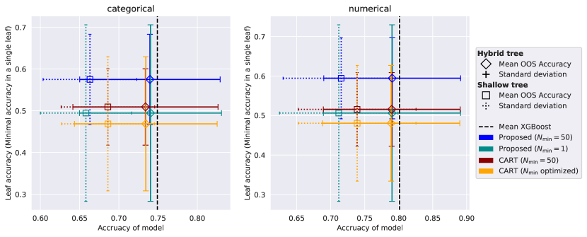
Figure 17: Comparison of performance of the proposed model with minimum samples in leaves equal 50 and 1 and of CART trees with parameter equivalent to $N_{\min}$ fixed to 50 or undergoing hyperparameter optimization. Low values of $N_{\min}$ lead to overfitting to training data and worse out-of-sample performance. Notice the high deviation of the model with $N_{\min}=1$. CART trees suffer from a similar thing, which suggests two things. Hyperparameter optimization does not opt for high $N_{\min}$ values, and this seems to be a property of trees in general, no matter how they are obtained.

Non-warmstarted OCT

We compare our method to warmstarted OCT because the proposed method also starts from the same initial CART solution. This makes them more comparable. However, we also tested the OCT variant directly optimized from the MIP formulation. See the results in Figure 18. Both OCT models were run with the same hyperparameters as the proposed model. Those being the heuristics-oriented solver, depth equal to 4, and a minimal amount of samples in leaves equal to 50.

The average OCT performs worse than all our approaches (cf. Figure 15, all approaches are above the 0.55 mark, contrary to OCT in Figure 18), but the improvement from the warmstarted variant is intriguing since it clearly manages to overtake the CART model. Especially considering that it is not caused by the direct OCT method’s inability to create complex trees without warmstarting. This is supported by Figure 19 showing a distribution of the number of leaves similar to the distribution of CART trees (cf. Figure 12). This suggests that the OCT trees have comparable tree complexity to CART and provide more valid explanations than CART, even without our extension to the formulation. This is an interesting result, considering the fact that neither CART nor OCT methods optimize for leaf accuracy.

Our model, however, more than doubles the improvement of direct OCT.

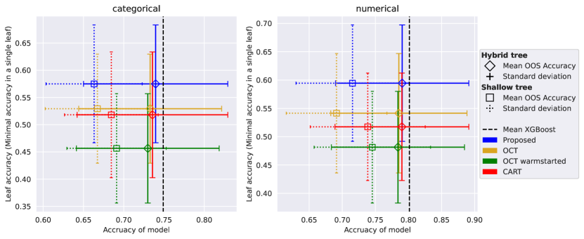
Figure 18: Comparison of OCT trees that are warmstarted the same way as our Proposed model and OCT without the warmstart, optimized directly. Interestingly, direct OCT performs significantly better.

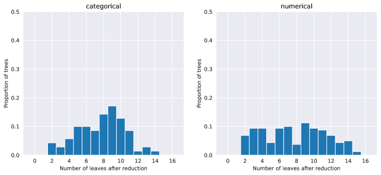
(a) Histogram of the number of leaves in the reduced trees of the direct OCT method

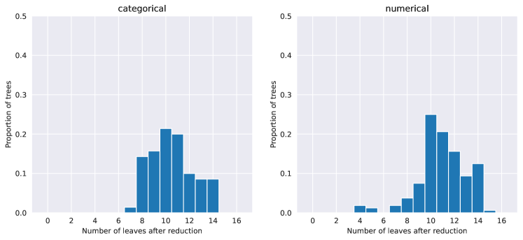
(b) Histogram of the number of leaves in the reduced trees of the warmstarted OCT method.

Figure 19: Comparison of reduced tree complexity of the OCT with and without warmstart. OCT without warmstart creates trees of similar distribution as the CART method (cf. Figure 12). And it achieves better leaf accuracy than CART (cf. Figure 18) despite neither optimizing that objective.

Deeper trees

Lastly, we provide a comparison of the proposed model of depths 4 and 5. Figure 20(a) shows better overall results for shallower trees. This is likely caused by the exponential increase in memory requirements, given the decrease in overall accuracy as well. We provide data about its memory usage in Figure 20. With a model of twice the complexity, the solver struggles to achieve comparable results to the shallower proposed model.

This is certainly a topic of further exploration by incorporating scalability improvements proposed in the literature.

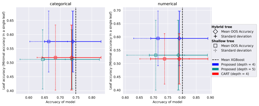
(a) Comparison of performances of the proposed model with depths 4 and 5. Shallower trees perform better, possibly because they are easier to optimize.

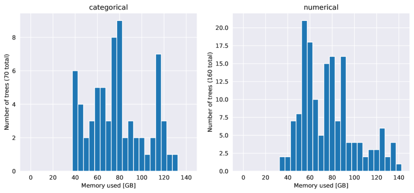
(b) Depth 5. Histogram of memory requirements of MIP solver for all dataset splits.

(c) Depth 5. Mean memory requirements on datasets. Dots are colored according to the number of features. Dataset Bioresponse is excluded from the color mapping due to having a significantly higher number of features. Training sets were clipped to a maximum of 10,000 points.

Figure 20: Comparison of the memory requirements of the Proposed model with depth 5. The mean memory requirement almost increases from cca 51.1 GB to 77.3 GB with an increase in depth from 4 to 5. Compare the above plots with Figure 9.

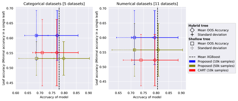
Figure 21: Comparison of a proposed model trained on at most 10,000 and 50,000 data samples. We use only datasets where the constraint caused a change, meaning we omit datasets with less than 12,500 samples. The number of datasets is in square brackets. All other presented models use only 10,000 samples, so the comparison of model accuracies is not fully representative.

A.10 More data

The 10,000 size limit on training samples was suggested by the authors of the benchmark [Grinsztajn et al., 2022]. Another good reason for such a limit is that we want our model to balance the size of the formulation and the capability of the formulated model. In other words, if we take a small amount of data, we are less likely to grasp the intricacies of the target variable distribution within the dataset. And if we take too many samples, we create a formulation that will not achieve good performance in a reasonable time.

In a comparison of a model learned on a training dataset limited to 10,000 samples with a dataset limited to 50,000 samples, we see that more data does not necessarily lead to a better model, given the same time resources, see Figure 21. The 50,000 model is worse because of the too-demanding complexity of the formulation.

It improves the model accuracy, which is unsurprising since each leaf obtains more samples. The comparison to XGBoost is unreliable since the mean value for XGBoost was computed from the performance of models trained on at most 10,000 samples.

References

- Aghaei et al. [2020] Sina Aghaei, Andres Gomez, and Phebe Vayanos. Learning optimal classification trees: Strong max-flow formulations. arXiv preprint arXiv:2002.09142, 2020.
- Arrieta et al. [2020] Alejandro Barredo Arrieta, Natalia Díaz-Rodríguez, Javier Del Ser, Adrien Bennetot, Siham Tabik, Alberto Barbado, Salvador García, Sergio Gil-López, Daniel Molina, Richard Benjamins, et al. Explainable artificial intelligence (xai): Concepts, taxonomies, opportunities and challenges toward responsible ai. Information fusion, 58:82–115, 2020.
- Athey and Imbens [2019] Susan Athey and Guido W Imbens. Machine learning methods that economists should know about. Annual Review of Economics, 11:685–725, 2019.
- Bastani et al. [2017] Osbert Bastani, Carolyn Kim, and Hamsa Bastani. Interpreting blackbox models via model extraction. arXiv preprint arXiv:1705.08504, 2017.