Zero-Shot Wireless Indoor Navigation through Physics-Informed Reinforcement Learning

Abstract

The growing focus on indoor robot navigation utilizing wireless signals has stemmed from the capability of these signals to capture high-resolution angular and temporal measurements. Prior heuristic-based methods, based on radio frequency propagation, are intuitive and generalizable across simple scenarios, yet fail to navigate in complex environments. On the other hand, end-to-end (e2e) deep reinforcement learning (RL), powered by advanced computing machinery, can explore the entire state space, delivering surprising performance when facing complex wireless environments. However, the price to pay is the astronomical amount of training samples, and the resulting policy, without fine-tuning (zero-shot), is unable to navigate efficiently in new scenarios unseen in the training phase. To equip the navigation agent with sample-efficient learning and zero-shot generalization, this work proposes a novel physics-informed RL (PIRL) where a distance-to-target-based cost (standard in e2e) is augmented with physics-informed reward shaping. The key intuition is that wireless environments vary, but physics laws persist. After learning to utilize the physics information, the agent can transfer this knowledge across different tasks and navigate in an unknown environment without fine-tuning. The proposed PIRL is evaluated using a wireless digital twin (WDT) built upon simulations of a large class of indoor environments from the AI Habitat dataset augmented with electromagnetic (EM) radiation simulation for wireless signals. It is shown that the PIRL significantly outperforms both e2e RL and heuristic-based solutions in terms of generalization and performance. Source code is available at https://github.com/Panshark/PIRL-WIN.

I Introduction

High-frequency transmissions in the millimeter wave (mmWave) bands are a key component of recently developed fifth-generation (5G) wireless systems [1, 2]. In addition to the ability to support massive data rates, the mmWave bands also enable highly accurate positioning and location capabilities [3, 4]. The wide bandwidth of mmWave signals, combined with the use of arrays with large numbers of elements, enables the resolution of paths with high temporal and angular resolution. For robotic navigation and SLAM, mmWave wireless-based positioning can be a valuable complement to camera sensors since the signals can provide information beyond line-of-sight.

This work considers a wireless indoor navigation (WIN) problem [5], where a target broadcasts periodic mmWave wireless signals and a mobile robot (agent) has to locate and navigate to the target. Importantly, the environment is initially unknown to the agent. While there has been considerable research on such navigation problems from camera data (see, for example, a survey of deep reinforcement learning methods in [6]), the question is how to leverage the mmWave wireless signals. A growing body of research attempts to address this question [7, 8, 5], where heuristic solutions are developed based on the physics properties of mmWave. For example, [5] presents a simple heuristic navigation strategy based largely on following the angle of arrival (AoA) of wireless signals. This physics-based solution has the advantage that it requires no training and thus does not overfit any specific environment, displaying decent zero-shot generalization. However, this heuristic fails to handle complex wireless environments where mmWave signals propagate along multiple paths through reflections and diffractions [9]. Moreover, observations of these paths are inexact due to noised measurements.

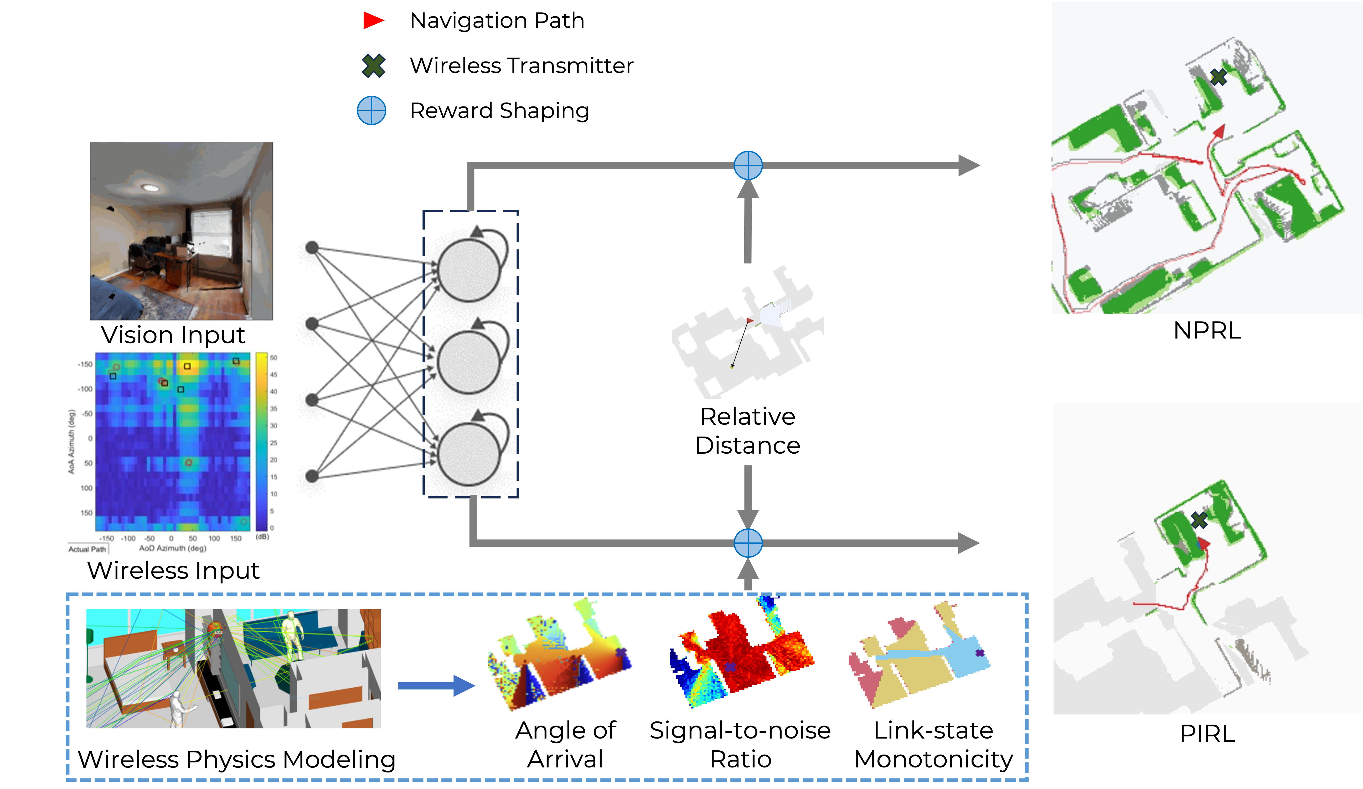
Figure 1: The wireless indoor navigation (WIN) requires the agent to navigate to the wireless transmitter in an unknown environment using multi-modal input, including vision and wireless. The non-physics e2e RL (NPRL), based on relative distance cost, fails to navigate efficiently in unseen scenarios. Trained to utilize physics prior, physics-informed RL (PIRL) acquires zero-shot generalization with interpretable policies.

When facing such complex indoor navigation tasks, deep reinforcement learning (RL) offers an end-to-end (e2e) learning framework without manual design. Powered by deep representation learning, e2e RL can learn rich policies from complex heterogeneous sensor data. However, such a practice requires hundreds of GPU hours and an exorbitant volume of training data [10]. The resulting policy tends to overfit the training environment, generalizing poorly [11] or requiring pre-exploration when tested in a new environment [8].

To combine the best of two worlds, this work proposes a physics informed RL (PIRL) approach, training the agent to utilize physics information through reward shaping. As illustrated in Figure 1, the key idea is to use e2e RL but with a relative-distance-based cost function augmented with physically-motivated terms, encouraging the policy to seek actions conforming to physical principles that lead to shorter paths. For the WIN problem, the physical terms include attempts to increase the signal strength, follow the angle of arrival, and navigate to regions where the number of reflections for the strongest path is reduced. Since these physics principles hold across different wireless environments, the proposed PIRL alleviates catastrophic forgetting: previously acquired knowledge is carried over to the ensuing training tasks, leading to sample-efficient learning. Additionally, trained to leverage physics information, the PIRL agent can deal with unseen environments without fine-tuning, achieving zero-shot generalization.

We corroborate the proposed PIRL method using a widely-used AI Habitat indoor navigation dataset [10] combined with detailed RF propagation simulation developed in [5]. This synthesized simulator is referred to as the indoor wireless digital twin (WDT). Our contributions are as below.

1. We propose a physically-motivated reward shaping to achieve physics-informed RL for WIN, enjoying a simple implementation, see (2).

2. We demonstrate that the PIRL requires fewer training samples/resources than vanilla e2e RL does (1593 v.s. 2304 GPU-hours), which is particularly valuable in the WIN problem where wireless simulation is expensive;

3. Our testing experiments show that PIRL generalizes significantly better to new environments in a zero-shot manner, compared with heuristic/RL-based baselines;

4. Inspired by recent advances in explainable AI [12], we conduct sensitivity analysis on the learned PIRL model regarding the input wireless data, showing that the PIRL’s actions are interpretable in that they are consistent with physics principles embedded in the reward shaping.

II Related Work

Our work subscribes to the recent line of research on indoor positioning and localization using high-frequency wireless bands [3, 4, 8, 5]. Closely related to this work, [5] considers the same WIN setup and proposes a physics-based heuristic: following the AoA, which proves effective in simple scenarios but inadequate when facing complex wireless environments. Similar to our PIRL, [8] develops a deep-learning-based localization algorithm, yet it requires additional map generation for indoor navigation. In contrast, our PIRL incorporates physics knowledge into the RL model, delivering efficient navigation in unexplored environments.

This work also falls within the burgeoning field of physics-informed machine learning, which amounts to introducing appropriate observational, inductive, and learning biases that facilitate the learning process [13]. Our proposed PIRL adopts the last approach: incorporating learning biases, i.e., the physics-motivated reward shaping. By selecting appropriate loss functions to modulate the training, the PIRL favors convergence to solutions adhering to underlying physics. Similar methodologies have been applied to nuclear assembly design [14], aircraft conflict resolution [15], and ramp metering [16]. To the best of our knowledge, this work is among the first endeavors to investigate the physics principles in the 5G wireless domain for RL-based indoor navigation. We refer the reader to Appendix A for an extended discussion.

III Wireless Indoor Navigation: Task Setup

Consider the WIN task setup in [5], where a stationary target is positioned at an unknown location in an indoor environment. The target is equipped with a mmWave transmitter that broadcasts wireless signals at regular intervals. Equipped with a mmWave receiver, an RGB camera, and motion sensors, the agent aims to navigate to the target in minimal time. In contrast to the PointGoal task [17], WIN does not provide the agent with the target coordinates. The detailed environment setup and the agent’s actuation/sensor models are provided below.

The agent pose is represented by $p=(x,y,\varphi)$ where $x,y$ denotes the $xy$-coordinate of the agent measured in meters, and $\varphi$ represents the orientation of the agent in radius (measured counter-clockwise from $x$-axis). Without loss of generality, we assume that the agent starts at $p_{1}=(0,0,0)$. The agent aims to locate and navigate to the target (the wireless transmitter) denoted by $(x^{*},y^{*})$. We consider a WIN task where the agent operates in the presence of multiple kinds of information feedback that we denote with a vector $o_{t}=(m_{t},\hat{p}_{t},v_{t},w_{t})$, where $t$ is the time step, $m_{t}$ is an estimate map, $\hat{p}_{t}=(x_{t},y_{t})$ is the estimated pose, $v_{t}=V(p_{t})$ represents visual information and $w_{t}=W(p_{t})$ represents the wireless information.

Map and Pose

The map and pose estimates can come from any SLAM module. In the simulations below, we will use the state-of-the-art neural SLAM module proposed in [18] that provides robustness to the sensor noise during navigation. This SLAM module internally maintains a spatial map $m_{t}$ and the agent’s pose estimate $\hat{p}_{t}$ (different from the raw sensor reading $\bar{p}_{t}$) at each time step during the navigation process. The spatial map is represented as $m_{t}\in[0,1]^{2\times M\times M}$ is a 2-channel $M\times M$ matrix, where $M\times M$ denotes the map size and each entry corresponds to a cell. Let $d$ denote the width of the map discretization so each cell is $d\times d$, and the total area is $Md\times Md$, $d=$ $25\text{\,}\mathrm{c}\mathrm{m}$. Entries of the first channel of $m_{t}$ denote the probabilities of obstacles within the corresponding cells, while those of the second channel represent the probabilities of the cells being explored [18].

Wireless Information

$W(p)=(g_{n},\Omega_{n}^{rx},\Omega_{n}^{tx})_{n=1}^{N}\in\mathbb{R}^{3\times N}$, where $N$ is the maximum number of detected paths along which signals propagate. For the $n$-th path, $g_{n}$ denotes its signal-to-noise ratio (SNR), $\Omega_{n}^{rx}$ and $\Omega_{n}^{tx}$ denote the angle of arrival (AoA) and departure (AoD), respectively. We consider the top $N=5$ paths with the strongest signal strengths among all paths(see [5] and Appendix F).

Visual Information

$V(p)\in\mathbb{R}^{3\times L_{1}\times L_{2}}$ is the 3-channel RGB camera image input at the pose $p$, where $L_{1}$ and $L_{2}$ denote the height and the width, respectively. In addition to the wireless sensor and the camera, the agent is also equipped with motion sensors. The sensor readings lead to the estimate of the agent pose $\bar{p}=(\bar{x},\bar{y},\bar{\varphi})$, which can be different from the agent’s authentic pose $p$. The difference $\varepsilon_{sen}=\bar{p}-p$ is referred to as the sensor noise.

Actuation

Following [18], we assume the agent utilizes three default navigation actions, $\mathcal{A}:=\{a_{F},a_{L},a_{R}\}$. Here, $a_{F}=(d,0,0)$ denotes the moving-forward command with a travel distance equal to the grid size $d=$ $25\text{\,}\mathrm{c}\mathrm{m}$; and $a_{L}=(0,0,-10^{\circ})$ and $a_{R}=(0,0,10^{\circ})$ stand for the control commands: turning left and right by 10 degrees, respectively.

IV Physics-Informed Reinforcement Learning

Navigating within an unknown environment can be viewed as sequential decision-making using partial observations. The agent’s state is given by its authentic pose $p_{t}$ that remains hidden, and only partial information $o_{t}$ collected by sensors is available for decision-making at each time step. The state transition as shown in the actuation model presented in Section III is Markovian: $p_{t+1}=p_{t}+a_{t}$. Hence, the WIN task is a partially observable Markov decision process (POMDP), with the observation kernel too complicated to be analytically modeled.

The navigation performance can be measured through a cost function defined as the Euclidean distance (or any distance metric, e.g., geodesic distance) between the current pose and the target position $c_{t}=\|x_{t}-x^{*}\|^{2}+\|y_{t}-y^{*}\|^{2}$. Denote by $\mathcal{H}_{t}:=\{(o_{k},a_{k})_{k=1}^{t-1},o_{t}\}$ the set of all possible observations up to time $t$, and by $\mathcal{H}:=\cup_{t=1}^{H}\mathcal{H}_{t}$ the union of all histories, where $H$ denotes the horizon length. The agent’s objective in WIN is to find an optimal policy $\pi:\mathcal{H}\rightarrow\mathcal{A}$ such that the cumulative cost $\mathbb{E}_{\pi}[\sum_{t=1}^{H}c_{t}]$ is minimized, implying that the agent navigates to the target in minimal time.

Deep RL

The planning algorithms for POMDP [19] are not suitable for WIN, since the state and the observation space are of high dimensions and continuum, and the observation kernel remains unknown. To create model-free learning-based navigation, one can apply deep reinforcement learning, such as proximal policy optimization (PPO) [20], to approximately solve the cost-minimization problem in (1), where the policy $\pi$ is represented by an actor-critic neural network [21], and its model weights are denoted by $\theta\in\mathbb{R}^{d}$.

$$\min_{\theta}\mathcal{L}_{\rm RL}(\theta):=\mathbb{E}_{\pi(\theta)}C_{\rm RL},\quad C_{\rm RL}=\sum_{t=1}^{H}c_{t},$$ (1)

To address the partial observability in WIN, we incorporate a recurrent module [22] into the actor-critic network architecture. With the recurrent neural network (RNN), the policy $\pi(\theta)$ need not take in all past observations $\{(o_{k},a_{k})_{k=1}^{t-1},o_{t}\}$, and instead, the current partial observation suffices, as RNN can memorize historical input and integrate information feedback across time [22]. For more details on the RL implementation, including PPO and RNN, we refer the reader to Appendix C. We refer to RL with the loss function (1) as non-physics-based RL (NPRL), to differentiate it from the physics-informed RL to be described shortly.

Insufficiency of End-to-End DRL

We observe in the experiments that when NPRL policies are applied to the WIN problem, they exhibit poor generalization ability and sample efficiency. For example, the NPRL agent trained for one task (a given map and one target position within the map) even fails to navigate to another target within the same map. Due to multiple reflections and diffractions of mmWave, the wireless field $W(p)$ changes drastically when the transmitter moves from one location to another, especially when the indoor environment displays complex geometry. Consequently, model weights learned for (overfit) one task are barely relevant to another. In addition to limited generalization, the NPRL agent requires an astronomical amount of samples due to catastrophic forgetting. Since wireless fields vary across different tasks, knowledge of the previously learned task may be abruptly lost as information relevant to the current task is incorporated. Hence, the NPRL agent needs to be re-trained under previous tasks, leading to time-consuming shuffle training [10].

Physics-Informed Reinforcement Learning (PIRL)

Physics-informed RL (PIRL) or machine learning has emerged as a promising approach to simulate and tackle multiphysics problems in a sample-efficient manner [13]. The gist is that neural networks can be trained from additional information obtained by enforcing physics laws. Existing general-purpose strategies of distilling the physics-domain-knowledge into the RL agent include supervised-learning approaches such as imitation learning [23], and RL approaches such as offline/batch RL [24, 25] and vanilla RL, i.e., online policy learning, where the agent repeatedly interact with the digital twin to acquire feedback. This work considers the simple online learning approach because we need a fair comparison between our proposed PIRL and other baseline wireless navigation approaches that are based on online RL on sample efficiency and generalization.

Adopting online RL, we thus propose to simply augment the cost with physically-motivated reward shaping. Specifically, the augmented cost function is as below.

$$\mathcal{L}(\theta):=\mathbb{E}_{\pi(\theta)}\left[C_{\rm RL}+\lambda_{\rm LS}C_{\rm LS}+\lambda_{\rm AoA}C_{\rm AoA}+\lambda_{\rm SNR}C_{\rm SNR}\right],$$ (2)

where the additional terms are motivated by physics principles in WIN: $C_{\rm LS}$, for link-state monotonicity, $C_{\rm AoA}$ for angle of arrival direction following, and $C_{\rm SNR}$ for SNR increasing. $\lambda_{\rm LS}$, $\lambda_{\rm AoA}$, and $\lambda_{\rm SNR}$ are weighting constants. The following presents the three physics-informed terms.

Monotonicity of Link States

In mmWave applications, link states are of great importance [5, 1], which are primarily categorized into Line-of-Sight (LOS) and Non-Line-of-Sight (NLOS). A location $(x,y)$ (or equivalently a pose $p$) is said to be of LOS if there is a wireless signal path wherein electromagnetic waves traverse from the source to the receiver without encountering any hindrances. In contrast, NLOS signifies the absence of such a direct visual path. NLOS can further be subdivided into first-order, second-order, third-order, and so forth. First-order NLOS (1-NLOS) implies that at least one electromagnetic wave in the wireless link undergoes a single reflection or diffraction. Likewise, second-order NLOS (2-NLOS) suggests at least one electromagnetic wave undergoing two instances of reflection or diffraction. Similar arguments apply to higher-order NLOS, denoted by $2^{+}$-NLOS. Define $\ell(p)\in\{0,1,2\}$ as the link state of the pose $p$, where the link state evaluation $0$, $1$, and $2$ represent the LOS (0-NLOS), 1-NLOS, and $2^{+}$-NLOS scenarios, respectively. Note that the link state is a wireless terminology instead of the actual state input to be fed into RL models. Instead, the agent learns to infer the link state from the raw wireless input $W(p)$ [5].

Figure 2(a) presents a distribution map of link state for indoor wireless signals. The purple cross represents the target location. The LOS coverage, by definition, is a connected area, unlike $1$-NLOS, and $2^{+}$-NLOS coverage. Hence, when the agent enters the LOS area, the shortest path to the target is the straight line connecting the two (see Figure 2(a)), which remains within the LOS area. Another important observation is that the LOS area must be bordered by $1$-NLOS, which is then bordered by $2$-NLOS, and so forth. In other words, if the link state increases as the agent navigates, the resulting path cannot be optimal. This observation leads to the statement that a necessary condition for a path to be optimal is that the link state decreases monotonically along the path, which motivates the term $C_{\rm LS}=\sum_{t}\max\{0,{\ell}_{t}-{\ell}_{t-1}\}$. The proof is included in Appendix B.

Reversibility of mmWaves

Similar to the principle of reversibility of light, the mmWave follows the same path if the direction of travel is reversed. This reversibility principle leads to a simple yet effective navigation strategy: following the angle of arrival (AoA) of the strongest path, which experiences the least number of reflections. Besides, [5] shows that following the AoA of the strongest path in 1-NLOS cases (NLOS with a single reflection) generally leads to decent navigation since it tends to find a route around the obstacle. However, for 2-NLOS cases (${\ell}_{t}=2$), following the AoA may not be a reliable solution, since it arises from multiple reflections or diffractions. To impose this angle tracking, we add the term $C_{\rm AoA}=\sum_{t=1}^{H}|\hat{\Omega}_{t}-\Omega^{rx}_{1,t}|^{2}\cdot\mathds{1}_{\{{\ell}_{t}\neq 2\}}$ into (2) where $\hat{\Omega}_{t}$ is the agent’s moving direction derived from the action and $\Omega^{rx}_{1,t}$ is the AoA of the strongest path included in the wireless information $w_{t}$.

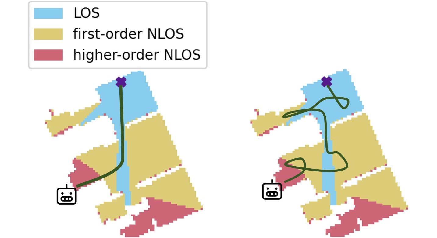
(a) The link state decreases monotonically along the shortest path.

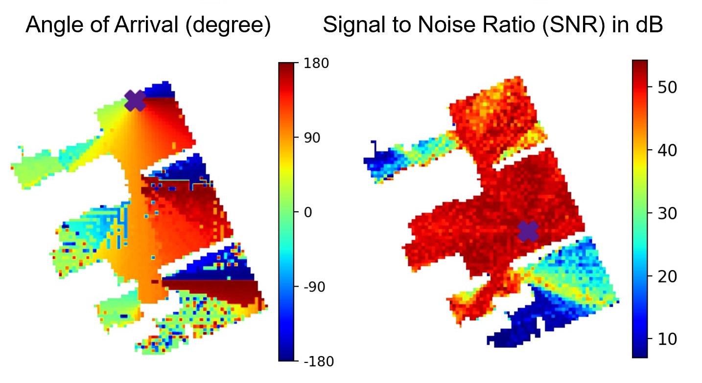
(b) The agent can move reversely along the AoA and explore high SNR area in NLOS.

Figure 2: The physics principles in WIN.

Navigation in $2^{+}$-NLOS and the Gradient Field of SNR

Due to reflections, diffractions, and measurement noises, the reversibility principle is less effective in $2^{+}$-NLOS. Denote by $g(p)=\sum_{i}g_{i}(p)$ the overall SNR at the pose $p$, or equivalently, the location $(x,y)$. A key observation is that $g$ displays remarkable declines in the transit from the LOS and 1-NLOS to $2^{+}$-NLOS areas, see Figure 2(b). Upon statistically analyzing 21 maps, it is observed that navigating from the 1-NLOS position to the nearest $2^{+}$-NLOS position leads to an average decline of $25.2\text{\,}\mathrm{d}\mathrm{B}$ in SNR. Hence, we propose a navigation heuristic in $2^{+}$-NLOS scenarios: the agent should move along the reverse direction of the SNR gradient field $-(\nabla_{x}g,\nabla_{y}g)$ (finite differences in practice), i.e., toward the direction with the stronger signal strength. We remark that such a heuristic is less helpful in the LOS and 1-NLOS, where $\nabla g$ is relatively insubstantial: the difference between SNRs of two adjacent mesh vertices is mostly within $3\text{\,}\mathrm{d}\mathrm{B}$. To encourage the policy to increase in SNR, we add the cost $C_{\rm SNR}=\sum_{t=1}^{H}|\hat{\Omega}_{t}-\nu_{t}|^{2}$ where $\nu_{t}$ denotes the angle between $-\nabla_{x,y}g(p_{t})$ and the $x$-axis. In numerical implementations, $\nu_{t}$ is replaced by the steepest descent direction approximated using finite differences of the mesh points (see Appendix C).

What does PIRL learn?

One important observation is that the physics-based reward shaping is not a potential-based transformation [26]. To see this, consider a sequence of poses $p_{1}\rightarrow p_{2}\rightarrow\cdots\rightarrow p_{n}\rightarrow\cdots\rightarrow p_{1}$ such that the agent can travel through them in a cycle, which can incur a net positive cost, e.g., $C_{\rm LS}$ is strictly positive when traversing from LOS to NLOS and then back to LOS. Hence, the policy invariance theorem [26] tells that (2) leads to a navigation policy distinct from the shortest path prescribed by (1). For example, following AoA in the 1-NLOS may yield a detour around a corner rather than the shortest path. Even though PIRL is not optimal, it targets suboptimal solution $\theta_{PIRL}$ shared across various tasks (because physics principles are invariant) as shown in Figure 3. The shared suboptimality alleviates catastrophic forgetting in training and creates zero-shot generalization in testing.

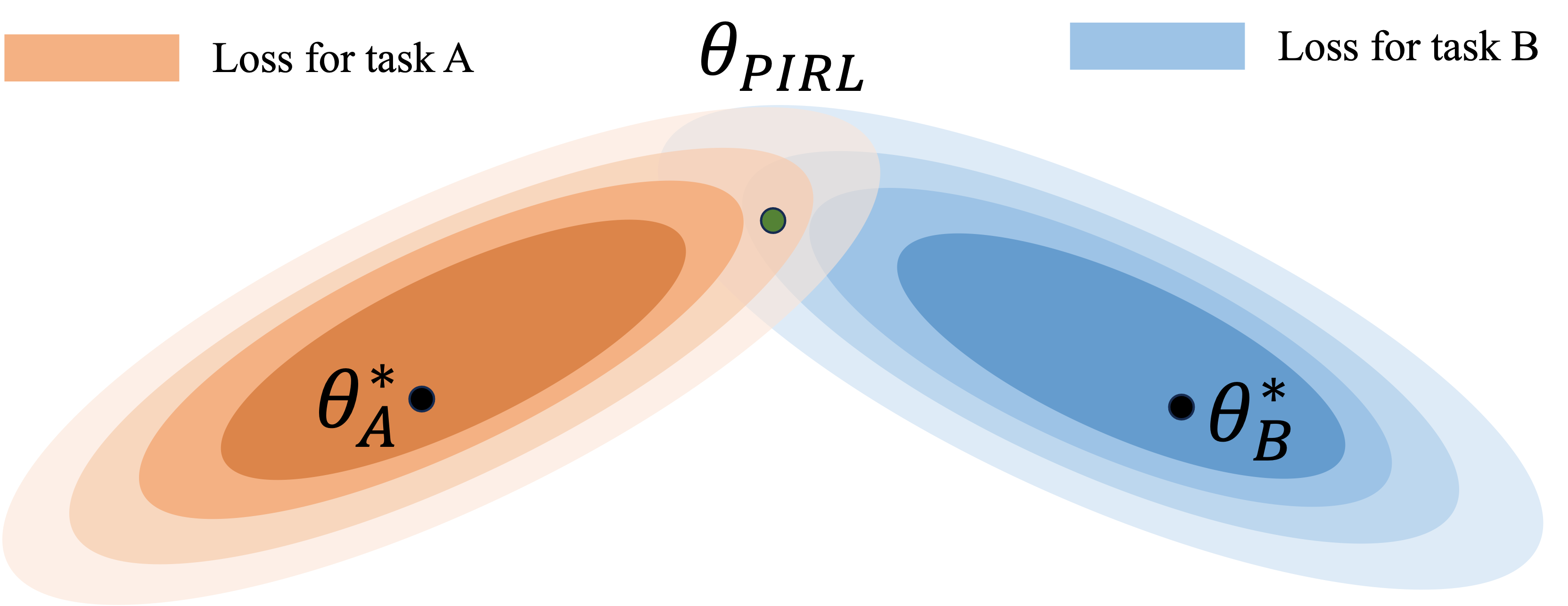
Figure 3: PIRL targets the suboptimal $\theta_{PIRL}$ shared by various tasks, instead of optimal policies $\theta_{A}^{*}$, $\theta_{B}^{*}$ for individual tasks.

V Experiments

This section evaluates the proposed PIRL approach for WIN tasks, aiming to answer the following questions. 1) Sample Efficiency: does the PIRL take fewer training data than the non-physics-based baseline? 2) Zero-shot Generalization: can PIRL navigate in unseen wireless environments without fine-tuning? 2) Interpretablility: does the PIRL conform to the physics principles, leading to interpretable navigation? We briefly touch upon the training procedure, and the experiment setup in the ensuing paragraph, and details are deferred to Appendix D. The experiment includes 21 different indoor maps (15 for training; 6 for testing) from the Gibson dataset labeled using the first 21 characters in the Latin alphabet ($A,B,\ldots,U$), and each map includes ten different target positions labeled using numbers ($1,2,\ldots,10$). The agent’s starting position is fixed for each map regardless of the target position, depending on which, the ten targets for each map are classified into three categories. The first three targets ($1-3$) are of LOS (i.e., the agent’s starting position is within the LOS area), the next three ($4-6$) belong to $1$-NLOS, and the rest four ($7-10$) correspond to $2^{+}$-NLOS scenarios. For each task (e.g., A1), the maximum number of training episodes is 1000, and the training process terminates if the agent completes the task in more than 6 episodes out of 10 consecutive ones.

We consider three baseline navigation algorithms. 1) non-physics-based RL (NPRL): the RL policy is of the same architecture as our proposed PIRL, whereas the reward function is not physics-informed, i.e., only $\mathcal{L}_{RL}$ in (1). 2) Wireless-assisted navigation (WAN): this non-RL-based method, put forth in [5], relies on a physics-based heuristic that utilizes wireless signals (following AoAs) exclusively within LOS and 1-NLOS scenarios while exploring randomly in $2^{+}$-NLOS. WAN uses a pre-trained classification model to infer the link state. The above two are primarily baselines since our PIRL is a hybrid of the two methodologies. Additionally, to highlight the necessity of leveraging wireless signals in indoor navigation, we consider the third baseline: Vision-augmented SLAM (V-SLAM), which is a vison-augmented version of the active neural SLAM (AN-SLAM) in [18]. V-SLAM only takes in RGB image data without wireless inputs. The V-SLAM agent is capable of localizing the target once it falls within the visual (LOS), whereas in the NLOS, V-SLAM reduces to the AN-SLAM, aiming to explore as much space as possible. Our experiments use the pre-trained vision model and neural-SLAM module.

Sample Efficiency

We first evaluate the sample efficiency of the PIRL training process by comparing the number of training episodes of PIRL in LOS, 1-NLOS, and $2^{+}$-NLOS with those of NPRL. The bar plot in Figure 4 gives a visualization of the sample efficiency in the training phase on map A (the first map used in the training) and I (midway in the training). In the early stage of the training, no remarkable difference between the two is observed. Yet, as the training proceeds, PIRL demonstrates a superior sample efficiency on map I, compared with NPRL. This is because the PIRL agent learns to utilize the physics principles that persist across different wireless fields, after being trained on first a few maps. One can see that the PIRL policy already acquires generalization ability to some extent at this point, such that lightweight training would be sufficient for navigating in new environments. In contrast, the NPRL agent, using vanilla end-to-end learning, may be confused when exposed to drastically different wireless fields. Hence, the prior experience does not carry over to the new environment, and NPRL needs to learn almost from scratch.

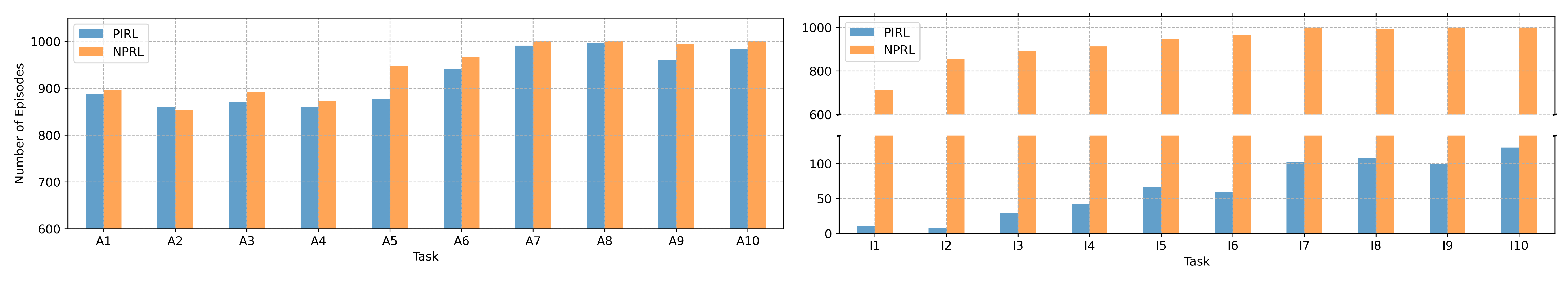
Figure 4: The number of episodes for ten tasks in map A and I. For each map, task number 1-3, 4-6, and 7-10 are tasks of LOS, $1$-NLOS, and $2^{+}$-NLOS case, respectively. Compared with NPRL, PIRL requires fewer and fewer episodes on each case as the training progresses.

Generalization

We first highlight that our testing environments (new maps with different target positions) are structurally different from training cases. Different room topologies and wireless source locations create drastically different wireless fields unseen in the training phase, as the reflection and diffraction patterns are distinct across each setup. We collect the testing performance of three baselines and our PIRL on maps $P$ to $U$, and report the average results of 20 repeat tests under different random seeds. Since baselines and PIRL use different reward designs, we consider the metric normalized path length (NPL) defined as the ratio of the actual path length (the number of navigation actions) over the shortest path length of the testing task (the minimal number of actions). The closer NPL is to 1, the more efficient the navigation is. The comprehensive comparison is summarized in Table IV in Appendix E, and Figure 5 gives a visualization of NPLs averaged over the LOS task (e.g. $P1-3$), the 1-NLOS (e.g., $P4-6$), and the $2^{+}$-NLOS (e.g., $P7-10$) on testing maps $P$ and $T$. Our PIRL policy generalizes well to these unseen tasks and achieves the smallest NPLs across all three scenarios. In addition to NPL, we also report in Figure 5 the Success weighted by (normalized inverse) Path Length (SPL) and in Table I the success rate, which are customary in the literature [17].

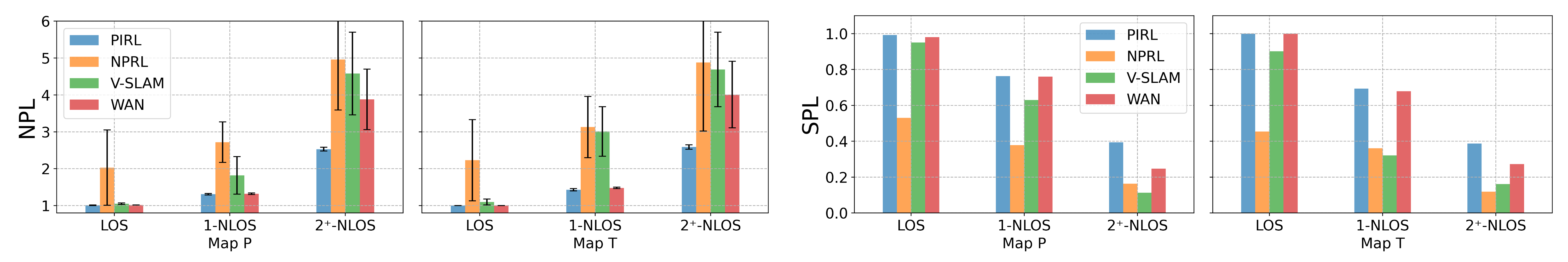
Figure 5: Average NPLs (left) and SPLs (right) returned by navigation policies in the testing. Unlike NPL, SPL uses the inverse of the path length, and hence, the smaller the SPL one returns, the better it is. Since SPL assign zeros to unsuccessful navigation instances, we do not report its error bar.

TABLE I: Success Rates in Map T and Map P.

		PIRL	NPRL	V-SLAM	WAN
Map T	LOS	1	1	1	1
	1 NLOS	1	1	1	1
	2+NLOS	1	0.4	0.65	0.9
Map P	LOS	1	1	1	1
	1 NLOS	1	1	1	1
	2+NLOS	1	0.45	0.4	0.85

Interpretable Navigation

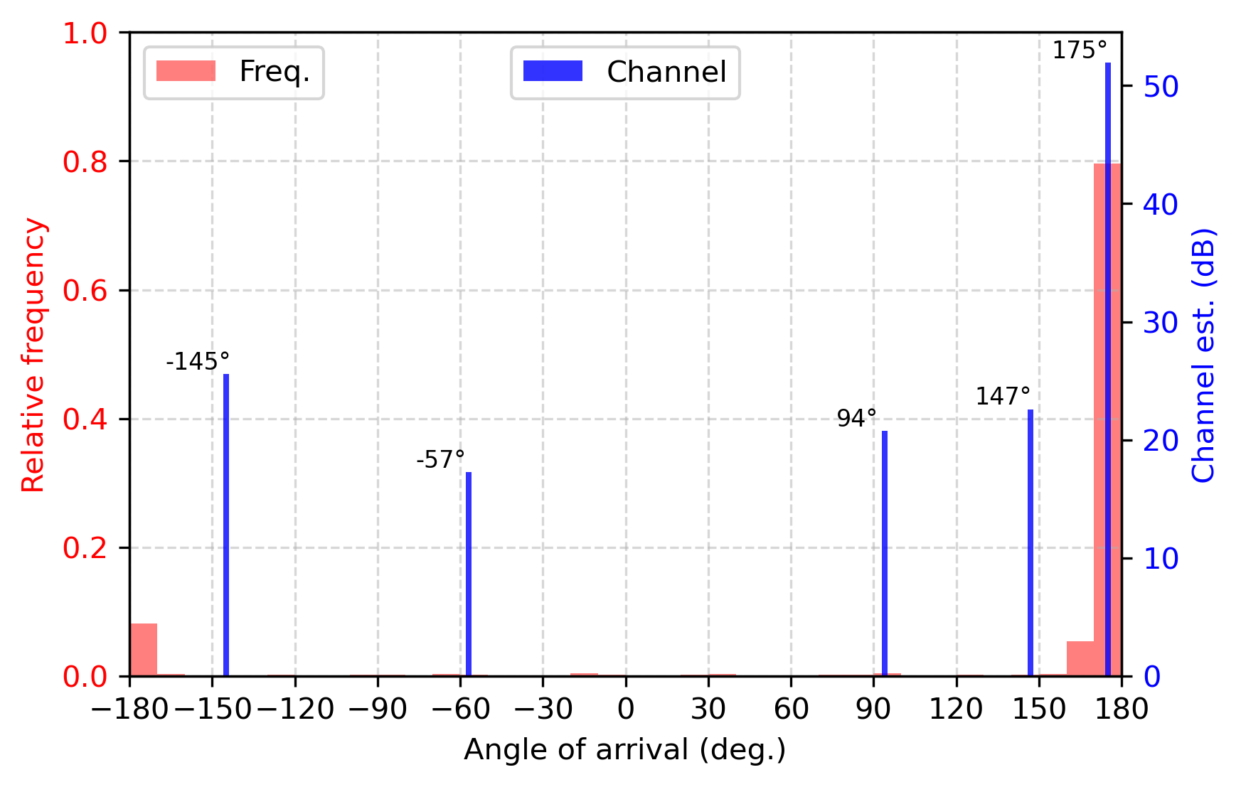
(a) In the LOS, PIRL follows the AoA of the first channel (strongest path).

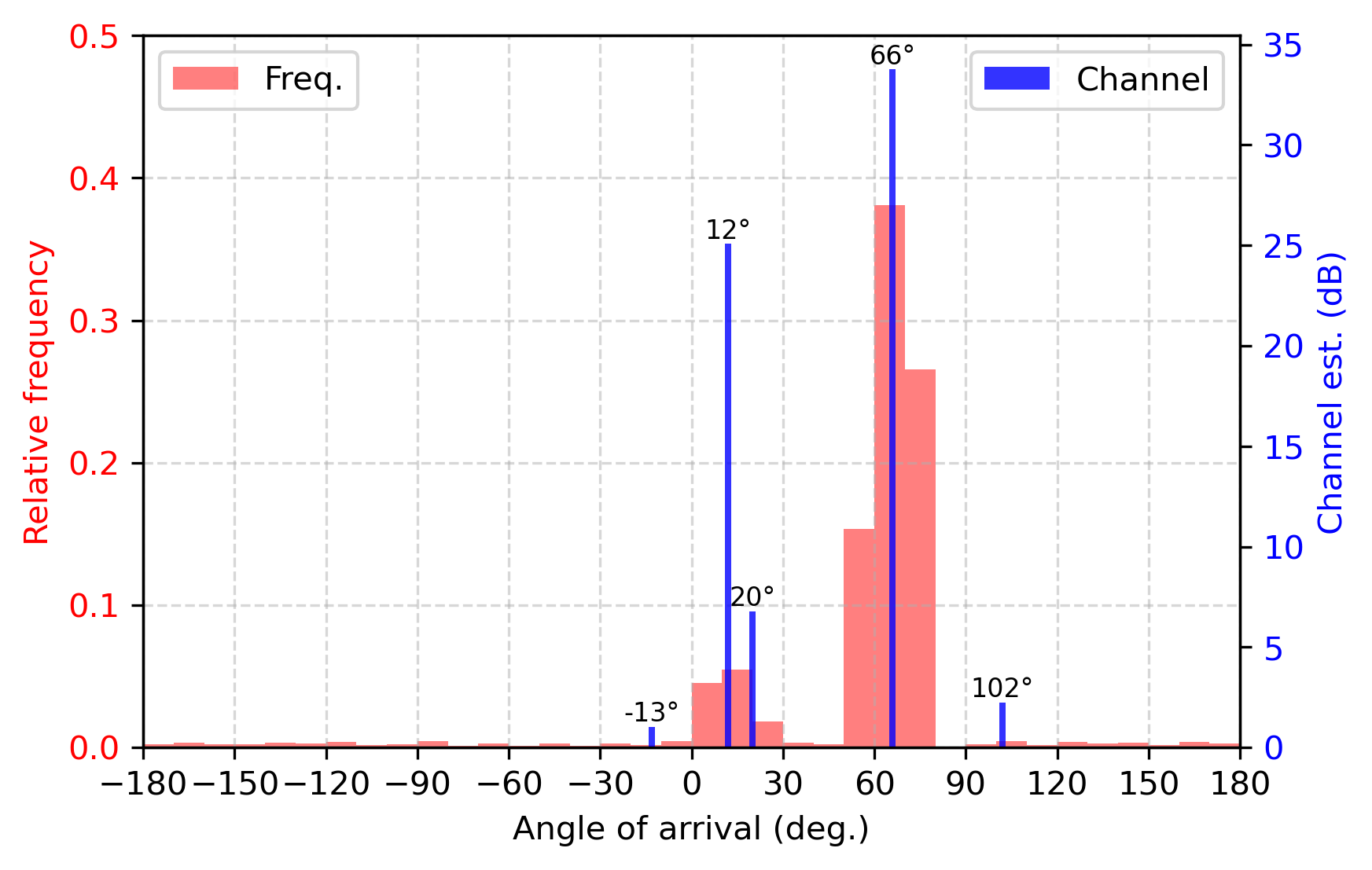
(b) In the 1-NLOS, PIRL follows the AoA of the strongest channel.

(c) In the $2^{+}$-NLOS, PIRL aims at high-SNR directions.

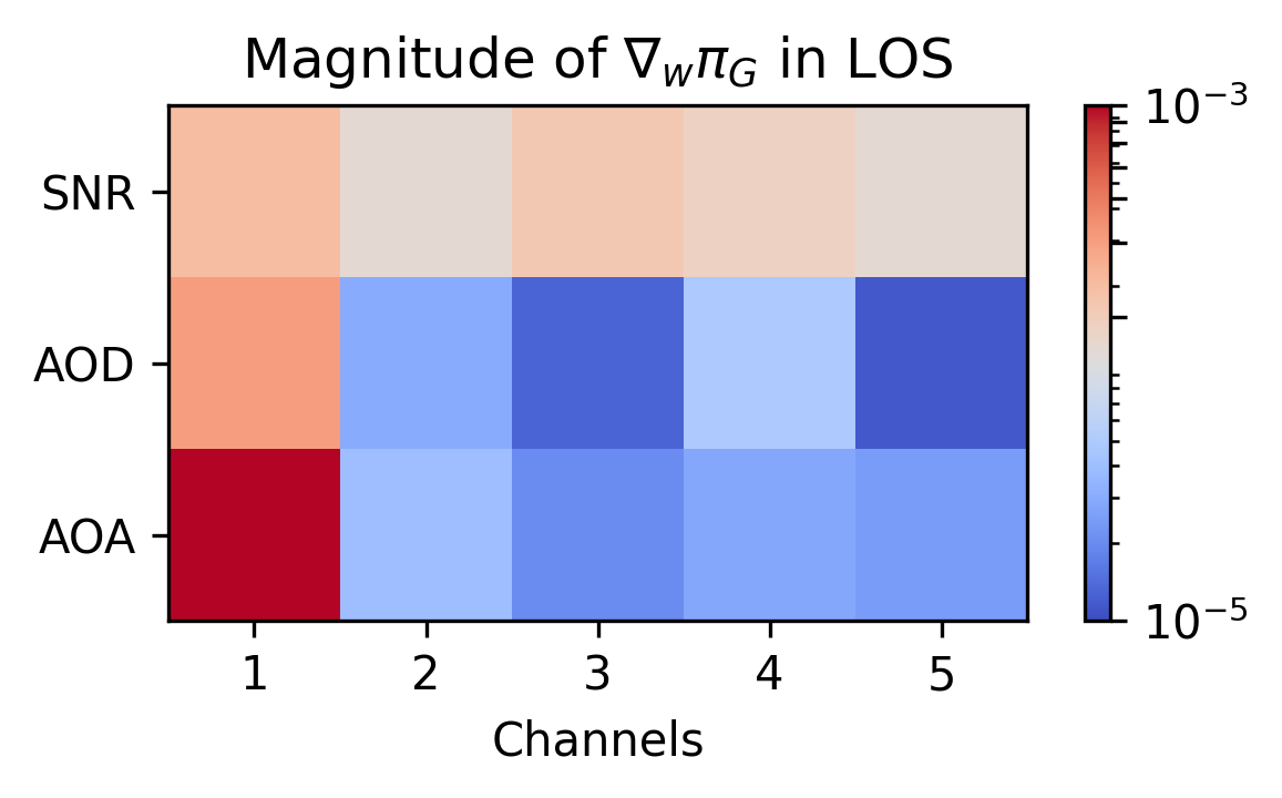
(d) In LOS, the PIRL policy output is mostly sensitive to the AoA of the first channel.

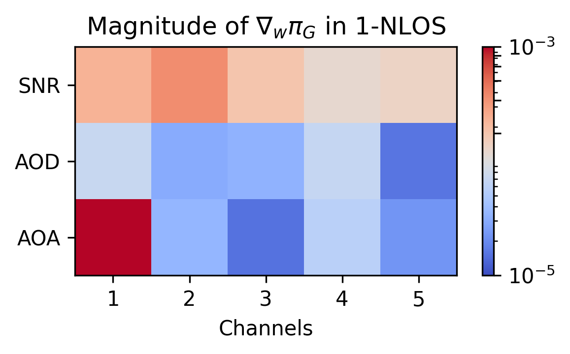
(e) In 1-NLOS, the PIRL policy output is mostly sensitive to the AoA of the first channel.

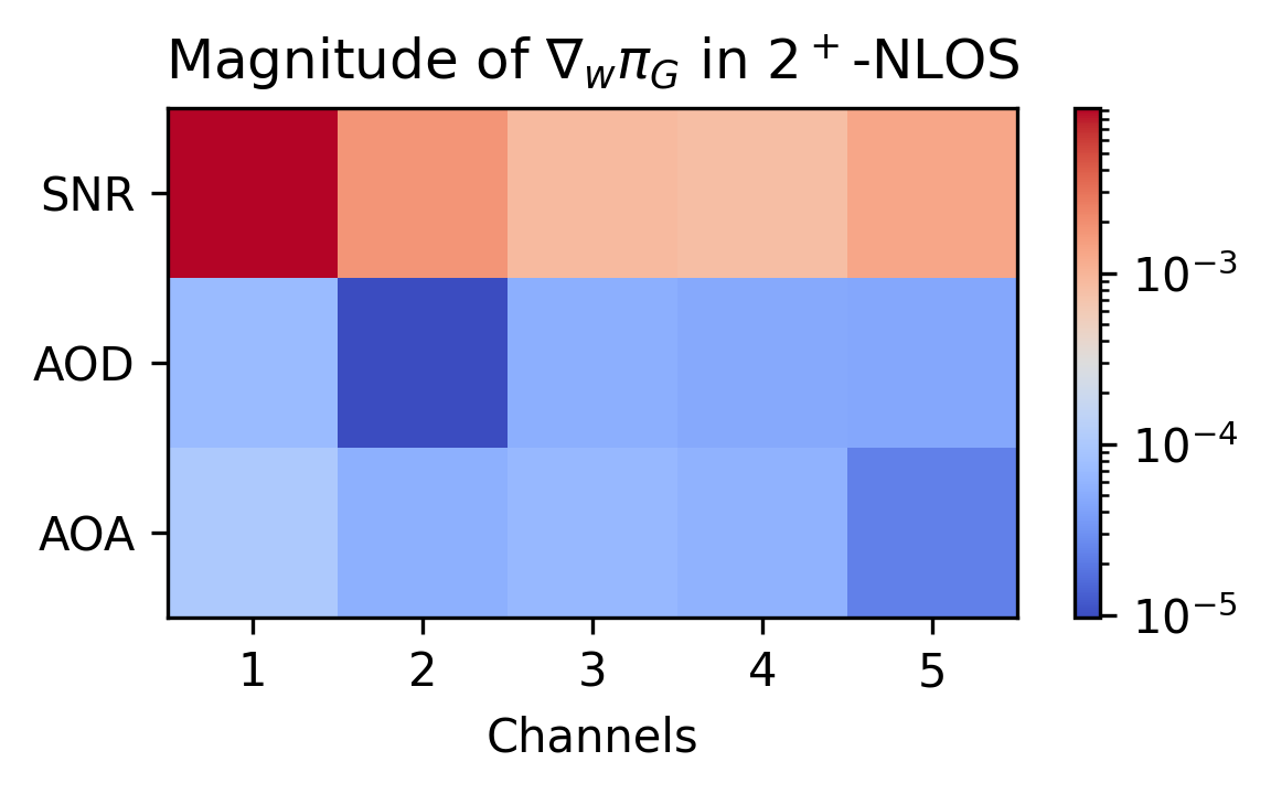
(f) In $2^{+}$-NLOS, the PIRL policy output is mostly sensitive to the SNR of the first channel.

Figure 6: The interpretability experiments on the reversibility principle and the SNR heuristic.

We provide empirical evidence that the PIRL leverages the principles stated in Section IV in the sense that the agent’s behavior is well aligned with the physics principles. Specifically, we focus on 1) the reversibility principle: whether the agent follows the AoA, and 2) the gradient heuristic: whether the agent moves toward the high-SNR direction. Figure 6(a), 6(b), and 6(c) present the histograms of 1000 sample angle outputs $\hat{\Omega}$ (i.e., moving directions) at a LOS, a 1-NLOS, and a $2^{+}$-NLOS position, respectively. One can see from these figures that the PIRL obeys the physics principles enforced by $C_{\rm AoA}$ and $C_{\rm SNR}$.

Furthermore, we attempt to interpret the PIRL model using explainable AI methodologies, such as LIME [12]. However, LIME aims to learn an interpretable model (e.g., decision trees) using perturbed training data as a surrogate to the original model. The perturbation is to highlight the features contributing the most to the output. The difficulty of applying LIME in WIN setup is that properly perturbing the wireless field is challenging. Due to diffractions and reflections in mmWave propagation, a slight offset to the target location can create drastically different wireless fields. Hence, as a compromise, we compute the gradient of the PIRL model regarding the input wireless data to inspect whether the instrumental features include AoA in LOS/1-NLOS and SNR in $2^{+}$-NLOS, as suggested by the physics principles. Figure 6(d), 6(e), and 6(f) empirical confirms that the PIRL model leverages the wireless information as instructed by the principles, which points to another advantage of incorporating the physics information into RL: the physics-based reward components lead to interpretable navigation.

Ablation Study

Recall that PIRL differs from WAN in its use of link state and SNR information. We conduct ablation studies regarding $C_{\rm LS}$ and $C_{\rm SNR}$, for which we report the NPL results. For the SNR ablation, we replace $C_{\rm SNR}$ with the relative distance cost in $2^{+}$-NLOS to see whether the SNR heuristic helps the agent navigate efficiently in such a scenario. As one can see from Table II, the answer to the question is affirmative, as the SNR ablation returns significantly higher NPLs in $2^{+}$-NLOS. We also replace $C_{\rm LS}$ with a constant number to investigate whether the link-state penalty discourages the agent from entering the higher-order NLOS area from the lower-order NLOS. The third row in Table II indicates that without $C_{\rm LS}$, the agent frequently revisits the high-order NLOS areas in testing, which yields higher NPLs in NLOS scenarios. In summary, $C_{\rm SNR}$ contributes to PIRL’s success in $2^{+}$-NLOS, and $C_{\rm LS}$ helps stabilize the navigation (less variance).

TABLE II: Ablation Studies on the SNR and link state terms. The metric is NPL averaged over all testing tasks.

	LOS	1-NLOS	$2^{+}$-NLOS
WAN	$1.01\pm 0.01$	$1.45\pm 0.03$	$3.83\pm 0.81$
PIRL	$1.01\pm 0.01$	$1.41\pm 0.03$	$2.60\pm 0.05$
SNR Ablation	$1.02\pm 0.02$	$1.46\pm 0.04$	$4.62\pm 1.15$
Link State Ablation	$1.02\pm 0.02$	$1.47\pm 0.05$	$3.90\pm 1.02$

VI Conclusion

This work develops a physics-informed RL (PIRL) for wireless indoor navigation. By incorporating physics prior into reward shaping, PIRL introduces learning biases to modulate the policy learning favoring those adhering to physics principles. As these principles are invariant across training/testing tasks, PIRL alleviates catastrophic forgetting in training and displays zero-shot generalization in testing.

Appendix A Related Works-Extended Discussion

Wireless Navigation and Localization

Emerging positioning technologies are increasingly leveraging the potential of Ultra-wideband (UWB) and high-frequency wireless bands such as millimeter waves, as underscored by prior research [27, 3, 4]. Traditional UWB positioning systems operating in these frequency bands yield a high temporal resolution, while densely packed, high-frequency radio bands and arrays attain remarkable angular resolution. A growing body of research and applications harness these wireless signals for indoor navigation. Feng et al. [7], for instance, developed an integrated indoor positioning system that enhances precision and robustness by merging Inertial Measurement Unit with UWB technology using Kalman filters. Their focus lies in optimizing the geometric distribution of base stations (BS) and minimizing the dilution of precision (DOP). In contrast, our study seeks to design a universally applicable navigation strategy for all signal strength ranges in indoor environments, relying on a singular BS. Similarly, Ayyalasomayajula et al. [8] unveiled a deep learning-aided wireless localization algorithm paired with an automated mapping platform, circumventing conventional RF-based localization techniques’ drawbacks. Their approach, however, requires pre-exploration and subsequent map generation. Our method, conversely, utilizes a physics-informed reinforcement learning model, built on a wireless digital twin, facilitating direct navigation in unexplored settings. Lastly, Yin et al. [5] probed into millimeter wave-based positioning for a target localization problem using a mobile robotic agent to capture mmWave signals. Their approach, integrating machine learning-based link state classification with a neural simultaneous localization and mapping (SLAM) module, heavily depends on the classification of the received wireless signal’s state. In contrast, our algorithm suggests the possibility of effective navigation using wireless signals, even in weaker link states.

Physics-informed RL

Reinforcement Learning, in particular, online RL[28], suffers from poor sample efficiency (either discrete [29] or continuous tasks [30]), especially when facing sophisticated tasks such as WIN. Physics-informed RL (PIRL) emerges as a promising remedy through integrating data and mathematical physics models. Even though no census has been established on the exact definition, PIRL amounts to introducing appropriate observational, inductive, and learning biases that can facilitate the learning process [13]. Introducing observation biases bears the same spirit of data augmentation, where the underlying physics law is embedded into the training data. For example, [16] trains an RL model using a combination of historic data and synthetic data generated from a traffic flow model for ramp metering. By incorporating into the RL training a predicted conflict zone visualized by a physics-based prediction algorithm, [15] develops a physics-informed aircraft conflict resolution strategy. Inductive biases correspond to interventions to the RL model architecture, and the resulting outputs are guaranteed to implicitly satisfy a set of given physics laws. One example is the physics-informed model-based RL considered in [31], where the physics constraints are imposed on the model learning. Our proposed PIRL-WIN method belongs to the third class: introducing learning biases. By selecting appropriate loss functions and constraints to modulate the training, this class of PIRL favors convergence to solutions adhering to the underlying physics. Similar to our physics-informed penalty, a reward-shaping mechanism is proposed in [14] for nuclear assembly design. To the best of our knowledge, this work is among the first endeavors to investigate the physics principles in the 5G wireless domain for RL-based indoor navigation.

Appendix B Physics Principles in WIN

This section provides further justification on the principles in Section IV. We begin with the proof of 1.

Proposition 1 (Monotonicity of Link States).

Given navigation path $\vec{p}:=(p_{1},\ldots,p_{H})$, $p_{t}$ denotes the pose at time $t$, let $\ell_{t}=\ell(p_{t})$ be the link state of the pose $p_{t}$. A necessary condition of $\vec{p}$ being the shortest path is that the link state $\ell$ is non-increasing along the path: $\ell_{i}\leq\ell_{j}$, for $0\leq j<i\leq H$.

Proof.

Consider a navigation path $\vec{p}:=(p_{1},\ldots,p_{H})$, $p_{t}$ denotes the pose at time $t$. Let $\ell_{t}=\ell(p_{t})$ be the corresponding link state of the pose $p_{t}$. Suppose, for the sake of contradiction, that for the shortest path $\vec{p}$, there exists $0\leq j<i\leq H$ such that $\ell_{i}>\ell_{j}$, and we consider two possible cases: 1) $\ell_{i}=1>0=\ell_{j}$, and 2) $\ell_{i}=2>1=\ell_{j}$. In the first case, when entering the LOS area, the agent shall remain in the LOS, as we discussed earlier. Hence, $\vec{p}$ is not optimal. In the second case, since $\ell$ cannot jump from 2 to 0, there must be some 1-NLOS after $p_{i}$. Let $k>i$ be the smallest index for which $\ell_{k}=1$, then connecting $\ell_{j}$ and $\ell_{k}$ yields a shorter path, conflicting the optimality. Figure 2(a) presents a visualization of the two cases. ∎

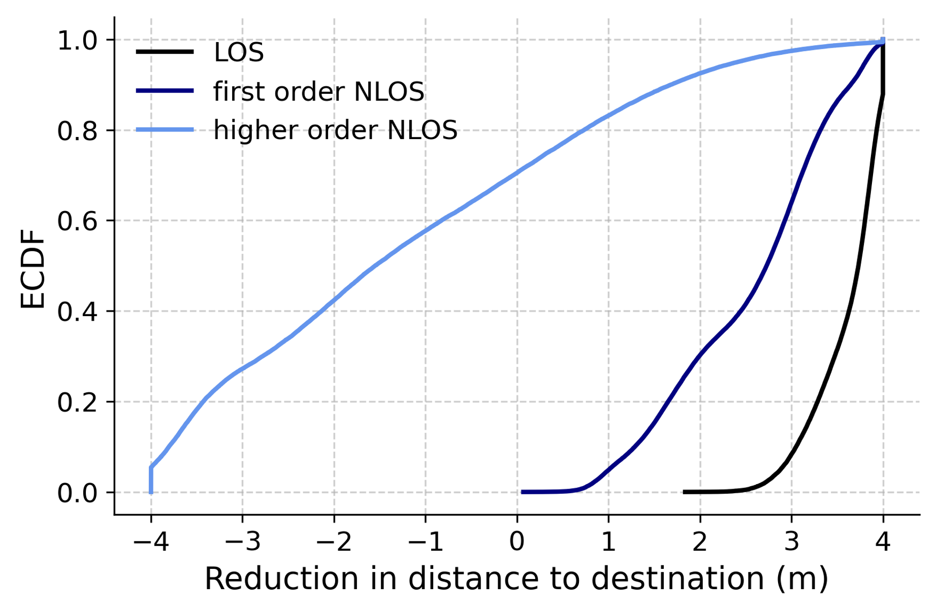
Figure 7: The reversibility principle leads to an effective navigation strategy.

To test the reversibility-based strategy, we selected 20 maps and pinpointed starting positions that were at least $4\text{\,}\mathrm{m}$ distant from the endpoint. For each initial position, a short-term goal was established $4\text{\,}\mathrm{m}$ away, aligned with the direction of the AoA. The robot was then directed towards the short-term goal, moving a distance of $4\text{\,}\mathrm{m}$, and the consequent reduction in distance to the endpoint was recorded. Figure 7 depicts the Empirical Cumulative Distribution Function (ECDF) for the decrease in distance to the target location. This illustration clearly shows that progression in the direction of the AoA effectively propels the robot closer to the endpoint when the initial link state is either LOS or 1-NLOS. In LOS scenarios, over 80% of instances facilitated the robot’s approach to the endpoint by more than $3.2\text{\,}\mathrm{m}$, while in 1-NLOS scenarios, a reduction of over $2\text{\,}\mathrm{m}$ was observed in 70% of the cases. Conversely, in $2^{+}$-NLOS scenarios, about 75% of instances resulted in the robot diverging further from the endpoint. Hence, the second physics-informed principle we put forth stipulates that the AoA can provide precise navigation guidance solely in LOS and 1-NLOS scenarios.

Appendix C Reinforcement Learning Algorithms

This section provides details about our reinforcement learning algorithms. We begin with introducing the global policy and the local policy, which directly controls the agent’s navigation.

C-A Hierarchical Structure

To accommodate the heterogeneous information (vision and wireless), we leverage the hierarchical structure of the RL policy in [18]. The RL policy consists of two separate neural networks, $\pi(\theta)=(\pi_{G}(\theta_{G}),\pi_{L}(\theta_{L}))$, where $\pi_{G}$ is a goal policy network that sets a long-term goal location, and $\pi_{L}$ is a local policy that navigates to the long-term goal. Similar to [5], we use wireless information for the goal policy. Specifically, the goal policy takes as inputs $\alpha_{t}=(\hat{\Omega}_{t},\hat{\ell}_{t})$ a pair of an estimated angle and link-state estimates based on the current wireless input $w_{t}$. As its name suggests, $\hat{\ell}_{t}$ is the agent’s estimate of the current link state, while $\hat{\Omega}_{t}$ is the estimate of the relative angle of the target position to the current pose. The two estimates lead to a conjectured target position, referred to as the long-term goal, which is then fed into a planner, together with the spatial map $m_{t}$ and the pose estimate $\hat{p}_{t}$ from the SLAM module. The planner, based on the Fast Marching method [32], computes the shortest path from the current location to the conjectured target. The local policy takes in the path-planning output and the camera images, producing navigation actions $a_{t}\in\mathcal{A}$ for collision avoidance. To streamline our training process, we load a pre-trained local policy and only train the global one. A schematic illustration is presented in Figure 8.

Figure 8: The hierarchical structure of the RL policy. The global policy takes in the wireless input and produce predicted target position. The local policy convert the prediction into a sequence of navigation actions.

C-B Global Policy Algorithm

Given the global policy output $\alpha_{t}$ and the agent current pose estimate $\hat{x}_{t},\hat{y}_{t}$, the long-term goal $p^{L}_{t}=(x^{L}_{t},y^{L}_{t})$ is given by $x^{L}_{t}=\hat{x}_{t}+\delta_{t}\cos{\hat{\Omega}_{t}}$, $y^{L}_{t}=\hat{y}_{t}+\delta_{t}\sin{\hat{\Omega}_{t}}$, where $\delta_{t}$ is a predicted distance depending on the link state conjecture $\hat{\ell}_{t}$. The predicted distance is given by $\delta_{t}=\mathds{1}_{\{\hat{\ell}_{t}=2\}}\cdot D_{b}+(1-\mathds{1}_{\{\hat{\ell}_{t}=2\}})\cdot D_{s}$, where $D_{b}=7.5$ leading to aggressive exploration and $D_{s}=2.5$ to a conservative one. The intuition behind this setting is as follows: if the agent is in a state of $2^{+}$-NLOS, it prefers to search for the goal aggressively; if not, the agent prefers to move slowly, being more cautious.

Global Reward Design

In the numerical implementations, the reward function in the training phase is different from the summation of all physics-motivated terms described in Section IV. To further enforce the monotonicity of link states in the LOS and 1-NLOS, the global reward function design is as follows. If the link state is LOS or 1-NLOS, the cost is given by $r^{g}_{t}=\lambda_{\rm LS}C_{\rm LS}\cdot(\zeta_{1}e^{-\zeta_{2}c_{t}}-\lambda_{\rm AoA}C_{\rm AoA})$; otherwise, if exploring the $2^{+}$-NLOS, the reward function is given by $r^{g}=-\lambda_{\rm SNR}C_{\rm SNR}$. Here, $\zeta_{1}$ and $\zeta_{2}$ are hyperparameters. For our experiments, we set the values as follows: $\lambda_{\rm LS}=1.1,\lambda_{\rm AoA}=1.0,\lambda_{\rm SNR}=1.2,\zeta_{1}=600$, and $\zeta_{2}=0.1$. For the SNR cost $C_{\rm SNR}$, the relative angle $\nu_{t}$ is specified as follows. Consider a discretization of the angle range $\{-180,-170,\ldots,0,\ldots,170,180\}$. For each relative angle from the discrete set, we compute the average of SNR evaluations at all mesh points (where the wireless data is collected, see Appendix F) along the direction. The highest SNR direction is set to be $\nu_{t}$.

PPO

Denoting $G_{t}=\sum^{H}_{k=0}\gamma^{k}r^{g}_{t+k+1}$ as the discounted future reward, we can now derive the value of state $w$ when following a policy $\pi$ as $V^{\pi}(w)=\mathbb{E}_{\alpha\sim\pi}\left[G_{t}|W_{t}=w\right]$. Similarly, we can determine the value of a (state, action) pair when following the policy $\pi$ as $Q^{\pi}(w,\alpha)=\mathbb{E}_{\alpha\sim\pi}\left[G_{t}|W_{t}=w,A_{t}=\alpha\right]$, where $\mathbb{E}_{\alpha\sim\pi}$ denotes the expectation over the action $\alpha$ sampled from the policy $\pi$. To measure the performance of an action within a certain state, we use the advantage function as follows $A^{\pi}(w,\alpha)=Q^{\pi}(w,\alpha)-V^{\pi}(w)$.

In the PPO algorithm, a clipped surrogate objective is used as a constraint. Let $\pi_{\theta_{\text{old }}}$ represent the old policy, and $\pi_{\theta}$ denote the new policy. The probability ratio is denoted as $\mu(\theta)=\frac{\pi_{\theta}(\alpha|w)}{\pi_{\theta_{\text{old }}}(\alpha|w)}$. Additionally, we introduce a small hyperparameter $\epsilon$. To ensure the ratio remains within a certain range, we define the clipping function as $\mbox{clip}(\mu(\theta),1-\epsilon,1+\epsilon)$. This function restricts the ratio to be no greater than $1+\epsilon$ and no less than $1-\epsilon$. Therefore, the objective function for this clipping is:

$$\begin{split}J^{\mathrm{CLIP}}(\theta)&=\mathbb{E}\left[\min\left(\mu(\theta)\hat{A}_{\theta_{\text{old }}}(w,\alpha),\right.\right.\left.\left.\operatorname{clip}(\mu(\theta),1-\epsilon,1+\epsilon)\hat{A}_{\theta_{\text{old }}}(w,\alpha)\right)\right].\end{split}$$

Here, $\hat{A}_{\theta_{\text{old }}}(\cdot)$ represents the estimated advantage for the old policy. The objective function $J^{\mathrm{CLIP}}(\theta)$ calculates the expectation over the minimum value between two terms: the first term is the product of the ratio and the estimated advantage under the old policy, while the second term is the product of the clipped ratio and the estimated advantage under the old policy, which means the policy loses its motivation for increasing the update to extremes for better rewards.

When implementing PPO on a network architecture with shared parameters for both the policy (actor) and value (critic) functions, the critic is responsible for updating the value function to obtain the estimated advantage function $\hat{A}_{\theta_{\text{old }}}(\cdot)$. On the other hand, the actor serves as our policy model.

To promote sufficient exploration in the learning process, an error term and an entropy bonus is introduced for value estimation and exploration encouragement, denoted as $(V_{\theta}-V_{\text{target}})^{2}$ and $H(w,\pi_{\theta}(\alpha|w))$. Here, $V_{\text{target}}$ represents the discounted cumulative reward associated with the observations made throughout an experienced trajectory. When a given trajectory ends, target state values are computed for each state $p_{t}$ encountered during the trajectory using the following equation:

$$\begin{split}V_{t}^{\text{target }}&=r_{t}+\gamma r_{t+1}+\gamma^{2}r_{t+2}+\ldots+\gamma^{k-1}r_{t+k-1}+\gamma^{n}V_{\theta_{\text{old }}}\left(w_{t+k}\right).\end{split}$$

Therefore, the overall PPO objective function can be written by:

$$\begin{split}J^{\mathrm{PPO}}(\theta)&=\mathbb{E}\left[J^{\mathrm{CLIP}}(\theta)-\xi_{1}(V_{\theta}-V_{\text{target}})^{2}\right.\left.+\xi_{2}H(p,\pi_{\theta}(\alpha|w))\right].\end{split}$$

where $\xi_{1}$ and $\xi_{2}$ are two hyperparameter constants equals to $0.5$ and $0.02$. By optimizing the objective function $J^{\mathrm{PPO}}(\theta)$, we can find the optimal policy $\pi$.

C-C Local Policy Algorithm

The local policy takes in the RGB observation $v_{t}$ and the short-term goal $p^{S}_{t}$, where the short-term goal is derived by the planner $f_{plan}$: $p_{t}^{S}=f_{plan}(p^{L}_{t},m_{t},\hat{p}_{t})$. Then, the local output is $\mathcal{A}_{t}=\pi_{L}(v_{t},p_{t}^{S}|\theta_{L})$. The reward is determined by the agent’s proximity to the short-term objective, and the cross-entropy loss is utilized. The Local Policy undergoes training via imitation learning, specifically through behavioral cloning. For more details on the planner and the local policy, please refer to [18].

C-D Architecture of the Global and the Local Policies

The global policy comprises a recurrent neural network architecture, which includes a linear sequential wireless encoder network with two layers, followed by fully connected layers and a Gated Recurrent Unit (GRU) layer [33]. Additionally, there are two distinct layers at the end, referred to as the actor output layer and the critic output layer. The local policy is constructed using a recurrent neural network architecture. It incorporates a pre-trained ResNet18 [34] as the visual encoder, which is followed by fully connected layers and a GRU layer.

C-E PIRL Policy Algorithm

From our discussions above and in the main text, the global policy and the local policy operate on the same time scale. However, in practical training scenarios, this synchronicity setting proves to be inappropriate due to computational resource constraints, and the physical movement constraints of the agent (i.e., the agent requires at least 5 steps to turn around). Consequently, we introduce a new time variable $\eta$ defined as $t=H_{l}\eta$, where $H_{l}\in\mathbb{R}$ represents the time horizon for the local policy. Consequently, we now have two distinct time variables, namely $t$ and $\tau$, corresponding to the global and local policies, respectively. This implies that global and local policies operate on different time scales. Then we can write the pseudocode outlining the PIRL policy shown in algorithm 1.

Algorithm 1 PIRL Algorithm

1:Global policy $\pi_{G}$, pre-trained Local policy $\pi_{L}$, and the planner module $f_{PLAN}$; Time horizon $H_{g},H_{l}$

2:Initialize global policy parameters $\theta_{0}$;

3:while not converged do

4:     Reset environment and agent state;

5:     Set global time $t=0$;

6:     Sample initial time $w_{t},v_{t}$ for policies;

7:     while $t<H_{g}$ do

8:         Set local time $\tau=0$;

9:         Sample action $\alpha_{t}$ from global policy $\pi_{G}(w_{t}|\theta)$;

10:         Compute long-term goal $p_{t}^{L}$ using $\alpha_{t}$;

11:         Compute short-term goal $p_{t}^{S}$ using planner $f_{PLAN}$;

12:         while $\tau<H_{l}$ do

13:              Sample action set $a_{l}$ from local policy $\pi_{L}(v_{t},p_{t}^{S})$;

14:              Execute action $a_{l}$ and observe next state $v_{\tau+1}$;

15:              Update local time $\tau=\tau+1$;          

16:         Update global policy parameter $\theta$ using collected data and the PPO algorithm in C-B;

17:         Observe next state $w_{t+1}$;

18:         Update global time $t=t+1$;      

19:Output $\theta_{t}$

Appendix D Experiment Setup

TABLE III: Label-Map Correspondence

Label	Map Name	Label	Map Name	Label	Map Name
A	Bowlus	I	Capistrano	P	Woonsocket
B	Arkansaw	J	Delton	Q	Dryville
C	Andrian	K	Bolton	R	Dunmor
D	Anaheim	L	Goffs	S	Hambleton
E	Andover	M	Hainesburg	T	Colebrook
F	Annawan	N	Kerrtown	U	Hometown
G	Azusa	O	Micanopy
H	Ballou

Table LABEL:tab:label_map presents the label map correspondence, where the left-hand side displays the maps used for training, while the right-hand side displays the maps used for testing. During the training phase, the first 15 maps $(A-O)$ with associated 10 task positions are utilized to learn a PIRL policy in sequential order. The training process follows a specific sequence, starting with task $A1$ and progressing to $A10$, followed by training under tasks $B1$ to $B10$. Each task consists of 1000 training episodes. This procedure is repeated until the agent has been exposed to all 15 maps with all target positions. The intuition behind this sequential training approach is to gradually increase the complexity of the tasks. It begins with LOS cases, which are relatively simple, then proceeds to 1-NLOS cases, and finally to $2^{+}$-NLOS cases, which pose a higher level of difficulty. Depending on the task, we use different learning rates on LOS, 1-NLOS, and $2^{+}$-NLOS which are $1\text{e}^{-4},1\text{e}^{-5},\text{ and }1\text{e}^{-6}$. For the global horizon $H_{g}$, we choose $10$, and for the local horizon $H_{l}$, we choose $20$.

In contrast to the sequential training of PIRL, we apply rotation training to NPRL, as it suffers from catastrophic forgetting. The rotation training generally follows the task sequence as the sequential training. Yet, after finishing the training on the current task, we randomly select a set of previous tasks to re-train the model before moving to the next task in the sequence to refresh NPRL’s “memory”. The number of re-train tasks is set to be half of the total number of finished tasks.

The remaining 6 maps ($P$ to $U$) are reserved for testing purposes. A total of 20 repeated tests with different random seeds are conducted. For each map, we collect 200 NPLs obtained from these different random seed tests and obtain their average.

Appendix E Extended Experiment Results

E-A Generalization

To make the comparison results less overwhelming, for each testing map, we only report the three average NPLs over LOS tasks (e.g., the average NPL over P1-3), 1-NLOS tasks (e.g., the average NPL over P4-6), and $2^{+}$-NLOS (e.g., the average NPL over P7-10), respectively. The results are presented in Table IV. Our PIRL policy generalizes well to these unseen tasks and achieves the smallest NPLs across all three scenarios, compared with baselines. In particular, we highlight the efficient navigation of PIRL in $2^{+}$-NLOS, the most challenging case, where the NPL is remarkably smaller than NPRL. Note that the horizon length is fixed and the upper bound of NPL is around 5 to 6 (depending on the map). The NPLs of NPRL and V-SLAM in $2^{+}$-NLOS imply that the agent fails to reach the target within the horizon in a large number of testing cases, demonstrating the superiority of PIRL.

TABLE IV: A comparison of NPLs under 6 testing maps. PIRL achieves impressively efficient navigation in the challenging scenario $2^{+}$-NLOS, compared with baselines.

	Map P			Map Q			Map R
	LOS	1-NLOS	$2^{+}$-NLOS	LOS	1-NLOS	$2^{+}$-NLOS	LOS	1-NLOS	$2^{+}$-NLOS
PIRL	1.01 $\pm$ 0.01	1.31 $\pm$ 0.02	2.53 $\pm$ 0.05	1.01 $\pm$ 0.01	1.50 $\pm$ 0.04	2.61 $\pm$ 0.05	1.01 $\pm$ 0.00	1.23 $\pm$ 0.03	2.55 $\pm$ 0.06
NPRL	2.03 $\pm$ 1.02	2.72 $\pm$ 0.55	4.96 $\pm$ 1.37	2.12 $\pm$ 1.00	3.08 $\pm$ 0.68	5.00 $\pm$ 1.41	2.28 $\pm$ 1.03	2.49 $\pm$ 0.81	4.99 $\pm$ 1.20
V-SLAM	1.05 $\pm$ 0.02	1.82 $\pm$ 0.51	4.58 $\pm$ 1.12	1.11 $\pm$ 0.03	2.89 $\pm$ 0.73	4.89 $\pm$ 1.00	1.09 $\pm$ 0.03	1.68 $\pm$ 0.6	4.68 $\pm$ 1.01
WAN	1.02 $\pm$ 0.00	1.32 $\pm$ 0.02	3.88 $\pm$ 0.82	1.01 $\pm$ 0.01	1.63 $\pm$ 0.05	3.71 $\pm$ 0.71	1.01 $\pm$ 0.00	1.23 $\pm$ 0.02	3.97 $\pm$ 0.83
	Map S			Map T			Map U
	LOS	1-NLOS	$2^{+}$-NLOS	LOS	1-NLOS	$2^{+}$-NLOS	LOS	1-NLOS	$2^{+}$-NLOS
PIRL	1.01 $\pm$ 0.01	1.23 $\pm$ 0.01	2.82 $\pm$ 0.04	1.00 $\pm$ 0.00	1.43 $\pm$ 0.03	2.59 $\pm$ 0.06	1.01 $\pm$ 0.01	1.73 $\pm$ 0.03	2.46 $\pm$ 0.05
NPRL	2.01 $\pm$ 0.99	2.81 $\pm$ 0.83	5.14 $\pm$ 1.21	2.23 $\pm$ 1.10	3.13 $\pm$ 0.83	4.88 $\pm$ 1.86	1.90 $\pm$ 0.89	3.25 $\pm$ 0.64	4.50 $\pm$ 1.05
V-SLAM	1.04 $\pm$ 0.03	1.99 $\pm$ 0.58	4.98 $\pm$ 1.00	1.10 $\pm$ 0.08	3.01 $\pm$ 0.67	4.69 $\pm$ 1.01	1.06 $\pm$ 0.04	3.19 $\pm$ 0.56	4.43 $\pm$ 1.00
WAN	1.01 $\pm$ 0.00	1.32 $\pm$ 0.03	3.78 $\pm$ 0.90	1.00 $\pm$ 0.00	1.48 $\pm$ 0.02	4.01 $\pm$ 0.90	1.01 $\pm$ 0.01	1.74 $\pm$ 0.04	3.63 $\pm$ 0.70

To further investigate the knowledge transfer in the training phase, we propose a testing-while-training(TWT) procedure: the policy trained on the previous task is first tested on the current task, and after the testing, the training on the current task begins. The procedure repeats until the end of training. As shown in Figure 9, the overall trend of the NPL for PIRL is gradually decreasing as the training proceeds, even though it slightly increases when the task switch from the LOS to the NLOS (e.g., from $A3$ to $A4$ and $A7$) since navigating in the NLOS is inherently more challenging than in the LOS. In contrast, the NPLs for NPRL on different tasks are similar without significant improvements.

Figure 9: A summary of TWT results in the training phase.

E-B Explainability

This section provides an alternative viewpoint on the sensitivity analysis presented in the experiment section.

Suppose an Oracle, knowing the ground truth $(p_{t},o_{t})$, adheres to the physics principles for navigation using the wireless input $w_{t}$, and the resulting policy is denoted by $\pi_{physics}(w_{t})$. In the WIN context, $\pi_{physics}$ strictly follows the AoA in the LOS and 1-NLOS, while moves along the ascent direction of SNR. We propose the $n$-th order consistency test below, which is inspired by the function approximation and representation theory [35, 36]. The intuition is that the larger $n$ is, for which the equation $\nabla^{n}\pi_{physics}(w)=\nabla^{n}\pi_{G}(w)$ holds for a set of sample input $w$, the more likely the two functions coincide on the whole domain (for every possible $w$). This is because the error term in Taylor expansion decreases, as the order increases. Taking this inspiration, we put forth the consistency test. $\pi_{G}$ is said to be zeroth(first)-order consistent with $\pi_{physics}$ at the sample $w$ if $\pi_{G}(w)$ ($\nabla_{w}\pi_{G}$) is compatible with $\pi_{physics}$ ($\nabla_{w}\pi_{physics}$), meaning that the two display similar behaviors at $w$. This compatibility is more of a case-by-case discussion. For example, Figure (6(a))(6(b)) demonstrates the zeroth-order consistency, where the PIRL agent chooses angles close to first-channel AoA with high probabilities in the LOS and 1-NLOS ($\pi_{physics}$ chooses the AoA with probability 1). The first-order consistency is confirmed in Figure (6(d))(6(e)), where the absolute value of the partial derivative with respect to the first-channel AoA is the most significant among others ($\pi_{physics}$ only uses the AoA, hence all of its partial derivatives is zero, except the one on the AoA). Similar consistency results also hold for the SNR heuristic, where PIRL relies on the first-channel SNR. All the tests above are conducted at three representative points in a testing map. The consistency tests above offer empirical evidence that the PIRL agent acquires the physics knowledge and applies it to unseen tasks. Figure 10 present the three representative points mentioned in Figure 6. Figure 11 presents the average results of the first-order consistency test on ten locations within the map shown in Figure 10.

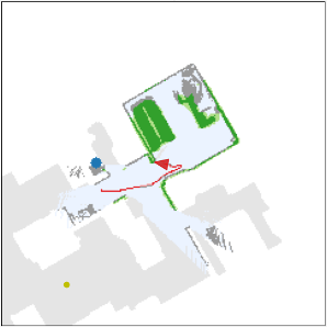
Figure 10: (a)(b)(c) shows the representative points in the LOS, 1-NLOS, and 2-NLOS, respectively, at which the consistency tests are conducted. The red triangle is the agent, the blue point is the long-term goal output by the global policy, and the green point is the target.

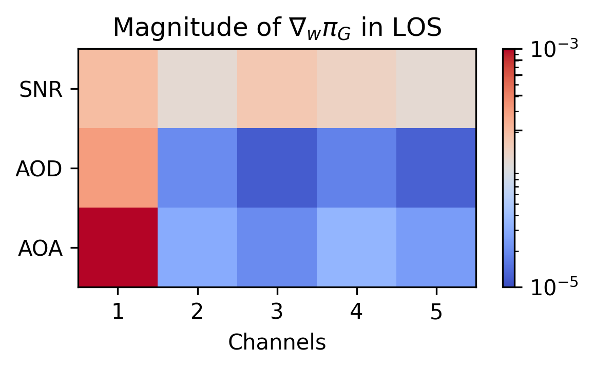
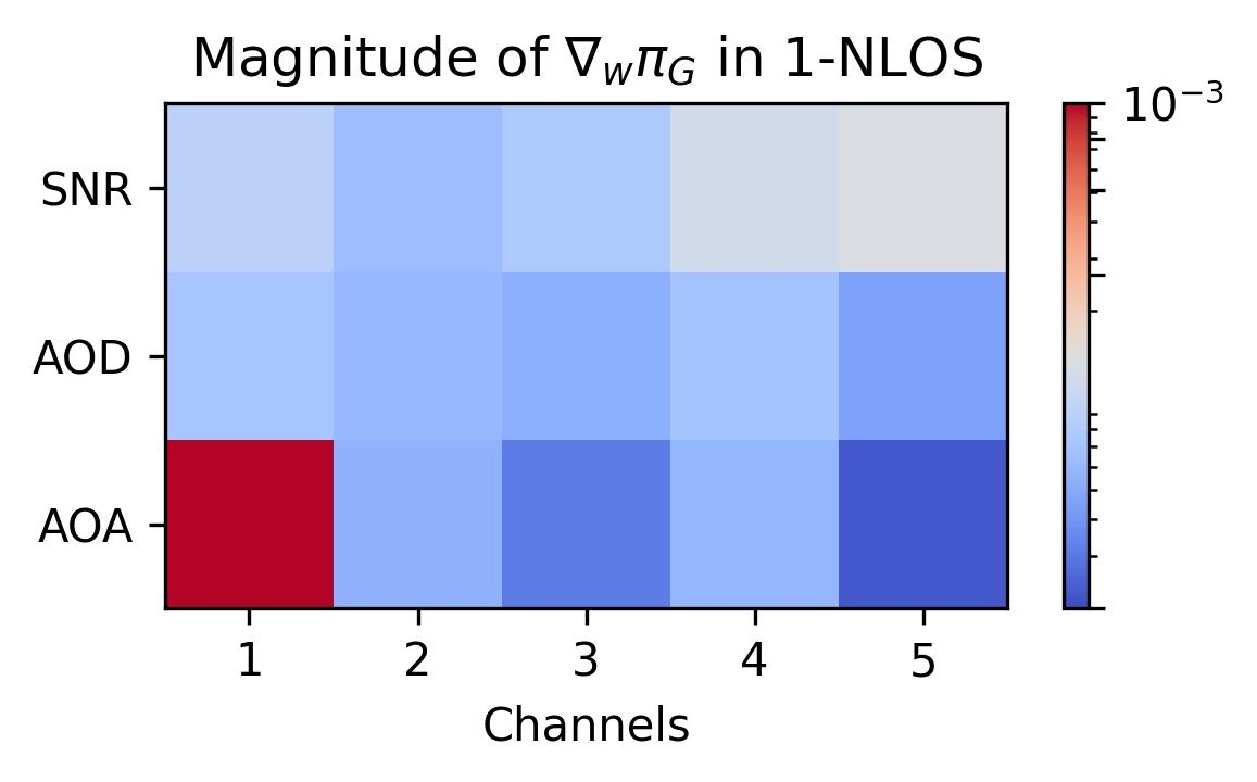
Figure 11: The average absolute value of $\nabla_{w}\pi_{G}$ at ten random locations in the map shown in Figure 10.

Appendix F Wireless Information and Wireless Digital Twin

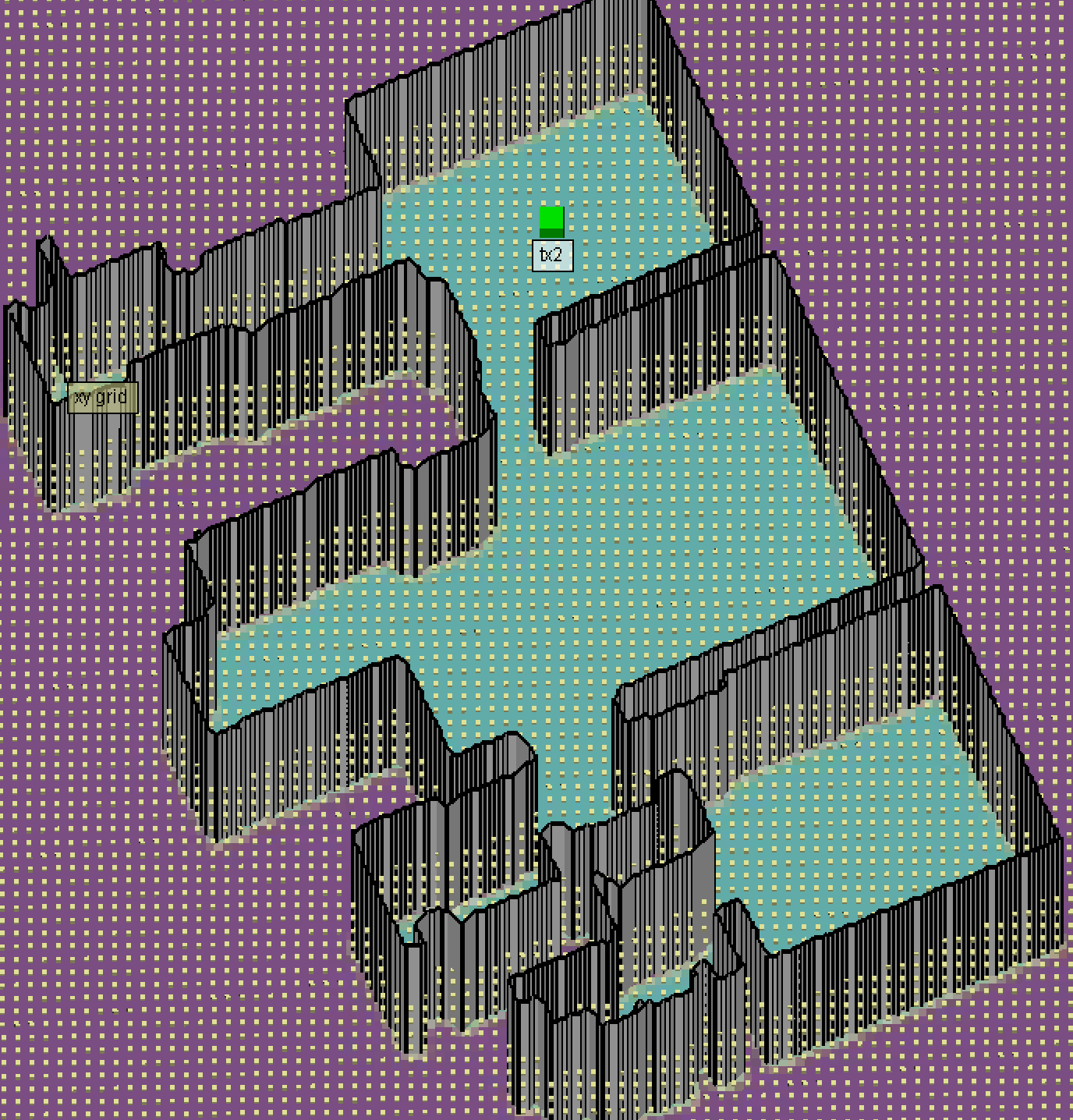
(a) Receiver grid demo.

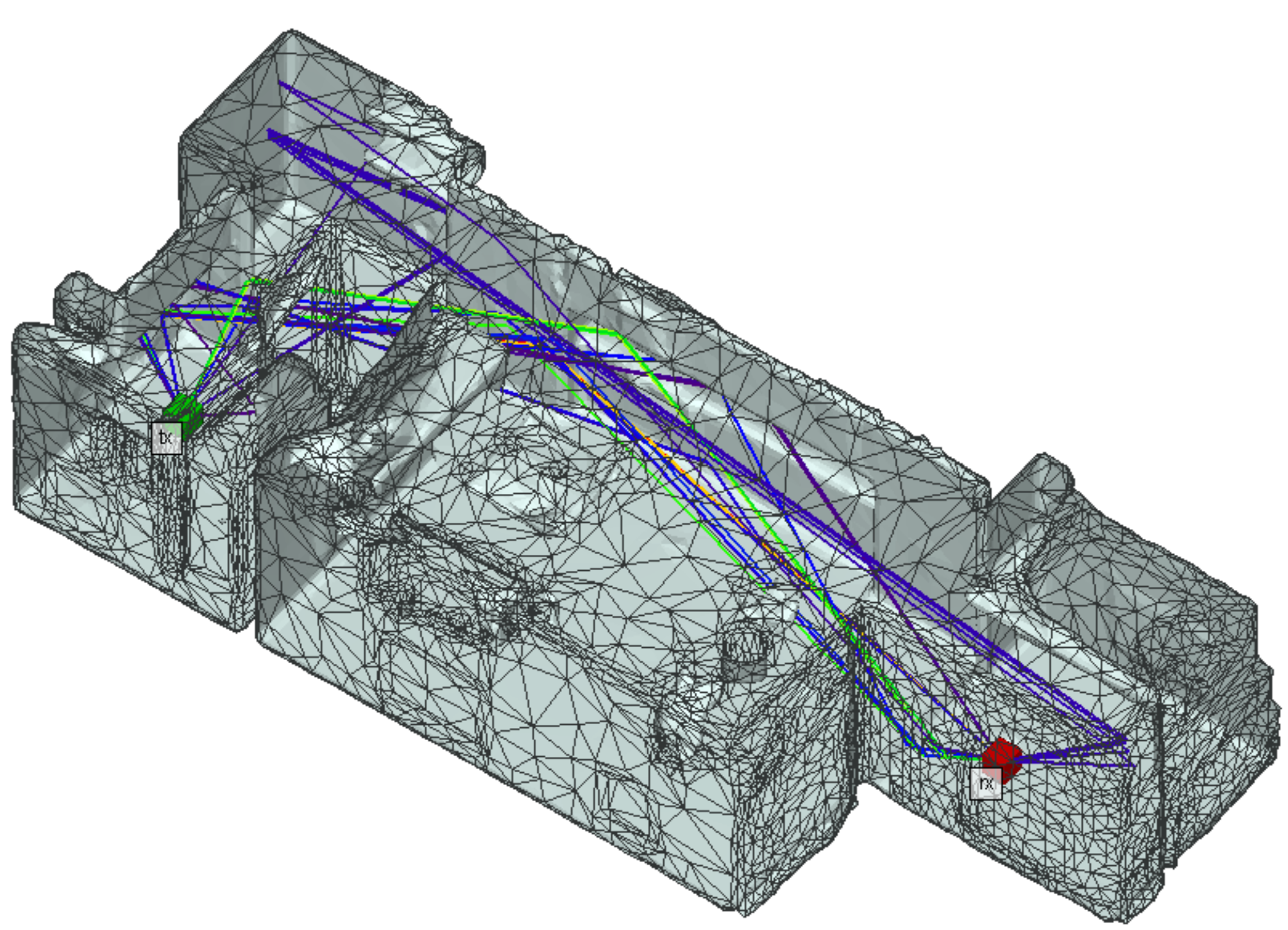
(b) Wireless link in ray tracing demo.

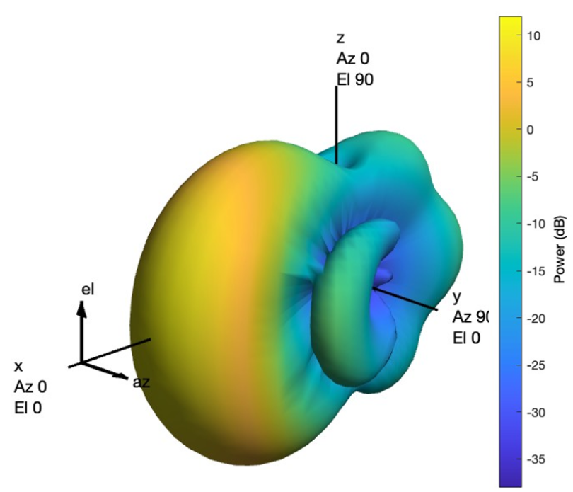
(c) Antenna pattern demo

Figure 12: Wireless Channel Simulation Demos

Wireless Information: Since wireless signals and RGB images are multi-dimensional vectors associated with the agent’s pose, the two can be treated as vector fields within the indoor environment, referred to as the wireless field $W(p)$ and the vision field $V(p)$, respectively. For each pose $p$, the wireless field $W(p)$ describes the wireless signal received by the agent at the pose $p$, which includes the angle of arrival (AoA) and departure (AoD) for five channels. AoA is the direction from which a wireless signal arrives at a receiving antenna. AoD is the direction in which a wireless signal departs from a transmitting antenna. Several wireless methods are available to estimate paths from transmitted signals; we use a tensor decomposition method from [5] reviewed below in Wireless Digital Twin. Mathematically, $W(p)=(g_{n},\Omega_{n}^{rx},\Omega_{n}^{tx})_{n=1}^{N}\in\mathbb{R}^{3\times N}$, where $N$ is the maximum number of detected paths, and, for path $n$, $g_{n}$ denotes its signal-to-noise ratio (SNR), $\Omega_{n}^{rx}$ and $\Omega_{n}^{tx}$ denote the AoA and AoD, respectively. Following [5], we use the top $N=5$ paths.

Wireless Digital Twins: The genesis of Wireless Digital Twins (WDTs) relies upon the Gibson model [37], a remarkable embodiment of real-world indoor reconstruction based on point clouds and RGB-D cameras. The realism of the RGB input $v_{t}$ in WDT surpasses that of the synthetic SUNCG dataset, earlier utilized in exploration research [38]. The simulated wireless field $W(p)$ adheres to the millimeter-wave (mmWave) simulation methodology expounded in [5].

To initiate the wireless data simulation, a mesh discretization of the 2D map with a cell width of $15\text{\,}\mathrm{c}\mathrm{m}$ is implemented, and wireless signals for each vertex point are generated. The simulation commences with the utilization of ray-tracing software such as Wireless InSite [39] to generate noise-free electromagnetic wave rays, as shown in 12(b). However, it is crucial to understand that these ray tracing wireless propagation paths are not an exact representation of real-world wireless channels that a robot could receive. That is to say, the robot cannot directly access the ray tracing paths in the real world, indicating a potential deviation between the simulated and real-world environments.

The subsequent phase involves the orchestration of antenna arrays, the induction of noise, and the subsequent disintegration of the channel, enabling the extraction of potential real-world robot receivable wireless signal paths.

The rendering of high-resolution ray-tracing data to cover the entire map for channel sounding and robot navigation entails the use of a 2D receiver (RX) grid with a $15\text{\,}\mathrm{c}\mathrm{m}$ interval, as shown in 12(a). Each task configuration includes one transmitter (TX) and a RX grid, referred to as a wireless link in wireless communication parlance. The strongest 25 rays out of 250 are chosen for each wireless link to simulate the wireless channel, as validated by numerous experiments [40, 41, 42].

The subsequent step involves the design of antenna arrays. Leveraging the theoretical foundations laid out in [43], a 1x8 patch microstrip antenna array for the RX and a 2x4 patch microstrip antenna array for the TX are simulated. These arrays enable effective beamforming, a process that involves the manipulation of phase and amplitude of signals from multiple antennas to concentrate signal power in specific directions. To ensure 360° coverage, three antenna arrays with azimuth angles 0°, 120°, and -120° and 0° elevation are deployed. To facilitate TX and RX detection, a known synchronization signal is transmitted by the TX, sweeping through a sequence of directions from the different TX arrays.

A 3D codebook of the mmWave system is designed following [44, 45] to obtain corresponding AoA and AoD in the channel decomposition post-medium wave. At this point, ray tracing data, antenna patterns, antenna group design, beamforming, and the codebook coalesce to simulate realistic indoor wireless channels. Notably, a loss of 6dB, inclusive of noise figures, is introduced during antenna group design, and additive white Gaussian noise (AWGN) assumed to be independent and identically distributed (i.i.d.) is added across the channel modeling RX antennas.

With the wireless channel acquired, the next step involves sub-channel (wireless path) estimation via low-rank tensor decomposition [46, 47]. This yields the wireless data $W(p)=(g_{n},\Omega_{n}^{rx},\Omega_{n}^{tx})_{n=1}^{5}\in\mathbb{R}^{3\times 5}$, where $g_{n}$ denotes the signal-to-noise ratio (SNR) of the $n$-th channel, and $\Omega_{n}^{rx}$ and $\Omega_{n}^{tx}$ denote the AoA and AoD of the $n$-th sub-channel.

Finally, the fusion of the wireless channel data with the Gibson indoor model culminates in the creation of WDTs, meticulously tailored for indoor navigation, as shwon in 13. For additional details regarding the simulation process, readers may refer to the pertinent sections in [5].

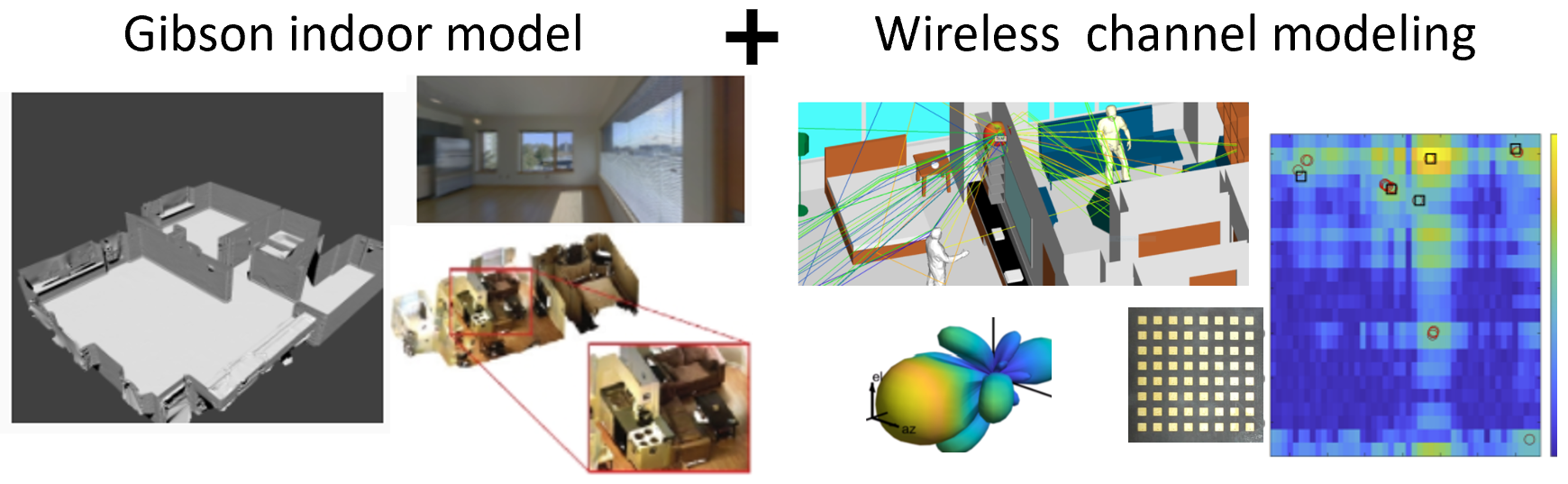
Figure 13: A summary of wireless digital twin (WDT)

References

[1]
S. Rangan, T. S. Rappaport, and E. Erkip, “Millimeter-wave cellular wireless
networks: Potentials and challenges,” Proceedings of the IEEE, vol.
102, no. 3, pp. 366–385, 2014.
[2]
E. Dahlman, S. Parkvall, and J. Skold, 5G NR: The next generation
wireless access technology. Academic
Press, 2020.
[3]
A. Shahmansoori, G. E. Garcia, G. Destino, G. Seco-Granados, and H. Wymeersch,
“5g position and orientation estimation through millimeter wave mimo,” in
2015 IEEE Globecom Workshops (GC Wkshps). IEEE, 2015, pp. 1–6.
[4]
F. Guidi, A. Guerra, and D. Dardari, “Millimeter-wave massive arrays for
indoor slam,” in 2014 IEEE International Conference on Communications
Workshops (ICC). IEEE, 2014, pp.
114–120.
[5]
M. Yin, A. K. Veldanda, A. Trivedi, J. Zhang, K. Pfeiffer, Y. Hu, S. Garg,
E. Erkip, L. Righetti, and S. Rangan, “Millimeter wave wireless assisted
robot navigation with link state classification,” IEEE Open Journal of
the Communications Society, vol. 3, pp. 493–507, 2022.
[6]
H. Surmann, C. Jestel, R. Marchel, F. Musberg, H. Elhadj, and M. Ardani, “Deep
reinforcement learning for real autonomous mobile robot navigation in indoor
environments,” arXiv preprint arXiv:2005.13857, 2020.
[7]
D. Feng, C. Wang, C. He, Y. Zhuang, and X.-G. Xia, “Kalman-filter-based
integration of imu and uwb for high-accuracy indoor positioning and
navigation,” IEEE Internet of Things Journal, vol. 7, no. 4, pp.
3133–3146, 2020.
[8]
R. Ayyalasomayajula, A. Arun, C. Wu, S. Sharma, A. R. Sethi, D. Vasisht, and
D. Bharadia, “Deep learning based wireless localization for indoor
navigation,” in Proceedings of the 26th Annual International
Conference on Mobile Computing and Networking, 2020, pp. 1–14.
[9]
T. S. Rappaport, R. W. Heath Jr, R. C. Daniels, and J. N. Murdock,
Millimeter wave wireless communications. Pearson Education, 2015.
[10]
M. Savva, A. Kadian, O. Maksymets, Y. Zhao, E. Wijmans, B. Jain, J. Straub,
J. Liu, V. Koltun, J. Malik, et al., “Habitat: A platform for
embodied AI research,” in Proceedings of the IEEE/CVF international
conference on computer vision, 2019, pp. 9339–9347.
[11]
J. Kirkpatrick, R. Pascanu, N. Rabinowitz, J. Veness, G. Desjardins, A. A.
Rusu, K. Milan, J. Quan, T. Ramalho, A. Grabska-Barwinska, D. Hassabis,
C. Clopath, D. Kumaran, and R. Hadsell, “Overcoming catastrophic forgetting
in neural networks,” Proceedings of the National Academy of
Sciences, vol. 114, no. 13, pp. 3521–3526, 2017.
[12]
M. T. Ribeiro, S. Singh, and C. Guestrin, “”why should i trust you?”:
Explaining the predictions of any classifier,” in Proceedings of the
22nd ACM SIGKDD International Conference on Knowledge Discovery and Data
Mining, ser. KDD ’16. New York, NY,
USA: Association for Computing Machinery, 2016, p. 1135–1144. [Online].
Available: https://doi.org/10.1145/2939672.2939778
[13]
G. E. Karniadakis, I. G. Kevrekidis, L. Lu, P. Perdikaris, S. Wang, and
L. Yang, “Physics-informed machine learning,” Nature Reviews
Physics, vol. 3, no. 6, pp. 422–440, 2021.
[14]
M. I. Radaideh, I. Wolverton, J. Joseph, J. J. Tusar, U. Otgonbaatar, N. Roy,
B. Forget, and K. Shirvan, “Physics-informed reinforcement learning
optimization of nuclear assembly design,” Nuclear Engineering and
Design, vol. 372, p. 110966, 2021.
[15]
P. Zhao and Y. Liu, “Physics Informed Deep Reinforcement Learning for
Aircraft Conflict Resolution,” IEEE Transactions on Intelligent
Transportation Systems, vol. 23, no. 7, pp. 8288–8301, 2022.
[16]
Y. Han, M. Wang, L. Li, C. Roncoli, J. Gao, and P. Liu, “A physics-informed
reinforcement learning-based strategy for local and coordinated ramp
metering,” Transportation Research Part C: Emerging Technologies,
vol. 137, p. 103584, 2022.
[17]
P. Anderson, A. Chang, D. S. Chaplot, A. Dosovitskiy, S. Gupta, V. Koltun,
J. Kosecka, J. Malik, R. Mottaghi, M. Savva, and A. R. Zamir, “On
Evaluation of Embodied Navigation Agents,” arXiv, 2018.
[18]
D. S. Chaplot, D. Gandhi, S. Gupta, A. Gupta, and R. Salakhutdinov, “Learning
to explore using active neural slam,” arXiv preprint
arXiv:2004.05155, 2020.
[19]
H. Kurniawati, “Partially Observable Markov Decision Processes and
Robotics,” Annual Review of Control, Robotics, and Autonomous
Systems, vol. 5, no. 1, pp. 1–25, 2022.
[20]
J. Schulman, F. Wolski, P. Dhariwal, A. Radford, and O. Klimov, “Proximal
policy optimization algorithms,” arXiv preprint arXiv:1707.06347,
2017.
[21]
V. Mnih, A. P. Badia, M. Mirza, A. Graves, T. P. Lillicrap, T. Harley,
D. Silver, and K. Kavukcuoglu, “Asynchronous Methods for Deep Reinforcement
Learning,” 2016.
[22]
M. Hausknecht and P. Stone, “Deep recurrent q-learning for partially
observable mdps,” in 2015 aaai fall symposium series, 2015.
[23]
A. Hussein, M. M. Gaber, E. Elyan, and C. Jayne, “Imitation learning: A survey
of learning methods,” ACM Comput. Surv., vol. 50, no. 2, apr 2017.
[Online]. Available: https://doi.org/10.1145/3054912
[24]
J. Bannon, B. Windsor, W. Song, and T. Li, “Causality and Batch Reinforcement
Learning: Complementary Approaches To Planning In Unknown Domains,”
arXiv preprint arXiv:2006.02579, 2020.
[25]
S. Levine, A. Kumar, G. Tucker, and J. Fu, “Offline Reinforcement Learning:
Tutorial, Review, and Perspectives on Open Problems,” arXiv, 2020.
[26]
A. Y. Ng, D. Harada, and S. J. Russell, “Policy invariance under reward
transformations: Theory and application to reward shaping,” in
Proceedings of the Sixteenth International Conference on Machine
Learning, ser. ICML ’99. San
Francisco, CA, USA: Morgan Kaufmann Publishers Inc., 1999, p. 278–287.
[27]
L. Zwirello, T. Schipper, M. Harter, and T. Zwick, “Uwb localization system
for indoor applications: Concept, realization and analysis,” Journal
of Electrical and Computer Engineering, vol. 2012, pp. 1–11, 2012.
[28]
T. Li, G. Peng, and Q. Zhu, “Blackwell Online Learning for Markov Decision
Processes,” 2021 55th Annual Conference on Information Sciences and
Systems (CISS), vol. 00, pp. 1–6, 2021.
[29]
T. Li and Q. Zhu, “On Convergence Rate of Adaptive Multiscale Value Function
Approximation for Reinforcement Learning,” 2019 IEEE 29th
International Workshop on Machine Learning for Signal Processing (MLSP), pp.
1–6, 2019.
[30]
T. P. Lillicrap, J. J. Hunt, A. Pritzel, N. Heess, T. Erez, Y. Tassa,
D. Silver, and D. Wierstra, “Continuous control with deep reinforcement
learning,” in 4th International Conference on Learning
Representations, {ICLR} 2016, San Juan, Puerto Rico, May 2-4, 2016,
Conference Track Proceedings, 2016. [Online]. Available:
http://arxiv.org/abs/1509.02971
[31]
X.-Y. Liu and J.-X. Wang, “Physics-informed Dyna-style model-based deep
reinforcement learning for dynamic control,” Proceedings of the Royal
Society A, vol. 477, no. 2255, p. 20210618, 2021.
[32]
J. A. Sethian, “A fast marching level set method for monotonically advancing
fronts.” Proceedings of the National Academy of Sciences, vol. 93,
no. 4, pp. 1591–1595, 1996.
[33]
K. Cho, B. van Merriënboer, C. Gulcehre, D. Bahdanau, F. Bougares,
H. Schwenk, and Y. Bengio, “Learning phrase representations using RNN
encoder–decoder for statistical machine translation,” in
Proceedings of the 2014 Conference on Empirical Methods in Natural
Language Processing (EMNLP). Doha,
Qatar: Association for Computational Linguistics, Oct. 2014, pp. 1724–1734.
[Online]. Available: https://aclanthology.org/D14-1179
[34]
K. He, X. Zhang, S. Ren, and J. Sun, “Deep residual learning for image
recognition,” in Proceedings of the IEEE Conference on Computer Vision
and Pattern Recognition (CVPR), June 2016.
[35]
B. Han, T. Li, and X. Zhuang, “Directional compactly supported box spline
tight framelets with simple geometric structure,” Applied Mathematics
Letters, vol. 91, pp. 213–219, 2019.
[36]
C. K. Chui, “Approximations and expansions,” in Encyclopedia of
Physical Science and Technology (Third Edition), third edition ed., R. A.
Meyers, Ed. New York: Academic Press,
2003, pp. 581–607. [Online]. Available:
https://www.sciencedirect.com/science/article/pii/B0122274105000260
[37]
F. Xia, A. R. Zamir, Z. He, A. Sax, J. Malik, and S. Savarese, “Gibson env:
Real-world perception for embodied agents,” in Proceedings of the IEEE
conference on computer vision and pattern recognition, 2018, pp. 9068–9079.
[38]
S. Song, F. Yu, A. Zeng, A. X. Chang, M. Savva, and T. Funkhouser, “Semantic
scene completion from a single depth image,” Proceedings of 30th IEEE
Conference on Computer Vision and Pattern Recognition, 2017.
[39]
“Remcom (accessed on March 10 2022),” available on-line at https://www.remcom.com/.
[40]
W. Khawaja, O. Ozdemir, and I. Guvenc, “Uav air-to-ground channel
characterization for mmwave systems,” in 2017 IEEE 86th Vehicular
Technology Conference (VTC-Fall). IEEE, 2017, pp. 1–5.
[41]
Y. Hu, M. Yin, W. Xia, S. Rangan, and M. Mezzavilla, “Multi-frequency channel
modeling for millimeter wave and thz wireless communication via generative
adversarial networks,” arXiv preprint arXiv:2212.11858, 2022.
[42]
J. Thrane, D. Zibar, and H. L. Christiansen, “Model-aided deep learning method
for path loss prediction in mobile communication systems at 2.6 ghz,”
Ieee Access, vol. 8, pp. 7925–7936, 2020.
[43]
V. Raghavan, L. Akhoondzadeh-Asl, V. Podshivalov, J. Hulten, M. A. Tassoudji,
O. H. Koymen, A. Sampath, and J. Li, “Statistical blockage modeling and
robustness of beamforming in millimeter-wave systems,” IEEE
Transactions on Microwave Theory and Techniques, vol. 67, no. 7, pp.
3010–3024, 2019.
[44]
J. Song, J. Choi, and D. J. Love, “Codebook design for hybrid beamforming in
millimeter wave systems,” in 2015 IEEE International Conference on
Communications (ICC). IEEE, 2015, pp.
1298–1303.
[45]
W. Xia, V. Semkin, M. Mezzavilla, G. Loianno, and S. Rangan, “Multi-array
designs for mmwave and sub-thz communication to uavs,” in 2020 IEEE
21st International Workshop on Signal Processing Advances in Wireless
Communications (SPAWC). IEEE, 2020,
pp. 1–5.
[46]
F. Wen, N. Garcia, J. Kulmer, K. Witrisal, and H. Wymeersch, “Tensor
decomposition based beamspace esprit for millimeter wave mimo channel
estimation,” in 2018 IEEE Global Communications Conference
(GLOBECOM). IEEE, 2018, pp. 1–7.
[47]
Z. Zhou, J. Fang, L. Yang, H. Li, Z. Chen, and R. S. Blum, “Low-rank tensor
decomposition-aided channel estimation for millimeter wave mimo-ofdm
systems,” IEEE Journal on Selected Areas in Communications, vol. 35,
no. 7, pp. 1524–1538, 2017.