A Penalized Poisson Likelihood Approach to High-Dimensional Semi-Parametric Inference for Doubly-Stochastic Point Processes

Abstract

Doubly-stochastic point processes model the occurrence of events over a spatial domain as an inhomogeneous Poisson process conditioned on the realization of a random intensity function. They are flexible tools for capturing spatial heterogeneity and dependence. However, implementations of doubly-stochastic spatial models are computationally demanding, often have limited theoretical guarantee, and/or rely on restrictive assumptions. We propose a penalized regression method for estimating covariate effects in doubly-stochastic point processes that is computationally efficient and does not require a parametric form or stationarity of the underlying intensity. We establish the consistency and asymptotic normality of the proposed estimator, and develop a covariance estimator that leads to a conservative statistical inference procedure. A simulation study shows the validity of our approach under less restrictive assumptions on the data generating mechanism, and an application to Seattle crime data demonstrates better prediction accuracy compared with existing alternatives.

Keywords: Cox process, spatial point process, semi-parametric model, high-dimensional inference, non-stationarity

1 Introduction

Spatial point process models (Diggle, 2003; Møller and Waagepetersen, 2003; Illian et al., 2008; Chiu et al., 2013) are used in many application areas to capture observed patterns of events over a region. Examples include modeling disease prevalence in epidemiology (Best et al., 2005; Franch-Pardo et al., 2020), crime incidence in sociology, (Ferreira et al., 2012; Leong and Sung, 2015) and species abundance in ecology (Law et al., 2009; Renner et al., 2015). Two key features of observed events in these and many other applications are spatial heterogeneity and spatial correlation (Anselin, 1988; Plotkin et al., 2000; Vinatier et al., 2011). Spatial heterogeneity refers to the variation of the underlying intensity of events across the space, which may come from individual characteristics (captured by covariates) and/or purely spatial effects (variation in baseline intensity). It is often described by first-order properties (e.g., the intensity function) of a spatial point process. Spatial correlation, on the other hand, reflects the similarity of event rates in close-by areas, which is captured by second-order properties of the underlying process.

A wide range of point process models are variants of Poisson processes that capture one or both of these characteristics. Møller and Waagepetersen (2007, 2017) provide a review of modeling choices and computational methods for spatial point processes. As a basis for more flexible models, consistency and asymptotic normality of maximum likelihood estimates (MLE) for Poisson processes are studied by Brillinger (1975) and Rathbun and Cressie (1994). Jensen (1993) and Dereudre and Lavancier (2017) investigate asymptotic properties of the MLE for Gibbs point process models, which allow for aggregation—or, positive spatial correlation—and repulsion—or, negative spatial correlation—via interactions between points. The specification of the Gibbs point process via an interaction function leads to analytically intractable intensities (Baddeley and Nair, 2012), giving rise to challenges for simulation and theoretical analysis. For example, the theories in Jensen (1993) rely on strong restrictions on the parameter space, while Dereudre and Lavancier (2017) do not discuss statistical inference.

Another class of models, namely, doubly-stochastic Poisson processes, also known as Cox processes, (Cox, 1955), specify random intensity functions for conditionally Poisson processes, that, in turn, capture spatial correlation. As suggested by Møller and Waagepetersen (2007), this approach provides more flexibility by separate modeling of the first order heterogeneity and spatial correlation. Møller et al. (1998) and Diggle et al. (2013) provide overviews of log-Gaussian Cox processes (LGCP)—which are conditionally Poisson processes depending on the realization of a Gaussian random field—and related approaches to inference, including moment-based, likelihood-based and Bayesian methods. Moment-based methods, such as minimal contrast estimation (e.g. Diggle, 2003; Møller and Waagepetersen, 2003), minimize the discrepancy between theoretical and empirical summary statistics of the process. These methods are computationally simple but rely on somewhat arbitrary specification of a tuning parameter. General statistical theory on properties of such estimators is also lacking (Cressie, 2015). Furthermore, as noted in Møller and Waagepetersen (2003) and Guan (2006), there is in general no closed form for the likelihood of a Cox process, and the unobserved, infinite-dimensional random intensity needs to be approximated by truncation or discretization.

The above limitations make maximum likelihood estimation of Cox processes computationally challenging. One alternative is to conduct Bayesian inference under discretization (Møller et al., 1998; Møller and Waagepetersen, 2003); see also Teng et al. (2017) for a review of related approximation methods. Waagepetersen (2004) discusses the convergence of posterior for LGCPs under discretization when the cell sizes tend to zero. In general, Markov chain Monte Carlo (MCMC) computation for the posterior, without any additional approximation, is time consuming for moderate sample sizes (see Sections 4 and 5), while limited theoretical guarantees are available for computationally-tractable approximations, such as variational Bayes and integrated nested Laplace approximation (INLA) (Rue et al., 2009). Wang and Blei (2019) present general results for variational approximation and show that the variational Bayes posterior converges to the Kullback-Leibler minimizer of a normal distribution centered at the truth; however, variational Bayes optimization is typically non-convex and the optimization loss surface is not well characterized. Simpson et al. (2016) propose a basis function approximation of the random field underlying the LGCP, and show the convergence of such an approximation as well as the discrete approximation of the likelihood. However, the convergence of the full posterior, which is needed for inference, remains to be investigated.

In this paper, we focus on doubly stochastic spatial models. Current approaches and theories, if any, generally rely on stationarity or a parametric form, or at least a known second-order intensity function, of the latent process. Table 1 in the Appendix provides a summary of related models and their limitations. For instance, under the frequentist paradigm, Guan (2006) proposes a composite likelihood method (Lindsay, 1988) for parameters in stationary spatial point processes with consistency and asymptotic normality guarantees; however, the generalization of this framework to non-stationary settings relies on knowledge of the second-order properties of the process. Guan (2008) develops a nonparametric estimation method and establishes its consistency for inhomogeneous point processes, but the method does not handle inference for covariate effects. Schoenberg (2005) advocates the use of the Poisson likelihood or weighted sum of squares as estimating functions for covariate effects, and shows the consistency of the resulting estimator even for non-Poisson data; however, inference for such estimates is not investigated. Waagepetersen (2007) suggests a two-step estimation procedure for both the covariate effects and clustering parameters of inhomogeneous Neyman-Scott processes, and proves the asymptotic normality of the former. Waagepetersen and Guan (2009) propose a two-step procedure that leads to asymptotically normal estimates for the covariate effects along with correlation parameters. Dvořák et al. (2019) extend composite likelihood methods to non-stationary settings by applying a three-step procedure, but without investigating the theoretical properties of this approach.

Our goal is to generalize the applicability of existing approaches and theoretical analyses, which generally rely on stationarity or restrictive parametric forms, or at least a known second-order intensity function, of the latent process. These assumptions may not be straightforward to test or justify in practice, and therefore, more flexible methods with less stringent assumptions are greatly needed for spatial point processes. Moreover, existing approaches do not facilitate estimation and inference in high-dimensional covariate settings, which is an increasingly common scenario in practice given the development of data collection techniques such as geographic information systems (GIS) (Cai and Maiti, 2020; Gonella et al., 2022). To address these needs, we develop a penalized estimation and inference framework for semi-parametric, non-stationary Cox processes with high-dimensional covariates. In addition to appealing theoretical properties, the proposed method also offers significant computational advantages over existing approaches.

Key to our proposal, presented in Section 2, is a discretization of the observation window, which allows us to adopt the idea of Poisson maximum likelihood estimation (PMLE)—as in Schoenberg (2005)—to explicitly model the realization of the random intensity function together with potentially high-dimensional covariate effects. We justify this discretization by showing that consistent estimates and valid inferences for high-dimensional parameters corresponding to model covariates can be obtained despite the misspecification of the random intensity through discretization and the fact that the random field is ignored in the Poisson likelihood. Building on this observation, in Section 3 we establish the consistency of the regression parameter estimates under less restrictive assumptions than existing approaches. These results are obtained without assuming a parametric distribution or stationarity for the random component of the intensity. We also establish the asymptotic normality of de-biased estimates of regression parameters under a few additional assumptions. Performance of our approach is illustrated and compared with common Bayesian approaches via a simulation study in Section 4, as well as an application to Seattle crime data in Section 5.

2 Penalized Poisson Maximum Likelihood Estimation (PMLE)

2.1 Model

Consider a Cox process $\mathcal{Y}(s):s\in\Omega$ over an observation window $\Omega$. That is, $\mathcal{Y}(s)$ is an inhomogeneous Poisson process with intensity $\lambda(s)$, which is a realization of the random intensity $\Lambda(s)$ modeled as

$$\log\Lambda(s)=\log P(s)+\alpha^{0}(s)+X(s){\boldsymbol{\beta}^{0}}+\varepsilon(s),$$ (1)

where $P(s)$ is the offset, $\alpha^{0}(s)$ is the baseline intensity, X(s) is a $p$-dimensional vector-valued function representing the distribution of $p$ covariates over $\Omega$; here, ${\boldsymbol{\beta}^{0}}\in\mathbb{R}^{p}$ denote the true parameters of interest, and $\varepsilon(s)$ is a mean zero, latent random field of errors. For example, if $\varepsilon(s)$ is a Gaussian random field, then (1) corresponds to a LGCP.

Schoenberg (2005) shows that maximizing a Poisson log-likelihood for certain low-dimensional, parametric, non-Poisson point processes leads to consistent parameter estimates. Adapting this idea to Cox processes with high-dimensional covariates would greatly simplify the optmization problem which would otherwise have a less tractable form. Following Schoenberg (2005), we denote by $\lambda(\cdot)$ the conditional intensity, and refer to its expectation, $\mathbb{E}_{0}\left[\lambda(\cdot)\right]$, taken pointwise with respect to the data generating mechanism giving rise to $\varepsilon(\cdot)$, the unconditional intensity. By Fubini’s Theorem—which holds under conditions discussed in Section 3.1—the unconditional intensity at any location $s\in\Omega$ is determined by the moment generating function of $\varepsilon(s)$ via

$$\mathbb{E}_{0}\left[\lambda(s)\right]=\mathbb{E}_{0}\int_{\Omega_{i}}P(s)\exp\left[\alpha^{0}(s)+X(s){\boldsymbol{\beta}^{0}}+\varepsilon(s)\right]\ \text{d}s =\int_{\Omega_{i}}P(s)\exp\left[\alpha^{0}(s)+X(s){\boldsymbol{\beta}^{0}}\right]\mathbb{E}_{0}\left[\exp\varepsilon(s)\right]\ \text{d}s$$

$$:=\int_{\Omega_{i}}P(s)\exp\left[\alpha^{0}(s)+X(s){\boldsymbol{\beta}^{0}}+\phi(s)\right]\text{d}s,$$ (2)

where $\phi(s)=\log\mathbb{E}_{0}[\exp\varepsilon(s)]$. In Section 3.1 we shall see that the unconditional intensity is a key quantity for establishing the relationship between the simple Poisson log-likelihood and parameters underlying a more complex Cox process model.

In practice, even when the data arise from a spatially continuous point process, it is common that the events are discretely observed as counts aggregated over small regions; see, e.g., Li et al. (2012) and Taylor et al. (2018) for additional examples and discussion. Likewise, the offset and covariates are also commonly observed as, and (perhaps implicitly) assumed to be, piecewise constant where each small region is associated with a common value. This is specially the case for many epidemiological studies of disease prevalence, where the resolution of observations is constrained by confidentiality issues, as well as analyses leveraging both spatial and non-spatial, individual-level data (see, e.g., the example in Section 5, and Diggle et al., 2010). A realistic approach, therefore, would be to assume continuous $\alpha^{0}(\cdot)$ and $\varepsilon(\cdot)$, while treating the discretely observed quantities $P(\cdot)$ and $X(\cdot)$ as piecewise constant based on the discretization for which data is available. For example, $P(\cdot)$ and $X(\cdot)$ may be aggregated by census tract or zip code if they are obtained from census data. When $\mathcal{Y}(\cdot)$, $P(\cdot)$ and $X(\cdot)$ are observed with different resolutions, we can simply take the finest partition available.

Under a discretization $\Omega=\Omega_{1}\cup\ldots\cup\Omega_{n}$, we assume that the observed data is generated by

$$Y_{i}\mid\lambda_{i} \sim\text{Poisson}(\lambda_{i}),\ i=1,\ldots,n$$

$$\lambda_{i}\mid X_{i},\varepsilon(\cdot) =P_{i}\exp\left(X_{i}{\boldsymbol{\beta}}^{0}\right)\int_{\Omega_{i}}\exp\left[\alpha^{0}(s)+\varepsilon(s)\right]\ \text{d}s,$$ (3)

where $Y_{i}$ is the case count within $\Omega_{i}$, $\alpha^{0}(\cdot)$ and $\varepsilon(\cdot)$ are the same as in (1) and $X_{i}\in\mathbb{R}^{p}$ and $P_{i}$ are the covariate values and offset shared by all locations within $\Omega_{i}$. To account for potential non-stationarity, we aim to conduct estimation and inference on the regression parameters ${\boldsymbol{\beta}^{0}}\in\mathbb{R}^{p}$ based on observed $\mathbf{Y}\in\mathbb{R}^{n}$, $\mathbf{X}\in\mathbb{R}^{n\times p}$ and $\mathbf{P}\in\mathbb{R}^{n}$ under minimal assumptions on the latent random field $\varepsilon(\cdot)$, while allowing for flexibility in the unknown baseline $\alpha^{0}(\cdot)$.

To describe our PMLE approach, suppose first that data are generated from a Poisson process with $\varepsilon(s)\equiv 0$ on $\Omega$. Our first idea is to approximate the true intensity function $\alpha^{0}(\cdot)$ with a piecewise constant function, which takes constant values at each discretized region and is thus expressed as $n$-dimensional vector $\tilde{\boldsymbol{\alpha}}\in\mathbb{R}^{n}$; the notation $\tilde{\boldsymbol{\alpha}}$ underscores the use of a vector resulting from discretization as apposed to the true baseline intensity function, $\alpha^{0}(s)$. Then, using the same discretization for $\mathbf{X}$ and $\mathbf{Y}$, we obtain the simple Poisson log-likelihood

$$\ell(\tilde{\boldsymbol{\alpha}},{\boldsymbol{\beta}};\boldsymbol{X},\boldsymbol{Y})=\sum_{i=1}^{n}y_{i}\left(\log P_{i}+\tilde{\alpha}_{i}+X_{i}\boldsymbol{\beta}\right)-\sum_{i=1}^{n}|\Omega_{i}|P_{i}\exp\left(\tilde{\alpha}_{i}+X_{i}\boldsymbol{\beta}\right),$$ (4)

where $|\Omega_{i}|$ is the area of $\Omega_{i}$. The second idea in our PMLE approach is to ignore the latent random field $\varepsilon(s)$, and approximate the Cox process with the Poisson process specified in (4). This approximation is motivated by Schoenberg (2005), which we extend to high-dimensional and semi-parametric Cox processes in Section 3.1. In particular, we show that the gradient of (4) yields a valid estimating equation for $\boldsymbol{\beta}$ despite the misspecified discrete form of $\boldsymbol{\tilde{\alpha}}$ and the ignored randomness arising from $\varepsilon(\cdot)$.

Due to the high dimensionality of both $\tilde{\boldsymbol{\alpha}}$ and $\boldsymbol{\beta}$, we impose penalties on these parameters to ensure identifiability for this over-parametrized model. We impose an $\ell_{1}$ sparsity penalty on $\boldsymbol{\beta}$ (Tibshirani, 1996), and an additional $\ell_{1}$ (Tibshirani et al., 2005) or $\ell_{2}$ (Zhao and Shojaie, 2016; Li et al., 2019) fusion penalty on $\tilde{\boldsymbol{\alpha}}$. More specifically, the partition of $\Omega$ induces a graph $\mathcal{G}_{n}=(V_{n},E_{n})$, where the set of vertices $V_{n}=\{\Omega_{1},\ldots,\Omega_{n}\}$ correspond to the small regions under such partition, and the set of edges $E_{n}\subseteq V_{n}\times V_{n}$ consists of unordered pairs $(\Omega_{i},\Omega_{j})$ such that $\Omega_{i}$ and $\Omega_{j}$ are adjacent. Given the spatially continuous nature of $\mathcal{Y}$, the edges of graph $\mathcal{G}_{n}$ could further be weighted by distances between centroids, or other notions of (dis)similarity, of adjacent regions.

Let $W_{n}$ be the weighted or unweighted adjacency matrix and $D_{n}=\text{diag}(d_{1},\ldots,d_{n})$ where $d_{i}=\sum_{j\in V_{n}}w_{ij}$. The edge incidence matrix $B_{n}\in\mathbb{R}^{|E_{n}|\times|V_{n}|}$ is defined such that its $k$th row corresponds to the $k$th edge of $\mathcal{G}_{n}$, say $(\Omega_{i},\Omega_{j})$ where $i<j$, given by $b_{ki}=\sqrt{w_{ij}}$ and $b_{kj}=-\sqrt{w_{ij}}$. The graph Laplacian (Chung, 1997), $L_{n}=D_{n}-W_{n}$, satisfies $L_{n}=B_{n}^{\top}B_{n}$. It can be seen that $L_{n}\mathbf{1}=0$, where $\mathbf{1}$ is a vector of all ones. The singularity of $L_{n}$ could bring numerical instability to the optimization. As proposed by Li et al. (2019), we replace $L_{n}$ with $\tilde{L}_{n}:=L_{n}+\delta I_{n}$ where $\delta$ is a small positive constant and $I_{n}$ is the identity matrix. The fusion penalty term for $\boldsymbol{\tilde{\alpha}}$ then takes the form

$$R(\boldsymbol{\tilde{\alpha}};\mathcal{G}_{n})=\begin{cases}\lVert B_{n}\boldsymbol{\tilde{\alpha}}\rVert_{1}=\sum_{(\Omega_{i},\Omega_{j})\in E_{n}}\sqrt{w_{ij}}\lvert\tilde{\alpha}_{i}-\tilde{\alpha}_{j}\rvert\hskip 78.24507pt(\ell_{1})\\ \frac{1}{2}\boldsymbol{\tilde{\alpha}}^{\top}\tilde{L}_{n}\boldsymbol{\tilde{\alpha}}=\frac{1}{2}\sum_{(\Omega_{i},\Omega_{j})\in E_{n}}w_{ij}(\tilde{\alpha}_{i}-\tilde{\alpha}_{j})^{2}+\frac{\delta}{2}\sum_{i=1}^{n}\tilde{\alpha}_{i}^{2}\quad(\ell_{2})\end{cases}.$$

The $\ell_{1}$ fusion penalty is a form of generalized Lasso penalty (Tibshirani and Taylor, 2011) and encourages a piecewise constant baseline intensity surface where most connected regions have exactly equal $\tilde{\alpha}$’s. The $\ell_{2}$ fusion penalty, on the other hand, encourages the baseline intensities between connected regions to be similar, but not exactly equal.

The penalized PMLE is given by the solution to the optimization problem

$$\boldsymbol{\hat{\theta}}:=\left(\hat{\boldsymbol{\alpha}}^{\top},\hat{\boldsymbol{\beta}}^{\top}\right)^{\top}=\operatornamewithlimits{argmin}_{\boldsymbol{\theta}:=(\tilde{\boldsymbol{\alpha}},\boldsymbol{\beta})}-\ell(\tilde{\boldsymbol{\alpha}},{\boldsymbol{\beta}};\boldsymbol{X},\boldsymbol{Y})+\gamma_{n}R(\tilde{\boldsymbol{\alpha}};\mathcal{G}_{n})+\tau_{n}\lVert\boldsymbol{\beta}\rVert_{1},$$ (5)

where $\gamma_{n}$ and $\tau_{n}$ are tuning parameters to be determined, for example, via cross-validation. Strategies for prediction and cross-validation in the presence of dependence between regions are discussed in Section 2.3.

The penalized PMLE is related to Bayesian spatial models with intrinsic conditional auto-regressive (ICAR) priors, first introduced by Besag (1974). For instance, under an $\ell_{2}$ fusion penalty, the PMLE is similar to the maximum a posteriori (MAP) estimate of the Besag-York-Mollié (BYM) model (Besag et al., 1991) which specifies a pair of random effects per region. One set of random effects are spatially correlated errors from a Gaussian Markov random field (GMRF) $\tilde{\alpha}_{i}\mid\tilde{\alpha}_{-i}\sim N(\sum_{j\sim i}\tilde{\alpha}_{j}/d_{i},\sigma^{2}/d_{i})$ with $d_{i}$ being the number of neighbors of region $i$, and $j\sim i$ indicating regions $i$ and $j$ are connected. The second set reflect non-spatial heterogeneity and are modeled as independent normal random effects. In particular, the GMRF prior takes a similar quadratic form in the posterior distribution of $(\tilde{\boldsymbol{\alpha}},{\boldsymbol{\beta}})$ as our $\ell_{2}$ fusion penalty in the objective function (5).

2.2 Computation

We start our discussion of computational algorithms with the $\ell_{2}$ fusion penalty. Defining the soft-thresholding operator $S_{\tau}(x):=\text{sign}(x)\max\{|x|-\tau,0\}$, the optimization problem can be solved by a proximal gradient descent algorithm; see Algorithm 1. The step size is set adaptively via backtracking line search (Armijo, 1966; Boyd et al., 2004). Lines 2 through 11 in Algorithm 1 can be replaced by coordinate-wise gradient descent, where $\boldsymbol{\tilde{\alpha}}$ and $\boldsymbol{\beta}$ are optimized iteratively, instead of jointly. This could make the tuning of $\gamma_{n}$, $\tau_{n}$ more efficient.

1 Set tolerance $tol$ as well as (small) positive constants $a,b$ for backtracking line search. Initialize $\boldsymbol{\theta}^{(0)}=(\boldsymbol{\tilde{\alpha}}^{(0)},\boldsymbol{\beta}^{(0)})$ and calculate the objective function

$$f(\boldsymbol{\theta}^{(0)})=\mathcal{L}(\boldsymbol{\theta}^{(0)})+\tau_{n}\lVert\boldsymbol{\beta}^{(0)}\rVert_{1}:=-\ell(\boldsymbol{\theta}^{(0)})+\gamma_{n}R(\boldsymbol{\tilde{\alpha}}^{(0)})+\tau_{n}\lVert\boldsymbol{\beta}^{(0)}\rVert_{1}$$

;

2

3for $t=0,1,\ldots$ until convergence do

4       Evaluate the gradient $\nabla\mathcal{L}(\boldsymbol{\theta}^{(t)}):=-\nabla\ell(\boldsymbol{\theta}^{(t)})+\gamma_{n}\tilde{L}_{n}\boldsymbol{\tilde{\alpha}}^{(t)}$;

5      

6      Line search: set the initial step size $\eta^{(t)}:=1$;

7       while $\mathcal{L}\left(\boldsymbol{\theta}^{(t)}-\eta^{(t)}\nabla\mathcal{L}(\boldsymbol{\theta}^{(t)})\right)-\mathcal{L}(\boldsymbol{\theta}^{(t)})\geq-a\lVert\boldsymbol{\theta}^{(t)}\rVert_{2}^{2}$ do

8             $\eta^{(t)}\leftarrow b\eta^{(t)}$;

9            

10       end while

11      

12      Gradient step: $\boldsymbol{\theta}^{\dagger}:=(\boldsymbol{\tilde{\alpha}}^{\dagger},\boldsymbol{\beta}^{\dagger})\leftarrow\boldsymbol{\theta}^{(t)}-\eta^{(t)}\nabla\mathcal{L}(\boldsymbol{\theta}^{(t)})$ ;

13      

14      Proximal step: $\boldsymbol{\theta}^{(t+1)}\leftarrow\left(\boldsymbol{\tilde{\alpha}}^{\dagger},S_{\tau}(\boldsymbol{\beta}^{\dagger})\right)$ where $S_{\tau}(\cdot)$ is applied element-wise on $\boldsymbol{\beta}^{\dagger}$;

15      

16      Convergence criterion: Calculate $f(\boldsymbol{\theta}^{(t+1)})$ and convergence is achieved if $\left\lvert f(\boldsymbol{\theta}^{(t+1)})-f(\boldsymbol{\theta}^{(t)})\right\rvert<tol\cdot\left\lvert f(\boldsymbol{\theta}^{(t)})\right\rvert$

17 end for

Result: Output $\boldsymbol{\theta}^{(t+1)}$

Algorithm 1 Proximal gradient descent for penalized PMLE

With the $\ell_{1}$ fusion penalty, $R(\boldsymbol{\tilde{\alpha}};\mathcal{G}_{n})$ is nonseparable with respect to $\boldsymbol{\tilde{\alpha}}$. This nonseparability introduces challenges in optimization for nonlinear models, such as the Poisson model. To overcome these challenges, we follow the proposal of Chen et al. (2012) and adopt a smooth $\ell_{\infty}$ approximation for the $\ell_{1}$ fusion penalty,

$$\gamma_{n}\lVert B_{n}^{\top}\boldsymbol{\tilde{\alpha}}\rVert_{1}\approx h_{\xi}(\boldsymbol{\tilde{\alpha}}):=\gamma_{n}\max_{\lVert\nu\rVert_{\infty}\leq 1}\left[\nu^{\top}B_{n}\boldsymbol{\tilde{\alpha}}-\frac{\xi}{2}\lVert\nu\rVert_{2}^{2}\right].$$ (6)

The parameter $\xi$ controls the amount of smooth relaxation to the original problem, with $\xi=0$ recovering the original $\ell_{1}$ fusion penalty. The gradient of $h_{\xi}$ can simply be calculated as

$$\nabla h_{\xi}(\boldsymbol{\tilde{\alpha}})=B_{n}^{\top}S_{\infty}\left(\frac{\gamma_{n}B_{n}\boldsymbol{\tilde{\alpha}}}{\xi}\right),$$

where $S_{\infty}(\cdot)$ is the element-wise projection operator onto the $\ell_{\infty}$ ball:

$$S_{\infty}(x)=\begin{cases}-1,\ x\leq-1\\ x,\ -1<x\leq 1\\ 1,\ x>1\end{cases}.$$

Incorporating the smooth approximation (6) into the optimization leads to a slightly modified version of Algorithm 1 where we replace $\gamma_{n}R(\boldsymbol{\tilde{\alpha}})$ with $h_{\xi}(\boldsymbol{\tilde{\alpha}})$, and likewise for the corresponding gradients. Chen et al. (2012) show that with $\xi=\epsilon/|E_{n}|$, the approximation gap $\left\lvert\gamma_{n}\lVert B_{n}\boldsymbol{\tilde{\alpha}}\rVert_{1}-h_{\xi}(\boldsymbol{\tilde{\alpha}})\right\lvert\leq\epsilon$ is guaranteed within $O(\sqrt{|E_{n}|}/\epsilon)$ iterations.

2.3 Prediction

Making out-of-sample predictions is of interest when the goal is to learn about new regions with newly observed data, or to evaluate the model’s performance, e.g., in cross-validation. Because $\alpha(\cdot)$ is approximated with discretized region-specific baselines $\boldsymbol{\tilde{\alpha}}$, predicted individual baselines are required for such task. To obtain such predictions, we use the $\ell_{2}$ cohesion approach of Li et al. (2019). Suppose there are $n_{1}$ training and $n_{2}$ test samples, and the Laplacian of the entire graph connecting the $n:=n_{1}+n_{2}$ regions is rearranged and partitioned as

$$L_{n}=\begin{bmatrix}L_{11}&L_{12}\\ L_{21}&L_{22}\end{bmatrix},$$

where $L_{11}$ and $L_{22}$ correspond to the training and test samples respectively. Likewise, $\boldsymbol{\tilde{\alpha}}$ is partitioned as $(\boldsymbol{\tilde{\alpha}}_{1},\boldsymbol{\tilde{\alpha}}_{2})$. Setting $\boldsymbol{\tilde{\alpha}}_{1}$ to its estimate $\boldsymbol{\hat{\alpha}}_{1}$ obtained from model-fitting, $\boldsymbol{\tilde{\alpha}}_{2}$ can be predicted via

$$\boldsymbol{\hat{\alpha}}_{2}=\operatornamewithlimits{argmin}_{\boldsymbol{\alpha}}\left(\boldsymbol{\hat{\alpha}}_{1},\boldsymbol{\alpha}\right)^{\top}L_{n}\left(\boldsymbol{\hat{\alpha}}_{1},\boldsymbol{\alpha}\right)=-L_{22}^{-1}L_{21}\boldsymbol{\hat{\alpha}}_{1};$$

observe that when regions in the training and test sets are not connected, $\boldsymbol{\tilde{\alpha}}_{2}$ is predicted to be 0.

As noted by Li et al. (2019), it may not be straightforward and fully justified to split dependent samples from a connected graph into training and test sets. However, Li et al. (2019) find that in practice the described procedure performs reasonably well for cross-validation.

3 Theoretical Guarantees

In this section, we establish theoretical properties of the penalized PMLE with $\ell_{1}$ sparsity and $\ell_{1}$ or $\ell_{2}$ fusion penalties given in (5). However, before focusing on the sparsity or fusion penalties, we will first discuss the relationship between the target parameter, i.e., the minimizer of the expected negative Poisson log-likelihood $-\mathbb{P}_{0}\ell(\boldsymbol{\tilde{\alpha}},\boldsymbol{\beta})$, and the true slope parameter ${\boldsymbol{\beta}}^{0}$ along with the intensity function $\alpha^{0}(\cdot)$ underlying the Cox process. In particular, we show that the Poisson likelihood yields an unbiased estimating equation for $\boldsymbol{\beta}^{0}$ despite the ignored error random field and the misspecification of $\alpha^{0}(\cdot)$. We then use empirical process arguments to show the convergence of the penalized PMLE to the target parameters. Furthermore, we define a de-biased estimator of ${\boldsymbol{\beta}}^{0}$, establish its asymptotic normality and provide an estimate for the covariance, accounting for the doubly stochastic nature of the process not explicitly captured by the PMLE. We end by deriving the asymptotic distribution of the de-biased estimator, providing a valid statistical inference procedure for ${\boldsymbol{\beta}}^{0}$.

3.1 Consistency

The discussion of consistency for spatial processes relies on the specification of an asymptotic regime. While the definition of an “increasing $n$” scenario may be straightforward under independent sampling, there are multiple asymptotic regimes for spatial data under which the same estimator could have drastically different behaviors, as noted by Stein (1999) and Zhang and Zimmerman (2005). For clarity, we define the asymptotic regime of interest below. This notion is related to the classical increasing domain asymptotics in the spatial literature.

Definition 1 (Asymptotic regime).

Let the observation window $\Omega$ be implicitly indexed by $n$, and let its size $|\Omega|\rightarrow\infty$ as $n\rightarrow\infty$. The partition $\Omega=\Omega_{1}\cup\ldots\cup\Omega_{n}$ satisfies $0<a_{0}\leq\liminf_{n\rightarrow\infty}\min_{i=1,\ldots,n}|\Omega_{i}|\leq\limsup_{n\rightarrow\infty}\max_{i=1,\ldots,n}|\Omega_{i}|\leq A_{0}<\infty$ and the offset satisfies $0<p_{0}\leq\liminf_{n\rightarrow\infty}\min_{i=1,\ldots,n}P_{i}\leq\limsup_{n\rightarrow\infty}\max_{i=1,\ldots,n}P_{i}\leq P_{0}<\infty$, where $a_{0},A_{0},p_{0},P_{0}$ are constants not depending on $n$.

In words, the observation window expands and incorporates new, unobserved regions as $n$ grows. Correspondingly, the partition includes more and more regions, while maintaining a constant rate of granularity. This requirement is not restrictive given that we allow $\alpha^{0}(\cdot)$ and $\varepsilon(\cdot)$ to be non-constant within each cell. Note that the domain of $\alpha^{0}(\cdot)$ and $\varepsilon(\cdot)$, the range of region-specific covariates $\boldsymbol{X}$, and the graph $\mathcal{G}_{n}=(V_{n},E_{n})$ induced by the partition all depend on $\Omega$ and $n$. Requirements on their behavior as $n$ increases are stated under our full set of assumptions for consistency, which we now present along with some interpretations.

Assumption 1 (Regularity conditions).

1. The partition $\Omega=\Omega_{1}\cup\ldots\cup\Omega_{n}$ is such that each $\Omega_{i}$ is bounded and connected, and the true baseline function $\alpha^{0}(\cdot)$ is continuous on each $\Omega_{i}$.

2. The function $\phi(s):=\log\mathbb{E}_{0}\left[\exp\varepsilon(s)\right]$ as defined in (2) is continuous on each $\Omega_{i}$.

3. Let $\mathcal{F}$ be a $\sigma$-algebra over $\Omega$, $\mu(\cdot)$ be a measure (e.g. the Lebesgue measure) defined on $(\Omega,\mathcal{F})$ and $\mathbb{P}_{\varepsilon}$ be the probability measure of the random field $\varepsilon(\cdot)$ defined on $(\Omega_{\varepsilon},\mathcal{F}_{\varepsilon})$. Then there exists a product measure $\rho(\cdot)$ on $(\Omega\times\Omega_{\varepsilon},\mathcal{F}\times\mathcal{F}_{\varepsilon})$ such that for every $A\in\mathcal{F}$ and $A_{\varepsilon}\in\mathcal{F}_{\varepsilon}$, $\rho(A\times A_{\varepsilon})=\mu(A)\mathbb{P}_{\varepsilon}(A_{\varepsilon})$. We assume that

   $$\lim\sup_{n\rightarrow\infty}\max_{i=1,\ldots,n}\int_{\Omega_{i}\times\Omega_{\varepsilon}}P_{i}\exp\left[\alpha^{0}(s)+X_{i}\boldsymbol{\beta}^{0}+\varepsilon(s)\right]\text{d}\rho(s,\varepsilon)<\infty.$$

Condition iii) of Assumption 1 enables the application of Fubini’s Theorem over each $\Omega_{i}$, so that we only need to learn about some functionals of the error random field evaluated in a pointwise manner, without explicitly handling the integral involving the realization of $\varepsilon(\cdot)$. Combined with conditions i) and ii), iii) further guarantees the existence of one point within each $\Omega_{i}$ at which the local unconditional intensity given by (2) is representative of the average regional mean. This ensures the convergence of the discretized solution to some summary statistics for the continuous function within each region. However, we still need the magnitude of penalty terms to scale appropriately in order to complete this argument, as stated in the next assumption for both $\ell_{1}$ and $\ell_{2}$ fusion penalties.

Assumption 2 (Rates of tuning parameters).

For any set of $n$ locations $\boldsymbol{s}:=(s_{1},\ldots,s_{n})\in\Omega$, denote the vectorized form of the true intensity $\alpha^{0}(\cdot)$ as $\tilde{\boldsymbol{\alpha}}^{0}(\boldsymbol{s})=(\alpha^{0}(s_{1}),\ldots,\alpha^{0}(s_{n}))\in\mathbb{R}^{n}$. Also, let ${\boldsymbol{\alpha}}^{\dagger}(\boldsymbol{s}):=\tilde{\boldsymbol{\alpha}}^{0}(\boldsymbol{s})+\phi(\boldsymbol{s})$ for $\phi$ defined in Assumption 1. Then,

• $\tau_{n}=O_{P}\left(\sqrt{\frac{\log p}{n}}\right)$;

• under the partition $\Omega=\Omega_{1}\cup\ldots\cup\Omega_{n}$, we have, for the $\ell_{2}$ smoothing penalty,

  $$\gamma_{n}\sup_{\boldsymbol{s}:s_{1}\in\Omega_{1},\ldots,s_{n}\in\Omega_{n}}\lVert\tilde{L}_{n}\boldsymbol{\alpha}^{\dagger}(\boldsymbol{s})\rVert_{2}=O_{p}(n^{c}),$$

  where $c\in(0,1/2)$, and we recall $\tilde{L}_{n}=L_{n}+\delta I_{n}$; alternatively, $\gamma_{n}^{2}\max_{i}d_{i}=o_{P}(1)$ and

  $$\gamma_{n}^{2}\sup_{\boldsymbol{s}:s_{1}\in\Omega_{1},\ldots,s_{n}\in\Omega_{n}}\lVert B_{n}\boldsymbol{\alpha}^{\dagger}(\boldsymbol{s})\rVert_{1}=O_{P}(n^{c})$$

  for the $\ell_{1}$ fusion penalty;

The rate in Assumption 2 i) is common in high-dimensional estimation literature (Negahban et al., 2012; Hastie et al., 2019). Condition ii) reflects that the fusion penalty for $\boldsymbol{\tilde{\alpha}}$ takes into account the similarity of both $\alpha^{0}(\cdot)$, the baseline intensity, and $\phi(\cdot)$, the error random field, between close-by regions. Such penalty, however, need not be fully informative, and our belief on the closeness of $\boldsymbol{\tilde{\alpha}}^{0}$ between connected regions imposed by $R(\boldsymbol{\tilde{\alpha}};\mathcal{G}_{n})$ need not align perfectly with the truth. When such similarity does exist in the true data generating mechanism, $\lVert B_{n}\boldsymbol{\alpha}^{\dagger}(\boldsymbol{s})\rVert_{1}$ or $\lVert\tilde{L}_{n}\boldsymbol{\alpha}^{\dagger}(\boldsymbol{s})\rVert_{2}$ is small and we in turn allow for a larger $\gamma_{n}$ to enforce such structure. On the contrary, if the fusion term does not represent the truth closely, $\gamma_{n}$ is forced to be small and the regularization is thus weaker. Also, we write $\delta=O(n^{-1/2})$ instead of $O_{P}(n^{-1/2})$ to reflect that the choice of $\delta$ need not be data-driven. A user-specified choice of small $\delta$ suffices for computational purposes.

Consider, for the moment, the low-dimensional $\boldsymbol{\beta}^{0}$ without the $\ell_{1}$ sparsity penalty. With the assumptions introduced above, we are now ready to examine the minimizer of the combination of the loss function along with the fusion penalty, and investigate its relationship with the true baseline intensity $\alpha^{0}(\cdot)$ and regression parameters $\boldsymbol{\beta}^{0}$.

Lemma 1 (Validity of PMLE in low dimensions).

Under i)-iii) of Assumption 1, there exists $s_{1}\in\Omega_{1},\ldots,s_{n}\in\Omega_{n}$ such that letting $\boldsymbol{\alpha}^{\dagger}:=(\alpha^{0}(s_{1})+\phi(s_{1}),\ldots,\alpha^{0}(s_{n})+\phi(s_{n}))$ and $\boldsymbol{\beta}^{\dagger}:=\boldsymbol{\beta}^{0}$, we have

$$-\nabla_{(\boldsymbol{\tilde{\alpha}},\boldsymbol{\beta})}\mathbb{P}_{0}\ell(\boldsymbol{\tilde{\alpha}},\boldsymbol{\beta})\big{|}_{(\boldsymbol{\alpha}^{\dagger},\boldsymbol{\beta}^{\dagger})}=0,$$

where $\mathbb{P}_{0}$ denotes expectation under the true data generating mechanism. Furthermore, denoting

$$(\boldsymbol{\alpha}^{*},\boldsymbol{\beta}^{*}):=\operatornamewithlimits{argmin}_{\boldsymbol{\tilde{\alpha}},\boldsymbol{\beta}}-\mathbb{P}_{0}\ell(\boldsymbol{\tilde{\alpha}},\boldsymbol{\beta})+\gamma_{n}R(\boldsymbol{\tilde{\alpha}};\mathcal{G}_{n}),$$

it holds under Assumption 2 that $\boldsymbol{\beta}^{*}=\boldsymbol{\beta}^{0}$, and

$$\left\lVert\boldsymbol{\alpha}^{*}-\boldsymbol{\alpha}^{\dagger}\right\rVert_{2}=O_{P}\left(\gamma_{n}\sup_{\boldsymbol{s}:s_{1}\in\Omega_{1},\ldots,s_{n}\in\Omega_{n}}\lVert\tilde{L}_{n}\boldsymbol{\alpha}^{\dagger}(\boldsymbol{s})\rVert_{2}\right)$$

for the $\ell_{2}$ smoothing penalty, or

$$\left\lVert\boldsymbol{\alpha}^{*}-\boldsymbol{\alpha}^{\dagger}\right\rVert_{1}=O_{P}\left(\gamma_{n}^{2}\sup_{\boldsymbol{s}:s_{1}\in\Omega_{1},\ldots,s_{n}\in\Omega_{n}}\lVert B_{n}\boldsymbol{\alpha}^{\dagger}(\boldsymbol{s})\rVert_{1}\right)$$

for the $\ell_{1}$ fusion penalty.

Proofs of Lemma 1 and all other theoretical results are provided in the Appendix. We call $\boldsymbol{\theta}^{\dagger}:=({\boldsymbol{\alpha}^{\dagger}}^{\top},{\boldsymbol{\beta}^{\dagger}}^{\top})^{\top}$ as defined in Lemma 1 the target parameter, since it is what the loss function (on population level), without any penalty, would lead us to find. Lemma 1 states that the target slope parameter $\boldsymbol{\beta}^{\dagger}$ associated with the loss function is equal to the true slope $\boldsymbol{\beta}^{0}$ when using either fusion penalty, even though the loss function ignores the stochasticity in the intensity as well as the continuous (rather than discrete) nature of the baseline intensity function $\alpha^{0}(\cdot)$. The ignored stochasticity translates to a systematic bias in the target intercepts (comparing to the discretized true baseline $\tilde{\boldsymbol{\alpha}}^{0}$), determined only by the distribution of the errors at a finite set of locations, instead of the whole error random field.

We impose a soft constraint on the structure of $\alpha^{0}(\cdot)$, reflecting the belief that the intensities at close-by regions are similar. Lemma 1 provides a bound on the change in the solution when such constraint is incorporated into optimization. When this belief is violated by the true mechanism, under Assumption 2, the $\ell_{2}$ or $\ell_{1}$ norm of the difference is $o_{P}(n^{1/2})$, which is on average decaying when examining each entry of $\boldsymbol{\alpha}^{*}$ element-wise. In contrast, when our structure assumption holds and the total variation of $\alpha^{0}(\cdot)+\varepsilon(\cdot)$ is bounded, $\lVert\tilde{L}_{n}{\boldsymbol{\alpha}}^{\dagger}(\boldsymbol{s})\rVert_{2}$ and $\lVert B_{n}{\boldsymbol{\alpha}}^{\dagger}(\boldsymbol{s})\rVert_{2}$ are small and thus the gap between $\boldsymbol{\alpha}^{*}$ and $\boldsymbol{\alpha}^{\dagger}$ resulting from the smoothness penalty is negligible.

An additional set of conditions on the tail behavior of the process and the scale of and the structure of the design matrix are needed for our consistency result.

Assumption 3 (Compatibility condition).

Given the true support $\mathcal{S}\subset\{1,\ldots,p\}$ of $\boldsymbol{\beta}^{0}$ such that $|\mathcal{S}|=s$, define

$$\mathcal{C}(\mathcal{S}):=\left\{\boldsymbol{\theta}=(\boldsymbol{\alpha},\boldsymbol{\beta}):\lVert\boldsymbol{\beta}_{\mathcal{S}^{C}}\rVert_{1}\leq\lVert\boldsymbol{\alpha}\rVert_{1}+3\lVert\boldsymbol{\beta}_{\mathcal{S}}\rVert_{1}\right\}.$$

Then, for any $\boldsymbol{\theta}\in\mathcal{C}(\mathcal{S})$,

$$\frac{\lVert\boldsymbol{\alpha}\rVert_{1}}{2}+\lVert\boldsymbol{\beta}_{\mathcal{S}}\rVert_{1}\leq\frac{\lVert\boldsymbol{\theta}\rVert_{2}\sqrt{s}}{\varphi_{s}}$$

for some constant $\varphi_{s}>0$ only depending on the sparsity $s$.

Assumption 4 (Bounded intensity).

$0<\psi_{\alpha,\beta,\phi}\leq\inf_{s\in\Omega}\exp\left[\alpha^{0}(s)-\lVert\boldsymbol{X}\boldsymbol{\beta}^{0}\rVert_{\infty}+\phi(s)\right]$, and
$\sup_{s\in\Omega}\exp\left[\alpha^{0}(s)+\lVert\boldsymbol{X}\boldsymbol{\beta}^{0}\rVert_{\infty}+\phi(s)\right]<\Psi_{\alpha,\beta,\phi}<\infty$ for some $\psi_{\alpha,\beta,\phi}$ and $\Psi_{\alpha,\beta,\phi}$.

The compatibility condition is common in high-dimensional literature (Bühlmann and van de Geer, 2011). Error bounds for high-dimensional models are often established by assuming sub-Gaussian or sub-exponential tails. However, the validity of these assumptions is not automatically clear for our setting, since the stochasticity in intensity leads to a heavier tail than the conditional Poisson distribution. The upper bound on intensity and the asymptotic regime given in Definition 1 guarantee that the case counts have bounded finite moments, uniformly across $\Omega_{1},\ldots,\Omega_{n}$, which suffices for our proof of consistency. The lower bound is required in combination with Assumption 6 below to ensure sufficient curvature near the target parameter $\boldsymbol{\theta}^{\dagger}$, which is a form of restricted strong convexity (Negahban et al., 2012), a common condition required for high-dimensional M-estimators. Sufficient curvature of the loss function around the target parameter guarantees that a small difference in the loss function translates to a small estimation error.

Assumption 5 (Sparsity of $\boldsymbol{\beta}^{0}$).

The true slope $\boldsymbol{\beta}^{0}$ satisfies $\lVert\boldsymbol{\beta}^{0}\rVert_{0}=s$ with $s=o\left(\sqrt{\frac{n}{\log p}}\right)$.

Assumption 6 (Design matrix).

The design matrix $\boldsymbol{X}$ satisfies $\max_{i}\max_{j}|X_{ij}|\leq R$ for some $R<\infty$. Also the restricted eigenvalue condition (Bickel et al., 2009), $\frac{1}{n}\lVert\boldsymbol{X}\Delta\rVert^{2}\geq\kappa\lVert\Delta\rVert^{2}$, holds over $\mathcal{B}:=\left\{\Delta:\lVert\Delta\rVert_{1}\leq\frac{4\tau_{n}^{2}s}{c\rho\varphi_{s}^{2}}\right\}$ for $c>0$, $\varphi_{s}>0$ and $\rho=O\left(\sqrt{\frac{\log p}{n}}\right)$.

We can now present our consistency result.

Theorem 1 (Consistency of penalized PMLE).

Under Assumptions 1–5, the solution $\hat{\boldsymbol{\theta}}=(\hat{\boldsymbol{\alpha}}^{\top},\hat{\boldsymbol{\beta}}^{\top})^{\top}$ of (5) satisfies

$$\left\lVert\hat{\boldsymbol{\theta}}-\boldsymbol{\theta}^{*}\right\rVert_{1}\leq C\sqrt{s\frac{\log p}{n}}$$

for some constant $C>0$ with probability converging to 1 under the asymptotic regime in Definition 1.

3.2 Inference

In this section, we introduce a procedure for constructing confidence intervals for each $\beta^{0}_{j},\ j=1,\ldots,p$. The same result can easily be generalized to contrasts, i.e., linear combinations of multiple $\beta$’s. It is known that solutions to penalized estimation problems are in general biased (Voorman et al., 2014), and it is not straightforward to analytically characterize their uncertainty (Zhao et al., 2021). We adopt the idea of a de-biasing approach proposed by Javanmard and Montanari (2014), with two key differences from the original procedure: we generalize to non-Gaussian models, and account for the extra randomness from the error random field via a conservative sandwich covariance estimator.

A general de-biasied estimator takes the form $\hat{\boldsymbol{b}}=\hat{\boldsymbol{\beta}}+n^{-1}M\nabla_{\boldsymbol{\beta}}\ell(\hat{\boldsymbol{\alpha}},\hat{\boldsymbol{\beta}})$, where the choice matrix of $M$ determines how well the bias and variance are controlled by the inference procedure. In our setting, such an estimator is given by

$$\hat{\boldsymbol{b}}=\hat{\boldsymbol{\beta}}+\frac{1}{n}M\boldsymbol{X}^{\top}\left[\boldsymbol{Y}-\boldsymbol{B}\odot\exp\left(\hat{\boldsymbol{\alpha}}+\boldsymbol{X}\hat{\boldsymbol{\beta}}\right)\right],$$

where, recalling the notation in Definition 1i),$\boldsymbol{B}=(\lvert\Omega_{1}\rvert P_{1},\ldots,\lvert\Omega_{n}\rvert P_{n})$ and $\odot$ denotes element-wise multiplication. Our choice of $M$ is based on two quantities, the empirical Hessian of the negative Poisson log-likelihood,

$$\hat{\boldsymbol{H}}=-\frac{1}{n}\sum_{i=1}^{n}\nabla^{2}_{\beta}\ell(\hat{{\boldsymbol{\alpha}}},\hat{\boldsymbol{\beta}};x_{i},y_{i}),$$

and an estimated covariance $\hat{\boldsymbol{\Sigma}}$ of the gradient $\nabla_{\boldsymbol{\beta}}\ell({\boldsymbol{\alpha}}^{\dagger},{\boldsymbol{\beta}}^{0})$, where ${\boldsymbol{\alpha}}^{\dagger}(\boldsymbol{s}):=\tilde{\boldsymbol{\alpha}}^{0}(\boldsymbol{s})+\phi(\boldsymbol{s})$ was defined in Assumption 2. Note that simply using a plug-in estimate $\hat{\boldsymbol{H}}$ to derive $\hat{\boldsymbol{\Sigma}}$ would underestimate the variability, due to the stochasticity of the baseline intensity. Instead, we propose a (conservative) covariance estimate

$$\hat{\boldsymbol{\Sigma}}:=\frac{2}{n}\sum_{i=1}^{n}X_{i}^{\top}X_{i}\left[\left(Y_{i}-\lvert\Omega_{i}\rvert P_{i}\exp(\hat{\alpha}_{i}+X_{i}\hat{\boldsymbol{\beta}})\right)^{2}+\left(\lvert\Omega_{i}\rvert P_{i}\exp(\hat{\alpha}_{i}+X_{i}\hat{\boldsymbol{\beta}})-\bar{\mu}\right)^{2}\right],$$ (7)

where $\bar{\mu}:=n^{-1}\sum_{i}\lvert\Omega_{i}\rvert P_{i}\exp(\hat{\alpha}_{i}+X_{i}\hat{\boldsymbol{\beta}})$. The first term in (7), without the multiplier 2, is a natural estimator for Poisson (not doubly-stochastic) data, and the added terms capture the additional stochasticity in the latent intensity.

Finally, $M$ is defined such that its $j$th row, $m_{j}$ is the solution of

$$\min_{m}m\hat{\boldsymbol{\Sigma}}m^{\top}\quad\text{s.t.}\quad\lVert\hat{\boldsymbol{H}}m^{\top}-e_{j}\rVert_{\infty}\leq\eta$$ (8)

with $e_{j}$ being the vector with one at the $j$th entry and zero everywhere else, and $\eta$ being a small tolerance parameter. Extending Javanmard and Montanari (2014), the optimization problem (8) aims to control two quantities: $\max_{i,j}|(\hat{\boldsymbol{H}}M-I_{p})_{ij}|$ corresponding to the non-Gaussianity and bias of $\hat{\boldsymbol{b}}$, and $(M\hat{\boldsymbol{\Sigma}}M)_{ii}$ relating to the variance of $\hat{\boldsymbol{b}}$. However, (8) differs from the original optimization problem proposed by Javanmard and Montanari (2014) in that the bias and variance are captured separately by $\hat{\boldsymbol{\Sigma}}$ and $\hat{\boldsymbol{H}}$ in our setting. This is expected since the first-order properties of the penalized PMLE are determined by the Poisson log-likelihood, while the doubly-stochastic nature of the true process needs to be accounted for when characterizing second-order properties.

The following theorem establishes the asymptotic normality of each $\hat{b}_{j}$, from which valid statistical inference can be conducted.

Theorem 2 (Asymptotic normality).

Let $\sigma_{j}:=\left[M\mathbb{E}_{0}\nabla_{\beta}\ell({\boldsymbol{\alpha}}^{\dagger},{\boldsymbol{\beta}}^{0})\nabla_{\beta}\ell({\boldsymbol{\alpha}}^{\dagger},{\boldsymbol{\beta}}^{0})^{\top}M^{\top}\right]_{jj}$. Under Assumptions 1–5 and further assuming that

• $\eta$ in (8) is set to be $o(1/\sqrt{s\log p})$;

• There exists a small neighborhood $\mathcal{N}(\delta_{{\boldsymbol{\alpha}}},\delta_{\boldsymbol{\beta}})$ around 0 such that for any $(\delta_{\boldsymbol{\alpha}},\delta_{\boldsymbol{\beta}})\in\mathcal{N}(\delta_{\boldsymbol{\alpha}},\delta_{\boldsymbol{\beta}})$

  • $\max_{j}\left\lVert\frac{1}{n}\nabla^{2}_{\boldsymbol{\beta}}\ell\left(\hat{\boldsymbol{\alpha}}+\delta_{\boldsymbol{\alpha}},\hat{\boldsymbol{\beta}}+\delta_{\boldsymbol{\beta}}\right)m_{j}^{\top}-e_{j}\right\rVert_{\infty}=o_{P}\left(1/\sqrt{s\log p}\right)$;

  • $\left\lVert M\nabla^{2}_{{\boldsymbol{\beta}},{\boldsymbol{\alpha}}}\ell(\hat{\boldsymbol{\alpha}}+\delta_{\boldsymbol{\alpha}},\hat{\boldsymbol{\beta}})\right\rVert_{\infty}=o_{P}(n/\sqrt{s\log p})$ and $\left\lVert M\nabla^{2}_{{\boldsymbol{\beta}},{\boldsymbol{\alpha}}}\ell\left({\boldsymbol{\alpha}}^{\dagger}+\delta_{\boldsymbol{\alpha}},{\boldsymbol{\beta}}^{0}\right)\right\rVert_{2}=O_{P}(1)$,

we have, for each $j=1,\ldots,p$,

$$\frac{\sqrt{n}\left(\hat{b}_{j}-\beta_{j}^{0}\right)}{\sigma_{j}}\xrightarrow{\text{d}}N(0,1).$$

We show in the Appendix that $[M\hat{\Sigma}M^{\top}]_{jj}$ as defined in (7) serves as a conservative estimator of $\sigma_{j}$, and thus leads to a conservative inference procedure. The inference procedure above does not rely on a known form of the error distribution. When such knowledge is available, however, we could obtain a more efficient covariance estimate. In particular, we would be able to derive the expression of the population-level quantity $\mathbb{E}_{0}\left[\nabla_{\boldsymbol{\beta}}\ell(\hat{\boldsymbol{\alpha}},\hat{\boldsymbol{\beta}})\right]\left[\nabla_{\boldsymbol{\beta}}\ell(\hat{\boldsymbol{\alpha}},\hat{\boldsymbol{\beta}})\right]^{\top}$ depending on some variance parameters. For example, when the error random field is independent, stationary and Gaussian with variance $\sigma^{2}$, a covariance estimator is given by

$$\tilde{\Sigma}:=\frac{1}{n}\sum_{i=1}^{n}X_{i}^{\top}X_{i}\left[P_{i}\exp(\hat{\alpha}_{i}+X_{i}\hat{\beta})+\left(\exp(\hat{\sigma}^{2})-1\right)P_{i}^{2}\exp(\hat{\alpha}_{i}+X_{i}\hat{\beta})^{2}\right].$$ (9)

Calculating (9) requires an estimate for $\sigma^{2}$. However, the entire term $\zeta:=\exp(\hat{\sigma}^{2})-1$ can be estimated via a method of moment approach:

$$\hat{\zeta}:=\frac{1}{n}\sum_{i=1}^{n}\frac{\left(Y_{i}-P_{i}\exp(\hat{\alpha}_{i}+X_{i}\hat{\beta})\right)^{2}-P_{i}\exp(\hat{\alpha}_{i}+X_{i}\hat{\beta})}{P_{i}^{2}\exp\left(\hat{\alpha}_{i}+X_{i}\hat{\beta}\right)^{2}}.$$ (10)

A small $\sigma^{2}$ may lead to negative estimates of $\zeta$. To avoid this, the summand in (10) can be replaced with its positive part $(\cdot)_{+}:=\max\{\cdot,0\}$. This leads to slightly conservative confidence intervals for $\beta_{j}$’s in the worst case scenario.

4 Simulations

In this section, we illustrate the performance of the penalized PMLE approach in comparison to Bayesian methods for LGCP. We simulate 100 replicates from an LGCP on $\Omega=[0,m]\times[0,m]$, partitioning $\Omega$ into $n=m^{2}$ cells of unit squares. The baseline intensity is given by $\alpha^{0}(s)=\frac{1}{4m}\sqrt{s_{1}^{2}+s_{2}^{2}}$ for $(s_{1},s_{2})\in\Omega$. The random error $\varepsilon(\cdot)$ consists of a spatially structured component along with an unstructured component. The structured component is generated from a Gaussian random field having zero mean and an exponential covariance with range parameter $0.2m$; the unstructured component is generated on a fine ($60\times 60$) grid where the error is constant on each small cell, drawn from independent Gaussian distributions with unequal variances to induce non-stationarity. In particular, the variances are simulated from inverse Gamma distribution with shape parameter 2 and rate parameter 1. Though a Gaussian random field is continuous, it is typically discretized and simulated on fine grids in practice, as is our case for $\alpha^{0}(s)$ and $\varepsilon(s)$. Each entry of the $p$-dimensional covariate $X$ is drawn from Uniform$[-0.5,0.5]$, and locations within the same cell share the same covariate values. The offset $P$ is set to 2 for all $m^{2}$ cells. We consider two settings: (i) a low-dimensional setting where $p=10$, with $\beta_{1}=\beta_{2}=-1$, $\beta_{3}=\beta_{4}=1$, and $\beta_{5}=\cdots=\beta_{10}=0$; and (ii) a high-dimensional setting where $p=100$, with $\beta_{1}=\cdots=\beta_{5}=-1$, $\beta_{6}=\cdots=\beta_{10}=1$, and all remaining entries being 0. We investigate a sequence of sample sizes, $n=5^{2},10^{2},20^{2},30^{2}$, and define the graph $\mathcal{G}_{n}$ of cells as unweighted, where two cells are connected if they are adjacent (from the left, right, top or bottom).

We run PMLE with $\ell_{1}$ and $\ell_{2}$ fusion penalties, where tuning parameters $\gamma_{n}$ and $\tau_{n}$ are jointly selected via 5-fold cross-validation, and compare our results with two discretized Bayesian LGCP models:

• LGCP specifying Gaussian random errors with exponential covariance fitted via RStan, based on 1000 posterior MCMC samples. The slope parameters are assigned Normal$(0,10)$ priors, and the covariance parameters are assigned truncated Normal$(0,5)$ priors;

• LGCP specifying a correlated error component via a two-dimensional random walk (RW2D) model on lattice grids, as well as an uncorrelated error component, fitted via R-INLA. Normal$(0,10)$ priors are assigned for the slopes and an inverse Gamma$(1,0.01)$ prior is adopted for the variance parameter.

Figure 1 presents the average computation time of penalized PMLE and Bayesian LGCP. It can be seen that PMLE and INLA scale well as the dimensionality and sample size increase, and PMLE is slightly faster than INLA in both settings. In contrast, MCMC sampling via RStan is time-consuming for large $p$ and/or large $n$. For this reason, the simulation setting $n=30^{2}$ is not examined for LGCP fitted via RStan.

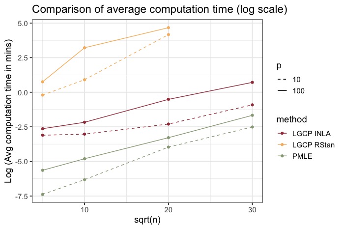
Figure 1: Average computation time for a single replicate of data in minutes, plotted on log scale, over 100 replicates for penalized PMLE and Bayesian LGCP model run via RStan and R-INLA.

Figure 2 compares our inference procedure with Bayesian inference, in terms of the coverage of confidence intervals, type I error rate and power. All three metrics are averaged across all relevant (e.g., non-zero for power) entries of ${\boldsymbol{\beta}}$. In low dimensions, Bayesian model fitted via INLA performs well, with power approaching 1 and well-controlled type I error rate along with valid $95\%$ coverage. Penalized PMLE achieves similar accuracy as well, but requires more samples. The reduced power is not surprising, given the over-parameterized nature of penalized PMLE, and the fact that it does not require or make use of the parametric distribution of $\varepsilon(\cdot)$. RStan fails to control the type I error and provide proper coverage, at least for the given amount of data and MCMC samples. With higher dimensions, Bayesian LGCP methods are not guaranteed to achieve the nominal $95\%$ coverage or control type I error within $0.05$, and we observe a trend of decreasing coverage for INLA as $m$ increases. In contrast, the penalized PMLE controls type I error rate within 0.05 and still maintains reasonable power despite being slightly conservative.

In the high-dimensional setting, the observation that INLA has good power and acceptable type I error rate but decreasing coverage could be explained by its non-decaying estimation bias for the non-zero parameters. Figure 3 visualizes the element-wise estimation errors for INLA and PMLE with different sample sizes ($n=10^{2}$ and $30^{2}$, respectively). The variability of estimation errors shrinks faster for INLA, reflecting higher efficiency due to its parametric nature. Estimates for the non-zero entries (index $1$ through 10) are attenuated for both methods, but this bias is decreasing for PMLE with more samples, while increasing for INLA. This issue occurs because the RW2D model for INLA assumes constant baseline risk on each observed cell, as well as a stationary error random field, both of which are violated in this simulation setting. Also, it is not clear how well INLA can handle high-dimensional covariates, as the current choice of priors on ${\boldsymbol{\beta}}$ does not induce shrinkage or regularization to handle high dimensionality. Shrinkage priors, such as horseshoe (Carvalho et al., 2009, 2010), may alleviate this issue but can be more computationally demanding.

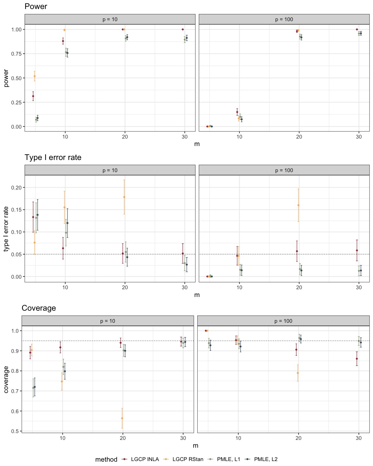
Figure 2: Comparison of coverage, type I error rate and power for penalized PMLE and Bayesian LGCP methods, with standard error bars.

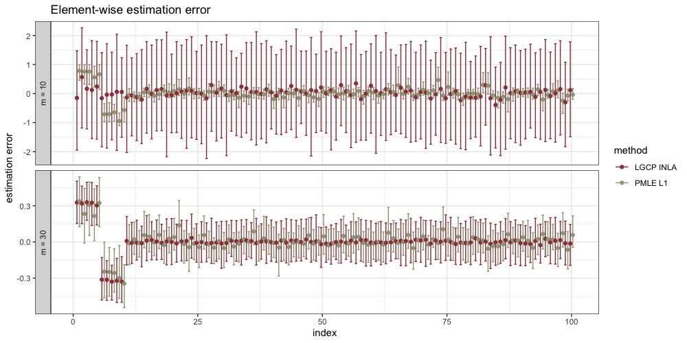
Figure 3: Average element-wise estimation errors along with the $5\%$ and $95\%$ percentiles of errors for $\beta$ in the high-dimensional ($p=100$) setting, with and $n=5^{2}$ (top) and $30^{2}$ (bottom) cells, respectively.

5 Application: Seattle Crime Data

We analyze the Seattle crime data to further demonstrate the performance of our approach in comparison with a wider range of alternative methods. We focus on crimes against persons that were reported to the Seattle Police Department in Spring 2021 (April 1 through June 30). Crime cases are recorded as point incidences (with blurred location) over the Seattle map, which we aggregate to the level of census tracts, since this is the finest resolution of covariates available. The population size of each census tract is used as offset. Covariates are obtained from King County GIS Open Data and include:

• Demographic and socioeconomic information: age distribution (proportion of residents in four age groups: 18-29, 30-44, 45-59, 60 and above); race/ethnicity distribution (proportion of Asian, Black, Hispanic, White populations, and populations with two or more races); median household income, education status (proportion of residents with college degree or above); and proportion of residents with medical insurance.

• Public facilities: number of hospitals; transit stops; fire stations; police stations; food facilities; schools; solid waste facilities; farmers’ markets;

• Environmental information: area of region; proportion of medium and high basins.

We purposely choose a wide range of covariates, including those that are not known as good predictors of crime rate. Covariates are all summarized by census tract. For covariates characterized by proportion of different groups (e.g. age, race/ethnicity, medium/high basins), we omit one category as the reference level and adopt the additive log ratio transformation (Aitchison, 1982) to alleviate the spurious correlation in such compositional data. The spatial domain is modeled as an unweighted graph, where two regions are connected if they share a common border.

We compare the penalized PMLE with $\ell_{1}$ and $\ell_{2}$ fusion penalties with the following Bayesian models, implemented in INLA. The default penalized complexity (PC) priors (Simpson et al., 2017) in the INLA R package are used for the variance, range (for LGCP) and mixing (for BYM2) parameters.

• The BYM2 model (Riebler et al., 2016) which specifies the linear predictor to be a sum of covariate effects, with spatially correlated errors induced by connectivity, and independent, non-spatial heterogeneity. The mixing parameter (which is between 0 and 1 and modeled on the logit scale) controls how much variance comes from the independent versus spatially dependent random effects.

• The LGCP model with independent Gaussian error random field.

• The LGCP model with Gaussian error random field having exponential covariance.

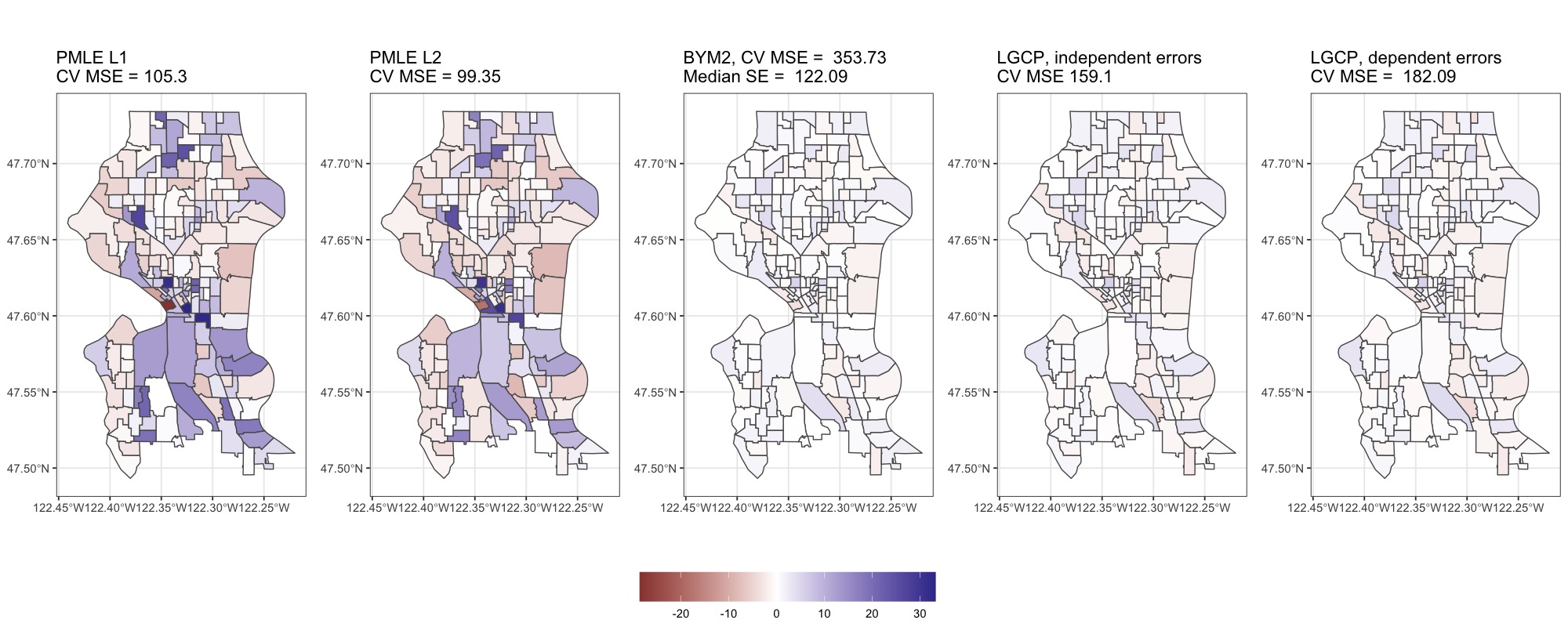
Figure 4: Residuals from each model, with cross-validated MSEs reported in the titles. Due to the large variability of prediction errors for the BYM2 model, we also report its median prediction SE for reference.

The predictive performance for each model is evaluated using 5-fold cross-validation. Figure 4 presents the residuals from each model along with their prediction MSEs. The residual plots capture how close each model fits to the data, while the prediction MSEs capture the overall predictive accuracy. The residual plots show that the Bayesian models have smaller bias comparing to penalized PMLE. However, the small bias comes at a cost of large variability, as reflected by the large MSE values and indicates over-fitting. Though LGCP with dependent errors conducts an implicit form of regularization for smoothness as achieved by a fusion penalty, such regularization is not explicit and it may thus be less straightforward to find a near-optimal bias and variance trade-off, compared to methods with explicit penalization.

Figure 5: Estimated rate ratios with error bars indicating $95\%$ confidence/credible intervals

Figure 5 presents point estimates along with $95\%$ confidence/credible intervals (CI/CrI) shown as error bars. The models all identify race and the number of food facilities to be associated with crime incidents within a region. The former matches other studies (Uehara, 1994; Krysan, 2008; Lodge et al., 2021) reporting challenges in the search of housing and/or housing inequalities associated with race, as well as residents of underrepresented race being exposed to higher crime rates. Lodge et al. (2021) also found such disparity by race and ethnicity to decrease when the granularity of data is not very high ($>$1600m buffer size, which is within the range of most census tracts in our case). This aligns with the reduced effect sizes of race and ethnicity estimated via PMLE compared to Bayesian models. PMLE leads to narrower CIs than Bayesian methods for this dataset in general. Also, when there is discrepancy in estimated effects reported by other models, PMLE tends to produce intermediate estimates. This can be seen, for example, for the effect of transit stops and schools. In addition, BYM2 finds medium basin, and both BYM2 and LGCP find the proportion of senior population to be positively associated with crime rates, which is somewhat hard to explain based on common knowledge. These findings align with our observation from Section 4 that PMLE could have a better control of type I error without significantly affecting its power.

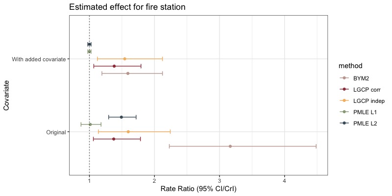
Figure 6: Comparison of estimated coefficients and $95\%$ CI/CrI before and after adding a spatially structured covariate to the single covariate model of fire station

A common concern in the analysis of spatial data is the effect of spatial confounding (Reich et al., 2006; Paciorek, 2010). The presence of spatial coufounding, which occurs when covariates contributing to the variability in the response are spatially structured, may introduce biases to the estimated effect sizes. To investigate how much the results of PMLE and the Bayesian models could be potentially impacted by this issue, we fit each model with fire station as the only covariate, and fit an additional set of models with a synthetic, spatially structured covariate added. Figure 6 compares the estimates along with 95% CI/CrI. We see that all models are not completely immune to spatial confounding, as indicated by the change in estimated effects after adding the spatially structured covariate; however, PMLE with $\ell_{1}$ fusion penalty and the two LGCP models are more robust against the inclusion of this spatially structured variable. As a sensitivity analysis for the choice of priors and computational approach, we also present and discuss an alternative version of Figures 5 and 6 in Appendix B where the Bayesian models are implemented via RStan with a different set of priors. We found that the model estimates and CrIs remain highly similar to Figure 5, while results from RStan are more sensitive to spatial confounding.

6 Discussion

We proposed a computationally simple approach to modeling semi-parametric, doubly-stochastic point processes with theoretical guarantees, focusing on the estimation and inference of fixed covariate effects. The key insight in the proposed method, which is based on a penalized regression framework, is that ignoring the stochasticity in the intensity and jointly modeling its realization along with the deterministic component still leads to a valid estimating function for the regression parameters. The nonparametric baseline is captured by a high-dimensional discretized intercept parameter. We solve this over-parametrized model with a fusion penalty for the region-specific intercepts, along with a sparsity penalty for the regression parameters. However, the soft constraint on smoothness does not need to hold exactly to ensure the validity of this penalization approach. We address the extra stochasticity in our statistical inference procedure and introduce robust covariance estimates under scenarios with and without stationarity of the error random field.

Literature on graph denoising may motivate further simplifications to the computational approach in the proposed Poisson maximum likelihood, or other graph-based spatial models. A sparse approximation to the edge incidence matrix $B_{n}$, as in Padilla et al. (2017), or an approximation to the graph Laplacian $L_{n}$, as in Sadhanala et al. (2016), could reduce the computational burden for large-scale settings. Establishing consistency and asymptotic normality in the the presence of such approximations would be an interesting topic of future research. Additional considerations may be helpful for selecting the threshold $\eta$ in the de-biasing procedure (see Equation 8) in practice, which controls the trade-off between type I error rate and power, especially with limited samples. Finaly, as noted in Section 2.3, prediction and parameter tuning may not be straightforward for graphical or spatial models, and naïve cross-validation is somewhat ad-hoc for correlated observations. Establishing theoretical guarantees for such an approach by leveraging recent developments in this area (Rabinowicz and Rosset, 2022) and/or incorporating alternative parameter tuning strategies that do not require sample splitting could be of interest.

APPENDIX

Appendix A Summary of Related Methods

Model	Method	Model Specification	Theoretical Guarantees
Cox process	Minimal contrast estimation (Diggle, 2003; Møller and Waagepetersen, 2003)	Parametric	N/A
	Bayesian estimation	Parametric	Convergence of LGCP posteriors under discretization (Waagepetersen, 2004)
	Bayesian estimation with INLA (Rue et al., 2009)	Parametric	N/A
	Bayesian estimation with variational approximation	Parametric	Convergence of posteriors to KL minimizer of a normal distribution (Wang and Blei, 2019)
	Bayesian estimation with basis function approximation of the random field (Simpson et al., 2016)	Random field with a basis expansion form	Convergence of basis function and discrete approximation, but not the full posterior
	Poisson maximum likelihood estimation (Schoenberg, 2005)	Known form for marginal means of the intensity	Consistency of parameters
	Composite likelihood estimation (Guan, 2006)	Stationarity or known form of second order intensity	Consistency and asymptotic normality of parameters
	Covariate-based kernel smoothing (Guan, 2008)	Nonparametric	Consistency
	Two-step estimation (Waagepetersen and Guan, 2009)	Known form of first- and second-order intensity functions	Consistency and asymptotic normality of parameters
Areal data model, e.g. Besag-York-Mollié (BYM) or BYM2 (Diggle, 2003; Møller and Waagepetersen, 2003; Riebler et al., 2016)	Bayesian estimation	Spatially correlated errors induced by connectivity, and independent non-spatial heterogeneity	N/A

Table 1: Comparison of existing models and estimation methods for doubly-stochastic spatial processes.

Appendix B Additional Results

Figures 7 and 8 present analogs of Figures 5 and 6, but with the BYM2 and LGCP models implemented in RStan based on two MCMC chains with 5000 samples each. All slope parameters are assigned Normal$(0,10)$ priors, and all variance parameters are assigned truncated Normal$(0,5)$ priors. We observe that the estimation and inference of the Bayesian models remain similar to the results shown in Figure 5, while LGCP models fitted by RStan are more sensitive to the inclusion of the spatially structured covariate (Figure 8), compared with INLA. In other words, the estimated the slope parameters are highly simlar between RStan and INLA, while the predicted spatial random effects from INLA appear to be more robust against spatial confounding. Such robustness is likely due to the properties of the PC priors (Simpson et al., 2017), along with the computational advantages of INLA.

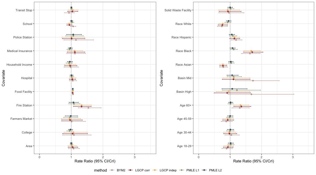
Figure 7: Estimated rate ratios with error bars indicating $95\%$ confidence/credible intervals from LGCP models fitted by RStan.

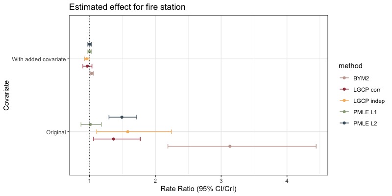
Figure 8: Comparison of estimated coefficients and $95\%$ CI/CrI before and after adding a spatially structured covariate to the single covariate model of fire station, with LGCP models fitted by RStan.

Appendix C Proofs

This section includes proofs for our theoretical claims in Section 3. We reintroduce our notation for clarity. The true, continuous baseline intensity is denoted as $\alpha^{0}(\cdot)$, and the true regression parameters are denoted as $\boldsymbol{\beta}^{0}$. We denote the discretized baseline vector, i.e. $\alpha^{0}(\cdot)$ evaluated at locations $\boldsymbol{s}=(s_{1},\ldots,s_{n})$, as ${\boldsymbol{\tilde{\alpha}}(\boldsymbol{s})}$ to distinguish it from the baseline intensity function. We also define $\phi(s)=\log\mathbb{E}_{0}[\exp\varepsilon(s)]$, $\boldsymbol{A}=(\lvert\Omega_{1}\rvert,\ldots,\lvert\Omega_{n}\rvert)$, $\boldsymbol{B}=(P_{1}\lvert\Omega_{1}\rvert,\ldots,P_{n}\lvert\Omega_{n}\rvert)$, and recall that $\ell(\cdot)$ is the Possion log-likelihood as defined in Section 2.

Empirical process notations are adopted, where under discretization of the observation window $\Omega$, we denote $\mathbb{P}_{0}f(\theta;X,Y):=\mathbb{E}_{0}[f(\theta;X,Y)]$ with $\mathbb{E}_{0}$ being the expectation taken under the true distribution of $X,Y$, and $\mathbb{P}_{n}f(\theta;X,Y):=n^{-1}\sum_{i}f(\theta;X_{i},Y_{i})$.

We first prove Lemma 1 by examining the relationship between the target parameter $\boldsymbol{\theta}^{\dagger}:=(\boldsymbol{\tilde{\alpha}}^{\dagger},\boldsymbol{\beta}^{\dagger})$, which is the solution to

$$-\nabla_{(\boldsymbol{\tilde{\alpha}},\boldsymbol{\beta})}\mathbb{P}_{0}\ell(\boldsymbol{\tilde{\alpha}},\boldsymbol{\beta})=0,$$

and the true parameter $\boldsymbol{\beta}^{0}$ along with the function $\alpha^{0}(\cdot)$ underlying the Cox process. In particular, we show that the Poisson likelihood yields an unbiased estimating equation for $\boldsymbol{\beta}$ despite the ignored error random field as well as misspecification of $\alpha^{0}(\cdot)$. With the fusion penalty $R(\boldsymbol{\tilde{\alpha}};\mathcal{G}_{n})$ incorporated into the objective function, we further bound the gap between the penalized solution $\boldsymbol{\theta}^{*}$ and $\boldsymbol{\theta}^{\dagger}$ under different conditions on the smoothness of $\alpha^{0}(\cdot)$.

We then use empirical process arguments to show the convergence of the penalized PMLE to the target parameters, following a similar outline as in Haris et al. (2019), with an adaptation to the heavy-tailed distribution of the observations in our setting due to double stochasticity.

Finally, we establish the asymptotic linearity of the de-biased estimator $\hat{\boldsymbol{b}}$ and in turn show the validity of our variance estimator along with the inference procedure.

C.1 Consistency

Throughout this section, we denote the smooth portion of our objective function as

$$\mathcal{L}(\boldsymbol{\theta}):=-\ell(\boldsymbol{\tilde{\alpha}},\boldsymbol{\beta})+\gamma_{n}R(\boldsymbol{\tilde{\alpha}};\mathcal{G}_{n}).$$

Also, without loss of generality, we assume a uniform offset $\boldsymbol{P}=(1,\ldots,1)^{\top}$ across all regions.

Proof of Lemma 1.

Note that for region $\Omega_{i},i\in\{1,\ldots,n\}$,

$$-\mathbb{P}_{0}\frac{\partial\ell}{\partial\tilde{\alpha}_{i}} =-\mathbb{E}_{X}\left[\mathbb{E}_{\varepsilon}\mathbb{E}[Y_{i}\mid\varepsilon(\cdot)]+{|\Omega_{i}|}\exp\left(\tilde{\alpha}_{i}+X_{i}\boldsymbol{\beta}\right)\right]$$

$$=-\mathbb{E}_{X}\left[\mathbb{E}_{\varepsilon}\int_{\Omega_{i}}\Lambda(s)\text{d}s+{|\Omega_{i}|}\exp\left(\tilde{\alpha}_{i}+X_{i}\boldsymbol{\beta}\right)\right]$$

$$=-\mathbb{E}_{X}\left[\int_{\Omega_{i}}\mathbb{E}_{\varepsilon}\exp\left[\alpha^{0}(s)+X_{i}\boldsymbol{\beta}^{0}+\varepsilon(s)\right]\text{d}s+{|\Omega_{i}|}\exp\left(\tilde{\alpha}_{i}+X_{i}\boldsymbol{\beta}\right)\right]$$ (11)

$$=-\mathbb{E}_{X}\left[\int_{\Omega_{i}}\exp\left[\alpha^{0}(s)+X_{i}\boldsymbol{\beta}^{0}+\phi(s)\right]\text{d}s+{|\Omega_{i}|}\exp\left(\tilde{\alpha}_{i}+X_{i}\boldsymbol{\beta}\right)\right],$$ (12)

where $\mathbb{E}_{\varepsilon}$ denotes expectation taken with respect to the error random field. “$=$” in (11) holds due to Fubini’s Theorem under Assumption 1. Furthermore, the mean value theorem for integrals together with Assumption 1 imply the existence of some $s_{i}^{*}\in\Omega_{i}$ such that

$$\int_{\Omega_{i}}\exp\left[\alpha^{0}(s)+X_{i}\boldsymbol{\beta}^{0}+\phi(s)\right]\text{d}s+{|\Omega_{i}|}\exp\left(\tilde{\alpha}_{i}+X_{i}\boldsymbol{\beta}\right)=-|\Omega_{i}|\exp\left[\alpha^{0}(s_{i}^{*})+X_{i}\boldsymbol{\beta}^{0}+\phi(s_{i}^{*})\right]+{|\Omega_{i}|}\exp\left(\tilde{\alpha}_{i}+X_{i}\boldsymbol{\beta}\right)$$ (13)

for any realization of $X$. We write $\boldsymbol{s}^{*}=(s_{1}^{*},\ldots,s_{n}^{*})$ such that $s_{i}^{*}\in\Omega_{i}$ for all $i$. Define the target parameter $\boldsymbol{\theta}^{\dagger}=(\boldsymbol{\alpha}^{\dagger},\boldsymbol{\beta}^{\dagger})$ such that $\boldsymbol{\alpha}^{\dagger}=\alpha^{0}(\boldsymbol{s}^{*})+\phi(\boldsymbol{s}^{*})$ and $\boldsymbol{\beta}^{\dagger}=\boldsymbol{\beta}^{0}$. Examining the expression in (13) leads to

$$-\frac{\partial}{\partial\tilde{\alpha}_{i}}\mathbb{P}_{0}\ell(\tilde{\boldsymbol{\alpha}},\boldsymbol{\beta})\big{|}_{{\boldsymbol{\alpha}^{\dagger}},\boldsymbol{\beta}^{\dagger}}=0.$$

Likewise, since

$$-\nabla_{\boldsymbol{\beta}}\mathbb{E}_{0}[\ell(\tilde{\boldsymbol{\alpha}},\boldsymbol{\beta})\mid X]=-\sum_{i=1}^{n}X_{i}\frac{\partial}{\partial\tilde{\alpha}_{i}}\mathbb{E}_{0}[\ell(\tilde{\boldsymbol{\alpha}},\boldsymbol{\beta})\mid X],$$

we also have

$$-\nabla_{\boldsymbol{\beta}}\mathbb{P}_{0}\ell(\tilde{\boldsymbol{\alpha}},\boldsymbol{\beta})\big{|}_{{\boldsymbol{\alpha}^{\dagger}},\boldsymbol{\beta}^{\dagger}}=0.$$

Together with the convexity of $-\ell(\cdot)$, we established the form of target parameter $\boldsymbol{\theta}^{\dagger}$ as claimed in Lemma 1.

We now examine the minimizer $\boldsymbol{\theta}^{*}$ of $\mathcal{L}(\cdot)$. First, observe that $\mathcal{L}(\boldsymbol{\theta})$ involves $\boldsymbol{\beta}$ only through $-\ell(\boldsymbol{\theta})$, we immediately have $\nabla_{\boldsymbol{\beta}}\mathcal{L}(\boldsymbol{\alpha}^{*},\boldsymbol{\beta}^{\dagger})=0$ which yields $\boldsymbol{\beta}^{*}=\boldsymbol{\beta}^{\dagger}=\boldsymbol{\beta}^{0}$ again by the convexity of $-\ell(\cdot)$.

We first discuss the case with $\ell_{2}$ smoothing penalty. By the optimality of $\boldsymbol{\theta}^{*}$ and conducting a Taylor expansion of $\mathcal{L}$ around $\boldsymbol{\theta}^{\dagger}$, we have

$$0 =-\nabla_{\boldsymbol{\tilde{\alpha}}}[\mathbb{P}_{0}\ell(\boldsymbol{\alpha}^{*},\boldsymbol{\beta}^{*})+\gamma_{n}R(\boldsymbol{\alpha}^{*})]$$

$$=-\mathbb{E}_{0}\left[\boldsymbol{Y}-A\odot\exp(\boldsymbol{\alpha}^{*}+\boldsymbol{X}\boldsymbol{\beta}^{*})\right]+\gamma_{n}\nabla_{\tilde{\boldsymbol{\alpha}}}R(\boldsymbol{\alpha}^{*})$$ (14)

$$=-\mathbb{E}_{0}\left[\boldsymbol{Y}-A\odot\exp(\boldsymbol{\alpha}^{\dagger}+\boldsymbol{X}\boldsymbol{\beta}^{\dagger})\right]+\gamma_{n}\nabla_{\tilde{\boldsymbol{\alpha}}}R(\boldsymbol{\alpha}^{\dagger})+\left[\text{diag}\left(A\odot\exp(\breve{\boldsymbol{\alpha}}+\boldsymbol{X}\boldsymbol{\beta}^{\dagger})\right)+\gamma_{n}\nabla_{\tilde{\boldsymbol{\alpha}}}^{2}R(\breve{\boldsymbol{\alpha}})\right]\left(\boldsymbol{\alpha}^{*}-\boldsymbol{\alpha}^{\dagger}\right)$$

for some $\breve{\boldsymbol{\alpha}}$ between $\boldsymbol{\alpha}^{*}$ and $\boldsymbol{\alpha}^{\dagger}$, where $\odot$ denotes element-wise multiplication. Since $-\mathbb{E}_{0}\left[\boldsymbol{Y}-A\odot\exp(\boldsymbol{\alpha}^{\dagger}+\boldsymbol{X}\boldsymbol{\beta}^{\dagger})\right]=0$, we then have

$$\boldsymbol{\alpha}^{*}-\boldsymbol{\alpha}^{\dagger}=\left[\text{diag}\left(A\odot\exp(\breve{\boldsymbol{\alpha}}+\boldsymbol{X}\boldsymbol{\beta}^{\dagger})\right)+\gamma_{n}\nabla_{\tilde{\boldsymbol{\alpha}}}^{2}R(\breve{\boldsymbol{\alpha}})\right]^{-1}\left[\gamma_{n}\nabla_{\tilde{\boldsymbol{\alpha}}}R(\boldsymbol{\alpha}^{\dagger})\right]$$

and

$$\lVert\boldsymbol{\alpha}^{*}-\boldsymbol{\alpha}^{\dagger}\rVert_{2} \leq\gamma_{n}\left\lVert\left[\text{diag}\left(A\odot\exp(\breve{\boldsymbol{\alpha}}+\boldsymbol{X}\boldsymbol{\beta}^{\dagger})\right)+\gamma_{n}\nabla^{2}_{\tilde{\boldsymbol{\alpha}}}R(\breve{\boldsymbol{\alpha}})\right]^{-1}\right\rVert_{2}\lVert\nabla_{\tilde{\boldsymbol{\alpha}}}R(\boldsymbol{\alpha}^{\dagger})\rVert_{2}$$

$$\leq\gamma_{n}\lambda_{\min}\left[\text{diag}\left(A\odot\exp(\breve{\boldsymbol{\alpha}}+\boldsymbol{X}\boldsymbol{\beta}^{\dagger})\right)+\gamma_{n}(L_{n}+\delta I_{n})\right]^{-1}\frac{1}{2}\lVert(L_{n}+\delta I_{n})\boldsymbol{\alpha}^{\dagger}\rVert_{2}$$

$$\leq\frac{\gamma_{n}}{2}\lVert\tilde{L}_{n}\boldsymbol{\alpha}^{\dagger}(\boldsymbol{s}^{*})\rVert_{2}\left[\max_{i}A_{i}\exp(\breve{\boldsymbol{\alpha}_{i}}+X_{i}\boldsymbol{\beta}^{\dagger})\right]^{-1}$$

$$=\gamma_{n}\lVert\tilde{L}_{n}\boldsymbol{\alpha}^{\dagger}(\boldsymbol{s}^{*})\rVert_{2}\cdot O_{P}(1)$$

where $\lambda_{\min}(\cdot)$ denotes the smallest eigenvalue of a matrix. We have made use of the boundedness of $\max_{i}|\Omega_{i}|$, the continuity of $\alpha(\cdot)$, and the fact that $L_{n}+\delta I_{n}$ is positive semi-definite. It then follows directly that $\lVert\boldsymbol{\alpha}^{*}-\boldsymbol{\alpha}^{\dagger}\rVert_{2}$ is $O_{P}(n^{c})$ under Assumption 2 i-ii), and $o_{P}(1)$ if Assumption 2 iii) further holds.

For the $\ell_{1}$ fusion penalty, recall that the gradient of the smoothed penalty is $\nabla_{\boldsymbol{\tilde{\alpha}}}R(\tilde{\boldsymbol{\alpha}})=B_{n}^{\top}S_{\infty}(\gamma_{n}B_{n}\tilde{\boldsymbol{\alpha}}/\xi)$ and that $S_{\infty}(\cdot)$ represents projection onto the $\ell_{\infty}$ unit ball. Continuing from (14) with a Taylor expansion of $\ell(\tilde{\boldsymbol{\alpha}},\boldsymbol{\beta})$ with respect to $\tilde{\boldsymbol{\alpha}}$,

$$0 =-\mathbb{E}_{0}\left[\boldsymbol{Y}-A\odot\exp(\boldsymbol{\alpha}^{*}+\boldsymbol{X}\boldsymbol{\beta}^{*})\right]+\gamma_{n}\nabla_{\tilde{\boldsymbol{\alpha}}}R(\boldsymbol{\alpha}^{*})$$

$$=-\mathbb{E}_{0}\left[\boldsymbol{Y}-A\odot\exp(\boldsymbol{\alpha}^{\dagger}+\boldsymbol{X}\boldsymbol{\beta}^{\dagger})\right]+\gamma_{n}\nabla_{\tilde{\boldsymbol{\alpha}}}R(\boldsymbol{\alpha}^{*})+\left[\text{diag}\left(A\odot\exp(\breve{\boldsymbol{\alpha}}+\boldsymbol{X}\boldsymbol{\beta}^{\dagger})\right)\right]\left(\boldsymbol{\alpha}^{*}-\boldsymbol{\alpha}^{\dagger}\right)$$

$$=-\mathbb{E}_{0}\left[\boldsymbol{Y}-A\odot\exp(\boldsymbol{\alpha}^{\dagger}+\boldsymbol{X}\boldsymbol{\beta}^{\dagger})\right]+\gamma_{n}\nabla_{\tilde{\boldsymbol{\alpha}}}R(\boldsymbol{\alpha}^{\dagger})+\left[\text{diag}\left(A\odot\exp(\breve{\boldsymbol{\alpha}}+\boldsymbol{X}\boldsymbol{\beta}^{\dagger})\right)\right]\left(\boldsymbol{\alpha}^{*}-\boldsymbol{\alpha}^{\dagger}\right)+\gamma_{n}\left[\nabla_{\boldsymbol{\tilde{\alpha}}}R({\boldsymbol{\alpha}}^{*})-\nabla_{\boldsymbol{\tilde{\alpha}}}R({\boldsymbol{\alpha}}^{\dagger})\right]$$

which leads to

$$\lVert\boldsymbol{\alpha}^{*}-\boldsymbol{\alpha}^{\dagger}\rVert_{1} \leq\gamma_{n}\left[\max_{i}A_{i}\exp(\breve{\boldsymbol{\alpha}_{i}}+X_{i}\boldsymbol{\beta}^{\dagger})\right]^{-1}\bigg{[}\left\lVert\nabla_{\tilde{\boldsymbol{\alpha}}}R(\boldsymbol{\alpha}^{\dagger})\right\rVert_{1}+\left\lVert\nabla_{\boldsymbol{\tilde{\alpha}}}R({\boldsymbol{\alpha}}^{*})-\nabla_{\boldsymbol{\tilde{\alpha}}}R({\boldsymbol{\alpha}}^{\dagger})\right\rVert_{1}\bigg{]}$$

$$\leq\gamma_{n}\left[\max_{i}A_{i}\exp(\breve{\boldsymbol{\alpha}_{i}}+X_{i}\boldsymbol{\beta}^{\dagger})\right]^{-1}\bigg{[}\left\lVert B_{n}^{\top}S_{\infty}\left(\frac{\gamma_{n}B_{n}{\boldsymbol{\alpha}}^{\dagger}}{\xi}\right)\right\rVert_{1}+\left\lVert B_{n}^{\top}\left(S_{\infty}\left(\frac{\gamma_{n}B_{n}{\boldsymbol{\alpha}}^{*}}{\xi}\right)-S_{\infty}\left(\frac{\gamma_{n}B_{n}{\boldsymbol{\alpha}}^{\dagger}}{\xi}\right)\right)\right\rVert_{1}\bigg{]}$$

$$\leq\gamma_{n}O_{P}(1)\left[\frac{\gamma_{n}}{\xi}\lVert B_{n}^{\top}\rVert_{1}\lVert B_{n}{\boldsymbol{\alpha}}^{\dagger}\rVert_{1}+\frac{\gamma_{n}}{\xi}\lVert B_{n}^{\top}\rVert_{1}\lVert B_{n}\rVert_{1}\lVert{\boldsymbol{\alpha}}^{*}-{\boldsymbol{\alpha}}^{\dagger}\rVert_{1}\right]$$ (15)

where (15) holds because $\lVert S_{\infty}(u)\rVert_{1}\leq\lVert u\rVert_{1}$ and $\lVert S_{\infty}(u)-S_{\infty}(v)\rVert_{1}\leq\lVert u-v\rVert_{1}$ for any vectors $u$ and $v$. Noting that $\lVert B_{n}^{\top}\rVert_{1}=2$ (which is the maximum row sum of absolute values of $B_{n}$) and $\lVert B_{n}\rVert_{1}=\max_{i}d_{i}$ (which is the maximum column sum of absolute values of $B_{n}$), when $n$ is large so that $\gamma_{n}^{2}\max_{i}d_{i}<\xi/2$, (15) yields

$$\frac{1}{2}\lVert{\boldsymbol{\alpha}}^{*}-{\boldsymbol{\alpha}}^{\dagger}\rVert_{1}\leq\frac{\gamma_{n}^{2}}{\xi}O_{P}(1)\lVert B_{n}{\boldsymbol{\alpha}}^{\dagger}\rVert_{1}.$$

Consequently, we also have for the $\ell_{1}$ fusion penalty that $\lVert{\boldsymbol{\alpha}}^{*}-{\boldsymbol{\alpha}}^{\dagger}\rVert_{1}$ is $O_{P}(n^{c})$ under Assumption 2 i-ii), and $o_{P}(1)$ if Assumption 2 iii) further holds. ∎

Proof of Theorem 1.

Our estimator is given by $\hat{\boldsymbol{\theta}}=\operatornamewithlimits{argmin}_{\boldsymbol{\theta}}\mathbb{P}_{n}\mathcal{L}(\boldsymbol{\theta})+\tau_{n}\lVert\boldsymbol{\beta}\rVert_{1}$. We denote the marginal mean $\boldsymbol{\mu}=(\mu_{1},\ldots,\mu_{n})$ as $\mu_{i}:=\mathbb{E}_{\varepsilon}\int_{\Omega_{i}}\exp[\alpha(s)+X_{i}\boldsymbol{\beta}+\varepsilon(s)]\text{d}s$. Define the empirical process term

$$\nu_{n}(\boldsymbol{\theta})=(\mathbb{P}_{n}-\mathbb{P})\mathcal{L}(\boldsymbol{\theta})$$

and the excess risk

$$\mathcal{E}(\boldsymbol{\theta})=\mathbb{P}(\mathcal{L}(\boldsymbol{\theta})-\mathcal{L}(\boldsymbol{\theta}^{*})).$$

Similar to the logic of Haris et al. (2019), we examine

$$\nu_{n}(\boldsymbol{\theta})-\nu_{n}(\boldsymbol{\theta}^{*}) =\frac{1}{n}\sum_{i=1}^{n}(Y_{i}-\mu_{i})\left[(\alpha_{i}-\alpha_{i}^{*})+\sum_{j=1}^{p}\left(\beta_{j}x_{ij}-\beta^{*}_{j}x_{ij}\right)\right]$$

$$=\frac{1}{n}\sum_{i=1}^{n}(Y_{i}-\mu_{i})(\alpha_{i}-\alpha_{i}^{*})+\frac{1}{n}\sum_{i=1}^{n}\sum_{j=1}^{p}(Y_{i}-\mu_{i})(\beta_{j}x_{ij}-\beta^{*}_{j}x_{ij}):=\text{I}+\text{II},$$ (16)

and analyze the two terms separately. First, define $a_{i}=\frac{\alpha_{i}-\alpha_{i}^{*}}{\lVert\boldsymbol{\alpha}-\boldsymbol{\alpha}^{*}\rVert_{1}}$; then for any $\rho>0$, term I satisfies

$$\Pr\left(\left\lvert\frac{\sum_{i}(Y_{i}-\mu_{i})(\alpha_{i}-\alpha_{i}^{*})}{n\lVert\boldsymbol{\alpha}-\boldsymbol{\alpha}^{*}\rVert_{1}}\right\rvert>\rho\right)\leq\frac{\mathbb{E}_{0}|\sum_{i}a_{i}(Y_{i}-\mu_{i})|^{2}}{\rho^{2}n^{2}}\leq\frac{2\sum_{i}a_{i}^{2}\text{Var}(Y_{i})}{\rho^{2}n^{2}}\leq\frac{2(\sum_{i}a_{i}^{2})\max_{i}\text{Var}(Y_{i})}{\rho^{2}n^{2}}$$ (17)

where the first “$\leq$” holds by Chebyshev’s inequality. Furthermore, by the law of total variance, we have

$$\text{Var}(Y_{i})=\mathbb{E}_{\varepsilon}\text{Var}(Y_{i}\mid\varepsilon)+\text{Var}_{\varepsilon}\mathbb{E}[Y_{i}\mid\varepsilon]=\mathbb{E}_{0}\mu_{i}+\mathbb{E}_{0}\mu_{i}^{2},$$

which satisfies

$$\mathbb{E}_{0}\mu_{i}^{k} =\mathbb{E}_{0}\int_{\Omega_{i}}\exp\left[k(\alpha(s)+X_{i}\boldsymbol{\beta}+\varepsilon(s))\right]\text{d}s$$

$$=\mathbb{\int}_{\Omega_{i}}\exp\left[k(\alpha(s)+X_{i}\boldsymbol{\beta}]\mathbb{E}_{0}\exp[k\varepsilon(s)]\right]\text{d}s$$

where $k=1,2$. By Assumption 4 along with the fact that $|\Omega_{i}|$ is bounded, we have $\max_{i}\mathbb{E}_{0}\mu_{i}^{k}<$ (some) $M<\infty$. Furthermore, it holds that $\sum_{i}a_{i}^{2}=\lVert\boldsymbol{\alpha}-\boldsymbol{\alpha}^{*}\rVert_{2}^{2}/\lVert\boldsymbol{\alpha}-\boldsymbol{\alpha}^{*}\rVert_{1}^{2}\leq 1$ by construction.

Returning to (17), we now established

$$\Pr\left(\left\lvert\frac{\sum_{i}(Y_{i}-\mu_{i})(\alpha_{i}-\alpha_{i}^{*})}{n\lVert\boldsymbol{\alpha}-\boldsymbol{\alpha}^{*}\rVert_{1}}\right\rvert>\rho\right)\leq C_{\alpha,\beta,\varepsilon}(n\rho)^{-2}$$ (18)

for some constant $C_{\alpha,\beta,\varepsilon}$. Likewise, for term II, let

$$b_{ij}=\frac{\beta_{j}x_{ij}-\beta^{*}_{j}x_{ij}}{n|\beta_{j}-\beta^{*}_{j}|}.$$

It then follows that

$$\lVert b_{\cdot j}\rVert_{2}^{2}=\frac{\sum_{i}x_{ij}^{2}}{n^{2}}\leq\frac{R^{2}}{n},$$

and

$$\lVert b_{\cdot j}\rVert_{\infty}\leq\frac{R}{n}$$

by Assumption 6. Therefore, by a similar argument as for term I, for any $\rho>0$,

$$\Pr\left(\left\lvert\frac{\sum_{i}(Y_{i}-\mu_{i})(\beta_{j}x_{ij}-\beta^{*}_{i}x_{ij})}{n|\beta_{j}-\beta_{j}^{*}|}\right\rvert>\rho\right)\leq\frac{|\sum_{i}b_{ij}\text{Var}(Y_{i})|}{\rho^{2}n^{2}}\leq\frac{2\sum b_{ij}^{2}\text{Var}(Y_{i})}{\rho^{2}n^{2}}\leq C_{\alpha,\beta,\varepsilon}R^{2}n^{-3}\rho^{-2}.$$

Applying a union bound yields

$$\Pr\left(\max_{j\in[p]}\left\lvert\frac{\sum_{i}(Y_{i}-\mu_{i})(\beta_{j}x_{ij}-\beta^{*}_{i}x_{ij})}{n|\beta_{j}-\beta_{j}^{*}|}\right\rvert>\rho\right)\leq C_{\alpha,\beta,\varepsilon}R^{2}(n\rho)^{-2}.$$ (19)

Plugging into (16) yields that with probability $\geq 1-C_{1}(n\rho)^{-2}$ for some constant $C_{1}$,

$$|\nu_{n}(\boldsymbol{\theta})-\nu_{n}(\boldsymbol{\theta}^{*})|\leq\rho\left[\lVert\boldsymbol{\alpha}-\boldsymbol{\alpha}^{*}\rVert_{1}+\lVert\boldsymbol{\beta}-\boldsymbol{\beta}^{*}\rVert_{1}\right].$$ (20)

Next, note that

$$\lambda_{\min}\left[\nabla^{2}_{\boldsymbol{\theta}}\mathcal{L}\right]\geq\lambda_{\min}\left\{\begin{bmatrix}I_{n}\\ \boldsymbol{X}^{\top}\end{bmatrix}\boldsymbol{D}\begin{bmatrix}I_{n}&\boldsymbol{X}\end{bmatrix}\right\}$$

where $\boldsymbol{D}=diag(\exp(\alpha_{i}+X_{i}\boldsymbol{\beta}))$. Note also that the eigenvalues of $\nabla^{2}_{\boldsymbol{\theta}}\mathcal{L}$ are determined by those of $\boldsymbol{D}$ and $\boldsymbol{X}^{\top}\boldsymbol{D}\boldsymbol{X}$, the restricted eigenvalue condition in Assumption 6 along with the (lower-)bounded intensity condition in Assumption 4 guarantee that

$$\lambda_{\min}\left[\nabla^{2}_{\boldsymbol{\theta}}\mathcal{L}\right]\geq(some)\ m>0$$

for all $\boldsymbol{\theta}\in\mathcal{B}$ as defined in Assumption 6 (we recall $\mathcal{B}=\{\theta:\lVert\theta-\theta^{*}\rVert_{1}\leq 4\tau_{n}^{2}s/c\rho\varphi_{s}^{2}\}$), establishing the restricted strong convexity of $\mathcal{L}$.

For convenience, let $M^{*}=\frac{4\tau_{n}^{2}s}{c\rho\varphi_{s}^{2}}$. Define

$$Z_{M^{*}}:=\sup_{\boldsymbol{\theta}\in\mathcal{B}}|\nu_{n}(\theta)-\nu_{n}(\theta^{*})|.$$

We have just shown that

$$Z_{M^{*}}\leq\rho\left[\lVert\boldsymbol{\alpha}-\boldsymbol{\alpha}^{*}\rVert_{1}+\lVert\boldsymbol{\beta}-\boldsymbol{\beta}^{*}\rVert_{1}\right]\leq\rho M^{*}$$

with probability $\geq 1-C_{1}(n\rho)^{-2}$.

Similar to the approach of Haris et al. (2019), set

$$t=\frac{M^{*}}{M^{*}+\lVert\hat{\boldsymbol{\alpha}}-\boldsymbol{\alpha}^{*}\rVert_{1}+\lVert\hat{\boldsymbol{\beta}}-\boldsymbol{\beta}^{*}\rVert_{1}}$$

and let $\breve{\boldsymbol{\theta}}=t\hat{\boldsymbol{\theta}}+(1-t)\boldsymbol{\theta}^{*}$. Then

$$\lVert\breve{\boldsymbol{\theta}}-\boldsymbol{\theta}^{*}\rVert_{1}=t\lVert\hat{\boldsymbol{\theta}}\rVert_{1}\leq\frac{M^{*}}{\lVert\hat{\boldsymbol{\alpha}}-\boldsymbol{\alpha}^{*}\rVert_{1}+\lVert\hat{\boldsymbol{\beta}}-\boldsymbol{\beta}^{*}\rVert_{1}}\lVert\hat{\boldsymbol{\theta}}\rVert_{1}=M^{*}$$

so that $\breve{\boldsymbol{\theta}}\in\mathcal{B}$. By the basic inequalities due to the optimality of $\hat{\boldsymbol{\theta}}$ and the convexity of $\mathcal{L}$,

$$\mathcal{E}(\hat{\boldsymbol{\theta}})+\tau_{n}\lVert\hat{\boldsymbol{\theta}}\rVert_{1} \leq-[\nu_{n}(\hat{\boldsymbol{\theta}})-\nu_{n}(\boldsymbol{\theta}^{*})]+\tau_{n}\lVert{\boldsymbol{\theta}}^{*}\rVert_{1},$$

$$\mathcal{E}(\breve{\boldsymbol{\theta}})+\tau_{n}\lVert\breve{\boldsymbol{\theta}}\rVert_{1} \leq-[\nu_{n}(\breve{\boldsymbol{\theta}})-\nu_{n}(\boldsymbol{\theta}^{*})]+\tau_{n}\lVert{\boldsymbol{\theta}}^{*}\rVert_{1}\leq Z_{M^{*}}+\lambda\lVert\boldsymbol{\theta}^{*}\rVert_{1}\leq\rho M^{*}+\lambda\lVert\boldsymbol{\theta}^{*}\rVert_{1}.$$ (21)

Further by the separability of $\lVert\cdot\rVert_{1}$, we have

$$\tau_{n}\lVert{\boldsymbol{\beta}}^{*}\rVert_{1}\leq\tau_{n}[\lVert{\boldsymbol{\beta}}^{*}_{S}-\breve{\boldsymbol{\beta}}_{S}\rVert_{1}+\lVert\breve{\boldsymbol{\beta}}_{S}\rVert_{1}],$$

and

$$\tau_{n}\lVert\breve{\boldsymbol{\beta}}\rVert_{1}=\tau_{n}[\lVert\breve{\boldsymbol{\beta}}_{S}\rVert_{1}+\lVert(\breve{\boldsymbol{\beta}}-{\boldsymbol{\beta}}^{*})_{S^{C}}\rVert_{1}]$$

due to the sparsity of $\boldsymbol{\beta}^{*}$. Plugging into (21), we obtain

$$\mathcal{E}(\breve{\boldsymbol{\theta}})+\tau_{n}\left[\lVert\breve{\boldsymbol{\beta}}_{S}\rVert_{1}+\lVert(\breve{\boldsymbol{\beta}}-{\boldsymbol{\beta}}^{*})_{S^{C}}\rVert_{1}\right]\leq\rho M^{*}+\tau_{n}\left[\lVert{\boldsymbol{\beta}}^{*}_{S}-\breve{\boldsymbol{\beta}}_{S}\rVert_{1}+\lVert\breve{\boldsymbol{\beta}}_{S}\rVert_{1}\right].$$

Adding $\tau_{n}\left[\lVert\breve{\boldsymbol{\alpha}}-{\boldsymbol{\alpha}}^{*}\rVert_{1}+\lVert(\breve{\boldsymbol{\beta}}-{\boldsymbol{\beta}}^{*})_{S}\rVert_{1}\right]$ to both sides,

$$\mathcal{E}(\breve{\boldsymbol{\theta}})+\tau_{n}\left[\lVert\breve{\boldsymbol{\alpha}}-{\boldsymbol{\alpha}}^{*}\rVert_{1}+\lVert\breve{\boldsymbol{\beta}}-{\boldsymbol{\beta}}^{*}\rVert_{1}\right]\leq\rho M^{*}+\tau_{n}\lVert\breve{\boldsymbol{\alpha}}-{\boldsymbol{\alpha}}^{*}\rVert_{1}+2\tau_{n}\lVert(\breve{\boldsymbol{\beta}}-{\boldsymbol{\beta}}^{*})_{S}\rVert_{1}.$$ (22)

From here we consider two scenarios for (22). In both cases, we set $\rho=O(\sqrt{(\log p)/n})$ and $\tau_{n}\asymp\rho$ such that $\tau_{n}\geq 8\rho$. When $\rho M^{*}\leq\tau_{n}\lVert\breve{\boldsymbol{\alpha}}-{\boldsymbol{\alpha}}^{*}\rVert_{1}+2\tau_{n}\lVert(\breve{\boldsymbol{\beta}}-{\boldsymbol{\beta}}^{*})_{S}\rVert_{1}$, (22) becomes

$$\mathcal{E}(\breve{\boldsymbol{\theta}})+\tau_{n}\lVert(\breve{\boldsymbol{\beta}}-{\boldsymbol{\beta}}^{*})_{S^{C}}\rVert_{1}\leq\tau_{n}\lVert\breve{\boldsymbol{\alpha}}-{\boldsymbol{\alpha}}^{*}\rVert_{1}+3\tau_{n}\lVert(\breve{\boldsymbol{\beta}}-{\boldsymbol{\beta}}^{*})_{S}\rVert_{1}$$

$$\Rightarrow \lVert(\breve{\boldsymbol{\beta}}-{\boldsymbol{\beta}}^{*})_{S^{C}}\rVert_{1}\leq\lVert\breve{\boldsymbol{\alpha}}-{\boldsymbol{\alpha}}^{*}\rVert_{1}+3\lVert(\breve{\boldsymbol{\beta}}-{\boldsymbol{\beta}}^{*})_{S}\rVert_{1}.$$

Comparing with Assumption 3, we see that $\breve{\boldsymbol{\beta}}-{\boldsymbol{\beta}}^{*}\in\mathcal{C}(S)$. Under the compatibility condition,

$$\mathcal{E}(\breve{\boldsymbol{\theta}})+\tau_{n}\left[\lVert\breve{\boldsymbol{\alpha}}-{\boldsymbol{\alpha}}^{*}\rVert_{1}+\lVert\breve{\boldsymbol{\beta}}-{\boldsymbol{\beta}}^{*}\rVert_{1}\right] \leq\frac{4\tau_{n}\lVert\breve{\boldsymbol{\theta}}-\boldsymbol{\theta}^{*}\rVert_{2}\sqrt{s}}{\varphi_{s}}$$

$$\leq\frac{16\tau_{n}^{2}s}{4c\varphi_{s}^{2}}+c\lVert\breve{\boldsymbol{\theta}}-\boldsymbol{\theta}^{*}\rVert_{2}^{2}\text{ for }c=\frac{4\tau_{n}\sqrt{s}}{\varphi_{s}}$$

$$\leq\frac{4\tau_{n}^{2}s}{c\varphi_{s}^{2}}+\mathcal{E}(\breve{\boldsymbol{\theta}})$$ (23)

where the second line follows from a convex conjugate argument, namely, letting $H(v)=\sup_{u}\{uv-cu^{2}\}$ for $v\geq 0$ and some constant $c$, then $H(v)=v^{2}/4c$. The third line is implied by the restricted strong convexity of $\mathcal{L}$ since $\breve{\boldsymbol{\theta}}\in\mathcal{B}$.

Continuing from (23),

$$\mathcal{E}(\breve{\boldsymbol{\theta}})+\tau_{n}\left[\lVert\breve{\boldsymbol{\alpha}}-{\boldsymbol{\alpha}}^{*}\rVert_{1}+\lVert\breve{\boldsymbol{\beta}}-{\boldsymbol{\beta}}^{*}\rVert_{1}\right]\leq\rho M^{*}+\mathcal{E}(\breve{\boldsymbol{\theta}})\leq\frac{\tau_{n}M^{*}}{8}+\mathcal{E}(\breve{\boldsymbol{\theta}}),$$ (24)

leading to $\lVert\breve{\boldsymbol{\theta}}-\boldsymbol{\theta}^{*}\rVert_{1}\leq M^{*}/8$. Then, by construction of $t$,

$$\lVert\hat{\boldsymbol{\theta}}-\boldsymbol{\theta}^{*}\rVert_{1} =\frac{1}{t}[\lVert\breve{\boldsymbol{\theta}}-\boldsymbol{\theta}^{*}\rVert_{1}]$$

$$\leq\left[1+\frac{\lVert\hat{\boldsymbol{\alpha}}-{\boldsymbol{\alpha}}^{*}\rVert_{1}+\lVert\hat{\boldsymbol{\beta}}-{\boldsymbol{\beta}}^{*}\rVert_{1}}{M^{*}}\right]\frac{M^{*}}{8}\leq\frac{1}{8}[M^{*}+\lVert\hat{\boldsymbol{\theta}}-\boldsymbol{\theta}^{*}\rVert_{1}].$$

we thus have $\lVert\hat{\boldsymbol{\theta}}-\boldsymbol{\theta}^{*}\rVert_{1}\leq M^{*}$ so that $\hat{\boldsymbol{\theta}}\in\mathcal{B}$ as well.

We then return to (22) to examine the second scenario where $\rho M^{*}>\tau_{n}\lVert\breve{\boldsymbol{\alpha}}-{\boldsymbol{\alpha}}^{*}\rVert_{1}+2\tau_{n}\lVert(\breve{\boldsymbol{\beta}}-{\boldsymbol{\beta}}^{*})_{S}\rVert_{1}$. In this case, (22) simply becomes

$$\mathcal{E}(\breve{\boldsymbol{\theta}})+\tau_{n}\left[\lVert\breve{\boldsymbol{\alpha}}-{\boldsymbol{\alpha}}^{*}\rVert_{1}+\lVert\breve{\boldsymbol{\beta}}-{\boldsymbol{\beta}}^{*}\rVert_{1}\right]\leq 2\rho M^{*}\leq\frac{\tau_{n}M^{*}}{4}$$

which leads to $\lVert\breve{\boldsymbol{\theta}}-\boldsymbol{\theta}^{*}\rVert_{1}\leq M^{*}/4$. Similar to the first scenario, we obtain $\lVert\hat{\boldsymbol{\theta}}-\boldsymbol{\theta}^{*}\rVert_{1}\leq M^{*}$ so that $\hat{\boldsymbol{\theta}}\in\mathcal{B}$. Namely,

$$\lVert\hat{\boldsymbol{\alpha}}-{\boldsymbol{\alpha}}^{*}\rVert_{1}+\lVert\hat{\boldsymbol{\beta}}-{\boldsymbol{\beta}}^{*}\rVert_{1}\leq M^{*}.$$

holds from (22) in both cases. Consequently, we can apply all claims from (21) onward involving $\breve{\theta}$ to $\hat{\theta}$. In particular, we have

$$\mathcal{E}(\hat{\boldsymbol{\theta}})+\tau_{n}\left[\lVert\hat{\boldsymbol{\alpha}}-{\boldsymbol{\alpha}}^{*}\rVert_{1}+\lVert\hat{\boldsymbol{\beta}}-{\boldsymbol{\beta}}^{*}\rVert_{1}\right]\leq\mathcal{E}(\hat{\boldsymbol{\theta}})+\rho M^{*}$$

from (24) in scenario one and

$$\mathcal{E}(\hat{\boldsymbol{\theta}})+\tau_{n}\left[\lVert\hat{\boldsymbol{\alpha}}-{\boldsymbol{\alpha}}^{*}\rVert_{1}+\lVert\hat{\boldsymbol{\beta}}-{\boldsymbol{\beta}}^{*}\rVert_{1}\right]\leq\mathcal{E}(\hat{\boldsymbol{\theta}})+2\rho M^{*}$$

in scenario two. Thus, it must hold that

$$\tau_{n}\left[\lVert\hat{\boldsymbol{\alpha}}-{\boldsymbol{\alpha}}^{*}\rVert_{1}+\lVert\hat{\boldsymbol{\beta}}-{\boldsymbol{\beta}}^{*}\rVert_{1}\right]\leq 2\rho M^{*}\leq\frac{8\tau_{n}^{2}s}{c\varphi_{s}^{2}},$$

establishing that

$$\lVert\hat{\boldsymbol{\alpha}}-{\boldsymbol{\alpha}}^{*}\rVert_{1}+\lVert\hat{\boldsymbol{\beta}}-{\boldsymbol{\beta}}^{*}\rVert_{1}\leq\frac{8s}{c\varphi_{s}^{2}}\tau_{n}\asymp\sqrt{\frac{\log p}{n}}$$

with probability $\geq 1-C_{1}(n\rho)^{-2}$. ∎

C.2 Inference

Proof of Theorem 2.

Recall that the de-biased estimator is defined as

$$\hat{\boldsymbol{b}}=\hat{\boldsymbol{\beta}}+\frac{1}{n}MX^{\top}\left[\boldsymbol{Y}-\boldsymbol{B}\odot\exp\left(\hat{\boldsymbol{\alpha}}+\boldsymbol{X}\hat{\boldsymbol{\beta}}\right)\right].$$

We could decompose

$$\hat{\boldsymbol{b}}-{\boldsymbol{\beta}}^{0} =\hat{\boldsymbol{\beta}}-{\boldsymbol{\beta}}^{0}+\frac{1}{n}M\nabla_{\boldsymbol{\beta}}\ell(\hat{\boldsymbol{\alpha}},\hat{\boldsymbol{\beta}})$$

$$=\hat{\boldsymbol{\beta}}-{\boldsymbol{\beta}}^{0}+\frac{1}{n}M\nabla_{\boldsymbol{\beta}}\ell(\hat{\boldsymbol{\alpha}},{\boldsymbol{\beta}}^{0})+\frac{1}{n}M\nabla^{2}_{\boldsymbol{\beta}}\ell(\hat{\boldsymbol{\alpha}},\tilde{\boldsymbol{\beta}})({\boldsymbol{\beta}}^{0}-\hat{\boldsymbol{\beta}})$$

$$=\hat{\boldsymbol{\beta}}-{\boldsymbol{\beta}}^{0}+\frac{1}{n}M\nabla_{\boldsymbol{\beta}}\ell(\hat{\boldsymbol{\alpha}},{\boldsymbol{\beta}}^{0})-\frac{1}{n}M\nabla^{2}_{\boldsymbol{\beta}}\ell(\hat{\boldsymbol{\alpha}},\hat{\boldsymbol{\beta}})(\hat{\boldsymbol{\beta}}-{\boldsymbol{\beta}}^{0})+\frac{1}{n}M\left[\nabla^{2}_{\boldsymbol{\beta}}\ell(\hat{\boldsymbol{\alpha}},\hat{\boldsymbol{\beta}})-\nabla^{2}_{\boldsymbol{\beta}}\ell(\hat{\boldsymbol{\alpha}},\tilde{\boldsymbol{\beta}})\right](\hat{\boldsymbol{\beta}}-{\boldsymbol{\beta}}^{0})$$

$$=-(M\hat{\boldsymbol{H}}-I)(\hat{\boldsymbol{\beta}}-{\boldsymbol{\beta}}^{0})+\frac{1}{n}M\nabla_{\boldsymbol{\beta}}\ell(\hat{\boldsymbol{\alpha}},{\boldsymbol{\beta}}^{0})+\frac{1}{n}M\left[\nabla^{2}_{\boldsymbol{\beta}}\ell(\hat{\boldsymbol{\alpha}},\hat{\boldsymbol{\beta}})-\nabla^{2}_{\boldsymbol{\beta}}\ell(\hat{\boldsymbol{\alpha}},\tilde{\boldsymbol{\beta}})\right](\hat{\boldsymbol{\beta}}-{\boldsymbol{\beta}}^{0})$$ (25)

by a Taylor expansion of $\ell({\boldsymbol{\alpha}},{\boldsymbol{\beta}})$ with respect to ${\boldsymbol{\beta}}$, where $\tilde{\boldsymbol{\beta}}$ is between ${\boldsymbol{\beta}}^{0}$ and $\hat{\boldsymbol{\beta}}$.

We analyze each term in (25) individually. For the first term, we have

$$\left\lVert(M\hat{\boldsymbol{H}}-I)(\hat{\boldsymbol{\beta}}-{\boldsymbol{\beta}}^{0})\right\rVert_{\infty} =\max_{j}\left\lvert(\hat{\boldsymbol{H}}m_{j}^{\top}-e_{j})(\hat{\boldsymbol{\beta}}-{\boldsymbol{\beta}}^{0})\right\rvert$$

$$\leq\max_{j}\left\lVert\hat{\boldsymbol{H}}m_{j}^{\top}-e_{j}\right\rVert_{\infty}\left\lVert\hat{\boldsymbol{\beta}}-{\boldsymbol{\beta}}^{0}\right\rVert_{1}$$

$$=o\left(\frac{1}{\sqrt{s\log p}}\right)\cdot O_{P}\left(\sqrt{\frac{s\log p}{n}}\right)=o_{P}\left(n^{-1/2}\right)$$ (26)

by construction of $M$, Assumption i) under Theorem 2 along with the conclusion of Theorem 1.

Next, the third term in (25) can be bounded as

$$\frac{1}{n}\left\lVert M\left[\nabla^{2}_{\boldsymbol{\beta}}\ell(\hat{\boldsymbol{\alpha}},\hat{\boldsymbol{\beta}})-\nabla^{2}_{\boldsymbol{\beta}}\ell(\hat{\boldsymbol{\alpha}},\tilde{\boldsymbol{\beta}})\right](\hat{\boldsymbol{\beta}}-{\boldsymbol{\beta}}^{0})\right\rVert_{\infty}$$

$$\leq\left\lVert\left[\frac{1}{n}M\nabla^{2}_{\boldsymbol{\beta}}\ell(\hat{\boldsymbol{\alpha}},\hat{\boldsymbol{\beta}})-I\right](\hat{\boldsymbol{\beta}}-{\boldsymbol{\beta}}^{0})\right\rVert_{\infty}+\left\lVert\left[\frac{1}{n}M\nabla^{2}_{\boldsymbol{\beta}}\ell(\hat{\boldsymbol{\alpha}},\tilde{\boldsymbol{\beta}})-I\right](\hat{\boldsymbol{\beta}}-{\boldsymbol{\beta}}^{0})\right\rVert_{\infty},$$ (27)

where the first term is $o_{P}(n^{-1/2})$ as in (26). Also, by Assumption ii-a) in Theorem 2, since $\tilde{\boldsymbol{\beta}}$ is between ${\boldsymbol{\beta}}^{0}$ and $\hat{\boldsymbol{\beta}}$ between which the gap is shrinking towards 0, we have that $(0,\tilde{\boldsymbol{\beta}}-\hat{\boldsymbol{\beta}})\in\mathcal{N}(\delta_{\boldsymbol{\alpha}},\delta_{\boldsymbol{\beta}})$ for large enough $n$ and $p$, and consequently

$$\left\lVert\left[\frac{1}{n}M\nabla^{2}_{\boldsymbol{\beta}}\ell(\hat{\boldsymbol{\alpha}},\tilde{\boldsymbol{\beta}})-I\right](\hat{\boldsymbol{\beta}}-{\boldsymbol{\beta}}^{0})\right\rVert_{\infty}\leq\max_{j}\left\lVert\frac{1}{n}\nabla^{2}_{\boldsymbol{\beta}}\ell(\hat{\boldsymbol{\alpha}},\tilde{\boldsymbol{\beta}})m_{j}^{\top}-e_{j}\right\rVert_{\infty}\left\lVert\hat{\boldsymbol{\beta}}-{\boldsymbol{\beta}}^{0}\right\rVert_{1}=o_{P}(n^{-1/2}).$$

Thus we have showed that the third term in (25) is $o_{P}(n^{-1/2})$.

We finally analyze the second term in (25), which can be rewritten as

$$\frac{1}{n}M\nabla_{\boldsymbol{\beta}}\ell(\hat{\boldsymbol{\alpha}},{\boldsymbol{\beta}}^{0}) =\frac{1}{n}M\nabla_{\boldsymbol{\beta}}\ell({\boldsymbol{\alpha}}^{\dagger},{\boldsymbol{\beta}}^{0})+\frac{1}{n}M\left[\nabla_{\boldsymbol{\beta}}\ell(\hat{\boldsymbol{\alpha}},{\boldsymbol{\beta}}^{0})-\nabla_{\boldsymbol{\beta}}\ell({\boldsymbol{\alpha}}^{*},{\boldsymbol{\beta}}^{0})\right]+\frac{1}{n}M\left[\nabla_{\boldsymbol{\beta}}\ell({\boldsymbol{\alpha}}^{*},{\boldsymbol{\beta}}^{0})-\nabla_{\boldsymbol{\beta}}\ell({\boldsymbol{\alpha}}^{\dagger},{\boldsymbol{\beta}}^{0})\right]$$

$$=\frac{1}{n}M\nabla_{\boldsymbol{\beta}}\ell({\boldsymbol{\alpha}}^{\dagger},{\boldsymbol{\beta}}^{0})+\frac{1}{n}M\left[\nabla_{\boldsymbol{\beta}}\ell(\hat{\boldsymbol{\alpha}},{\boldsymbol{\beta}}^{0})-\nabla_{\boldsymbol{\beta}}\ell(\hat{\boldsymbol{\alpha}},\hat{\boldsymbol{\beta}})\right]+\frac{1}{n}M\left[\nabla_{\boldsymbol{\beta}}\ell({\boldsymbol{\alpha}}^{*},\hat{\boldsymbol{\beta}})-\nabla_{\boldsymbol{\beta}}\ell({\boldsymbol{\alpha}}^{*},{\boldsymbol{\beta}}^{0})\right]$$

$$\quad+\frac{1}{n}M\left[\nabla_{\boldsymbol{\beta}}\ell(\hat{\boldsymbol{\alpha}},\hat{\boldsymbol{\beta}})-\nabla_{\boldsymbol{\beta}}\ell({\boldsymbol{\alpha}}^{*},\hat{\boldsymbol{\beta}})\right]+\frac{1}{n}M\left[\nabla_{\boldsymbol{\beta}}\ell({\boldsymbol{\alpha}}^{*},{\boldsymbol{\beta}}^{0})-\nabla_{\boldsymbol{\beta}}\ell({\boldsymbol{\alpha}}^{\dagger},{\boldsymbol{\beta}}^{0})\right].$$ (28)

Noting that $(0,{\boldsymbol{\beta}}^{0}-\hat{\boldsymbol{\beta}})\in\mathcal{N}(\delta_{\boldsymbol{\alpha}},\delta_{\boldsymbol{\beta}})$ and $({\boldsymbol{\alpha}}^{*}-\hat{\boldsymbol{\alpha}},{\boldsymbol{\beta}}^{0}-\hat{\boldsymbol{\beta}})\in\mathcal{N}(\delta_{\boldsymbol{\alpha}},\delta_{\boldsymbol{\beta}})$ for large enough $n$ and $p$, by Assumption ii-a), we have for the second and third terms in (28) that

$$\frac{1}{n}\left\lVert M\left[\nabla_{\boldsymbol{\beta}}\ell(\hat{\boldsymbol{\alpha}},{\boldsymbol{\beta}}^{0})-\nabla_{\boldsymbol{\beta}}\ell(\hat{\boldsymbol{\alpha}},\hat{\boldsymbol{\beta}})\right]+M\left[\nabla_{\boldsymbol{\beta}}\ell({\boldsymbol{\alpha}}^{*},\hat{\boldsymbol{\beta}})-\nabla_{\boldsymbol{\beta}}\ell({\boldsymbol{\alpha}}^{*},{\boldsymbol{\beta}}^{0})\right]\right\rVert_{\infty}$$

$$\leq\left\lVert\left[\frac{1}{n}M\nabla^{2}_{\boldsymbol{\beta}}\ell(\hat{\boldsymbol{\alpha}},\tilde{\boldsymbol{\beta}})-I\right](\hat{\boldsymbol{\beta}}-{\boldsymbol{\beta}}^{0})\right\rVert_{\infty}+\left\lVert\left[\frac{1}{n}M\nabla^{2}_{\boldsymbol{\beta}}\ell({\boldsymbol{\alpha}}^{*},\breve{\boldsymbol{\beta}})-I\right](\hat{\boldsymbol{\beta}}-{\boldsymbol{\beta}}^{0})\right\rVert_{\infty}$$

$$\leq\max_{j}\frac{1}{n}\left\lVert\nabla^{2}_{\boldsymbol{\beta}}\ell(\hat{\boldsymbol{\alpha}},\tilde{\boldsymbol{\beta}})m_{j}^{\top}-e_{j}\right\rVert_{\infty}\cdot\lVert\hat{\boldsymbol{\beta}}-{\boldsymbol{\beta}}^{0}\rVert_{1}+\max_{j^{\prime}}\frac{1}{n}\left\lVert\nabla^{2}_{\boldsymbol{\beta}}\ell({\boldsymbol{\alpha}}^{*},\breve{\boldsymbol{\beta}})m_{j^{\prime}}^{\top}-e_{j}\right\rVert_{\infty}\cdot\lVert\hat{\boldsymbol{\beta}}-{\boldsymbol{\beta}}^{0}\rVert_{1}$$

$$=o\left(\frac{1}{\sqrt{s\log p}}\right)O_{P}\left(\sqrt{\frac{s\log p}{n}}\right)=o_{P}(n^{-1/2}).$$ (29)

where $\tilde{\boldsymbol{\beta}},\breve{\boldsymbol{\beta}}$ are both between $\hat{\boldsymbol{\beta}}$ and ${\boldsymbol{\beta}}^{0}$.

Also, by Assumption ii-b), it holds for some $\breve{\alpha}$ between $\hat{\boldsymbol{\alpha}}$ and ${\boldsymbol{\alpha}}^{*}$ that

$$\frac{1}{n}\left\lVert M\left[\nabla_{\boldsymbol{\beta}}\ell(\hat{\boldsymbol{\alpha}},\hat{\boldsymbol{\beta}})-\nabla_{\boldsymbol{\beta}}\ell({\boldsymbol{\alpha}}^{*},\hat{\boldsymbol{\beta}})\right]\right\rVert_{\infty} =\frac{1}{n}\left\lVert M\nabla^{2}_{{\boldsymbol{\beta}},{\boldsymbol{\alpha}}}\ell(\breve{\boldsymbol{\alpha}},\hat{\boldsymbol{\beta}})(\hat{\boldsymbol{\alpha}}-{\boldsymbol{\alpha}}^{*})\right\rVert_{\infty}$$

$$\leq\frac{1}{n}\left\lVert M\nabla^{2}_{{\boldsymbol{\beta}},{\boldsymbol{\alpha}}}\ell(\breve{\boldsymbol{\alpha}},\hat{\boldsymbol{\beta}})\right\rVert_{\infty}\cdot\left\lVert\hat{\boldsymbol{\alpha}}-{\boldsymbol{\alpha}}^{*}\right\rVert_{\infty}=o_{P}(n^{-1/2})$$ (30)

and for some ${\boldsymbol{\alpha}}^{\ddagger}$ between ${\boldsymbol{\alpha}}^{*}$ and ${\boldsymbol{\alpha}}^{\dagger}$,

$$\frac{1}{n}\left\lVert M\left[\nabla_{\boldsymbol{\beta}}\ell({\boldsymbol{\alpha}}^{*},{\boldsymbol{\beta}}^{0})-\nabla_{\boldsymbol{\beta}}\ell({\boldsymbol{\alpha}}^{\dagger},{\boldsymbol{\beta}}^{0})\right]\right\rVert_{\infty} =\frac{1}{n}\left\lVert M\nabla^{2}_{{\boldsymbol{\beta}},{\boldsymbol{\alpha}}}\ell({\boldsymbol{\alpha}}^{\ddagger},{\boldsymbol{\beta}}^{0})({\boldsymbol{\alpha}}^{*}-{\boldsymbol{\alpha}}^{\dagger})\right\rVert_{\infty}$$

$$\leq\frac{1}{n}\left\lVert M\nabla^{2}_{{\boldsymbol{\beta}},{\boldsymbol{\alpha}}}\ell({\boldsymbol{\alpha}}^{\ddagger},{\boldsymbol{\beta}}^{0})\right\rVert_{\infty}\cdot\left\lVert{\boldsymbol{\alpha}}^{*}-{\boldsymbol{\alpha}}^{\dagger}\right\rVert_{\infty}=o_{P}(n^{-1/2}).$$ (31)

Combining (28)-(31) leads to

$$\frac{1}{n}M\nabla_{\boldsymbol{\beta}}\ell(\hat{\boldsymbol{\alpha}},{\boldsymbol{\beta}}^{0})=\frac{1}{n}M\nabla_{\boldsymbol{\beta}}\ell({\boldsymbol{\alpha}}^{\dagger},{\boldsymbol{\beta}}^{0})+o_{P}(n^{-1/2}).$$ (32)

Plugging (26), (27) and (32) into (25) yields

$$\hat{\boldsymbol{b}}-{\boldsymbol{\beta}}^{0}=\frac{1}{n}M\nabla_{\boldsymbol{\beta}}\ell({\boldsymbol{\alpha}}^{\dagger},{\boldsymbol{\beta}}^{0})+o_{P}(n^{-1/2}),$$

and the asymptotic linearity of $\hat{\boldsymbol{b}}$ therefore establishes for each $j=1,\ldots,p$ that

$$\frac{\sqrt{n}(\hat{b}_{j}-\beta_{j})}{\left[M\mathbb{E}_{0}\nabla_{\boldsymbol{\beta}}\ell({\boldsymbol{\alpha}}^{\dagger},{\boldsymbol{\beta}}^{0})\nabla_{\boldsymbol{\beta}}\ell({\boldsymbol{\alpha}}^{\dagger},{\boldsymbol{\beta}}^{0})^{\top}M^{\top}\right]_{jj}}\xrightarrow{d}N(0,1).$$

To see why the covariance estimator $\hat{\boldsymbol{\Sigma}}$ defined in (7) is a valid conservative estimate for $\mathbb{E}_{0}\nabla_{\boldsymbol{\beta}}\ell({\boldsymbol{\alpha}}^{\dagger},{\boldsymbol{\beta}}^{0})\nabla_{\boldsymbol{\beta}}\ell({\boldsymbol{\alpha}}^{\dagger},{\boldsymbol{\beta}}^{0})^{\top}$, note that

$$\frac{1}{n}\sum_{i=1}^{n}X_{i}^{\top}X_{i} {\text{Var}}(Y_{i}\mid X_{i})=\frac{1}{n}\sum_{i=1}^{n}X_{i}^{\top}X_{i}\mathbb{E}_{\varepsilon_{i}^{*}}\mathbb{E}_{Y_{i}\mid\varepsilon_{i}^{*}}(Y_{i}-\lvert\Omega_{i}\rvert P_{i}\exp(\tilde{\alpha}_{i}+X_{i}{\boldsymbol{\beta}}^{0}+\varepsilon_{i}^{*}))^{2}$$

$$\preceq\frac{2}{n}\sum_{i=1}^{n}X_{i}^{\top}X_{i}\left[\left(Y_{i}-\lvert\Omega_{i}\rvert P_{i}\exp(\hat{\alpha}_{i}+X_{i}\hat{\boldsymbol{\beta}})\right)^{2}+\mathbb{E}_{\varepsilon_{i}^{*}}\left(\lvert\Omega_{i}\rvert P_{i}\exp(\hat{\alpha}_{i}+X_{i}\hat{\boldsymbol{\beta}})-\lvert\Omega_{i}\rvert P_{i}\exp(\tilde{\alpha}_{i}+X_{i}{\boldsymbol{\beta}}^{0}+\varepsilon_{i}^{*})\right)^{2}\right]$$

where $\varepsilon_{i}^{*}=\varepsilon(s_{i})$ for the location $s_{i}$ defined in Lemma 1, and we recall that $\alpha_{i}^{\dagger}=\tilde{\alpha}_{i}+\log\mathbb{E}_{0}[\exp(\varepsilon_{i}^{*})]$.

When the error random field is stationary, independent and Gaussian with variance $\hat{\sigma}^{2}$, we could alternatively adopt the estimator $\tilde{\boldsymbol{\Sigma}}$ defined in (9). By the law of total variance,

$$\text{Cov}(Y) =\mathbb{E}_{0}[\text{Cov}(Y\mid\varepsilon)]+\text{Cov}\left(\mathbb{E}_{0}(Y\mid\varepsilon)\right)$$

$$=\text{diag}\left[\lvert\Omega_{i}\rvert P_{i}\exp({\boldsymbol{\alpha}}_{i}^{\dagger}+X_{i}{\boldsymbol{\beta}}^{0})+(\lvert\Omega_{i}\rvert P_{i})^{2}\exp(2\alpha^{0}(s_{i}^{*})+2X_{i}{\boldsymbol{\beta}}^{0})\text{Var}(\exp\varepsilon(s^{*}_{i}))\right]$$

$$=\text{diag}\left[\lvert\Omega_{i}\rvert P_{i}\exp({\boldsymbol{\alpha}}_{i}^{\dagger}+X_{i}{\boldsymbol{\beta}}^{0})+(\lvert\Omega_{i}\rvert P_{i})^{2}\exp(2\alpha^{0}(s_{i}^{*})+2X_{i}{\boldsymbol{\beta}}^{0})[\exp(\sigma^{2})-1]\exp(\sigma^{2}))\right]$$

$$=\text{diag}\left[\lvert\Omega_{i}\rvert P_{i}\exp({\boldsymbol{\alpha}}_{i}^{\dagger}+X_{i}{\boldsymbol{\beta}}^{0})+(\lvert\Omega_{i}\rvert P_{i})^{2}\exp(2{\boldsymbol{\alpha}}^{\dagger}+2X_{i}{\boldsymbol{\beta}}^{0})[\exp(\sigma^{2})-1])\right]$$

which leads to $\tilde{\boldsymbol{\Sigma}}$ as a plug-in estimator.

∎

References

• Aitchison (1982) Aitchison, J. (1982) The statistical analysis of compositional data. Journal of the Royal Statistical Society: Series B (Methodological), 44, 139–160.
• Anselin (1988) Anselin, L. (1988) Spatial econometrics: methods and models, vol. 4. Springer Science & Business Media.
• Armijo (1966) Armijo, L. (1966) Minimization of functions having Lipschitz continuous first partial derivatives. Pacific Journal of Mathematics, 16, 1–3.
• Baddeley and Nair (2012) Baddeley, A. and Nair, G. (2012) Fast approximation of the intensity of Gibbs point processes. Electronic Journal of Statistics, 6, 1155–1169.
• Besag (1974) Besag, J. (1974) Spatial interaction and the statistical analysis of lattice systems. Journal of the Royal Statistical Society: Series B (Methodological), 36, 192–225.
• Besag et al. (1991) Besag, J., York, J. and Mollié, A. (1991) Bayesian image restoration, with two applications in spatial statistics. Annals of the Institute of Statistical Mathematics, 43, 1–20.
• Best et al. (2005) Best, N., Richardson, S. and Thomson, A. (2005) A comparison of Bayesian spatial models for disease mapping. Statistical Methods in Medical Research, 14, 35–59.
• Bickel et al. (2009) Bickel, P. J., Ritov, Y. and Tsybakov, A. B. (2009) Simultaneous analysis of Lasso and Dantzig selector. The Annals of Statistics, 37, 1705–1732.
• Boyd et al. (2004) Boyd, S., Boyd, S. P. and Vandenberghe, L. (2004) Convex Optimization. Cambridge University Press.
• Brillinger (1975) Brillinger, D. R. (1975) The identification of point process systems. The Annals of Probability, 909–924.
• Bühlmann and van de Geer (2011) Bühlmann, P. and van de Geer, S. (2011) Statistics for high-dimensional data: methods, theory and applications. Springer Science & Business Media.
• Cai and Maiti (2020) Cai, L. and Maiti, T. (2020) Variable selection and estimation for high-dimensional spatial autoregressive models. Scandinavian Journal of Statistics, 47, 587–607.
• Carvalho et al. (2009) Carvalho, C. M., Polson, N. G. and Scott, J. G. (2009) Handling sparsity via the horseshoe. In Artificial Intelligence and Statistics, 73–80. PMLR.
• Carvalho et al. (2010) — (2010) The horseshoe estimator for sparse signals. Biometrika, 97, 465–480.
• Chen et al. (2012) Chen, X., Lin, Q., Kim, S., Carbonell, J. G. and Xing, E. P. (2012) Smoothing proximal gradient method for general structured sparse regression. The Annals of Applied Statistics, 6, 719 – 752.
• Chiu et al. (2013) Chiu, S. N., Stoyan, D., Kendall, W. S. and Mecke, J. (2013) Stochastic Geometry and Its Applications. John Wiley & Sons.
• Chung (1997) Chung, F. R. (1997) Spectral Graph Theory. American Mathematical Society.
• Cox (1955) Cox, D. R. (1955) Some statistical models related with series of events. Journal of the Royal Statistical Society: Series B (Statistical Methodology), 17, 129–164.
• Cressie (2015) Cressie, N. (2015) Statistics for Spatial Data. John Wiley & Sons.
• Dereudre and Lavancier (2017) Dereudre, D. and Lavancier, F. (2017) Consistency of likelihood estimation for gibbs point processes. The Annals of Statistics, 45, 744–770.
• Diggle (2003) Diggle, P. (2003) Statistical Analysis of Spatial Point Patterns. Edward Arnold. 2nd edition.
• Diggle et al. (2010) Diggle, P. J., Guan, Y., Hart, A. C., Paize, F. and Stanton, M. (2010) Estimating individual-level risk in spatial epidemiology using spatially aggregated information on the population at risk. Journal of the American Statistical Association, 105, 1394–1402.
• Diggle et al. (2013) Diggle, P. J., Moraga, P., Rowlingson, B. and Taylor, B. M. (2013) Spatial and spatio-temporal log-Gaussian Cox processes: extending the geostatistical paradigm. Statistical Science, 28, 542–563.
• Dvořák et al. (2019) Dvořák, J., Møller, J., Mrkvička, T. and Soubeyrand, S. (2019) Quick inference for log Gaussian Cox processes with non-stationary underlying random fields. Spatial Statistics, 33, 100388.
• Ferreira et al. (2012) Ferreira, J., João, P. and Martins, J. (2012) GIS for crime analysis: Geography for predictive models. Electronic Journal of Information Systems Evaluation, 15, pp36–49.
• Franch-Pardo et al. (2020) Franch-Pardo, I., Napoletano, B. M., Rosete-Verges, F. and Billa, L. (2020) Spatial analysis and GIS in the study of COVID-19. A review. Science of The Total Environment, 739, 140033.
• Gonella et al. (2022) Gonella, R., Bourel, M. and Bel, L. (2022) Facing spatial massive data in science and society: Variable selection for spatial models. Spatial Statistics, 100627.
• Guan (2006) Guan, Y. (2006) A composite likelihood approach in fitting spatial point process models. Journal of the American Statistical Association, 101, 1502–1512.
• Guan (2008) — (2008) On consistent nonparametric intensity estimation for inhomogeneous spatial point processes. Journal of the American Statistical Association, 103, 1238–1247.
• Haris et al. (2019) Haris, A., Simon, N. and Shojaie, A. (2019) Generalized sparse additive models. arXiv preprint arXiv:1903.04641.
• Hastie et al. (2019) Hastie, T., Tibshirani, R. and Wainwright, M. (2019) Statistical Learning with Sparsity: the Lasso and Generalizations. Chapman and Hall/CRC.
• Illian et al. (2008) Illian, J., Penttinen, A., Stoyan, H. and Stoyan, D. (2008) Statistical Analysis and Modelling of Spatial Point Patterns, vol. 70. John Wiley & Sons.
• Javanmard and Montanari (2014) Javanmard, A. and Montanari, A. (2014) Confidence intervals and hypothesis testing for high-dimensional regression. The Journal of Machine Learning Research, 15, 2869–2909.
• Jensen (1993) Jensen, J. L. (1993) Asymptotic normality of estimates in spatial point processes. Scandinavian Journal of Statistics, 97–109.
• Krysan (2008) Krysan, M. (2008) Does race matter in the search for housing? An exploratory study of search strategies, experiences, and locations. Social Science Research, 37, 581–603.
• Law et al. (2009) Law, R., Illian, J., Burslem, D. F., Gratzer, G., Gunatilleke, C. and Gunatilleke, I. (2009) Ecological information from spatial patterns of plants: insights from point process theory. Journal of Ecology, 97, 616–628.
• Leong and Sung (2015) Leong, K. and Sung, A. (2015) A review of spatio-temporal pattern analysis approaches on crime analysis. International E-journal of Criminal Sciences, 9, 1–33.
• Li et al. (2019) Li, T., Levina, E. and Zhu, J. (2019) Prediction models for network-linked data. The Annals of Applied Statistics, 13, 132–164.
• Li et al. (2012) Li, Y., Brown, P., Gesink, D. C. and Rue, H. (2012) Log Gaussian Cox processes and spatially aggregated disease incidence data. Statistical Methods in Medical Research, 21, 479–507.
• Lindsay (1988) Lindsay, B. G. (1988) Composite likelihood methods. Contemporary Mathematics, 80, 221–239.
• Lodge et al. (2021) Lodge, E. K., Hoyo, C., Gutierrez, C. M., Rappazzo, K. M., Emch, M. E. and Martin, C. L. (2021) Estimating exposure to neighborhood crime by race and ethnicity for public health research. BMC Public Health, 21, 1–13.
• Møller et al. (1998) Møller, J., Syversveen, A. R. and Waagepetersen, R. P. (1998) Log Gaussian Cox processes. Scandinavian Journal of Statistics, 25, 451–482.
• Møller and Waagepetersen (2003) Møller, J. and Waagepetersen, R. P. (2003) Statistical Inference and Simulation for Spatial Point Processes. CRC Press.
• Møller and Waagepetersen (2007) — (2007) Modern statistics for spatial point processes. Scandinavian Journal of Statistics, 34, 643–684.
• Møller and Waagepetersen (2017) — (2017) Some recent developments in statistics for spatial point patterns. Annual Review of Statistics and Its Application, 4, 317–342.
• Negahban et al. (2012) Negahban, S. N., Ravikumar, P., Wainwright, M. J. and Yu, B. (2012) A unified framework for high-dimensional analysis of $m$-estimators with decomposable regularizers. Statistical Science, 27, 538–557.
• Paciorek (2010) Paciorek, C. J. (2010) The importance of scale for spatial-confounding bias and precision of spatial regression estimators. Statistical Science, 25, 107.
• Padilla et al. (2017) Padilla, O. H. M., Sharpnack, J., Scott, J. G. and Tibshirani, R. J. (2017) The DFS fused lasso: Linear-time denoising over general graphs. Journal of Machine Learning Research, 18, 176–1.
• Plotkin et al. (2000) Plotkin, J. B., Potts, M. D., Leslie, N., Manokaran, N., LaFrankie, J. and Ashton, P. S. (2000) Species-area curves, spatial aggregation, and habitat specialization in tropical forests. Journal of Theoretical Biology, 207, 81–99.
• Rabinowicz and Rosset (2022) Rabinowicz, A. and Rosset, S. (2022) Cross-validation for correlated data. Journal of the American Statistical Association, 117, 718–731.
• Rathbun and Cressie (1994) Rathbun, S. L. and Cressie, N. (1994) Asymptotic properties of estimators for the parameters of spatial inhomogeneous Poisson point processes. Advances in Applied Probability, 26, 122–154.
• Reich et al. (2006) Reich, B. J., Hodges, J. S. and Zadnik, V. (2006) Effects of residual smoothing on the posterior of the fixed effects in disease-mapping models. Biometrics, 62, 1197–1206.
• Renner et al. (2015) Renner, I. W., Elith, J., Baddeley, A., Fithian, W., Hastie, T., Phillips, S. J., Popovic, G. and Warton, D. I. (2015) Point process models for presence-only analysis. Methods in Ecology and Evolution, 6, 366–379.
• Riebler et al. (2016) Riebler, A., Sørbye, S. H., Simpson, D. and Rue, H. (2016) An intuitive bayesian spatial model for disease mapping that accounts for scaling. Statistical Methods in Medical Research, 25, 1145–1165.
• Rue et al. (2009) Rue, H., Martino, S. and Chopin, N. (2009) Approximate Bayesian inference for latent Gaussian models by using integrated nested Laplace approximations. Journal of the Royal Statistical Society: Series B (Statistical Methodology), 71, 319–392.
• Sadhanala et al. (2016) Sadhanala, V., Wang, Y.-X. and Tibshirani, R. (2016) Graph sparsification approaches for Laplacian smoothing. In Artificial Intelligence and Statistics, 1250–1259. PMLR.
• Schoenberg (2005) Schoenberg, F. P. (2005) Consistent parametric estimation of the intensity of a spatial–temporal point process. Journal of Statistical Planning and Inference, 128, 79–93.
• Simpson et al. (2016) Simpson, D., Illian, J. B., Lindgren, F., Sørbye, S. H. and Rue, H. (2016) Going off grid: Computationally efficient inference for log-Gaussian Cox processes. Biometrika, 103, 49–70.
• Simpson et al. (2017) Simpson, D., Rue, H., Riebler, A., Martins, T. G. and Sørbye, S. H. (2017) Penalising model component complexity: A principled, practical approach to constructing priors.
• Stein (1999) Stein, M. L. (1999) Interpolation of Spatial Data: Some Theory for Kriging. Springer Science & Business Media.
• Taylor et al. (2018) Taylor, B. M., Andrade-Pacheco, R. and Sturrock, H. J. (2018) Continuous inference for aggregated point process data. Journal of the Royal Statistical Society: Series A (Statistics in Society), 181, 1125–1150.
• Teng et al. (2017) Teng, M., Nathoo, F. and Johnson, T. D. (2017) Bayesian computation for log-Gaussian Cox processes: A comparative analysis of methods. Journal of Statistical Computation and Simulation, 87, 2227–2252.
• Tibshirani (1996) Tibshirani, R. (1996) Regression shrinkage and selection via the lasso. Journal of the Royal Statistical Society: Series B (Methodological), 58, 267–288.
• Tibshirani et al. (2005) Tibshirani, R., Saunders, M., Rosset, S., Zhu, J. and Knight, K. (2005) Sparsity and smoothness via the fused lasso. Journal of the Royal Statistical Society: Series B (Statistical Methodology), 67, 91–108.
• Tibshirani and Taylor (2011) Tibshirani, R. J. and Taylor, J. (2011) The solution path of the generalized lasso. The Annals of Statistics, 39, 1335–1371.
• Uehara (1994) Uehara, E. S. (1994) Race, gender, and housing inequality: An exploration of the correlates of low-quality housing among clients diagnosed with severe and persistent mental illness. Journal of Health and Social Behavior, 309–321.
• Vinatier et al. (2011) Vinatier, F., Tixier, P., Duyck, P.-F. and Lescourret, F. (2011) Factors and mechanisms explaining spatial heterogeneity: a review of methods for insect populations. Methods in Ecology and Evolution, 2, 11–22.
• Voorman et al. (2014) Voorman, A., Shojaie, A. and Witten, D. (2014) Inference in high dimensions with the penalized score test. arXiv preprint arXiv:1401.2678.
• Waagepetersen and Guan (2009) Waagepetersen, R. and Guan, Y. (2009) Two-step estimation for inhomogeneous spatial point processes. Journal of the Royal Statistical Society: Series B (Statistical Methodology), 71, 685–702.
• Waagepetersen (2004) Waagepetersen, R. P. (2004) Convergence of posteriors for discretized log Gaussian Cox processes. Statistics & Probability Letters, 66, 229–235.
• Waagepetersen (2007) — (2007) An estimating function approach to inference for inhomogeneous Neyman–Scott processes. Biometrics, 63, 252–258.
• Wang and Blei (2019) Wang, Y. and Blei, D. M. (2019) Frequentist consistency of variational bayes. Journal of the American Statistical Association, 114, 1147–1161.
• Zhang and Zimmerman (2005) Zhang, H. and Zimmerman, D. L. (2005) Towards reconciling two asymptotic frameworks in spatial statistics. Biometrika, 92, 921–936.
• Zhao and Shojaie (2016) Zhao, S. and Shojaie, A. (2016) A significance test for graph-constrained estimation. Biometrics, 72, 484–493.
• Zhao et al. (2021) Zhao, S., Witten, D. and Shojaie, A. (2021) In defense of the indefensible: A very naive approach to high-dimensional inference. Statistical Science, 36, 562–577.