Comparing machine learning models for tau triggers

Abstract

This paper introduces novel supervised learning techniques for real-time selection (triggering) of hadronically decaying tau leptons in proton-proton colliders. By implementing classic machine learning decision trees and advanced deep learning models, such as Multi-Layer Perceptron or residual NN, visible improvements in performance compared to standard tau triggers are observed. We show how such an implementation may lower the current energy thresholds, thus contributing to increasing the sensitivity of searches for new phenomena in proton-proton collisions classified by low-energy tau leptons.

1 Introduction

Current high-energy physics experiments are confronted with the task of recording incredibly large amounts of data at a very high rate. A clear example of this issue is illustrated by the Large Hadron Collider, a particle accelerator that collides proton bunches at a frequency of 40 MHz. The energy deposits and trajectories left by particles arising from the proton-proton ($pp$) collisions are recorded by experimental apparatuses, such as the ATLAS and CMS experiments ATLAS:2008xda ; CMS:2008xjf , leading to an unmanageable data load to be recorded under strict timing requirements. In addition to the technical challenges of recording large data volumes at fast rates and the technical constraints imposed by recording each collision’s data, most of the events carry standard, well-known physics which is less important to analyze. Only a tiny fraction of the $pp$ collisions represents rare physics, but when they occur it is crucial not to miss them, store their data, and study them in detail. Therefore, a super-efficient filtering system (“trigger system”) is utilized, deciding based on the minimal information available in real-time which of the events should be stored and kept for further analysis, while all other data are dropped out  ATLAS:2020osu .

The trigger system for ATLAS and CMS consists of multiple stages. The first level (L1) of a multi-level trigger system, which is generally present in hadron collider experiments ATLAS-CONF-2017-061 ; CMS:2016ngn , uses stringent constraints to select the events that their data are kept for the following trigger steps. To speed up the process, the L1 trigger is ordinarily implemented on dedicated electronic circuits, while recent implementations use field-programmable gate arrays (FPGAs), allowing a given algorithm to respond promptly. Whether or not an event passes the trigger depends on signals recorded in the different detector subsystems. Historically, simple threshold-based algorithms have been used at L1. Events passing the L1 trigger are further filtered by the high-level trigger (HLT), based on CPUs and GPUs, where more advanced algorithms can be used. However, there have been recent developments in engineering that allow for the implementation of machine learning (ML) methods on FPGAs within the timing and resource constraints necessary at L1 Duarte:2018ite ; Loncar:2020hqp ; Carlson:2022dgb . These developments have opened up the ability to implement more advanced algorithms – previously reserved for the HLT – at L1.

Theoretically motivated processes falling in the aforementioned case are for instance those involving light particles from the so-called hidden sectors with couplings to the Standard Model (SM) fields that are proportional to their mass Branco:2011iw ; Djouadi:2005gj . Consequently, $pp$ collision events carrying third generation fermions such as the b-quarks or the tau ($\tau$) leptons are attractive to analyze since they could be sensitive to physics Beyond the Standard Model (BSM) scenarios. However, despite the strong theoretical motivation for storing and analyzing events with tau leptons, their reconstruction and the distinction between them and the majority of hadronic jet events in a $pp$ collider is a challenging task. This is because most of the tau leptons themselves decay to hadronic final states.

The similarity between the tau hadronic decays and the overwhelming background from jets produced in the hadronization of quarks and gluons characterizing $pp$ collisions significantly complicates the selection of tau events. It becomes even more demanding in the low-energy regime where both signatures are almost indistinguishable. While identification algorithms for these particular signatures based on advanced deep learning techniques are present in the literature CMS:2022prd , they are not suitable for the tight latency constraints and limited information available at the first stages of the trigger.

In this work, we have developed a novel method to identify hadronically decaying tau leptons at the stage of first level trigger based on neural network (NN) models that explicitly benefit from the enhanced granularity of the triggering information available at the ATLAS experiment ATLAS:2013lic . The algorithm is designed to work with a 3-dimensional data structure produced by the experiment’s calorimeter system and is inspired by computer vision techniques for 2D and 3D image processing tasks.

This paper is organized as follows. Section 2 provides an overview of the experimental aspects involved in the triggering of $\tau$ leptons in $pp$ colliders, which are necessary to introduce the data used in the NN training described in Section 3. Section 4 shows the performance of the various NN architectures studied. The implementation of this work is accessible in: https://github.com/MaayanLucyYaari/tau-trigger.git. Finally, Section 5 concludes this work by summarising the results and providing prospective implementations of NN algorithms for fast data processing.

2 Samples and experimental context

This section briefly provides the experimental context necessary to understand the rest of this work. It is divided into two parts: the first describes the typical process of the tau lepton detection in the ATLAS experiment. It presents the ATLAS L1 dedicated trigger for hadronically decaying taus. The second part describes in detail the signal and background samples used in this work.

2.1 Tau leptons in ATLAS

Hadronically decaying tau leptons correspond to 68% of its decay branching fraction Workman:2022ynf , therefore hadronic tau decays largely contribute to many interesting processes, such as the $H\rightarrow\tau\tau$ channel. The hadronic tau decay occurs through the weak interaction and its products consist of a tau neutrino, which escapes the detector undetected, and hadrons, which are almost fully contained in the calorimetric system Achenbach:2008zzb . The calorimeter system is located around the $pp$ collision vertex and it is used to measure the energy deposited by particles while they traverse the material. The calorimeter system measures up to $|\eta|$=4.9 and consists of two parts: the electromagnetic calorimeter (ECAL) and the hadronic calorimeter (HCAL). The ECAL absorbs the energy of electromagnetic particles such as electrons and photons, while the HCAL captures the energy of particles involved in hadronic interactions, including hadronic jets, which are the main background in this study. Each of the calorimeters is longitudinally divided into three layers with different granularities, to help in the identification and reconstruction of incident particles.

Hadronic jets are the most frequent final state in $pp$ collisions and they represent a challenging background for this work, since no tracking information is available at the L1 trigger, and their energy deposits in the calorimeter mimic the signature of the final state particles produced in a hadronically decaying tau lepton.

The L1 tau trigger in ATLAS ATLAS:2013lic ; ATLAS-CONF-2017-061 is based exclusively on information extracted from the calorimeter system and therefore it is denoted L1Calo. Following the $pp$ collision, the L1Calo runs a scan over all the channels of the calorimeter with the objective of identifying regions where a significant amount of energy has been deposited. In order to meet the stringent latency constraints, calorimeter cells are merged into trigger towers of a broader size spanning through both ECAL and HCAl. The trigger towers have a granularity of $\Delta\eta$ $\times$$\Delta\phi$ = $0.1\times 0.1$ Achenbach:2008zzb . The most energetic trigger towers are searched for and used as central towers to build 3-dimensional structures denominated Trigger Objects (TOBs). A TOB in ATLAS consists of a $3\times 3$ structure of trigger towers that spans through all the layers of the calorimeters and it is characterized mainly by its position in the calorimeter and the energy that it contains. The current selection of TOBs potentially arising from tau candidates is based on a lower threshold for the transverse energy $E_{T}$ computed as the energy in the transverse plane of a given TOB. This requirement reduces the unmanageable rate coming from low energy objects in the detector.

2.2 Simulated samples

The task of an L1 tau trigger is to classify $pp$ collision events into those containing hadronically decaying taus (‘signal’) or those that do not (‘background’). Events classified as signals are subject to further filtering at the HLT.

Simulated samples are used in this study to mimic the calorimeter structure and replicate the triggering strategy employed by ATLAS on hadronically decaying tau leptons. Both signal and background samples are simulated from $pp$ collisions at a center-of-mass energy of 13 TeV with MadGraph5_aMC@NLO (version 2.9.5) Alwall:2014hca for the matrix element computation and interfaced with Pythia8 Sjostrand:2014zea for the decays, hadronization, and underlying event processes. The signal sample is composed of events with hadronically decaying tau leptons obtained from simulated Z boson decays while the background consists of a sample of events with hadronic jet pairs (dijets).

After the event generation, the smearing of the signals in the calorimeter is performed by Delphes (version 3.4.2) Ovyn:2009tx ; deFavereau:2013fsa . Delphes introduces smearing terms in the detector resolution and other experimental effects, for instance pileup. Pileup refers to additional $pp$ collisions simultaneous to the collision of interest. The pileup and the interaction between the particles and the material of the calorimeters are modeled with the ATLAS datacard included in the Delphes package delphes:github .

To prepare the input dataset, we simulated the TOB reconstruction algorithm used in ATLAS with the granularity of the ATLAS Delphes datacard, which includes a simpler version of the ATLAS calorimeter, in which only an electromagnetic and hadronic layers are present but with the same granularity as the trigger towers used in the ATLAS L1Calo. Thus, the TOB used in the following consists of a $M\times M$ structure of cells spanning through the two layers of the calorimeter, where $M$ takes values of 3,5 and 9. The motivation for this approach is to evaluate the different architecture performances when increasing the complexity of data. An example of a $3\times 3$ TOB is illustrated in Figure 1a, where its total and per-layer energies are also shown.

The signal dataset is specifically prepared to include TOBs that originate from hadronic decay of tau leptons. In order to achieve this, only the TOBs that are closest to the truth visible components of the tau lepton decays are taken into consideration, with a maximum of two TOBs per event. On the other hand, the background dataset consists of all TOBs that are reconstructed in the calorimeter, as a single TOB passing the selection criteria will activate the trigger and be recorded. In this work, the complete dataset comprises two types of events: background and signal. Each ‘event’ consists of a batch of TOBs, where the batch size may vary between events. Figure 1b depicts the energy distributions for both signal and background TOBs..

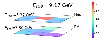
(a)

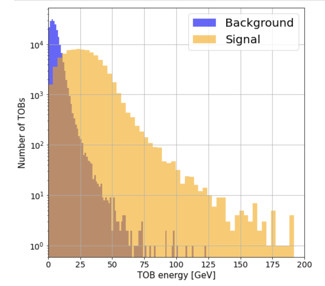
(b)

Figure 1: (a) Layer structure of a reconstructed $3\times 3$ TOB matched to the visible component of a hadronically decaying tau lepton. The $x$ and $y$ axis are the $\Delta\eta$ and $\Delta\phi$ directions and the vertical scale denotes the energy deposited per cell in GeV, also shown per electromagnetic (EM) and hadronic (Had) layers and for the total TOB. (b) Transverse energy of reconstructed TOBs for signal and background samples. All reconstructed TOBs are shown for the background while only TOBs matched to the visible component of a hadronically decaying taus are shown for the signal.

3 Supervised learning training

The classification task addressed in this work belongs to the supervised learning (SL) category. The model is trained to learn a function that maps inputs to outputs using a labeled training dataset. In the following, a single TOB is referred to as a ‘sample’, representing the individual input provided to each model. The problem is approached as a binary classification scenario with a traditional loss function - the Cross-Entropy (CE) metric. To optimize the CE loss function, we employ the (iterative) Stochastic Gradient Descent (SGD) algorithm across all the tested models. In terms of data balance, the ratio of signal to background TOBs was maintained consistently throughout our discussions, with approximately 70k signal TOBs and 200k background TOBs.

We explored three different learning methods: one is a classic machine learning (ML) model, namely a decision tree, while the other two are NN models inspired by the computer vision field - the field that deals with gaining high-level understanding from digital images or videos. Note that while the model inputs are quite similar to those of ‘standard’ NN tasks, in our case there are strict latency and computational constraints that arise from the very high rate of events of the ATLAS experiment. Therefore, the goal is to build architectures as simple as possible that can still be implemented with FPGAs.

The first concept that we have explored is the Extreme Gradient Boosting (XGBoost) algorithm  Chen_2016 which became well known in the ML community after being part of the winning solution of the Higgs Machine Learning Challenge in Kaggle pmlr-v42-cowa14 . XGBoost is a gradient boosting tree model that usually involves a small number of parameters compared to NN models since its inputs are only high level features produced from the raw data, hence allowing a simpler FPGA implementation with minimal computational requirements and low latency inference time Hong:2021snb . The high level features we used for this model describe the most important information about the energy deposits and their positions in the TOB in a single vector of size 17. The strongest features according to feature importance methods were the total energy deposited in the TOB, total energy in each layer, average penetration depth of the energy deposits along the calorimeter, ratio of the cell energies squared to their respective volumes, first and second maximal energy deposits of the second layer and few ratio combinations of all the above-mentioned.

The second architecture is a multi-layer perceptron (MLP) NN, which has the ability to learn linear and non-linear relationships between data elements due to to the neuron’s activation function. Due to simplicity reasons, we used for the MLP a minimal structure of two hidden layers with (5,4) units each. Unlike in XGBoost, the NN employs the entire raw data elements in a flattened shape and not as the raw data structure tensor. In this kind of model, all energy evidences are transferred as inputs but the model does not get explicit spatial information regarding the energy deposit positions in the TOB.

The third approach we study relies on the shape of each TOB and therefore treats it as a tensor - similar to a dual channel matrix, where the pixel values are the energy deposits of the cells. For this ‘image like’ perspective we built an architecture based on the Residual Network (ResNet)  he2015deep , which consists of skip-connections and contains nonlinearities (using the ReLU activation function as in MLP) and batch normalization layers in between. As in NN, the purpose of this architecture is to transfer energy evidence; however, the physical positions of each cell are also taken into account.

4 Results

In this section we discuss the results for the aforementioned architectures using the three aforementioned datasets. All datasets include 200k background and around 70k signal samples (TOBs) but with one distinction - the dataset TOBs have a different cardinality in Hadronic and electo-magnetic layers so we get three tensor dimensions (this is 2 layers (EM,HAD), then the size of the towers): $2\times 3\times 3$, $2\times 5\times 5$ and $2\times 9\times 9$. Prior to the evaluation of each classifier’s performance, we first present the score distribution of the models. In Figure 2 we demonstrate that there is a good separation between signal and background distributions for all the architectures. However, there is a significant difference between XGBoost and NNs in the variance of the distributions for the high dimensional data structure; the XGB background score variance is higher than NNs’ variance, a feature that might suggest a worse signal/background separation and therefore a lower classification quality for this kind of data.

Figure 2: Score distributions for signal (orange) and background (blue) TOBs with $2\times 3\times 3$ (top) and $2\times 9\times 9$ (bottom) dimensions for: left: XGBoost; center: MLP; and right: ResNet;

The performance is evaluated using multiple metrics; first we use the most common classification evaluation metrics, namely, the precision recall curve (PR) and the receiver operating characteristic curve (ROC), which show the performance of a classification model at all classification thresholds by presenting the precision against recall and true positive rate (TPR) against the false positive rate (FPR) respectively for each. For both curves we also measure the area under curve (AUC), which is an aggregated measurement of the prediction quality across all possible thresholds, with higher values corresponding to better classifiers.

In addition to the previous metrics, we tested a more practical and unique metric, which is more adjusted to the needs of the hadron collider experiments such as ATLAS experiment: the Turn-on Curve (TOC), also known as an efficiency plot, and its AUC, the TOC-AUC. The TOC shows the efficiency as a function of a given observable obtained from a given model at the event level, as opposed to both the ROC and PR curves that quantify it at the TOB level. An event, composed of many TOBs, is classified as signal if even a single one of its TOBs is classified by the model as signal. Otherwise, it is classified as background. First, a model threshold is determined by the ‘fake rate’ - the maximum number of background events that can be allowed to be mistakenly classified as signal. The fake rate is dictated by the maximum trigger bandwidth, i.e., the maximal rate of events that can be recorded. Then, given this model threshold, the model efficiency for the signal can be plotted separately for each ${\rm p_{T}}$ range. Since it becomes easier to classify signal events as the $\tau$ energy increases, the TOC efficiency is expected to begin at 0 and approach 1. The quicker the ‘turn-on’ response the more successful the model. In our case, the improvement can be seen in the low ${\rm p_{T}}$ ranges of 10-20 GeV. This means using this method we can detect more low-${\rm p_{T}}$ taus that would otherwise be missed.

Table 1: ROC-AUC, PR-AUC and F1-MAX for each of the architectures and per every data dimension. The metrics shown in bold denote which is the best architecture for each of the data dimensions.

Metric	Granularity	XGBoost	MLP	ResNet
	3$\times$3	0.969	0.967	0.968
ROC_AUC	5$\times$5	0.936	0.93	0.931
	9$\times$9	0.967	0.963	0.964
	3$\times$3	0.956	0.952	0.952
PR_AUC	5$\times$5	0.912	0.903	0.904
	9$\times$9	0.955	0.95	0.952
	3$\times$3	0.898	0.893	0.893
F1_MAX	5$\times$5	0.846	0.836	0.838
	9$\times$9	0.904	0.9	0.902

As can be seen in Table 1, the regular classification metrics reveal only tiny differences in performance between the three architectures in each of the data structures. It also does not describe the performance vs ${\rm p_{T}}$ and is also affected by the high imbalance of our dataset. This is in contrast to Figure 3 that presents the TOC curves, where we can evaluate the efficiency of every method: note that the baseline of our task is a classic algorithm and not an ML one; this algorithm simply looks for clusters in the TOB layers and above a certain threshold classifies the event as a signal. As we can see from the TOC, all ML algorithms have a much higher efficiency for ${\rm p_{T}}$ below 20 GeV and are equal to the baseline performance above this range. The best algorithm in the low ${\rm p_{T}}$ range is changing depending on the data structure we study: in the lowest TOB cardinality $2\times 3\times 3$, the XGBoost performance (in TOC terms for ${\rm p_{T}}$ below 20 GeV) surpasses the NN models. For a slightly higher cardinality of $2\times 5\times 5$, XGBoost still takes the lead, however, the performance gap is reduced. Finally, when we run all models over the biggest data structure $2\times 9\times 9$, the algorithm ranking changes completely with ResNet performance at the top and XGBoost moving to the bottom.

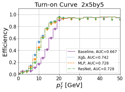
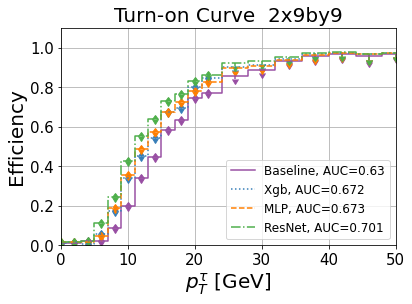
Figure 3: TOC of all architectures with different data dimension

5 Conclusions

The growing rate of $pp$ events at the Large Hadron Collider (LHC) is vital for searching for new phenomena. However, the increasing pace of collected data poses challenges in filtering the relevant events. A novel $\tau$ triggering technique is introduced that is able to significantly improve the ability to trigger on low ${\rm p_{T}}$ hadronically decaying $\tau$s. We introduce a decision tree trained with XGBoost and advanced deep learning techniques such as MLP and ResNet, and demonstrate their ability at different complexity levels of data structures. For most of the energy range considered, ResNet is found to be the best performing technique for high dimensional structure while for low complexity data, a classic ML approach like XGBoost gives the best performance. In the future, LHC experiments can utilize these techniques to accommodate the anticipated conditions, which will involve higher detector granularity and more intricate data structures.

- (1) ATLAS Collaboration, G. Aad et al., The ATLAS Experiment at the CERN Large Hadron Collider, JINST 3 (2008) S08003.
- (2) CMS Collaboration, S. Chatrchyan et al., The CMS Experiment at the CERN LHC, JINST 3 (2008) S08004.
- (3) ATLAS Collaboration, G. Aad et al., Performance of the upgraded PreProcessor of the ATLAS Level-1 Calorimeter Trigger, JINST 15 (2020), no. 11 P11016, [arXiv:2005.04179].
- (4) ATLAS Collaboration, The ATLAS Tau Trigger in Run 2, tech. rep., CERN, Geneva, 2017.
- (5) CMS Collaboration, V. Khachatryan et al., The CMS trigger system, JINST 12 (2017), no. 01 P01020, [arXiv:1609.02366].
- (6) J. Duarte et al., Fast inference of deep neural networks in FPGAs for particle physics, JINST 13 (2018), no. 07 P07027, [arXiv:1804.06913].
- (7) V. Loncar et al., Compressing deep neural networks on FPGAs to binary and ternary precision with HLS4ML, Mach. Learn. Sci. Tech. 2 (2021) 015001, [arXiv:2003.06308].
- (8) B. Carlson, Q. Bayer, T. M. Hong, and S. Roche, Nanosecond machine learning regression with deep boosted decision trees in FPGA for high energy physics, JINST 17 (2022), no. 09 P09039, [arXiv:2207.05602].
- (9) G. C. Branco, P. M. Ferreira, L. Lavoura, M. N. Rebelo, M. Sher, and J. P. Silva, Theory and phenomenology of two-Higgs-doublet models, Phys. Rept. 516 (2012) 1–102, [arXiv:1106.0034].
- (10) A. Djouadi, The Anatomy of electro-weak symmetry breaking. II. The Higgs bosons in the minimal supersymmetric model, Phys. Rept. 459 (2008) 1–241, [hep-ph/0503173].
- (11) CMS Collaboration, A. Tumasyan et al., Identification of hadronic tau lepton decays using a deep neural network, JINST 17 (2022) P07023, [arXiv:2201.08458].
- (12) ATLAS Collaboration, G. Aad et al., Technical Design Report for the Phase-I Upgrade of the ATLAS TDAQ System, .
- (13) Particle Data Group Collaboration, R. L. Workman et al., Review of Particle Physics, PTEP 2022 (2022) 083C01.
- (14) R. Achenbach et al., The ATLAS level-1 calorimeter trigger, JINST 3 (2008) P03001.
- (15) J. Alwall, R. Frederix, S. Frixione, V. Hirschi, F. Maltoni, O. Mattelaer, H. S. Shao, T. Stelzer, P. Torrielli, and M. Zaro, The automated computation of tree-level and next-to-leading order differential cross sections, and their matching to parton shower simulations, JHEP 07 (2014) 079, [arXiv:1405.0301].
- (16) T. Sjöstrand, S. Ask, J. R. Christiansen, R. Corke, N. Desai, P. Ilten, S. Mrenna, S. Prestel, C. O. Rasmussen, and P. Z. Skands, An introduction to PYTHIA 8.2, Comput. Phys. Commun. 191 (2015) 159–177, [arXiv:1410.3012].
- (17) S. Ovyn, X. Rouby, and V. Lemaitre, DELPHES, a framework for fast simulation of a generic collider experiment, arXiv:0903.2225.
- (18) DELPHES 3 Collaboration, J. de Favereau, C. Delaere, P. Demin, A. Giammanco, V. Lemaître, A. Mertens, and M. Selvaggi, DELPHES 3, A modular framework for fast simulation of a generic collider experiment, JHEP 02 (2014) 057, [arXiv:1307.6346].
- (19) “Delphes: A framework for fast simulation of a generic collider experiment.”
- (20) T. Chen and C. Guestrin, XGBoost, in Proceedings of the 22nd ACM SIGKDD International Conference on Knowledge Discovery and Data Mining, ACM, aug, 2016.
- (21) C. Adam-Bourdarios, G. Cowan, C. Germain, I. Guyon, B. Kégl, and D. Rousseau, The Higgs boson machine learning challenge, in Proceedings of the NIPS 2014 Workshop on High-energy Physics and Machine Learning (G. Cowan, C. Germain, I. Guyon, B. Kégl, and D. Rousseau, eds.), vol. 42 of Proceedings of Machine Learning Research, (Montreal, Canada), pp. 19–55, PMLR, 13 Dec, 2015.
- (22) T. M. Hong, B. Carlson, B. Eubanks, S. Racz, S. Roche, J. Stelzer, and D. Stumpp, Nanosecond machine learning event classification with boosted decision trees in FPGA for high energy physics, JINST 16 (2021), no. 08 P08016, [arXiv:2104.03408].
- (23) K. He, X. Zhang, S. Ren, and J. Sun, Deep residual learning for image recognition, 2015.