The strong decay of $Y(4230)\to J/\psi f_{0}(980)$ in light cone sum rules

Abstract

In this work, we assign the tetraquark state for $Y(4230)$ resonance, and investigate the mass and decay constant of $Y(4230)$ in the framework of SVZ sum rules through a different calculation technique. Then we calculate the strong coupling $g_{YJ/\psi f_{0}}$ by considering soft-meson approximation techniques, within the framework of light cone sum rules. And we use strong coupling $g_{YJ/\psi f_{0}}$ to obtain the width of the decay $Y(4230)\to J/\psi f_{0}(980)$. Our prediction for the mass is in agreement with the experimental measurement, and that for the decay width of $Y(4230)\to J/\psi f_{0}(980)$ is within the upper limit.

I Introduction

$Y(4230)$ a.k.a. $\psi(4230)$ is the first observed $Y$ state which was detected through initial-state-radiation (ISR) technique in the process $e^{+}e^{-}\to$ $J/\psi\pi^{+}\pi^{-}$ by the BABAR experiment in 2005 Aubert et al. (2005), and then confirmed by the CLEO He et al. (2006) and the Belle Yuan et al. (2007) in the same process. An accumulation of events with similar characteristics was reported in other two processes $e^{+}e^{-}\to$ $J/\psi\pi^{0}\pi^{0}$ (and $J/\psi K^{+}K^{-}$) by the CLEO Coan et al. (2006), and also in the decay of $B^{-}\to$ $\psi$(4230)$K^{-}\to J/\psi\pi^{+}\pi^{-}K^{-}$ by BABAR Lees et al. (2012) collaboration.

In 2017, the BESIII collaboration has announced a new precise measurement of the $e^{+}e^{-}\to J/\psi\pi^{+}\pi^{-}$ cross section Ablikim et al. (2017), reporting updated values for the mass and the width of the $Y(4230)$. Particularly, a second resonance is also presented in the $J/\psi\pi^{+}\pi^{-}$ mass spectrum. The values of the two observed resonances are, respectively: $(4222.0\pm 3.1\pm 1.4)$ and $(44.1\pm 4.3\pm 2.0)$ MeV for $Y(4230)$; $(4320.0\pm 10.4\pm 7)$ and $(101.4^{+25.3}_{-19.7}\pm 10.2)$ MeV for, namely, $Y(4360)$. Although Ref.Ablikim et al. (2017) proposes that the structure around 4260 MeV could be read as a superposition of these two resonances, and Ref.Ablikim et al. (2019) further suggests them as $Y(4230)$ and $Y(4360)$ respectively, this discussion has not yet settled. Here in our paper we still concentrate on the $Y(4230)$ resonsant state instead of discussing the combined structure.

Experimentally the $Y(4230)$ is directly produced in $e^{+}e^{-}$ annihilation, its spin-parity quantum number should be $J^{PC}=1^{--}$, which is consistent with that of a vector charmonium state. Theorists have tried to categorize it into the vector charmonium group. However, on account of its mass does not fit any mass of charmonium states in the same mass region, and that $c\bar{c}$ mainly decay to $D^{(*)}\bar{D}^{(*)}$, but the observed $Y$ in such decay does not match the peaks in the $e^{+}e^{-}\to D^{(*)\pm}D^{(*)\mp}$ cross sections measured by the BABAR Ablikim et al. (2019); Pakhlova et al. (2008) and the Belle Abe et al. (2007) collaborations, the $Y$(4230) does not look like a normal $c\bar{c}$ state. Furthermore, for the $1^{--}$ radially excited charmoniums, four of the $S$-wave states: $\psi(1S)$, $\psi(2S)$, $\psi(3S)$ and $\psi(4S)$, have already been assigned to $J/\psi$, $\psi(3686)$, $\psi(4040)$ and $\psi(4415)$ mesons, respectively, and two of the $D$-wave states $\psi(1D)$ and $\psi(2D)$ have been assigned to $\psi(3770)$ and $\psi(4160)$ mesons. In addition, the masses of $\psi(5S)$ and $\psi(3D)$ states in the quark model are 4.76 and 4.52 GeV, and thus higher than that of the $Y(4230)$. According to the above analysis, one can reach that $Y(4230)$ may not consistent with any of the $1^{--}$ $c\bar{c}$ states Zhu (2008); Klempt and Zaitsev (2007); Nielsen et al. (2010).

To further explain the structure of $Y(4230)$, many theoretical interpretations have been to emerge, including a tetraquark state Maiani et al. (2005); Zhu (2005); Albuquerque and Nielsen (2009); Ebert et al. (2008), a compact tetraquark state Maiani et al. (2014), a hadrocharmonium state Li and Voloshin (2014); Dubynskiy and Voloshin (2008), hadronic molecule of $D_{0}\bar{D}^{*}$, $D_{1}D$, $D_{0}D^{*}$ or $\bar{D}D_{1}(2420)$ Albuquerque and Nielsen (2009); Ding (2009); Wang et al. (2013); Cleven et al. (2014), $\chi_{c1}\omega$ Yuan et al. (2006), $\chi_{c1}\rho$ Liu et al. (2005), $J/\psi K\bar{K}$ Martinez Torres et al. (2009), $\psi^{\prime}f_{0}(980)$Guo et al. (2008a), a $c\bar{c}$-gluon hybrid Zhu (2005); Close and Page (2005); Kou and Pene (2005), a charm baryonium Qiao (2006), a coupled-channel model van Beveren and Rupp (2006, 2009), etc. However, within the available experimental data, none of these theoretical interpretations can be completely accepted or excluded to the nature of $Y(4230)$.

For example, if it’s in the compact tetraquark model Maiani et al. (2013), there exists an isospin-violating process $Y(4230)\to\eta\pi^{0}J/\psi$ with a sizeable decay width, where both $\pi^{0}J/\psi$ and $\eta J/\psi$ can be produced from $Z_{c}^{0}$ decay. Therefore, the interpretation of $Y(4230)$ in the compact tetraquark model can lead to a peak in $e^{+}e^{-}\to\eta\pi^{0}J/\psi$ cross section and a very prominent peak should appear in $\eta J/\psi$ mass spectrum between the $D\bar{D}^{*}$ thereshold Wu et al. (2014). However, using the datas from the BESIII experiment searching for isospin-violating Ablikim et al. (2015), no $Y(4230)$ signal is observed. Besides, whatever it is in the compact tetraquark model it should have isospin and SU(3)-multiplet partner states. But none of those partners for $\psi$(4230) has been observed in experiments so far. If $\psi$(4230) is a hadrocharmonium, it’s structure would be formed with the mixing of another hadrocharmonia. These two hadrocharmonia states contain spin 1 and spin 0 compact $c\bar{c}$ cores respectively Li and Voloshin (2014). However, based on BESIII data Ablikim et al. (2017) the decay rate of $Y(4230)$ to non-$J/\psi(h_{c})$ charmonium states should be suppressed Li and Voloshin (2014), indicating that the above suggestion may not consistent. If we assign the $\bar{D}D_{1}(2420)$ molecule to $\psi$(4230), the binding energy being about 66 MeV is rather large, though this possibility is not excluded Brambilla et al. (2020). There are other candidates for $\psi$(4230), e.g., $\bar{D}D_{1}(2430)$, $\bar{D}^{*}D_{0}$, $\bar{D}_{s0}D_{s}^{*}$, $\bar{D}_{s}D_{s1}$, whose open charm thresholds are around 4.26 GeV with $J^{PC}=1^{--}$. Unfortunately, beside $\bar{D}_{s0}D_{s}^{*}$, their widths are too broad to make a bound state so that could not be consistent with the total decay width of $Y(4230)$ Wang et al. (2013); Beringer et al. (2012). For the $\bar{D}_{s0}D_{s}^{*}$ molecular, its mass is $4.42\pm 0.10$ GeV, which should also be excluded Albuquerque and Nielsen (2009). Anyway, $Y$(4230) seems not a hadronic molecule.

The $Y(4230)$ may also be assumed as a charmonium hybrid meson. However, in Ref.Guo et al. (2008b) the authors find that the mass of $1^{--}$ hybrid states lie at $4.47$ GeV, heavier than the mass of the $Y(4230)$. In non-relativistic EFTs, the mass of $Y(4230)$ may consistent with one state of $H_{1}$ hybrid multiplet, but $Y(4230)$ disfavors the hybrid interpretation since it decays to spin triplet charmonium while $H_{1}$ is only a spin singlet Berwein et al. (2015). In Ref.Ma et al. (2021), it was found that the color halo picture is compatible with $Y(4260)$ decay properties, and suggests LHCb and BelleII to search for $(0,1,2)^{+-}$ charmonium-like hybrids in $\xi_{c0,1,2}\eta$ and $J/\psi\omega(\psi)$ final states. We should not jump to the conclusion that $Y(4230)$ can not be the hybrid state.

In summary, at this point the structure of $Y(4230)$ is not yet fully settled.

In this paper we investigate the strong decay of $Y(4230)\to$ $J/\psi f_{0}(980)$ observed in the process $e^{+}e^{-}\to J/\psi\pi^{+}\pi^{-}$. Notice $Y(4230)$ will decay into a $f_{0}(980)$ which fits the $S$-wave $[sq][\bar{s}\bar{q}]$ hypothesis Maiani et al. (2004). Furthermore, being a member of vector charmonium family suggests $\psi$(4230) a $[cs][\bar{c}\bar{s}]$ composition. We therefore consider $Y(4230)$ as a tetraquark state, as in Ref.Dubnička et al. (2020). This differs from other ideas, i.e., in Ref.Albuquerque et al. (2011) the $Y(4230)$ was suggested to be a $J/\psi f_{0}(980)$ bound system. We calculate the strong coupling $g_{YJ/\psi f_{0}}$ by using the method of light cone sum rules, with the interpolating current taken from Ref.Albuquerque and Nielsen (2009). We evaluate the mass of $Y(4230)$ through a different calculation technique developed in Ref.Azizi et al. (2018), not the usual way in two-point sum rules Agaev et al. (2017a). Compare the mass prediction of $Y(4230)$ with the result in PDG Zyla et al. (2020), we confirm our technique generalization is credible. We then extend it to evaluate the decay constant of $Y(4230)$ which will be used in the numerical calculation of the strong coupling $g_{YJ/\psi f_{0}}$. Finally, the decay width of $Y(4230)\to J/\psi f_{0}(980)$ is obtained, and further results are compared with the experimental measurement and discussed.

Our work is organized as follows:

In Section.II we calculate the mass and decay constant of the $Y(4230)$ state within two-point sum rule approach develop by Shifman, Vainshtein and Zakharov (SVZ sum rules) Shifman et al. (1979). And we also calculate the strong coupling $g_{YJ/\psi f_{0}}$ will be derived with the approach of light cone sum rules. The numerical results and discussions are shown in Section.III. We reach our summary in Section.IV

II Calculation Framework

II.1 The mass and the decay constant of $Y(4230)$

We begin by calculating the mass and the decay constant using the two-point correlation function:

$$\Pi_{\mu\nu}(p)=i\int\mbox{d}^{4}xe^{ipx}\braket{0}{T\{J_{\mu}^{Y}(x)J_{\nu}^{Y\dagger}(0)\}}{0},$$ (1)

where the interpolating currents are given in the following expression:

$$J_{\mu}^{Y}(x) =\frac{\varepsilon_{abc}\varepsilon_{dec}}{\sqrt{2}}\{[s^{T}_{a}(x)C\gamma_{5}c_{b}(x)][\bar{s}_{d}(x)\gamma_{\mu}\gamma_{5}C\bar{c}_{e}^{T}(x)]$$ (2)

$$-[s_{a}^{T}(x)C\gamma_{\mu}\gamma_{5}c_{b}(x)][\bar{s}_{d}(x)\gamma_{5}C\bar{c}_{e}^{T}(x)]\},$$

$$J^{Y\dagger}_{\nu}(0) =\frac{\varepsilon_{abc}\varepsilon_{dec}}{\sqrt{2}}\{-[\bar{c}_{b}(0)\gamma_{5}C\bar{s}_{a}^{T}(0)][c_{e}^{T}(0)C\gamma_{\nu}\gamma_{5}s_{d}(0)]$$

$$+[\bar{c}_{b}(0)\gamma_{\nu}\gamma_{5}C\bar{s}_{a}^{T}(0)][c_{e}^{T}(0)C\gamma_{5}s_{d}(0)]\}.$$

As a first step, we calculate the correlation function by inserting a complete set of hadronic states into Eq.(1):

$$\Pi^{\text{h}}_{\mu\nu}(p) =\frac{\braket{0}{J_{\mu}^{Y}}{Y(p)}\braket{Y(p)}{J_{\mu}^{Y\dagger}}{0}}{m_{Y}^{2}-p^{2}}+\int_{s^{\prime}}^{\infty}d\hat{s}\frac{\rho_{\mu\nu}^{\text{h}}(\hat{s})}{\hat{s}-p^{2}},$$ (3)

where the higher resonances and continuous states are represented by $\rho_{\mu\nu}^{\text{h}}(\hat{s})$. Due to the fact that they would disappear following the Borel transformation, the subtraction terms are not displayed. We define the decay constant $f_{Y}$ according to

$$\braket{0}{J_{\mu}^{Y}}{Y(p)}=m_{Y}f_{Y}\epsilon_{\mu}$$ (4)

with $\epsilon_{\mu}$ being the polarization vector of $Y(4230)$. After performing the polarization sum equation we can obtain

$$\Pi_{\mu\nu}^{\text{h}}(p)=\frac{m_{Y}^{2}f_{Y}^{2}}{m_{Y}^{2}-p^{2}}(-g_{\mu\nu}+\frac{p_{\mu}p_{\nu}}{m_{Y}^{2}})+\int_{s^{\prime}}^{\infty}d\hat{s}\frac{\rho_{\mu\nu}^{\text{h}}(\hat{s})}{\hat{s}-p^{2}}.$$ (5)

On the right side of Eq.(5), we are beginning to observe a pole. The Borel transformation can be performed on Eq.(5) to remove the pole, which yields

$$\Pi_{\mu\nu}^{\text{h}}(M^{2})=$$ (6)

$$m_{Y}^{2}f_{Y}^{2}e^{-m_{Y}^{2}/M^{2}}(-g_{\mu\nu}+\frac{p_{\mu}p_{\nu}}{m_{Y}^{2}})+\int_{s^{\prime}}^{\infty}d\hat{s}\rho_{\mu\nu}^{\text{h}}(\hat{s})e^{-\hat{s}/M^{2}}.$$

Next, let’s consider the correlation function in the OPE side. Following Wick Theorm contraction of the heavy and light quarks, we obtain:

$$\Pi_{\mu\nu}^{\text{OPE}}(p)=\frac{1}{2}\int\mbox{d}^{4}xe^{ipx}\epsilon_{abc}\epsilon_{dec}\epsilon_{a^{\prime}b^{\prime}c^{\prime}}\epsilon_{d^{\prime}e^{\prime}c^{\prime}}$$ (7)

$$-\text{Tr}[\tilde{S}^{aa^{\prime}}_{s}(x)\gamma_{5}S_{c}^{bb^{\prime}}(x)\gamma_{5}]\text{Tr}[S^{dd^{\prime}}_{s}(-x)\gamma_{\mu}\gamma_{5}\tilde{S}_{c}^{ee^{\prime}}(-x)\gamma_{\nu}\gamma_{5}]$$

$$+\text{Tr}[\tilde{S}^{aa^{\prime}}_{s}(x)\gamma_{5}S_{c}^{bb^{\prime}}(x)\gamma_{\nu}\gamma_{5}]\text{Tr}[S^{dd^{\prime}}_{s}(-x)\gamma_{\mu}\gamma_{5}\tilde{S}_{c}^{ee^{\prime}}(-x)\gamma_{5}]$$

$$+\text{Tr}[\tilde{S}^{aa^{\prime}}_{s}(x)\gamma_{\mu}\gamma_{5}S_{c}^{bb^{\prime}}(x)\gamma_{5}]\text{Tr}[S^{dd^{\prime}}_{s}(-x)\gamma_{5}\tilde{S}_{c}^{ee^{\prime}}(-x)\gamma_{\nu}\gamma_{5}]$$

$$-\text{Tr}[\tilde{S}^{aa^{\prime}}_{s}(x)\gamma_{\mu}\gamma_{5}S_{c}^{bb^{\prime}}(x)\gamma_{\nu}\gamma_{5}]\text{Tr}[S^{dd^{\prime}}_{s}(-x)\gamma_{5}\tilde{S}_{c}^{ee^{\prime}}(-x)\gamma_{5}],$$

where $\tilde{S}_{q}^{ab}(x)$ represent $CS_{q}^{ab}(x)C$. We accept the following expression for propagators of the $u$, $d$, and $s$ quarks in coordinate-spaceHuang et al. (2011); Agaev et al. (2016a)

$$S_{q,ab}(x) =\frac{i\delta_{ab}\not{x}}{2\pi^{2}x^{4}}-\frac{\delta_{ab}m_{q}}{4\pi^{2}x^{2}}-\frac{{\langle\bar{q}q\rangle}}{12}$$ (8)

$$-\frac{i}{32\pi^{2}}\frac{\lambda^{n}}{2}g_{s}G_{\mu\nu}^{n}\frac{1}{x^{2}}(\sigma^{\mu\nu}\not{x}+\not{x}\sigma^{\mu\nu})$$

$$+\frac{i\delta_{ab}\not{x}m_{q}{\langle\bar{q}q\rangle}}{48}-\frac{\delta_{ab}{\langle\bar{q}g_{s}\sigma Gq\rangle}x^{2}}{192}$$

$$+\frac{i\delta_{ab}x^{2}\not{x}m_{q}\langle\bar{q}g_{s}\sigma Gq\rangle}{1152}$$

$$-\frac{i\delta_{ab}x^{2}\not{x}g_{s}^{2}\langle\bar{q}q\rangle^{2}}{7776}-\frac{\delta_{ab}x^{4}\langle\bar{q}q\rangle\langle g_{s}^{2}GG\rangle}{27648}.$$

The heavy quark propagator is given, in terms of the second kind Bessel functions $K_{v}(x)$, as Aliev et al. (2016):

$$S^{ab}_{c}(x)=\frac{m_{Q}^{2}}{4\pi^{2}}[\frac{K_{1}(m_{Q}\sqrt{-x^{2}})}{\sqrt{-x^{2}}}\delta_{ab}+i\frac{\not{x}K_{2}(m_{Q}\sqrt{-x^{2}})}{(\sqrt{-x^{2}})^{2}}\delta_{ab}]$$ (9)

$$-\frac{g_{s}m_{Q}}{16\pi^{2}}\int_{0}^{1}\mbox{d}vG^{\mu\nu}_{ab}(vx)[(\sigma_{\mu\nu}\not{x}+\not{x}\sigma_{\mu\nu})\frac{K_{1}(m_{Q}\sqrt{-x^{2}})}{\sqrt{-x^{2}}}$$

$$+2\sigma^{\mu\nu}K_{0}(m_{Q}\sqrt{-x^{2}})].$$

Notice the heavy quark propagator here is different from the expression presented in the usual way, for example in Ref.Agaev et al. (2017a), where the heavy quark propagator is expressed in the momentum space. If use momentum expression of propagator in Eq.(7), we have to face divergences in the double integrals like

$$\int\frac{d^{4}k_{1}d^{4}k_{2}}{(k_{1}^{2}-m_{c}^{2})(k_{2}^{2}-m_{c}^{2})}.$$ (10)

As shown in Ref.Azizi et al. (2018), by using an appropriate representation of the modified Bessel functions in heavy quark propagator, like in Eq.(9), results without any divergences can be obtained. Since here we are using the SVZ sum rules instead of the LCSR, we have to modify the calculation when the paticle distribution function do not participate in Eq(7). We showe the details of the modification in Appendix V.3.

The correlation function $\Pi^{\text{OPE}}_{\mu\nu}(p)$ has also the following decomposition over the Lorentz structures

$$\Pi^{\text{OPE}}_{\mu\nu}(p)=\Pi^{\text{OPE}}(p)g_{\mu\nu}+\widetilde{\Pi}^{\text{OPE}}(p)p_{\mu}p_{\nu},$$ (11)

and we choose to work with the term $\sim g_{\mu\nu}$, which can be represented as the dispersion integral

$$\widetilde{\Pi}^{\text{OPE}}(p)=\int_{4m_{c}^{2}}^{\infty}\mbox{d}\hat{s}\frac{\rho^{\text{OPE}}(\hat{s})}{\hat{s}-p^{2}},$$ (12)

where $\rho^{\text{OPE}}(\hat{s})$ is the corresponding spectral density.

The Borel transformation and the quark-hadron duality can be applied to $\widetilde{\Pi}^{\text{OPE}}(p)$ to obtain:

$$p_{\mu}p_{\nu}\int_{4m_{c}^{2}}^{\infty}\mbox{d}\hat{s}\rho^{\text{OPE}}(\hat{s})e^{-\hat{s}/M^{2}}=$$ (13)

$$m_{Y}^{2}f_{Y}^{2}e^{-m_{Y}^{2}/M^{2}}(\frac{p_{\mu}p_{\nu}}{m_{Y}^{2}})+p_{\mu}p_{\nu}\int_{s_{0}}^{\infty}\rho^{\text{h}}(\hat{s})e^{-\hat{s}/M^{2}}.$$

Next, take out the contribution from the continuum to get:

$$f_{Y}^{2}e^{-m_{Y}^{2}/M^{2}}=\int_{4m_{c}^{2}}^{s_{0}}\mbox{d}\hat{s}\rho^{\text{OPE}}(\hat{s})e^{-\hat{s}/M^{2}}.$$ (14)

The $Y(4230)$ state mass can be determined by the sum rule

$$m_{Y}^{2}=\frac{\int_{4m_{c}^{2}}^{s_{0}}\mbox{d}\hat{s}\hat{s}\rho^{\text{OPE}}(\hat{s})e^{-\hat{s}/M^{2}}}{\int_{4m_{c}^{2}}^{s_{0}}\mbox{d}\hat{s}\rho^{\text{OPE}}(\hat{s})e^{-\hat{s}/M^{2}}}.$$ (15)

II.2 The strong coupling $g_{YJ/\psi f_{0}}$ in light cone sum rules

It is necessary to calculate the strong coupling $g_{YJ/\psi f_{0}}$ first, based on the light cone sum rules(LCSR), before predicting the width of $Y(4230)\to J/\psi f_{0}(980)$. We begin by using the two-point correlation function:

$$\Pi_{\mu\nu}(p^{\prime},q)=i\int\mbox{d}^{4}xe^{ipx}\braket{f_{0}(q)}{T\{J_{\mu}^{J/\psi}(x)J_{\nu}^{Y\dagger}(0)\}}{0},$$ (16)

where $f_{0}$ represents the scalar meson $f_{0}(980)$. $Y(4230)$ has momentum $p^{\prime}=p+q$, and $p$, $q$ represent the four-momentum for $J/psi$ and $f_{0}$, respectively. $J_{\mu}^{J/\psi}$ is the interpolating current of $J/\psi$ given by Albuquerque and Nielsen (2009); Bečirević et al. (2014)

$$J_{\mu}^{J/\psi}(x)=\bar{c}_{i}(x)\gamma_{\mu}c_{i}(x).$$ (17)

here $i$ denotes the color indexes and $C$ is the charge conjugation matrix.

II.2.1 Phenomenological side calculation

Next, we must build a relationship between the correlation function $\Pi_{\mu\nu}(p^{\prime},q)$ and the strong coupling $g_{YJ/\psi f_{0}}$.

By adding two complete sets of hadronic states to Eq.(16), we are able to construct the phenomenological expression of the correlation function:

$$\Pi^{\text{h}}_{\mu\nu}(p^{\prime},q)=$$ (18)

$$\frac{\braket{0}{J_{\mu}^{J/\psi}}{J/\psi(p)}\braket{f_{0}(q)J/\psi(p)}{Y(p^{\prime})}\braket{Y(p^{\prime})}{J_{\nu}^{Y\dagger}}{0}}{(p^{\prime 2}-m_{Y}^{2})(p^{2}-m_{J/\psi}^{2})}$$

$$+\int_{s_{1}^{\prime}}^{\infty}\int_{s_{2}^{\prime}}^{\infty}\frac{ds_{1}ds_{2}\ \rho_{\mu\nu}^{\text{h}}(s_{1},s_{2})}{(s_{1}-p^{2})(s_{2}-p^{\prime 2})}+\cdots,$$

where $\rho_{\mu\nu}^{\text{h}}(s_{1},s_{2})$ represents the contributions of the continuum states and higher resonances, the lowest continuum state thresholds are indicated by the symbols $s_{1}^{\prime}$ and $s_{2}^{\prime}$.

By parameterizing the hadronic matrix element

$$\braket{0}{J_{\mu}^{J/\psi}}{J/\psi(p)}=m_{J/\psi}f_{J/\psi}\varepsilon_{\mu},$$ (19)

$$\braket{Y(p^{\prime})}{J_{\nu}^{Y\dagger}}{0}=m_{Y}f_{Y}\varepsilon_{\nu}^{\prime*},$$

$$\braket{f_{0}(q)J/\psi(p)}{Y(p^{\prime})}=g_{YJ/\psi f_{0}}$$

$$\times ((p^{\prime}\cdot p)(\varepsilon^{*}\cdot\varepsilon^{\prime})-(p^{\prime}\cdot\varepsilon^{*})(p\cdot\varepsilon^{\prime})),$$

and perform the polarization sum, we can easily show that

$$\Pi^{\text{h}}_{\mu\nu}(p^{\prime},q) =\frac{m_{J/\psi}m_{Y}f_{J/\psi}f_{Y}g_{YJ/\psi f_{0}}}{(p^{2}-m_{J/\psi}^{2})(p^{\prime 2}-m_{Y}^{2})}$$ (20)

$$\times[\frac{(m_{J/\psi}^{2}+m_{Y}^{2})}{2}g_{\mu\nu}-p^{\prime}_{\mu}p_{\nu}]+\cdots$$

$$=\Pi^{\text{Phys}}(p^{\prime},q)g_{\mu\nu}+\widetilde{\Pi}^{\text{Phys}}(p^{\prime},q)p^{\prime}_{\mu}p_{\nu},$$

where $m_{J/\psi}$ and $m_{Y}$ are the mass of $J/\psi$ and $Y(4230)$ respectively. $\varepsilon$ and $\varepsilon^{\prime}$ denote the polarization vector of the $J/\psi$ and $Y(4230)$, respectively. $g_{YJ/\psi f_{0}}$ is the invariant constant parameterizing the hadronic matrix element.

In this study, we choose to proceed with a structure that is proportional to $g_{\mu\nu}$

$$\Pi^{\text{h}}(p^{\prime},q) =\frac{m_{J/\psi}m_{Y}f_{J/\psi}f_{Y}g_{YJ/\psi f_{0}}m^{2}}{(p^{2}-m_{J/\psi}^{2})(p^{\prime 2}-m_{Y}^{2})}$$ (21)

$$+\int_{s_{1}^{\prime}}^{\infty}\int_{s_{2}^{\prime}}^{\infty}\frac{\mbox{d}s_{1}\mbox{d}s_{2}\rho^{\text{h}}(s_{1},s_{2})}{(s_{1}-p^{2})(s_{2}-p^{\prime 2})}+\cdots,$$

where we define $m^{2}$ $=\frac{m_{J/\psi}^{2}+m_{Y}^{2}}{2}$. The correlation function Eq.(21) can be transformed into an equation below by applying the Borel transformations to the variables $p^{2}$ and $p^{\prime 2}=(p+q)^{2}$,

$$\mathcal{B}_{p^{2}}(M_{1}^{2})\mathcal{B}_{p^{\prime 2}}(M_{2}^{2})\Pi^{\text{h}}(p^{\prime},q)=$$ (22)

$$m_{J/\psi}m_{Y}f_{J/\psi}f_{Y}g_{YJ/\psi f_{0}}m^{2}\exp[-\frac{m_{J/\psi}}{M_{1}^{2}}-\frac{m_{Y}}{M_{2}^{2}}]$$

$$+\int_{s_{1}^{\prime}}^{\infty}\int_{s_{2}^{\prime}}^{\infty}\mbox{d}s_{1}\mbox{d}s_{2}\exp[-\frac{s_{1}}{M_{1}^{2}}-\frac{s_{2}}{M_{2}^{2}}]\rho^{\text{h}}(s_{1},s_{2}).$$

Since we have the following formula for a general dispersion relation:

$$\Pi_{\mu\nu}(p^{\prime},q)=\frac{1}{\pi^{2}}\int\int\frac{ds_{1}ds_{2}\text{Im}\Pi_{\mu\nu}(s_{1},s_{2})}{(s_{1}-p^{2})(s_{2}-p^{\prime 2})}+\cdots,$$ (23)

where the subtraction terms and single dispersion integrals aren’t provided due to they’ll all vanish when the double Borel transformation is applied to Eq.(23). By choosing to proceed with a structure that is proportional to $g_{\mu\nu}$, we can represent the OPE result for the correlation function as

$$\Pi^{\text{OPE}}(p^{\prime},q)=\int\int\frac{ds_{1}ds_{2}\ \rho^{\text{OPE}}(s_{1},s_{2})}{(s_{1}-p^{2})(s_{2}-p^{\prime 2})},+\cdots$$ (24)

where

$$\rho_{\mu\nu}^{\text{OPE}}(s_{1},s_{2})=\frac{\text{Im}\Pi(s_{1},s_{2})}{\pi^{2}}.$$ (25)

After performing the Borel transformations, we can derive

$$\Pi^{\text{OPE}} (M_{1}^{2},M_{2}^{2})=$$ (26)

$$\int\int\mbox{d}s_{1}\mbox{d}s_{2}\exp[-\frac{s_{1}}{M_{1}^{2}}-\frac{s_{2}}{M_{2}^{2}}]\rho^{\text{OPE}}(s_{1},s_{2}).$$

This is then accomplished by applying the quark-hadron duality, which allows the integral of the hadronic spectral density to equal that of the OPE spectral density, in a certain region:

$$\int_{s_{1}^{\prime}}^{\infty}\int_{s_{2}^{\prime}}^{\infty}\mbox{d}s_{1}\mbox{d}s_{2}\exp[-\frac{s_{1}}{M_{1}^{2}}-\frac{s_{2}}{M_{2}^{2}}]\rho^{\text{h}}(s_{1},s_{2})=$$ (27)

$$\int_{s_{1}^{0}}^{\infty}\int_{s_{2}^{0}}^{\infty}\mbox{d}s_{1}\mbox{d}s_{2}\exp[-\frac{s_{1}}{M_{1}^{2}}-\frac{s_{2}}{M_{2}^{2}}]\rho^{\text{OPE}}(s_{1},s_{2}).$$

After equating (22) and (26), and substituting with (27), we get the following equation for the strong coupling:

$$g_{YJ/\psi f_{0}}=\frac{1}{m_{J/\psi}m_{Y}f_{J/\psi}f_{Y}m^{2}}\exp[\frac{m_{J/\psi}}{M_{1}^{2}}+\frac{m_{Y}}{M_{2}^{2}}]$$ (28)

$$\times\int^{s_{1}^{0}}_{4m_{c}^{2}}\int^{s_{2}^{4m_{c}^{2}}}_{0}\mbox{d}s_{1}\mbox{d}s_{2}\exp[-\frac{s_{1}}{M_{1}^{2}}-\frac{s_{2}}{M_{2}^{2}}]\rho^{\text{OPE}}(s_{1},s_{2}).$$

As we can see from Eq.(16), since the interpolating currents of $Y(4230)$ and $J/psi$ are located at the point $x$ and $0$, respectively, there will still be a quark element $\braket{f_{0}(q)}{[\bar{s}(0)s(0)]}{0}$ after the $\bar{c}$ and $c$ quark fields are contracted. Because $\braket{f_{0}(q)}{[\bar{s}(x)s(0)]}{0}$ will disappears and reduces to normalization factors when $x\to 0$. This situation can be replace by the kinematical limit $q\rightarrow 0$ which call soft-meson approximationBelyaev et al. (1995). Such approximation leads hadronic representation to

$$\Pi^{\text{h}}(p^{\prime},q)=\frac{m_{J/\psi}m_{Y}f_{J/\psi}f_{Y}m^{2}}{(p^{2}-m^{2})^{2}}g_{YJ/\psi f_{0}}+\cdots,$$ (29)

and the Borel transformation on the variable $p^{2}$ applied to this correlation function yields

$$\Pi^{\text{h}}(p^{\prime},q)=m_{J/\psi}m_{Y}f_{J/\psi}f_{Y}\frac{m^{2}}{M^{2}}g_{YJ/\psi f_{0}}e^{-\frac{m^{2}}{M^{2}}}+\cdots,$$ (30)

Following Ioffe and Smilga (1984); Belyaev et al. (1995), we apply the operator

$$(1-\frac{1}{M^{2}})M^{2}e^{m^{2}/M^{2}}$$ (31)

on both sides of the sum rules expression to remove unsuppressed contributions, we can obtain

$$g_{YJ/\psi f_{0}}=\frac{1}{m_{J/\psi}m_{Y}f_{J/\psi}f_{Y}m^{2}}(1-\frac{1}{M^{2}})M^{2}e^{m^{2}/M^{2}}$$ (32)

$$\times\int^{s_{0}}_{4m_{c}^{2}}\mbox{d}\hat{s}\exp[\frac{m_{J/\psi}}{2M^{2}}+\frac{m_{Y}}{2M^{2}}-\frac{\hat{s}}{M^{2}}]\rho^{\text{OPE}}(\hat{s}),$$

which depends only on $\hat{s}$ due to the soft-meson approximation.

II.2.2 OPE side calculation

Taking into account that $g_{XJ/\psi\phi}$ has a relationship to the OPE part of the correlation function, we will calculate it. According to the Wick Theorm, we can derive

$$\Pi_{\mu\nu}(p^{\prime},q) =i\int d^{4}xe^{ipx}\braket{f_{0}(q)}{T\{J_{\mu}^{J/\psi}(x)J_{\nu}^{Y\dagger}(0)\}}{0}$$ (33)

$$=i\int d^{4}xe^{ipx}\frac{\varepsilon_{abc}\varepsilon_{dec}}{\sqrt{2}}\braket{f_{0}(q)}{[\bar{s}^{a}_{\alpha}(0)s^{d}_{\beta}(0)]}{0}$$

$$\times[(\gamma_{5})\tilde{S}^{ib}_{c}(x)\gamma_{\mu}\tilde{S}^{ie}_{c}(-x)\gamma_{\nu}\gamma_{5}$$

$$-(\gamma_{\nu}\gamma_{5})\tilde{S}^{ib}_{c}(x)\gamma_{\mu}\tilde{S}^{ie}_{c}(-x)\gamma_{5}]_{\alpha\beta}.$$

For the heavy quark propagator on the light cone we employ its expression in terms of Agaev et al. (2017b)

$$S^{ab}_{c}(x)= i\int\frac{d^{4}k}{(2\pi)^{4}}e^{-ikx}$$ (34)

$$[ \frac{\delta_{ab}(\not{k}+m_{c})}{k^{2}-m^{2}_{c}}-\frac{g_{s}G_{ab}^{\alpha\beta}}{4}\frac{\sigma_{\alpha\beta}(\not{k}+m)+(\not{k}+m)\sigma_{\alpha\beta}}{(k^{2}-m^{2})^{2}}],$$

where we adopt the notation

$$G_{ab}^{\mu\nu}\equiv G_{i}^{\mu\nu}t^{i}_{ab},i=1,2,\cdots,8.$$ (35)

Substituting the summation and the expansion

$$\bar{s}^{d}_{\alpha}(0)s^{d^{\prime}}_{\beta}(0)=\frac{1}{3}\delta_{dd^{\prime}}\bar{s}_{\alpha}(0)s_{\beta}(0),$$ (36)

$$\bar{s}_{\alpha}(0)s_{\beta}(0)\equiv\frac{1}{4}\Gamma^{j}_{\alpha\beta}\bar{s}(0)\Gamma^{j}s(0),$$

into Eq.(33), we can obtain

$$\Pi_{\mu\nu}(p^{\prime},q) =i\int\mbox{d}^{4}xe^{ipx}\frac{\varepsilon_{abc}\varepsilon_{dec}\delta_{ad}}{12\sqrt{2}}\braket{f_{0}(q)}{[\bar{u}(0)\Gamma^{j}u(0)]}{0}$$ (37)

$$\times\text{Tr}[(\gamma_{5})\tilde{S}^{ib}_{c}(x)\gamma_{\mu}\tilde{S}^{ie}_{c}(-x)\gamma_{\nu}\gamma_{5}$$

$$-(\gamma_{\nu}\gamma_{5})\tilde{S}^{ib}_{c}(x)\gamma_{\mu}\tilde{S}^{ie}_{c}(-x)\gamma_{5}\Gamma^{j}].$$

where

$$\Gamma^{j}=1,\gamma_{5},\gamma_{\mu},i\gamma_{5}\gamma_{\mu},\frac{\sigma_{\mu\nu}\gamma_{5}}{\sqrt{2}}.$$ (38)

After substituting the propagator, Using the Particle Distribution Amplitudes (DAs) of $f_{0}(980)$ in Appendix V.1 and contracting the color index by the SU(N) algebra

$$\varepsilon_{abc}\varepsilon_{dec}\delta_{ad}\delta_{bi}\delta_{ei}=-C_{A}(1-C_{A})=6,$$ (39)

we will encounter four-dimensional integrals, for example

$$\int\frac{d^{4}k_{1}}{(2\pi)^{4}}\int\frac{d^{4}k_{2}}{(2\pi)^{4}}\frac{e^{-i(k_{1}-k_{2})x}g_{\mu\nu}k_{1}\cdot k_{2}}{(k_{1}^{2}-m^{2}_{c})(k_{2}^{2}-m^{2}_{c})}.$$ (40)

In Appendix V.2, we provide main steps to calculate some four-dimensional integrals like (40). By choosing the term in proportional to $g_{\mu\nu}$, we can derive

$$\rho^{\text{OPE}}(\hat{s})=\frac{m_{f_{0}}\bar{f}_{f_{0}}(\hat{s}+2m_{c}^{2})\sqrt{2\hat{s}(\hat{s}-4m_{c}^{2})}}{24\pi^{2}\hat{s}},$$ (41)

where $m_{f_{0}}$ and $\bar{f}_{f_{0}}$ are the mass and decay constant of $f_{0}(980)$ respectively. The strong coupling is then evaluated by Eq.(32). Besides, we can derive the decay width of $Y(4230)\to J/\psi f_{0}(980)$ asAgaev et al. (2016b)

$$\Gamma(Y(4230)\to J/\psi f_{0}(980))=\frac{g^{2}_{YJ/\psi f_{0}}m^{2}_{J/\psi}}{24\pi}$$ (42)

$$\times\lambda(m_{Y},m_{J/\psi},m_{f_{0}})\left(3+\frac{2\lambda(m_{Y},m_{J/\psi},m_{f_{0}})}{m^{2}_{J/\psi}}\right),$$

where

$$\lambda(a,b,c)=\frac{\sqrt{a^{4}+b^{4}+c^{4}-2*(a^{2}b^{2}+b^{2}c^{2}+c^{2}a^{2})}}{2a}.$$ (43)

III Numerical calculation

III.1 Input parameters

In this section, we present the mass and decay constant of $Y$(4230), and analyze the numerical results for the decay width of $Y(4230)\to J/\psi f_{0}(980)$ as well. We use the following parameters for the numerical calculation. The current charm-quark mass, $m_{c}=(1.275\pm 0.025)$ GeV, the $J/\psi$-meson mass $m_{J/\psi}=(3096.900\pm 0.006)$ MeV and $f_{0}$(980) mass $m_{f_{0}}=(990\pm 20)$ MeV from the Particla Data Group (PDG) Zyla et al. (2020). The $J/\psi$ and $f_{0}$(980) decay constants are taken as $f_{J/\psi}$=$0.405$ GeV Dias et al. (2013), $\bar{f}_{f_{0}}$=$0.18\pm 0.015$ GeV Colangelo et al. (2010). The current-quark-mass for the s-quark is $m_{s}=93^{+11}_{-5}$ MeV from PDG. In addition, we also need to know the values of the non-perturbative vacuum condensates. The related parameters are Albuquerque and Nielsen (2009); Narison (2005, 1989)

$$\langle{\bar{q}q}\rangle=-(0.24\pm 0.01)^{3}\ \text{GeV}^{3},$$ (44)

$$\braket{\bar{s}s}=(0.8\pm 0.1)\times\braket{\bar{q}q},$$

$$\braket{\frac{\alpha_{s}}{\pi}GG}=(0.012)\ \text{GeV}^{4},$$

$$\braket{g_{s}\bar{s}\sigma Gs}=m_{0}^{2}\times\braket{\bar{s}s},$$

$$m_{0}^{2}=0.8\ GeV^{2},$$

$$m_{c}=1.275\pm 0.025\ \text{MeV}.$$

The sum rule predictions depend on two parameters, continuum threshold $s_{0}$ and borel mass $M^{2}$.

$s_{0}$ is being correlated with the first of excited states of $Y(4230)$. However, the experimental results show that there is no resonance activity associated with states of $Y(4230)$. We can naturaly chose $s_{0}=(m_{X}+0.5)^{2}$ $\rm GeV^{2}$, because the mass gap between the ground state and the first excited state is regularly around $0.5$ GeV in charmonia and bottomonia(Table 1).

Table 1: Quark model masses calculated for the first three levels of charmonia and bottomonia Olpak et al. (2017).

Masses	$c\bar{c}$			$b\bar{b}$
M(GeV) $\backslash$ n	n=1	n=2	n=3	n=1	n=2	n=3
$M_{{}^{1}P_{1}}\left(h_{q}\right)$	3.53	3.96	4.37	9.88	10.3	10.6
$M_{{}^{3}P_{0}}\left(\chi_{q0}\right)$	3.37	3.88	4.30	9.81	10.2	10.7
$M_{{}^{3}P_{1}}\left(\chi_{q1}\right)$	3.54	3.97	4.33	9.89	10.3	10.6
$M_{{}^{3}P_{2}}\left(\chi_{q2}\right)$	3.54	3.98	4.34	9.89	10.3	10.6

Additionally, Table 2 contains experimental data taken from PDG that support the majority of the computations in Table 1.

Table 2: Masses of experimentally observed states in Particle Data Group listingsBeringer et al. (2012).

Masses	$c\bar{c}$			$b\bar{b}$
$M(MeV)\backslash n$	$n=1$	$n=2$	$n=3$	$n=1$	$n=2$	$n=3$
$M_{{}^{1}P_{1}}\left(h_{q}\right)$	$3525.38$	$-$	$-$	$9899.3$	$10259.8$	$-$
$M_{{}^{3}P_{0}}\left(\chi_{q0}\right)$	$3414.75$	$-$	$-$	$9859.44$	$10232.5$	$-$
$M_{{}^{3}P_{1}}\left(\chi_{q1}\right)$	$3510.66$	$-$	$-$	$9892.78$	$10255.46$	$10512.1$
$M_{{}^{3}P_{2}}\left(\chi_{q2}\right)$	$3556.20$	$3922.5$	$-$	$9912.21$	$10268.65$	$-$

Moreover, we can refer to the QCD sum rules calculations listed in Table 3. There is a mass difference of $0.4\sim 0.6$ GeV between 1S and 2S tetraquark states. So we adopt this mass gap and employ

$$(4.23+0.40)^{2}\ \text{GeV}^{2}\leq s_{0}\leq(4.23+0.60)^{2}\ \text{GeV}^{2}.$$ (45)

Table 3: The mass difference between the 1S and 2S hidden-charm tetraquark states with the possible assignments Wang and Xin (2022).

$J^{PC}$	$1\mathrm{~{}S}$	2 $\mathrm{~{}S}$	Mass difference	References
$0^{++}$	$X(3915)$	$X(4500)$	$588\mathrm{MeV}$	Lebed and Polosa (2016); Wang (2017)
$1^{++}$	$X(4140)$	$X(4685)$	566 $\mathrm{MeV}$	Wang (2021); Wang and Di (2019)
$1^{+-}$	$Z_{c}(3900)$	$Z_{c}(4430)$	$591\mathrm{MeV}$	Maiani et al. (2014); Nielsen and Navarra (2014); Wang (2015)
$1^{+-}$	$Z_{c}(4020)$	$Z_{c}(4600)$	$576\mathrm{MeV}$	Chen and Chen (2019); Wang (2020)

The borel mass $M^{2}$can be determined by two principles:

1. Our requirement is that the high dimension condensates make up not more than $10\%$ of the total contribution to the OPE:

   $$\mathrm{CVG}\equiv\left|\frac{\tilde{\Pi}^{\braket{\bar{q}g_{s}Gq}+\cdots}\left(M^{2},\infty\right)}{\tilde{\Pi}^{OPE}\left(M^{2},\infty\right)}\right|\leq 10\%,$$ (46)

   where ellipsis represent higher dimension contributions.

2. We require that the pole contribution (PC) in Eq.(5) should exceed $50\%$

   $$\text{PC}=\frac{\tilde{\Pi}^{OPE}(M^{2},s_{0})}{\tilde{\Pi}^{OPE}(M^{2},\infty)}\geq 50\%.$$ (47)

Figure 1: Convergence (CVG) and pole contribution (PC) for $\psi(4230)$.

As seen in FIG.1, the red dot indicates the point at which CVG becomes $50\%$, where the maximum achievable $M^{2}$ can be attained. And we can select the minimum $M^{2}$ from the black dot which present PC converges with $10\%$. Therefore we require the region of the $M^{2}$ to be

$$2.39\ \text{GeV}^{2}\leq M^{2}\leq 2.51\ \text{GeV}^{2},$$ (48)

III.2 The mass, decay constant and decay width

The outcomes of the mass $m_{Y}$ and the decay constant $f_{Y}$ as functions of the parameters $M2$ are shown in FIG.2. The orange shape in the first picture of FIG.2 corresponds to the measurements taken by the Belle CollaborationAblikim et al. (2017). The other curves show our prediction at fixed $s_{0}\in\{(4.23+0.40)^{2},(4.23+0.50)^{2},(4.23+0.60)^{2}\}$. our prediction can be consistent with the measurement. At a fixed point of $M^{2}=2.45$ $\rm GeV^{2}$, our result for the mass reads

$$\quad m_{Y}=4.22^{+0.08}_{-0.07}\ \text{GeV}.$$ (49)

Our mass prediction shows that the generalization of our method is valid. We then extend the method to evaluate the decay constant of $Y(4230)$, the result at the same typical point reads

$$f_{Y}=(0.0568\pm 0.003)\ \text{GeV}^{4}.$$ (50)

The mass and decay constant be input parameters to calculate the decay width of $\psi$(4230)$\to J/\psi f_{0}(980)$.

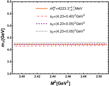
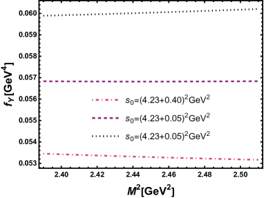
Figure 2: The mass [first] and the decay constant of $Y(4230)$ [second] as a function of the Borel parameter $M^{2}$ at different fixed values of $s_{0}$.

The $\psi$(4230) branching ratios from PDGZyla et al. (2020)shows that

$$\frac{\Gamma(J/\psi f_{0}(980),f_{0}(980)\to\pi^{+}\pi^{-})}{\Gamma(J/\psi\pi^{+}\pi^{-})}=0.17\pm 0.13.$$ (51)

We can estimate the upper limit of $\Gamma(J/\psi f_{0}(980)$, $f_{0}(980)\to\pi^{+}\pi^{-})$, by assuming that $\psi\to$ $J/\psi\pi^{+}\pi^{-}$ is the only decay process of $\psi(4230)$ With the width of $\Gamma_{\psi}=76.6\pm 14.2\pm 2.4$ MeV, we can obtain

$$\Gamma(\psi\to J/\psi f_{0}(980),f_{0}(980)\to\pi^{+}\pi^{-})=$$ (52)

$$\Gamma(\psi\to J/\psi f_{0}(980))\mathcal{B}(f_{0}(980)\to\pi^{+}\pi^{-})<13.022\ \text{MeV}.$$

Also from PDG one can find from the $f_{0}$(980) branching ratios that

$$\frac{\Gamma(\pi\pi)}{(\Gamma(\pi\pi)+\Gamma(K\bar{K}))}=0.75^{+0.11}_{-0.13},$$ (53)

and the partial width that

$$P(f_{0}(980)\to\gamma\gamma)\equiv\frac{\Gamma(f_{0}(980)\to\gamma\gamma)}{\Gamma(f_{0}(980))}=0.31^{+0.05}_{-0.04}.$$ (54)

The process $f_{0}(980)\to\pi\pi$, $f_{0}(980)\to K\bar{K}$ and $f_{0}(980)\to\gamma\gamma$ are the main decay process of $f_{0}$(980). From Eq.(54) comes out the partial width $P(f_{0}(980)\to\Gamma(\pi\pi)+\Gamma(K\bar{K}))=0.69^{+0.04}_{-0.05}$. So we estimate

$$\mathcal{B}(f_{0}(980)\to\pi^{+}\pi^{-})$$ (55)

$$\approx 0.75^{+0.11}_{-0.13}\times P(f_{0}(980)\to\Gamma(\pi\pi)+\Gamma(K\bar{K}))\approx 0.52.$$

Then we can finally conclude that

$$\Gamma(\psi\to J/\psi f_{0}(980))<25.0\ \text{MeV}.$$ (56)

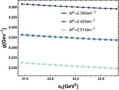
Figure 3: The strong coupling $g_{YJ/\psi f_{0}(980)}$ as a function of the threshold parameter $s_{0}$ at different fixed values of $M^{2}$

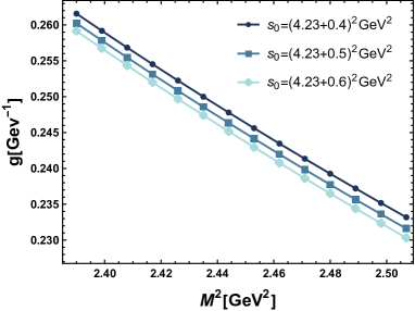
Figure 4: The strong coupling $g_{YJ/\psi f_{0}(980)}$ as a function of the Borel parameter $M^{2}$ at different fixed values of $s_{0}$

As we seen in Fig.4, the blue, green and black curves show clear dependence of our prediction on $s_{0}$ and $M^{2}$. For $M^{2}$ and $s_{0}$, we use the same values as in the analysis of the mass. The result is shown in Fig.3 and Fig.4. By choosing appropriate parameters, our prediction for $g_{YJ/\psi f_{0}}$ is

$$g_{YJ/\psi f_{0}}=(0.245\pm 0.01)\ \text{GeV}^{-1}.$$ (57)

Where we take the average result of $g_{YJ/\psi f_{0}}$. The width of this decay can be obtained by means of Eq.(32)

$$\Gamma(Y\rightarrow J/\psi f_{0}(980))=(1.28\pm 0.1)\ \text{MeV},$$ (58)

which is less than the upper limit of $\psi$(4230) $\to J/\psi f_{0}(980)$ decay width. Combining this result with the prediction result of mass, we may conclude that $Y$(4230) could be a tetraquark state. But, since the lack of experiments data about $\psi$(4230) $\to J/\psi f_{0}(980)$ decay width, we still need future experiments to further determine whether $Y$(4230) have the possibility be a tetraquark state or not.

IV Summary

In this research, we designate $Y$(4230) as a vector tetraquark state in order to concurrently analyze $Y(4230)$’s mass, decay constant, and decay into $J/\psi f_{0}(980)$. The mass of $Y(4230)$ is evaluated through a different calculation technique developed in two-point sum rules, and the result is in agreement with the mass of $Y(4230)$ in PDG. Then we extend the technique to calculate the decay constant of $Y(4230)$. Using the method of light cone sum rules, we calculate the coupling constant $g_{YJ/\psi f_{0}}$ and discover the result for $Y\to J/\psi f_{0}(980)$ decay width. Then we assume that $J/\psi\pi\pi$ is the most significant channel, overwhelming all the other channels. Therefore we can consider the width of $\psi(4230)$ as the width of $J/\psi\pi\pi$. Since we know the branching ratios of $\Gamma(J/\psi f_{0}(980),f_{0}(980)\to\pi^{+}\pi^{-})/\Gamma(J/\psi\pi^{+}\pi^{-})$from PDG, we can estimate the upper limit of $J/\psi f_{0}$ channel. The decay width of $Y\to J/\psi f_{0}(980)$ is less than the upper limit. Our prediction of the mass of $Y(4230)$ is in agreement with that of $Y(4230)$ in PDG and the decay width of $Y(4230)\to J/\psi f_{0}(980)$ does not exceed its theoretical limits. There is a possibility that $Y$(4230) could be a tetraquark. In the future, experiments will be more helpful in determining whether or not this structure of $Y(4230)$ is appropriate.

V Appendix

V.1 Particle distribution amplitudes

The matrix elements of the $f_{0}$ can be expanded in terms of the corresponding distribution amplitudes. Below we provide expressions for $\braket{f_{0}(980)(q)}{\bar{d}(x)\Gamma^{a}u(0)}{0}$Colangelo et al. (2010):

$$\braket{f_{0}(q)}{\bar{s}(x)\gamma_{\mu}s(0)}{0}=\bar{f}_{f_{0}}q_{\mu}\int_{0}^{1}due^{iuq\cdot x}\Phi_{f_{0}}(u),$$ (59)

$$\braket{f_{0}(q)}{\bar{s}(x)s(0)}{0}=m_{f_{0}}\bar{f}_{f_{0}}\int_{0}^{1}due^{iuq\cdot x}\Phi_{f_{0}}^{s}(u),$$

$$\braket{f_{0}(q)}{\bar{s}(x)\sigma_{\mu\nu}s(0)}{0}$$

$$=-\frac{m_{f_{0}}}{6}\bar{f}_{f_{0}}(q_{\mu}x_{\nu}-q_{\nu}x_{\mu})\int_{0}^{1}due^{iuq\cdot x}\Phi_{f_{0}}^{\sigma}(u),$$

where the LCDA $\Phi_{f_{0}}$ is twist-2 light-cone distribution amplitudes of $f_{0}(980)$, and the other two are twist-3 distribution amplitudes. Meantime, we use the following normalization

$$\int_{0}^{1}du\Phi_{f_{0}}(u)=0,\int_{0}^{1}du\Phi_{f_{0}}^{s}(u)=1,\int_{0}^{1}du\Phi_{f_{0}}^{\sigma}(u)=1.$$ (60)

V.2 The formula for LCSR

When calculate the OPE part of the correlation function, we will encounter various four-dimensional integrals in the momentum spaces. Before performing the integration, it is often to use the Feynman’s parametric integral formula:

$$\frac{1}{A_{1}^{a_{1}}\cdot\cdot\cdot A^{a_{n}}_{n}}=\frac{\Gamma(a_{1}\cdot\cdot\cdot a_{n})}{\Gamma(a_{1})\cdot\cdot\cdot\Gamma(a_{n})}\int_{0}^{1}dx_{1}\cdot\cdot\cdot\int_{0}^{1}dx_{n}$$ (61)

$$\frac{\delta(1-x_{1}+\cdot\cdot\cdot+x_{n})x_{1}^{a_{1}-1}\cdot x_{2}^{a_{2}-1}\cdot\cdot\cdot x_{n}^{a_{n}-1}}{(x_{1}A_{1}+\cdot\cdot\cdot+x_{n}A_{n})^{a_{1}+\cdot\cdot\cdot a_{n}}}.$$

In general, Feynman integrals contain:

$$I(D;a,q)=\int\frac{d^{D}p}{(2\pi)^{D}}\frac{1}{(p^{2}+2pq+m^{2})^{a}}.$$ (62)

This integral can be reduced to

$$I(D;a,q) =\int\frac{d^{D}p}{(2\pi)^{D}}\frac{1}{(p^{2}+2pq+m^{2})^{a}}$$ (63)

$$=\frac{1}{(4\pi)^{D/2}}\frac{\Gamma(a-D/2)}{\Gamma(a)}(m^{2}-q^{2})^{D/2-a}.$$

To obtain a formula in proportion to $p_{\mu}$ like

$$I(D;a,q) =\int\frac{d^{D}p}{(2\pi)^{D}}\frac{p_{\mu}}{(p^{2}+2pq+m^{2})^{a}}$$ (64)

$$=\frac{1}{(4\pi)^{D/2}}\frac{\Gamma(a-D/2)}{\Gamma(a)}\frac{q_{\mu}}{(m^{2}-q^{2})^{-D/2+a}},$$

we can differentiate equation Eq.(62) with momentum $q$ one time. The higher tensors $p_{\mu}\cdots p_{\nu}$ in the integrand come form higher differentiations. Now above equation encounter a pole in Gamma function when dimension $D\to 4$, i.e. $\Gamma(0)\to\infty$. We can use equation

$$\frac{\Gamma(n-\frac{1}{2}d)}{a^{2n-d}}=\int_{0}^{\infty}d\lambda\lambda^{n-d/2-1}e^{-\lambda a^{2}}$$ (65)

to get rid of Gamma function and perform the replacement

$$\int_{0}^{\infty}\frac{d\lambda}{\lambda^{n}}e^{-\lambda K}\to(-1)^{n}\frac{K^{n-1}lnK}{(n-1)!}.$$ (66)

To obtain the final expression of the correlation function, we need the imaginary part of results and the integration over the Feynman parameters.

V.3 The formula for mass and decay constants

Here we present calculation details of integral when we dealing with Eq.(7). we need to consider a general integral

$$I(p^{2})=\int d^{4}xe^{ipx}\frac{1}{(x^{2})^{n}}\frac{K_{i}(m_{1}\sqrt{-x^{2}})}{(\sqrt{-x^{2}})^{i}}\frac{K_{j}(m_{2}\sqrt{-x^{2}})}{(\sqrt{-x^{2}})^{j}}.$$ (67)

Use the integral representation of Bessel function

$$\frac{K_{i}(m_{1}\sqrt{-x^{2}})}{(\sqrt{-x^{2}})^{i}}=\int_{0}^{\infty}\frac{dt}{t^{i+1}}\exp{[-\frac{m_{1}}{2}(t-\frac{x^{2}}{t})]},$$ (68)

we have

$$I= \frac{1}{4}\int d^{4}xe^{ipx}\frac{1}{(x^{2})^{n}}\int_{0}^{\infty}\frac{dt_{1}}{t_{1}^{i+1}}\exp{[-\frac{m_{1}}{2}(t_{1}-\frac{x^{2}}{t_{1}})]}$$ (69)

$$\times\int_{0}^{\infty}\frac{dt_{2}}{t_{2}^{j+1}}\exp{[-\frac{m_{2}}{2}(t_{2}-\frac{x^{2}}{t_{2}})]}$$

$$= \frac{i(-1)^{n}}{4\Gamma(n)}\int d^{4}xe^{ipx}\int_{0}^{\infty}d\lambda\lambda^{n-1}\exp(-\lambda x^{2})\int_{0}^{\infty}\frac{dt_{1}}{t_{1}^{i+1}}$$

$$\times\exp{[-\frac{m_{1}}{2}(t_{1}+\frac{x^{2}}{t_{1}})]}\int_{0}^{\infty}\frac{dt_{2}}{t_{2}^{j+1}}\exp{[-\frac{m_{2}}{2}(t_{2}+\frac{x^{2}}{t_{2}})]}.$$

Introduce new variables

$$a=\frac{2m_{1}}{t_{1}},\ b=\frac{2m_{2}}{t_{2}}\to dt_{1}=-\frac{2m_{1}}{a^{2}}da,\ dt_{2}=-\frac{2m_{2}}{b^{2}}db,$$ (70)

leading to equation

$$I =\frac{(-1)^{n}i}{4\Gamma(n)}\frac{1}{(2m_{1})^{i}(2m_{2})^{j}}\int_{0}^{\infty}da\ a^{i-1}\int_{0}^{\infty}db\ b^{j-1}\int_{0}^{\infty}d\lambda\lambda^{n-1}$$ (71)

$$\times\exp[-(\frac{m_{1}^{2}}{a}+\frac{m_{2}^{2}}{b})]\int d^{4}x\ \exp{[-\frac{1}{4}(a+b+4\lambda)x^{2}-ipx]}$$

$$=\frac{(-1)^{n}i}{4\Gamma(n)}\frac{16\pi^{2}}{(2m_{1})^{i}(2m_{2})^{j}}\int_{0}^{\infty}da\int_{0}^{\infty}db\ a^{i-1}b^{j-1}\int_{0}^{\infty}d\lambda\lambda^{n-1}$$

$$\times\frac{1}{(a+b+4\lambda)^{2}}\exp[\frac{-p^{2}}{(a+b+4\lambda)}]\exp[-(\frac{m_{1}^{2}}{a}+\frac{m_{2}^{2}}{b})].$$

Than perform $a\to 4a$, $b\to 4b$, we obtain

$$I= \frac{(-1)^{n}i}{\Gamma(n)}\frac{2^{i+j-2}\pi^{2}}{(m_{1})^{i}(m_{2})^{j}}\int_{0}^{\infty}da\int_{0}^{\infty}db\ a^{i-1}b^{j-1}\int_{0}^{\infty}d\lambda\lambda^{n-1}$$ (72)

$$\times\frac{1}{(a+b+\lambda)^{2}}\exp[\frac{-p^{2}}{4(a+b+\lambda)}]\exp[-(\frac{m_{1}^{2}}{4a}+\frac{m_{2}^{2}}{4b})].$$

Now we introduce the variables $\rho$, $x$, and $y$, defined by

$$\rho=(a+b+\lambda),x=\frac{a}{a+b+\lambda},y=\frac{b}{a+b+\lambda}.$$ (73)

Then we have

$$\mbox{d}\lambda\mbox{d}a\mbox{d}b =\begin{vmatrix}\frac{\partial\lambda}{\partial\rho}&\frac{\partial a}{\partial x}&\frac{\partial b}{\partial y}\\ \frac{\partial\lambda}{\partial\rho}&\frac{\partial a}{\partial x}&\frac{\partial b}{\partial y}\\ \frac{\partial\lambda}{\partial\rho}&\frac{\partial a}{\partial x}&\frac{\partial b}{\partial y}\end{vmatrix}\mbox{d}\rho\mbox{d}x\mbox{d}y$$ (74)

$$=\rho^{2}\mbox{d}\rho\mbox{d}x\mbox{d}y,$$

which leads to

$$I=\frac{(-1)^{n}i}{\Gamma(n)}\frac{2^{i+j-2}\pi^{2}}{(m_{1})^{i}(m_{2})^{j}}\int du\varphi(u)\int_{0}^{\infty}d\rho\int_{0}^{1}dx\int_{0}^{1}dy(\rho x)^{i-1}$$ (75)

$$\times(\rho y)^{j-1}(\rho(1-x-y))^{n-1}\exp[\frac{-p^{2}}{4\rho}]\exp[-(\frac{m_{1}^{2}}{4\rho x}+\frac{m_{2}^{2}}{4\rho y})].$$

Applying the double Borel transformations with respect to $-p^{2}\to M^{2}$, we obtain

$$\tilde{I}(M^{2})=\frac{(-1)^{n}i}{\Gamma(n)}\frac{2^{i+j-2}\pi^{2}}{(m_{1})^{i}(m_{2})^{j}}\int_{0}^{\infty}d\rho\int_{0}^{1}dx\int_{0}^{1}dy(\rho x)^{i-1}$$ (76)

$$\times(\rho y)^{j-1}(\rho(1-x-y))^{n-1}\delta(\frac{1}{M^{2}}-\frac{1}{4\rho})\exp[-(\frac{m_{1}^{2}}{4\rho x}+\frac{m_{2}^{2}}{4\rho y})]$$

$$=\frac{(-1)^{n}i}{\Gamma(n)}\frac{2^{2-2n-i-j}\pi^{2}}{(m_{1})^{i}(m_{2})^{j}}(M^{2})^{i+j+n-1}\int_{0}^{1}dx\int_{0}^{1}dy$$

$$\times x^{i-1}y^{j-1}(1-x-y)^{n-1}\exp[-(\frac{m_{1}^{2}}{M^{2}x}+\frac{m_{2}^{2}}{M^{2}y})],$$

where $\rho_{0}=\frac{M^{2}}{4}$.

Introducing new variables, $\sigma_{i}=\frac{1}{M_{i}^{2}}$, we have

$$\tilde{I}(\sigma) =\frac{(-1)^{n}i}{\Gamma(n)}\frac{2^{2-2n-i-j}\pi^{2}}{(m_{1})^{i}(m_{2})^{j}}\frac{1}{\sigma^{i+j+n-1}}\int_{0}^{1}dx\int_{0}^{1}dy$$ (77)

$$\times x^{i-1}y^{j-1}(1-x-y)^{n-1}\exp[-(\frac{m_{1}^{2}}{x}+\frac{m_{2}^{2}}{y})\sigma]$$

$$=\frac{C}{\Gamma(i+j+n-1)}\int_{0}^{1}dx\int_{0}^{1}dyx^{i-1}y^{j-1}(1-x-y)^{n-1}$$

$$\times\exp[-(\frac{m_{1}^{2}}{x}+\frac{m_{2}^{2}}{y})\sigma]\int_{0}^{\infty}\mbox{d}z\exp[-z\sigma]z^{i+j+n-2}$$

$$=\frac{C}{\Gamma(i+j+n-1)}\int_{0}^{1}dx\int_{0}^{1}dyx^{i-1}y^{j-1}(1-x-y)^{n-1}$$

$$\times\int_{0}^{\infty}\mbox{d}z\exp[-(z+\frac{m_{1}^{2}}{x}+\frac{m_{2}^{2}}{y})\sigma]z^{i+j+n-2}.$$

Where $C=\frac{(-1)^{n}i}{\Gamma(n)}\frac{2^{2-2n-i-j}\pi^{2}}{(m_{1})^{i}(m_{2})^{j}}$. Applying double Borel transformation with respect to $\sigma\to\frac{1}{s}$, we obtain the spectral density

$$\rho(s) =\frac{C}{\Gamma(i+j+n-1)}\int_{0}^{1}dx\int_{0}^{1}dyx^{i-1}y^{j-1}(1-x-y)^{n-1}$$ (78)

$$\times\int_{0}^{\infty}\mbox{d}z\delta[s-(z+\frac{m_{1}^{2}}{x}+\frac{m_{2}^{2}}{y})]z^{i+j+n-2}$$

$$=\frac{C}{\Gamma(i+j+n-1)}\int_{0}^{1}dx\int_{0}^{1}dyx^{i-1}y^{j-1}(1-x-y)^{n-1}$$

$$\times(s-\frac{m_{1}^{2}}{x}-\frac{m_{2}^{2}}{y})^{i+j+n-2}\theta(s-\frac{m_{1}^{2}}{x}-\frac{m_{2}^{2}}{y}).$$

Similarly, we also need to consider integral

$$I =\int d^{4}xe^{ipx}\frac{x^{\mu}x^{\nu}}{(x^{2})^{n}}\frac{K_{i}(m_{1}\sqrt{-x^{2}})}{(\sqrt{-x^{2}})^{i}}\frac{K_{j}(m_{2}\sqrt{-x^{2}})}{(\sqrt{-x^{2}})^{j}}$$ (79)

$$=-\partial_{\mu}^{(p)}\partial_{\nu}^{(p)}\int d^{4}xe^{ipx}\frac{1}{(x^{2})^{n}}\frac{K_{i}(m_{1}\sqrt{-x^{2}})}{(\sqrt{-x^{2}})^{i}}\frac{K_{j}(m_{2}\sqrt{-x^{2}})}{(\sqrt{-x^{2}})^{j}},$$

and derived spectral density

$$\rho(s) =\frac{C_{1}}{\Gamma(i+j+n+1)}\int_{0}^{1}dx\int_{0}^{1}dyx^{i-1}y^{j-1}(1-x-y)^{n-1}$$ (80)

$$\times(s-\frac{m_{1}^{2}}{x}-\frac{m_{2}^{2}}{y})^{i+j+n}\theta(s-\frac{m_{1}^{2}}{x}-\frac{m_{2}^{2}}{y})p_{\mu}p_{\nu}$$

$$+\frac{C_{2}}{\Gamma(i+j+n)}\int_{0}^{1}dx\int_{0}^{1}dyx^{i-1}y^{j-1}(1-x-y)^{n-1}$$

$$\times(s-\frac{m_{1}^{2}}{x}+\frac{m_{2}^{2}}{y})^{i+j+n-1}\theta(s-\frac{m_{1}^{2}}{x}-\frac{m_{2}^{2}}{y})g_{\mu\nu},$$

Where $C_{1}=\frac{(-1)^{n+1}i}{\Gamma(n)}\frac{2^{4-2n-i-j}\pi^{2}}{(m_{1})^{i}(m_{2})^{j}}$, $C_{2}=\frac{(-1)^{n+2}i}{\Gamma(n)}\frac{2^{3-2n-i-j}\pi^{2}}{(m_{1})^{i}(m_{2})^{j}}$.