MLE-based Device Activity Detection under Rician Fading for Massive Grant-free Access with Perfect and Imperfect Synchronization

Abstract

Most existing studies on massive grant-free access, proposed to support massive machine-type communications (mMTC) for the Internet of things (IoT), assume Rayleigh fading and perfect synchronization for simplicity. However, in practice, line-of-sight (LoS) components generally exist, and time and frequency synchronization are usually imperfect. This paper systematically investigates maximum likelihood estimation (MLE)-based device activity detection under Rician fading for massive grant-free access with perfect and imperfect synchronization. We assume that the large-scale fading powers, Rician factors, and normalized LoS components can be estimated offline. We formulate device activity detection in the synchronous case and joint device activity and offset detection in three asynchronous cases (i.e., time, frequency, and time and frequency asynchronous cases) as MLE problems. In the synchronous case, we propose an iterative algorithm to obtain a stationary point of the MLE problem. In each asynchronous case, we propose two iterative algorithms with identical detection performance but different computational complexities. In particular, one is computationally efficient for small ranges of offsets, whereas the other one, relying on fast Fourier transform (FFT) and inverse FFT, is computationally efficient for large ranges of offsets. The proposed algorithms generalize the existing MLE-based methods for Rayleigh fading and perfect synchronization. Numerical results show that the proposed algorithm for the synchronous case can reduce the detection error probability by up to $50.4\%$ at a $78.6\%$ computation time increase, compared to the MLE-based state-of-the-art, and the proposed algorithms for the three asynchronous cases can reduce the detection error probabilities and computation times by up to $65.8\%$ and $92.0\%$, respectively, compared to the MLE-based state-of-the-arts.

I Introduction

Massive machine-type communications (mMTC), one of the three generic services in the fifth generation (5G) wireless networks, are expected to provide massive connectivity to a vast number of Internet-of-Things (IoT) devices [2, 3]. The fundamental challenge of mMTC is to enable efficient and timely data transmission from enormous IoT devices that are cheap, energy-limited, and sporadically active with small packets to send. Conventional grant-based access is no longer suitable for mMTC, as the handshaking procedure for obtaining a grant results in excessive control signaling cost and high transmission latency. Recently, grant-free access, whose goal is to let devices transmit data in an arrive-and-go manner without waiting for the base station (BS) to schedule a grant, has been identified by the Third Generation Partnership Project (3GPP) as a promising solution to support mMTC [4].

This paper focuses on a widely investigated grant-free access scheme consisting of a pilot transmission phase and a data transmission phase [3]. Specifically, devices within a cell are preassigned non-orthogonal pilot sequences that are known to the BS. In the pilot transmission phase, active devices send their pilots to the BS simultaneously, and the BS detects the activity states of all devices and estimates the channel states of the active devices from the received pilot signals. In the data transmission phase, all active devices transmit their data to the BS, and the BS detects their transmitted data from the received data signals based on the channels obtained in the pilot transmission phase. The device activity detection and channel estimation at the BS are essential for realizing grant-free access.

A Related works

Existing works on device activity detection and channel estimation mainly rely on compressed sensing (CS), statistical estimation, and machine learning techniques. Most works [5, 6, 7, 8, 9, 10, 11, 12, 13, 14] study only the pilot phase and focus on activity detection and channel estimation. For instance, [5, 6, 11] solve device activity detection and channel estimation problems using CS techniques, such as approximate message passing (AMP) [5] and group least absolute shrinkage and selection operator (LASSO) [6, 11]. The AMP-based algorithms are computationally efficient but the activity detection and channel estimation accuracies degrade significantly if the number of active devices is larger than the pilot length [7]. Besides, leveraging statistical estimation techniques, [7, 8, 9, 10] formulate device activity detection as maximum likelihood estimation (MLE) problems [7, 8, 9] and maximum a posterior probability estimation (MAPE) problems [9, 10] under flat [7, 8, 9] and frequency selective [10] Rayleigh fading and tackle the non-convex problems using the coordinate descent (CD) method. The statistical estimation approaches generally outperform the CS-based approaches in activity detection accuracy at the cost of computation complexity increase [7] and have fewer restrictions on the system parameters. Recently, [11, 12, 13, 14] tackle device activity detection and channel estimation using MAPE-based [11], group LASSO-based [11, 13], and AMP-based [11, 14] model-driven neural networks and data-driven neural networks [12]. The machine learning techniques are computational efficient but have no performance guarantee. Some works [15, 16] consider pilot and data phases and jointly design activity detection, channel estimation, and data detection. For instance, [15] and [16] solve the joint activity, channel, and data estimation problems using bilinear generalized approximate message passing (BiGAMP). Note that the BiGAMP-based algorithms [15, 16] outperform the AMP-based algorithms in activity detection and channel estimation accuracies at the cost of computation complexity increase. On the other hand, some works [17, 18] study grant-free access scheme with data-embedding pilots. Specifically, there is one phase where each device sends one of its pre-assigned data-embedding pilots, and the BS jointly detects device activity and sent data. For instance, [17, 18] formulate joint device activity and data detection as MLE problems and tackle the non-convex problems using the CD method [17] and projected gradient method [18]. These approaches [17, 18] are suitable only for very small data payloads as their computational complexities significantly increase with the number of information bits embedded in pilots (or pre-assigned data-embedding pilots per device).

The works mentioned above [5, 6, 11, 7, 8, 17, 9, 13, 14, 10, 15, 16, 18] assume that all active devices send their pilots synchronously in time and frequency, referred to as the synchronous case in this paper. In practice, time synchronization and frequency synchronization are usually imperfect for low-cost IoT devices, due to the lack of coordination between the BS and IoT devices and frequency drifts of cheap crystal oscillators equipped by IoT devices, respectively [19, 20]. If not appropriately handled, the presence of symbol time offsets (STOs) and/or carrier frequency offsets (CFOs) may severely deteriorate the performance of device activity detection and channel estimation. In the asynchronous cases, the BS has to estimate the unknown activities and channel states together with the unknown offsets of all devices from the same number of observations as in the synchronous case. Besides, the offset of each device lies in a much larger set than the activity state of each device. Thus, the device activity detection and channel estimation in the asynchronous cases are more challenging than those in the synchronous case. Some recent works primarily investigate the time and/or frequency asynchronous cases and attempt to address this challenge. For instance, [21, 22, 23] investigate joint device activity detection and channel estimation in the time asynchronous case using an AMP-based model-driven neural network [21], group LASSO [22], and an MLE-based method [23], respectively. For the frequency asynchronous case, [24] deals with joint device activity detection and channel estimation using norm approximation, and [25] and [26] handle device activity detection using MLE-based methods. For the time and frequency asynchronous case, [27] investigates joint device activity detection and channel estimation for an orthogonal frequency division multiplexing (OFDM) system using an AMP-based method. The optimization problems in [23, 22, 24, 25, 26] are solved using the majorization-minimization method [24], CD method [25], and block coordinate descent (BCD) method [22, 23, 26]. Notice that most existing works [22, 25, 24, 27] incur much higher computational complexities than those for the synchronous case, as the dominant terms of their computation costs significantly increase with the offset range. When the offset range is large, their computational complexities are exceedingly high and may not be practical. To address this issue, our early work [26] proposes a low-complexity algorithm, whose computation cost (dominant term) does not change with the CFO range, to solve the MLE problem for the frequency asynchronous case under Rayleigh fading using the BCD method and fast Fourier transform (FFT).

Most existing studies on massive grant-free access that utilize channel statistics to improve estimation performance assume Rayleigh fading for simplicity [5, 26, 11, 7, 8, 17, 9, 13, 14, 25, 27, 21, 10, 18]. However, channel measurement results have shown that line-of-sight (LoS) components always exist in sub-6 GHz and millimeter wave bands [28, 29]. Hence, Rician fading (including both LoS components and non-line-of-sight (NLoS) components) includes Rayleigh fading (with only NLoS components) as a special case and can be applied to a wider variety of wireless communications systems than Rayleigh fading. Although device activity detection and channel estimation methods proposed for Rayleigh fading in [7, 9, 8, 23, 26] can be applied to Rician fading in a brute force manner, the resulting performance may significantly degrade. Under Rician fading, the means of the channel states of devices are non-zero and can be significantly different, unlike under Rayleigh fading, where the means of the channel states of devices are zero. Thus, due to more complex channel statistics, device activity detection and channel estimation under Rician fading are more challenging than those under Rayleigh fading. In [30], the authors attempt to solve the MLE-based device activity detection problem for the synchronous case under Rician fading with known Rician factors and LoS components. Nevertheless, the two-loop iterative algorithm proposed in [30] is not computationally efficient, solves only an approximation of the block coordinate optimization problem, and cannot guarantee to obtain a stationary point. Note that massive grant-free access for the asynchronous cases under Rician fading has not been investigated yet. In summary, detecting device activities under Rician fading for massive grant-free access with perfect and imperfect synchronization remains an open problem.

B Contributions

In this paper, we would like to shed some light on this problem. In particular, we investigate MLE-based device activity detection under Rician fading with known large-scale fading powers, Rician factors, and normalized LoS components for the synchronous case and three asynchronous cases, i.e., time asynchronous case, frequency asynchronous case, and time and frequency asynchronous case. The main contributions of this paper are listed as follows.

• In the synchronous case, we formulate device activity detection under Rician fading as an MLE problem, which is non-convex with a complicated objective function. Unlike the MLE problem for Rayleigh fading [7, 8], the challenge of dealing with the MLE problem for Rician fading lies in how to effectively and efficiently handle the term in the objective function that is related to the LoS components. Based on the BCD method, we develop an iterative algorithm (Prop-MLE-Syn), where all block coordinate optimization problems are solved analytically to obtain a stationary point of the MLE problem. Note that the proposed method successfully generalizes the MLE-based method for Rayleigh fading in the synchronous case [8].

• In each of the three asynchronous cases, we formulate joint device activity and offset detection under Rician fading as an MLE problem, which is more challenging than the one in the synchronous case. Based on the BCD method, we develop two iterative algorithms where all block coordinate optimization problems are solved analytically to tackle the MLE problem. Note that the two iterative algorithms have identical detection performance but different computational complexities and are suitable for different ranges of offset values. In particular, one (referred to as Prop-MLE-Small) is computationally efficient for a small range of offset values, whereas the other one (referred to as Prop-MLE-Large), relying on FFT and inverse fast Fourier transform (IFFT), is computationally efficient for a large range of offset values. We also analytically compare the computational complexities of the two iterative algorithms. Note that the proposed algorithms successfully generalize the MLE-based methods for Rayleigh fading in the time asynchronous case [23] and frequency asynchronous case [26].

Numerical results show that the proposed algorithm for the synchronous case can reduce the detection error probability by up to $50.4\%$ at a $78.6\%$ computation time increase, compared to the MLE-based state-of-the-art, and the proposed algorithms for the three asynchronous cases can reduce the detection error probabilities and computation times by up to $65.8\%$ and $92.0\%$, respectively, compared to the MLE-based state-of–the-arts. To our knowledge, this is the first work that utilizes FFT and IFFT techniques to accelerate device activity detection algorithms for massive grant-free access with general imperfect synchronization. Besides, this is the first work that provides systematic MLE-based device activity detection methods under Rician fading for massive grant-free access with general imperfect synchronization. The abbreviations in this paper are listed in Table I.

TABLE I: Abbreviation

mMTC	massive machine-type communications	(B)CD	(block) coordinate descent
5G	the fifth generation	MAPE	maximum a posterior probability estimation
IoT	Internet-of-Things	STO	symbol time offset
BS	base station	CFO	carrier frequency offset
3GPP	the Third Generation Partnership Project	OFDM	orthogonal frequency division multiplexing
CS	compressed sensing	(N)LoS	(non)-line-of-sight
AMP	approximate message passing	(I)FFT	(inverse) fast Fourier transform
LASSO	least absolute shrinkage and selection operator	(I)DFT	(inverse) discrete Fourier
BiGAMP	bilinear generalized approximate message passing	i.i.d.	independent and identically distributed
MLE	maximum likelihood estimation	p.d.f.	probability density function
AWGN	the additive white Gaussian noise

Notation

In this paper, unless otherwise stated, we represent scalar constants by non-boldface letters (e.g., $x$ or $X$), vectors by boldface small letters (e.g., $\mathbf{x}$), matrices by boldface capital letters (e.g., $\mathbf{X}$), and sets by calligraphic letters (e.g., $\mathcal{X}$). $\mathbf{X}^{H}$, $\mathbf{X}^{T}$, $\mathbf{X}^{*}$, and $\mathrm{tr}(\mathbf{X})$ denote the transpose conjugate, transpose, conjugation, and trace of matrix $\mathbf{X}$, respectively. For $\mathcal{A}=\{a_{1},a_{2},...,a_{N}\}$ where $a_{1}<\cdots<a_{N}$ and $\mathcal{B}=\{b_{1},b_{2},...,b_{M}\}$ where $b_{1}<\cdots<b_{M}$, the notations $(x_{a})_{a\in\mathcal{A}}$, $(\mathbf{x}_{b})_{b\in\mathcal{B}}$, and $(x_{a,b})_{a\in\mathcal{A},b\in\mathcal{B}}$ represent vector $[x_{a_{1}},x_{a_{2}},...,x_{a_{N}}]^{T}$, matrix $[\mathbf{x}_{b_{1}},\mathbf{x}_{b_{2}},...,\mathbf{x}_{b_{M}}]$, and a matrix whose $(n,m)$-th element is $x_{a_{n},b_{m}}$, respectively. The notations $(\mathbf{x})_{n}$ and $(\mathbf{x})_{\mathcal{A}}$ denote the $n$-th element of vector $\mathbf{x}$ and a column vector consisting of elements of vector $\mathbf{x}$ indexed by $\mathcal{A}$, respectively, $(\mathbf{X})_{n,m}$ denotes the $(n,m)$-th element of matrix $\mathbf{X}$, $\mathbf{X}_{n,:}$ and $\mathbf{X}_{:,m}$ denote the $n$-th row and the $m$-th column of matrix $\mathbf{X}$, respectively, and $\mathbf{X}_{\mathcal{A},:}$ and $\mathbf{X}_{:,\mathcal{B}}$ denote matrices consisting of rows of matrix $\mathbf{X}$ indexed by $\mathcal{A}$ and columns of matrix $\mathbf{X}$ indexed by $\mathcal{B}$, respectively. The complex field, real field, positive real field, and positive integer field are denoted by $\mathbb{C}$, $\mathbb{R}$, $\mathbb{R}^{+}$, and $\mathbb{N}^{+}$, respectively. The notations $\mathbf{F}_{K}\triangleq(e^{-j\frac{2\pi}{K}(n-1)(m-1)})_{n,m\in\{1,2,...,K\}}$ and $\frac{1}{K}\mathbf{F}_{K}^{H}$ denote the $K$-dimensional discrete Fourier transform (DFT) and inverse discrete Fourier transform (IDFT) matrices, respectively, and $\mathrm{FFT}(\mathbf{x})\triangleq\mathbf{F}_{K}\mathbf{x}$ and $\mathrm{IFFT}(\mathbf{x})\triangleq\frac{1}{K}\mathbf{F}_{K}^{H}\mathbf{x}$ represent the FFT and IFFT of vector $\mathbf{x}\in\mathbb{C}^{K}$, respectively. The notation $\mathrm{diag}(\mathbf{x})$ represents the diagonal matrix with diagonal elements $\mathbf{x}$, $\mathrm{Re}(\cdot)$ denotes the real part of a scalar, a vector, or a matrix, $\log(\cdot)$ and $\log_{2}(\cdot)$ denote the logarithms for base $e$ and base $2$, respectively, $\odot$ represents the element-wise product of matrices of the same size, $\mathbb{I}(\cdot)$ denotes the indicator function, and $\mathbf{I}_{K}$, $\mathbf{1}_{K}$, and $\mathbf{0}_{K}$ denote the $K$-dimensional identity matrix, all-one vector, and zero vector, respectively.

II System Model

We consider the uplink of a single-cell wireless network consisting of one $M$-antenna BS and $N$ single-antenna IoT devices. Let $\mathcal{M}\triangleq\{1,2,...,M\}$ and $\mathcal{N}\triangleq\{1,2,...,N\}$ denote the sets of antennas and device indices, respectively. The locations of the BS and devices are assumed to be fixed. As many other papers [5, 6, 11, 7, 24, 8, 25, 17, 9, 13, 14, 10, 15, 16, 18, 21, 22, 23, 26, 30], we consider a narrow-band system, assume slow fading, and adopt the block fading model for slow fading. We study one resource block within the coherence time. Let $\sqrt{g_{n}}{\bf h}_{n}\in{\mathbb{C}}^{M}$ denote the channel vector between device $n$ and the BS in the coherence block, where $g_{n}\in\mathbb{R}^{+}$ represents the large-scale fading power, and $\mathbf{h}_{n}\triangleq(h_{n,m})_{m\in\mathcal{M}}\in{\mathbb{C}}^{M}$ denotes the small-scale fading coefficients, where $h_{n,m}$ denotes the small-scale fading coefficient between the BS’s $m$-th antenna and device $n$. Denote the large scale-fading power vector by $\mathbf{g}\triangleq(g_{n})_{n\in\mathcal{N}}\in\mathbb{R}^{N}$. In contrast to most existing works which consider Rayleigh fading [5, 11, 7, 8, 17, 9, 13, 14, 25, 27, 21, 10, 26, 18], we consider the Rician small-scale fading model for $\mathbf{h}_{n}$, $n\in\mathcal{N}$. Note that the Rician fading model generalizes the Rayleigh fading model and can capture the LoS components when devices are located in open outdoor or far from the ground. Specifically,

$$\mathbf{h}_{n}=\sqrt{\frac{\kappa_{n}}{1+\kappa_{n}}}\overline{\mathbf{h}}_{n}+\sqrt{\frac{1}{1+\kappa_{n}}}\widetilde{\mathbf{h}}_{n},\ n\in\mathcal{N},$$ (1)

where $\kappa_{n}>0$ denotes the Rician factor, $\overline{\mathbf{h}}_{n}\triangleq(\overline{h}_{n,m})_{m\in\mathcal{M}}\in{\mathbb{C}}^{M}$ represents the normalized LoS components with unit-modulus elements (i.e., $|\overline{h}_{n,m}|=1$, $m\in\mathcal{M}$), and $\widetilde{\mathbf{h}}_{n}\triangleq(\widetilde{h}_{n,m})_{m\in\mathcal{M}}\in{\mathbb{C}}^{M}$ represents the normalized NLoS components with elements independent and identically distributed (i.i.d.) according to $\mathcal{CN}(0,1)$. Thus, $h_{n,m}\sim\mathcal{CN}(\sqrt{\frac{\kappa_{n}}{1+\kappa_{n}}}\overline{h}_{n,m},\frac{1}{1+\kappa_{n}})$ for all $n\in\mathcal{N}$ and $m\in\mathcal{M}$. Let $\boldsymbol{\kappa}\triangleq(\kappa_{n})_{n\in\mathcal{N}}\in\mathbb{R}^{N}$ denote the Rician factor vector, and let $\overline{\mathbf{H}}\triangleq(\overline{\mathbf{h}}_{n})_{n\in\mathcal{N}}\in\mathbb{C}^{M\times N}$, $\widetilde{\mathbf{H}}\triangleq(\widetilde{\mathbf{h}}_{n})_{n\in\mathcal{N}}\in\mathbb{C}^{M\times N}$, and ${\mathbf{H}}\triangleq({\mathbf{h}}_{n})_{n\in\mathcal{N}}\in\mathbb{C}^{M\times N}$ denote the normalized LoS channel matrix, normalized NLoS channel matrix, and normalized channel matrix, respectively. We assume that $\mathbf{g}$, $\boldsymbol{\kappa}$, and $\overline{\mathbf{H}}$ are known constants, since they are dominantly determined by the distances and communication environment between the devices and the BS and can be estimated offline (e.g., in the deployment phase or once the communication environment changes significantly) if the locations of devices are fixed.

We study the massive access scenario arising from mMTC, where very few devices among a large number of potential devices are active and access the BS in each coherence block. For all $n\in\mathcal{N}$, let $a_{n}\in\{0,1\}$ denote the activity state of device $n$, where $a_{n}=1$ indicates that device $n$ is active, and $a_{n}=0$ otherwise. Denote the device activity vector by $\mathbf{a}\triangleq(a_{n})_{n\in\mathcal{N}}$. We adopt a grant-free access scheme [5, 6, 7, 8, 9, 10, 11, 13, 14]. Specifically, each device $n$ is pre-assigned a specific pilot sequence ${\bf p}_{n}\in{\mathbb{C}}^{L}$ consisting of $L$ ($L\ll N$) pilot symbols. In the pilot transmission phase, active devices send their length-$L$ pilots to the BS, and the BS detects the activity states of all devices and estimates the channel states of the active devices from the received pilot symbols over the $M$ antennas. In the data transmission phase, all active devices transmit their data to the BS, and the BS detects their transmitted data from the received data symbols based on the channels obtained in the pilot transmission phase. In this paper, we study the pilot transmission phase and investigate device activity detection, which is a fundamental problem for massive grant-free access [8, 7, 9].

Ideally, all active devices send their pilots and data synchronously in time and frequency, i.e., with the same reception time and carrier frequency. Nevertheless, time synchronization and frequency synchronization are usually imperfect. As such, the accuracy of a device activity detection scheme designed for the ideal time and frequency synchronous case may drop significantly. In this paper, we assume that the device activities are deterministic and unknown and investigate device activity detection under Rician fading in the pilot phase of synchronous and asynchronous cases. For ease of illustration, in the rest of this paper, we define $\mathbf{a}_{-n}\triangleq(a_{\ell})_{\ell\in\mathcal{N},\ell\neq n}$ and rewrite $\mathbf{a}$ as $(\mathbf{a}_{-n},a_{n})$, for all $n\in\mathcal{N}$.

A Synchronous Case

In the synchronous case, all active devices send their length-$L$ pilot sequences synchronously in time and frequency. Thus, this case is also referred to as the time and frequency synchronous case. Let $\mathbf{Y}\in\mathbb{C}^{L\times M}$ denote the received signal over $L$ signal dimensions and $M$ antennas at the BS. Then, we have:

$${\mathbf{Y}} =\sum\limits_{n\in\mathcal{N}}a_{n}\sqrt{g_{n}}\mathbf{p}_{n}\mathbf{h}_{n}^{T}+\mathbf{Z}$$

$$={\mathbf{P}}\mathbf{A}{\mathbf{\Gamma}}^{\frac{1}{2}}(\mathbf{K}^{\frac{1}{2}}\overline{\bf H}^{T}+\widetilde{\bf H}^{T})+{\bf Z},$$ (2)

where the last equality is due to (1). Here, $\mathbf{P}\triangleq(\mathbf{p}_{n})_{n\in\mathcal{N}}\in\mathbb{C}^{{L\times N}}$ represents the pre-assigned pilot matrix, ${\bf A}\triangleq\mathrm{diag}({\bf a})\in\mathbb{R}^{N\times N}$ is the diagonal matrix with diagonal elements $\mathbf{a}$, $\mathbf{\Gamma}\triangleq\mathrm{diag}\Big{(}\big{(}\frac{g_{n}}{1+\kappa_{n}}\big{)}_{n\in\mathcal{N}}\Big{)}\in\mathbb{R}^{N\times N}$ is the diagonal matrix with diagonal elements $\frac{g_{n}}{1+\kappa_{n}}$, $n\in\mathcal{N}$, $\mathbf{K}\triangleq\mathrm{diag}\left(\boldsymbol{\kappa}\right)\in\mathbb{R}^{N\times N}$ is the diagonal matrix with diagonal elements $\boldsymbol{\kappa}$, and ${\bf Z}\in\mathbb{C}^{L\times M}$ is the additive white Gaussian noise (AWGN) at the BS with all elements i.i.d. according to $\mathcal{CN}(0,\sigma^{2})$. In the synchronous case, the BS detects $\bf a$ from ${\bf Y}$ given in (2), based on the values of $\mathbf{P}$, $\mathbf{g}$, $\mathbf{K}$, $\overline{\mathbf{H}}$, and the distributions of $\mathbf{Z}$ and $\widetilde{\mathbf{H}}$.

B Asynchronous Cases

Following the convention [21, 22, 23], we assume that pilot signals sent by the devices are symbol synchronous for tractability, i.e., the time delays of pilot signals are multiples of the symbol duration. Consequently, let $t_{n}\in\mathcal{D}\triangleq\{0,1,...,D\}$ represent the STO for the pilot signal of device $n\in\mathcal{N}$, where $D\in\mathbb{N}^{+}$ denotes the maximum STO. Let $\omega_{n}\in[-\Omega,\Omega]$ denote the accumulated phase shift in one symbol duration, also called CFO [24, 25], where $\Omega\in[0,\pi]$ denotes the maximum absolute value of CFO. Denote the STO vector and the CFO vector by $\mathbf{t}\triangleq(t_{n})_{n\in\mathcal{N}}$ and ${\boldsymbol{\omega}}\triangleq(\omega_{n})_{n\in\mathcal{N}}$, respectively. In the following, we introduce three asynchronous cases.

• Time asynchronous case ($D\geq 1,\Omega=0$): In this case, the time synchronization is imperfect, i.e., $D\geq 1$, whereas the frequency synchronization is perfect, i.e., $\Omega=0$ (implying $\boldsymbol{\omega}=\mathbf{0}$). We assume that $\bf t$ is a deterministic but unknown constant.

• Frequency asynchronous case ($D=0,\Omega\in(0,\pi]$): In this case, the time synchronization is perfect, i.e., $D=0$ (implying $\mathbf{t}=\mathbf{0}$), whereas the frequency synchronization is imperfect, i.e., $\Omega\in(0,\pi]$. We assume that $\boldsymbol{\omega}$ is a deterministic but unknown constant.

• Time and frequency asynchronous case ($D\geq 1,\Omega\in(0,\pi]$): In this case, both the time synchronization and frequency synchronization are imperfect, i.e., $\Omega\in(0,\pi]$ and $\Omega\geq 1$. We assume that $\mathbf{t}$ and $\boldsymbol{\omega}$ are deterministic but unknown constants.

The time asynchronous case, frequency asynchronous case, and time and frequency asynchronous case are also called asynchronous case-t, asynchronous case-f, and asynchronous case-(t,f), respectively, for ease of exposition. Define:

$$x_{i,n}\triangleq\left\{\begin{array}[]{ll}t_{n}\!\!\!\!&,\ i=\text{t}\\ \omega_{n}\!\!\!\!&,\ i=\text{f}\\ (t_{n},\omega_{n})\!\!\!\!&,\ i=\text{(t,f)}\end{array}\right.,\quad L_{i}\triangleq\left\{\begin{array}[]{ll}L+D\!\!\!\!&,\ i=\text{t}\\ L\!\!\!\!&,\ i=\text{f}\\ L+D\!\!\!\!&,\ i=\text{(t,f)}\end{array}\right.,$$ (9)

and

$$\boldsymbol{\tau}_{i}(\omega)\triangleq\left(e^{j(\ell-1)\omega}\right)_{\ell\in\mathcal{L}_{i}},\ i\in\{\text{f, (t,f)}\},$$ (10)

where $\mathcal{L}_{i}\triangleq\{1,2,...,L_{i}\}$ for $i\in$ {t, f, (t,f)}. For all $i\in\{\text{t, f, (t,f)}\}$, let $\mathbf{Y}_{i}\in\mathbb{C}^{L_{i}\times M}$ denote the received signal over $L_{i}$ signal dimensions and $M$ antennas at the BS in asynchronous case-$i$. Then, we have [24]:

$${\bf Y}_{i} =\sum\limits_{n\in\mathcal{N}}a_{n}\sqrt{g_{n}}{\bf p}_{i,n}(x_{i,n})\mathbf{h}_{n}^{T}+\mathbf{Z}_{i},\ i\in\{\text{t, f, (t,f)}\},$$ (11)

where

$${\bf p}_{i,n}(x_{i,n})\triangleq\left\{\begin{array}[]{ll}\!\!\!\!\left[{\bf 0}_{t_{n}}^{T},{\bf p}_{n}^{T},{\bf 0}_{D-t_{n}}^{T}\right]^{T}\in\mathbb{C}^{L+D}\!\!\!\!\!\!&,\ i=\text{t}\\ \!\!\!\!\mathrm{diag}(\boldsymbol{\tau}_{\text{f}}(\omega_{n})){\bf p}_{n}\in\mathbb{C}^{L}\!\!\!\!\!\!&,\ i=\text{f}\\ \!\!\!\!\mathrm{diag}(\boldsymbol{\tau}_{\text{(t,f)}}(\omega_{n}))\left[{\bf 0}_{t_{n}}^{T},{\bf p}_{n}^{T},{\bf 0}_{D-t_{n}}^{T}\right]^{T}\in\mathbb{C}^{L+D}\!\!\!\!\!\!&,\ i=\text{(t,f)}\end{array}\right.$$ (15)

can be interpreted as the equivalent transmitted pilot of device $n$ and ${\bf Z}_{i}\in\mathbb{C}^{L_{i}\times M}$ is the additive AWGN at the BS with all elements i.i.d. according to $\mathcal{CN}(0,\sigma^{2})$. It is clear that ${\bf p}_{\text{f},n}(\omega_{n})$ and ${\bf p}_{\text{(t,f)},n}(t_{n},\omega_{n})$ are periodic functions with respect to $\omega_{n}$ with period $2\pi$, i.e., ${\bf p}_{\text{f},n}(\omega_{n}+2\pi)={\bf p}_{\text{f},n}(\omega_{n})$, ${\bf p}_{\text{(t,f)},n}(t_{n},\omega_{n}+2\pi)={\bf p}_{\text{(t,f)},n}(t_{n},\omega_{n})$, for all $\omega_{n}\in[-\Omega,\Omega]$. Thus, the range of $\omega_{n}$ can be transformed to $[0,\Omega]\cup[2\pi-\Omega,2\pi]$ for tractability. In addition, from (11), we have:

$${\bf p}_{i,n}(x_{i,n})\in\mathcal{S}_{i,n}\triangleq\{{\bf p}_{i,n}(x_{i,n}):x_{i,n}\in\mathcal{X}_{i}\},$$ (16)

where $\mathcal{S}_{i,n}$ represents the set of all possible equivalent transmitted pilots of device $n$ with

$$\mathcal{X}_{i}\triangleq\left\{\begin{array}[]{ll}\mathcal{D}&\!\!\!\!,\ i=\text{t}\\ \text{$[0,\Omega]\cup[2\pi-\Omega,2\pi]$}&\!\!\!\!,\ i=\text{f}\\ \mathcal{D}\times\text{$[0,\Omega]\cup[2\pi-\Omega,2\pi]$}&\!\!\!\!,\ i=\text{(t,f)}\end{array}\right..$$ (20)

More compactly, by (1), we can rewrite $\mathbf{Y}_{i}$ in (11) as:

$$\!\!\!\mathbf{Y}_{i}={\mathbf{P}}_{i}(\mathbf{x}_{i})\mathbf{A}{\mathbf{\Gamma}}^{\frac{1}{2}}(\mathbf{K}^{\frac{1}{2}}\overline{\bf H}^{T}+\widetilde{\bf H}^{T})+{\bf Z}_{i},\ i\in\{\text{t, f, (t,f)}\},$$ (21)

where $\mathbf{x}_{i}\triangleq(x_{i,n})_{n\in\mathcal{N}}$ and ${\bf P}_{i}(\mathbf{x}_{i})\triangleq({\mathbf{p}}_{i,n}(x_{i,n}))_{n\in\mathcal{N}}\in\mathbb{C}^{{L_{i}\times N}}$ denote the offset vector and equivalent transmitted pilot matrix in asynchronous case-$i$, respectively. In asynchronous case-$i$, the BS has to estimate $\mathbf{a}$ together with $\mathbf{x}_{i}$ from $\mathbf{Y}_{i}$, based on the values of $\mathbf{P}$, $D$, $\Omega$, $\mathbf{g}$, $\mathbf{K}$, $\overline{\mathbf{H}}$, and the distributions of $\mathbf{Z}_{i}$ and $\widetilde{\mathbf{H}}$, due to the presence of STOs and/or CFOs. For ease of illustration, we define $\mathbf{x}_{i,-n}\triangleq(x_{i,\ell})_{\ell\in\mathcal{N},\ell\neq n}$ and rewrite $\mathbf{x}_{i}$ as $(\mathbf{x}_{i,-n},x_{i,n})$, for all $n\in\mathcal{N}$ and all $i\in\{\text{t, f, (t,f)}\}$.

III MLE-based Device Activity Detection in Synchronous Case

A MLE Problem Formulation

In this part [1], we formulate the MLE problem for device activity detection in the synchronous case. First, we derive the log-likelihood of $\mathbf{Y}$. For all $m\in\mathcal{M}$, by the distributions of ${\bf H}$ and $\mathbf{Z}$, the distribution of the $m$-th column of $\mathbf{Y}$ given in (2) is given by [7]:

$$\!\!\!{\mathbf{Y}}_{:,m}\sim\ \mathcal{CN}\big{(}\overline{\mathbf{Y}}_{:,m}(\mathbf{a}),{\bf\Sigma}({\mathbf{a}})\big{)},$$ (22)

where $\overline{\mathbf{Y}}(\mathbf{a})\triangleq\mathbf{P}{\bf A}{\bf\Gamma}^{\frac{1}{2}}\mathbf{K}^{\frac{1}{2}}\overline{\mathbf{H}}^{T}$ represents the mean of $\mathbf{Y}$ and ${\bf\Sigma}(\mathbf{a})\triangleq\mathbf{P}\mathbf{A}^{2}\mathbf{\Gamma}\mathbf{P}^{H}+\sigma^{2}{\bf I}_{L}=\mathbf{P}\mathbf{A}\mathbf{\Gamma}\mathbf{P}^{H}+\sigma^{2}{\bf I}_{L}$ (as $\mathbf{A}^{2}=\mathbf{A}$) represents the covariance matrix of $\mathbf{Y}_{:,m}$, $m\in\mathcal{M}$. Based on (22) and the fact that ${\mathbf{Y}}_{:,m},m\in\mathcal{M}$ are i.i.d., the probability density function (p.d.f.) of $\mathbf{Y}$ is given by:

$$p({\bf Y};{\bf a})=\frac{1}{\pi^{ML}{\mid{\bf\Sigma}({\mathbf{a}})\mid^{M}}}\exp\!\Big{(}\!\!-\!\!\sum\limits_{m=1}^{M}\!\!\left({\mathbf{Y}}_{:,m}\!\!-\!\!\overline{\mathbf{Y}}_{:,m}(\mathbf{a})\right)^{H}{\bf\Sigma}^{-1}({\mathbf{a}})\left({\mathbf{Y}}_{:,m}-\overline{\mathbf{Y}}_{:,m}(\mathbf{a})\right)\!\!\Big{)}.$$

Thus, the log-likelihood of $\mathbf{Y}$ is given by:

$$\log p({\bf Y};{\bf a})= -M\log|{\bf\Sigma}(\mathbf{a})|-ML\log\pi-\mathrm{tr}\left({\bf\Sigma}^{-1}(\mathbf{a})\widetilde{\mathbf{Y}}(\mathbf{a})\widetilde{\mathbf{Y}}^{H}(\mathbf{a})\right),$$

where $\widetilde{\mathbf{Y}}(\mathbf{a})\triangleq\mathbf{Y}-\overline{\mathbf{Y}}(\mathbf{a})$. Define:

$$f(\mathbf{a})\!\triangleq -\frac{1}{M}\log p({\bf Y};{\bf a})\!-\!L\log\pi$$

$$= \log|{\bf\Sigma}(\mathbf{a})|\!+\!\frac{1}{M}\mathrm{tr}\left({\bf\Sigma}^{-1}(\mathbf{a})\widetilde{\mathbf{Y}}(\mathbf{a})\widetilde{\mathbf{Y}}^{H}(\mathbf{a})\right).$$ (23)

Note that $f(\mathbf{a})$ can be rewritten as:

$$f(\mathbf{a})=\frac{1}{M}f_{\text{Ray}}(\mathbf{a})+\Delta(\mathbf{a}),$$

where $f_{\text{Ray}}(\mathbf{a})\triangleq M\log|{\bf\Sigma}(\mathbf{a})|+\mathrm{tr}\left({\bf\Sigma}(\mathbf{a})^{-1}\mathbf{Y}\mathbf{Y}^{H}\right)$ is the negative log-likelihood function omitting the constant $ML\log\pi$ under Rayleigh fading [7] with large-scale fading powers $\frac{g_{n}}{1+\kappa_{n}}$, $n\in\mathcal{N}$, and $\Delta(\mathbf{a})\triangleq\frac{1}{M}\mathrm{tr}\left({\bf\Sigma}^{-1}(\mathbf{a})\overline{\mathbf{Y}}({\mathbf{a}})\overline{\mathbf{Y}}^{H}(\mathbf{a})\right)+\frac{2}{M}\mathrm{Re}\left(\mathrm{tr}\left({\bf\Sigma}^{-1}({\mathbf{a}}){\mathbf{Y}}\overline{\mathbf{Y}}^{H}(\mathbf{a})\right)\right)$ is an additional non-convex term which solely reflects the influence of normalized LoS components $\overline{\mathbf{H}}$.

Then, the MLE of $\bf a$ for the synchronous case can be formulated as follows.

Problem 1 (MLE in Synchronous Case)

$$\min\limits_{{\mathbf{a}}} \quad f(\mathbf{a})$$

$$\ \mathrm{s.t.} \quad 0\leq a_{n}\leq 1,\ n\in\mathcal{N}.$$ (24)

Since $f(\mathbf{a})$ is non-convex with respect to $\mathbf{a}$ and the constraints in (24) are convex, Problem 1 is a non-convex problem over a convex set. Note that Problem 1 generalizes the MLE problems for device activity detection in massive grant-free access under Rayleigh fading in [8, 7].

B CD Algorithm

In the following, we obtain a stationary point of Problem 1 using the CD method and careful matrix manipulation. Specifically, in each iteration, all coordinates are updated once. At the $n$-th step of each iteration, we optimize $a_{n}$ to minimize $f(\mathbf{a}_{-n},a_{n})$ for current $\mathbf{a}_{-n}$. The coordinate optimization $\min_{a_{n}\in[0,1]}f(\mathbf{a}_{-n},a_{n})$ is equivalent to the optimization of the increment $d_{n}$ in $a_{n}$ for current $(\mathbf{a}_{-n},a_{n})$ [7, 8, 9]:

$$d_{n}^{*}(\mathbf{a})\triangleq\mathop{\arg\min}\limits_{d_{n}\in[-a_{n},1-a_{n}]}\quad f(\mathbf{a}_{-n},a_{n}+d_{n}).$$ (25)

Note that it is more challenging to obtain a closed-form solution of the coordinate optimization problem in (25) than in [7, 8] due to the existence of $\Delta(\mathbf{a})$. For notation convenience, define:

$$\!\!\!\!\!\!\alpha_{n}(\mathbf{a})\triangleq\frac{g_{n}}{1+\kappa_{n}}{\bf p}_{n}^{H}{\bf\Sigma}^{-1}(\mathbf{a}){\bf p}_{n},$$ (26)

$$\!\!\!\!\!\!\beta_{n}(\mathbf{a})\triangleq\frac{g_{n}}{M(1+\kappa_{n})}{\bf p}_{n}^{H}{\bf\Sigma}^{-1}(\mathbf{a})\widetilde{\mathbf{Y}}(\mathbf{a})\widetilde{\mathbf{Y}}^{H}(\mathbf{a}){\bf\Sigma}^{-1}({\mathbf{a}}){\bf p}_{n},$$ (27)

$$\!\!\!\!\eta_{n}(\mathbf{a})\triangleq\frac{2}{M}\sqrt{\frac{g_{n}\kappa_{n}}{1+\kappa_{n}}}\mathrm{Re}\left(\overline{\bf h}_{n}^{T}\widetilde{\mathbf{Y}}^{H}(\mathbf{a}){\bf\Sigma}^{-1}({\mathbf{a}}){\bf p}_{n}\right).$$ (28)

For notation simplicity, we omit the argument $\mathbf{a}$ in $\widetilde{\mathbf{Y}}(\mathbf{a})$, ${\mathbf{\Sigma}}(\mathbf{a})$, $d_{n}^{*}(\mathbf{a})$, $\alpha_{n}(\mathbf{a})$, $\beta_{n}(\mathbf{a})$, and $\eta_{n}(\mathbf{a})$ in what follows. Based on the structural properties of the problem in (25), we have the following result.

Theorem 1 (Optimal Solution of Problem in (25))

For all $n\in\mathcal{N}$, the optimal solution of the problem in (25) is given by:

$$d_{n}^{*}=\left\{\begin{array}[]{ll}\min\{\max\{\hat{d}_{n},-a_{n}\},1-a_{n}\}\!\!\!\!&,\ {\color[rgb]{0,0,0}4\kappa_{n}(\kappa_{n}+\beta_{n}+\eta_{n})+\alpha_{n}^{2}>0}\\ -a_{n}&,\ {\color[rgb]{0,0,0}4\kappa_{n}(\kappa_{n}+\beta_{n}+\eta_{n})+\alpha_{n}^{2}\leq 0}\end{array}\right.,$$ (31)

where

$$\hat{d}_{n}\triangleq\frac{-\alpha_{n}-2\kappa_{n}+\sqrt{4\kappa_{n}(\kappa_{n}+\beta_{n}+\eta_{n})+\alpha_{n}^{2}}}{2\kappa_{n}\alpha_{n}}$$ (32)

with $\alpha_{n}$, $\beta_{n}$, and, $\eta_{n}$ given by (26), (27), and (28), respectively.

Proof:

Please refer to Appendix A. ∎

Algorithm 1 Prop-MLE-Syn

1: Initialize: set $\mathbf{a}=\mathbf{0}$, ${\bf\Sigma}^{-1}=\frac{1}{\sigma^{2}}{\bf I}_{L}$, $\widetilde{\mathbf{Y}}=\mathbf{Y}$, $\mathbf{\bar{p}}=\sqrt{\frac{g_{n}}{1+\kappa_{n}}}\mathbf{p}_{n}$, $n\in\mathcal{N}$, and choose $\epsilon>0$.

2: repeat

3: Set $\mathbf{a}_{\mathrm{last}}=\mathbf{a}$.

4: for $n\in\mathcal{N}$ do

5:  Compute $\mathbf{c}={\bf\Sigma}^{-1}{\bf\bar{p}}_{n}$ and $\mathbf{d}=\widetilde{\mathbf{Y}}^{H}\mathbf{c}$.

6:  Compute $\alpha_{n}=\mathbf{\bar{p}}_{n}^{H}\mathbf{c}$, $\beta_{n}=\frac{1}{M}\mathbf{d}^{H}\mathbf{d}$, and $\eta_{n}=\frac{2\sqrt{\kappa_{n}}}{M}\mathrm{Re}\left(\overline{\bf h}_{n}^{T}\mathbf{d}\right)$.

7:  Compute $d_{n}^{*}$ according to (31).

8:  Compute ${\bf\Sigma}^{-1}={\bf\Sigma}^{-1}-\frac{d_{n}^{*}}{1+d_{n}^{*}\alpha_{n}}\mathbf{c}\mathbf{c}^{H}$, $\widetilde{\mathbf{Y}}=\widetilde{\mathbf{Y}}-d_{n}^{*}\sqrt{\kappa_{n}}{\bf\bar{p}}_{n}\overline{\mathbf{h}}_{n}^{T}$, and  $a_{n}=a_{n}+d_{n}^{*}$.

9: end for

10: until $|f(\mathbf{a})-f(\mathbf{a}_{\mathrm{last}})|<\epsilon{|f(\mathbf{a}_{\mathrm{last}})|}$.

Remark 1 (Connection to Rayleigh Fading)

If $\kappa_{n}\rightarrow 0$, then

$${\color[rgb]{0,0,0}4\kappa_{n}(\kappa_{n}+\beta_{n}+\eta_{n})+\alpha_{n}^{2}}\overset{(a)}{\rightarrow}g_{n}^{2}\left({\bf p}_{n}^{H}{\bf\Sigma}^{-1}{\bf p}_{n}\right)^{2}\overset{(b)}{>}0,$$

$$\hat{d}_{n}\overset{{\color[rgb]{0,0,0}(c)}}{\rightarrow}\frac{\frac{1}{M}{\bf p}_{n}^{H}{\bf\Sigma}^{-1}\mathbf{Y}\mathbf{Y}^{H}{\bf\Sigma}^{-1}{\bf p}_{n}-{\bf p}_{n}^{H}{\bf\Sigma}^{-1}{\bf p}_{n}}{g_{n}({\bf p}_{n}^{H}{\bf\Sigma}^{-1}{\bf p}_{n})^{2}}\triangleq\tilde{d}_{n},$$

where (a) is due to $\alpha_{n}\rightarrow g_{n}{\bf p}_{n}^{H}{\bf\Sigma}^{-1}{\bf p}_{n}$, $\beta_{n}\rightarrow\frac{g_{n}}{M}{\bf p}_{n}^{H}{\bf\Sigma}^{-1}\mathbf{Y}\mathbf{Y}^{H}{\bf\Sigma}^{-1}{\bf p}_{n}$, and $\eta_{n}\rightarrow 0$, (b) is due to ${\bf\Sigma}\succ\mathbf{0}$, and (c) is obtained by L’Hospital’s rule. Thus, by (31), we have:

$$d_{n}^{*}\rightarrow\min\{\max\{\tilde{d}_{n},-a_{n}\},1-a_{n}\},\ \text{as }\kappa_{n}\rightarrow 0,$$

Note that $\min\{\max\{\tilde{d}_{n},-a_{n}\},1-a_{n}\}$ is the optimal coordinate increment under Rayleigh fading in [8, Eq. (11)]. That is, the optimal coordinate increment in this paper turns to that under Rayleigh fading as $\kappa_{n}\rightarrow 0$.

The details of the proposed algorithm are summarized in Algorithm 1 (Prop-MLE-Syn). In the $n$-th step of each iteration, we compute $\alpha_{n}$, $\beta_{n}$, and $\eta_{n}$ according to (26), (27), and (28), respectively, in two steps, i.e., Steps 5 and 6, to avoid redundant calculations and computationally expensive matrix-matrix multiplications as in [33]; in Step 8, we compute $\mathbf{\Sigma}^{-1}$ instead of $\mathbf{\Sigma}$ according to the Sherman-Morrison rank-1 update identity as in [8, 7], and update $\widetilde{\mathbf{Y}}$ instead of $\overline{\mathbf{Y}}$ to simplify computation. For all $n\in\mathcal{N}$, the computational complexities of Steps 5, 6, 7, and 8 are $\mathcal{O}(L(L+M))$, $\mathcal{O}(L+M)$, $\mathcal{O}(1)$, and $\mathcal{O}(L(L+M))$, respectively, as $L,M\rightarrow\infty$. Thus, the overall computational complexity of each iteration of Algorithm 1 is $\mathcal{O}(NL(L+M))$, as $N,L,M\rightarrow\infty$, same as the one in [30] and higher than the one in [7], i.e., $\mathcal{O}(NL^{2})$, as $N,L\rightarrow\infty$, if $M$ is large enough, due to the extra operation for dealing with the LoS components $\overline{\mathbf{H}}\mathbf{K}^{\frac{1}{2}}\in\mathbb{C}^{M\times N}$. Note that Algorithm 1 successfully generalizes MLE-based activity detection under Rayleigh fading [7, 8] to MLE-based activity detection under Rician fading. We can show the following result based on [34, Proposition 3.7.1].

Theorem 2 (Convergence of Algorithm 1)

Algorithm 1 converges to a stationary point of Problem 1.

Proof:

Please refer to Appendix B. ∎

IV MLE-based Device Activity Detection in Asynchronous Cases

A MLE Problem Formulation

In this part, we formulate the MLE problem for device activity detection in the three asynchronous cases. First, we derive the log-likelihood of $\mathbf{Y}_{i}$, for all $i\in$ {t, f, (t,f)}. For all $m\in\mathcal{M}$, by the distributions of ${\bf H}$ and $\mathbf{Z}_{i}$, the distribution of the $m$-th column of $\mathbf{Y}_{i}$ given in (21) is given by [7]:

$$\!\!\!{\bf Y}_{i,:,m}\sim\ \mathcal{CN}\big{(}\overline{\mathbf{Y}}_{i,:,m}(\mathbf{a},\mathbf{x}_{i}),{\bf\Sigma}_{i}(\mathbf{a},\mathbf{x}_{i})\big{)},\ m\in\mathcal{M},$$ (19)

where

$$\overline{\mathbf{Y}}_{i}(\mathbf{a},\mathbf{x}_{i})\triangleq{\bf P}_{i}(\mathbf{x}_{i}){\bf A}{\bf\Gamma}^{\frac{1}{2}}\mathbf{K}^{\frac{1}{2}}\overline{\bf H}^{T}$$ (20)

represents the mean of $\mathbf{Y}_{i}$ and

$${\bf\Sigma}_{i}(\mathbf{a},\mathbf{x}_{i}) \triangleq\mathbf{P}_{i}(\mathbf{x}_{i})\mathbf{A}^{2}\mathbf{\Gamma}\mathbf{P}_{i}^{H}(\mathbf{x}_{i})+\sigma^{2}{\bf I}_{L_{i}}$$

$$=\mathbf{P}_{i}(\mathbf{x}_{i})\mathbf{A}\mathbf{\Gamma}\mathbf{P}_{i}^{H}(\mathbf{x}_{i})+\sigma^{2}{\bf I}_{L_{i}}$$ (21)

represents the covariance matrix of $\mathbf{Y}_{i,:,m}$, $m\in\mathcal{M}$. Analogously, based on (19) and the fact that $\mathbf{Y}_{i,:,m}$, $m\in\mathcal{M}$ are i.i.d., the p.d.f. of $\mathbf{Y}_{i}$ is given given by:

$$\!\!\!p_{i}({\bf Y}_{i};{\bf a},\mathbf{x}_{i})=\!\frac{\exp\Big{(}-\sum\limits_{m=1}^{M}\left({\bf Y}_{i,:,m}-\overline{\mathbf{Y}}_{i,:,m}(\mathbf{a},\mathbf{x}_{i})\right)^{H}{\bf\Sigma}_{i}^{-1}(\mathbf{a},\mathbf{x}_{i})\left({\bf Y}_{i,:,m}-\overline{\mathbf{Y}}_{i,:,m}(\mathbf{a},\mathbf{x}_{i})\right)\Big{)}}{\pi^{ML}{\mid{\bf\Sigma}_{i}(\mathbf{a},\mathbf{x}_{i})\mid^{M}}}.$$ (22)

Thus, the log-likelihood of $\mathbf{Y}_{i}$ is given by:

$$\log p_{i}({\mathbf{Y}_{i}};{\bf a},\mathbf{x}_{i})= -M\log|{\bf\Sigma}_{i}(\mathbf{a},\mathbf{x}_{i})|-ML_{i}\log\pi-\mathrm{tr}\left({\bf\Sigma}_{i}^{-1}(\mathbf{a},\mathbf{x}_{i})\widetilde{\mathbf{Y}}_{i}(\mathbf{a},\mathbf{x}_{i})\widetilde{\mathbf{Y}}_{i}^{H}(\mathbf{a},\mathbf{x}_{i})\right),$$

where

$$\widetilde{\mathbf{Y}}_{i}(\mathbf{a},\mathbf{x}_{i})\triangleq\mathbf{Y}_{i}-\overline{\mathbf{Y}}_{i}(\mathbf{a},\mathbf{x}_{i}).$$ (23)

Define:

$$f_{i}(\mathbf{a},\mathbf{x}_{i})\!\triangleq \log|{\bf\Sigma}_{i}(\mathbf{a},\mathbf{x}_{i})|+\frac{1}{M}\mathrm{tr}\left({\bf\Sigma}_{i}^{-1}(\mathbf{a},\mathbf{x}_{i})\widetilde{\mathbf{Y}}_{i}(\mathbf{a},\mathbf{x}_{i})\widetilde{\mathbf{Y}}_{i}^{H}(\mathbf{a},\mathbf{x}_{i})\right).$$ (24)

To reduce the computational complexities for solving the minimization of $f_{\text{f}}(\mathbf{a},\boldsymbol{\omega})$ or $f_{\text{(t,f)}}(\mathbf{a},\mathbf{t},\boldsymbol{\omega})$ with respect to $\omega_{n}\in{\mathcal{X}}_{\text{f}}$ (where ${\mathcal{X}}_{\text{f}}$ is given in (20)) for some $n\in\mathcal{N}$ (with the other variables being fixed), which does not have an analytical solution, we consider a finite set $\hat{\mathcal{X}}_{\text{f}}\triangleq\left\{\omega^{(1)},\omega^{(2)},...,\omega^{(Q)}\right\}\cap\mathcal{X}_{\text{f}}$ in place of the interval ${\mathcal{X}}_{\text{f}}$, where $\omega^{(q)}\triangleq\frac{q-1}{Q}2\pi$, $q\in\{1,2,...,Q\}$, and focus on discrete $\omega_{n}\in\hat{\mathcal{X}}_{\text{f}}$ rather than continuous $\omega_{n}\in{\mathcal{X}}_{\text{f}}$ in asynchronous case-f and asynchronous case-(t,f). Let $\mathcal{Q}\triangleq\{q:\omega^{(q)}\in\hat{\mathcal{X}}_{\text{f}}\}$. For ease of illustration, let $\hat{\mathcal{X}}_{\text{(t,f)}}\triangleq\mathcal{X}_{\text{t}}\times\hat{\mathcal{X}_{\text{f}}}$ and $\hat{\mathcal{X}}_{\text{t}}\triangleq\mathcal{X}_{\text{t}}$. For all $\mathbf{a}$, we approximately represent $f_{\text{f}}(\mathbf{a},\boldsymbol{\omega})$, $f_{\text{(t,f)}}(\mathbf{a},\mathbf{t},\boldsymbol{\omega})$, $\boldsymbol{\omega}\in\mathcal{X}_{\text{f}}$ with $f_{\text{f}}(\mathbf{a},\boldsymbol{\omega})$, $f_{\text{(t,f)}}(\mathbf{a},\mathbf{t},\boldsymbol{\omega})$, $\boldsymbol{\omega}\in\hat{\mathcal{X}}_{\text{f}}$.

Then, for all $i=$ t, f, (t,f), the MLE of $\bf a$ and $\mathbf{x}_{i}$ for asynchronous case-$i$ under Rician fading can be formulated as follows.

Problem 2 (Joint MLE in Asynchronous Case-$i$)

$$\min\limits_{{\mathbf{a},\mathbf{x}_{i}}} \quad f_{i}(\mathbf{a},\mathbf{x}_{i})$$

$$\ \mathrm{s.t.} \quad(\ref{Ca}),$$

$$\quad x_{i,n}\in\hat{\mathcal{X}_{i}},\ n\in\mathcal{N}.$$ (25)

Note that the value of $x_{i,n}$ is meaningful only if $a_{n}>0$, as it affects the received pilot signal $\mathbf{Y}_{i}$ in (21) only if $a_{n}>0$. That is, the value of $x_{i,n}$ is vacuous if $a_{n}=0$. As a result, the constraints on $a_{n}$ and $\mathbf{x}_{i,n}$ can be decoupled, as shown in Problem 2. Different from Problem 1 for the MLE of $\mathbf{a}$ in the synchronous case, Problem 2 deals with the MLE of $(\mathbf{a},\mathbf{x}_{i})$ in asynchronous case-$i$ and hence is more challenging. Since $f_{i}(\mathbf{a},\mathbf{x}_{i})$ is non-convex with respect to $(\mathbf{a},\mathbf{x}_{i})$, the constraints in (24) are convex, and the constraints in (25) are non-convex, Problem 2 is a non-convex problem.

Note that the finite sets $\hat{\mathcal{S}}_{\text{f},n}\triangleq\{{\bf p}_{\text{f},n}(\omega_{n}):\omega_{n}\in\hat{\mathcal{X}_{\text{f}}}\}$ and $\hat{\mathcal{S}}_{\text{(t,f)},n}\triangleq\{{\bf p}_{\text{(t,f)},n}(t_{n},\omega_{n}):t_{n}\in\mathcal{X}_{\text{t}},\omega_{n}\in\hat{\mathcal{X}_{\text{f}}}\}$ are discrete approximations of $\mathcal{S}_{\text{f},n}$ and $\mathcal{S}_{\text{(t,f)},n}$ in (16), respectively. For ease of illustration, we also write ${\mathcal{S}}_{\text{t},n}$ as $\hat{\mathcal{S}}_{\text{t},n}$. Thus, in asynchronous case-$i$, we can view $\hat{\mathcal{S}}_{i,n}$ as the set of data-embedding pilots maintained at device $n$ in massive grant-free access with data embedding [17], view the device activity detection for asynchronous cases as the joint device activity and data detection in the synchronous case in [17], and treat Problem 2 as the MLE problem for joint device activity and data detection in [17]. However, different from the MLE problem in [17], Problem 2 for asynchronous case-$i$ has discrete variables $(\mathbf{a},\mathbf{x}_{i})$, whose number does not increase with offset ranges $D$ and $\Omega$ or $|\hat{\mathcal{X}}_{i}|$, where

$$|\hat{\mathcal{X}}_{i}|=\left\{\begin{array}[]{ll}D+1\!\!\!&,\ i=\text{t}\\ Q+\mathbb{I}(\Omega\neq\pi)(2\lfloor\frac{Q\Omega}{2\pi}\rfloor+1-Q)\!\!\!&,\ i=\text{f}\\ (D+1)(Q+\mathbb{I}(\Omega\neq\pi)(2\lfloor\frac{Q\Omega}{2\pi}\rfloor+1-Q))\!\!\!&,\ i=\text{(t,f)}\end{array}\right..$$ (29)

In other words, Problem 2 does not face the same scalability issue as the MLE problem in [17]. Instead, the size of the feasible set of $(\mathbf{a},\mathbf{x}_{i})$ increases with the range of offset values, which is also challenging to deal with.

B BCD Algorithms

In this part, by carefully considering the impact of the range of offset values, we propose two computationally efficient iterative algorithms to tackle Problem 2. The idea is to divide the variables $(\mathbf{a},\mathbf{x}_{i})$ into $N$ blocks, i.e., $(a_{n},x_{i,n})$, $n\in\mathcal{N}$, and update them sequentially by solving the corresponding block coordinate optimization problems analytically for asynchronous case-$i$.

Specifically, for all $n\in\mathcal{N}$, given $(\mathbf{a}_{-n},\mathbf{x}_{i,-n})$ obtained in the previous step, the block coordinate optimization with respect to $(a_{n},x_{i,n})$ is formulated as follows:

$$(a_{n}^{*}(\mathbf{a}_{-n},\mathbf{x}_{i,-n}),x_{i,n}^{*}(\mathbf{a}_{-n},\mathbf{x}_{i,-n}))\triangleq\mathop{\arg\min}_{a\in[0,1],x\in\hat{\mathcal{X}}_{i}}\quad f_{i}(\mathbf{a}_{-n},a,\mathbf{x}_{i,-n},x).$$ (30)

For notation convenience, for all $x\in\mathcal{X}_{i}$, define:

$$\alpha_{i,n}(\mathbf{a}_{-n},\mathbf{x}_{i,-n},x) \triangleq\frac{g_{n}{\bf p}_{i,n}^{H}\!(x){\bf\Sigma}_{i,n}^{-1}(\mathbf{a}_{-n},\mathbf{x}_{i,-n}){\bf p}_{i,n}\!(x)}{1+\kappa_{n}},$$ (31)

$$\beta_{i,n}(\mathbf{a}_{-n},\mathbf{x}_{i,-n},x) \triangleq\frac{g_{n}}{M(1+\kappa_{n})}{\bf p}_{i,n}^{H}(x){\bf\Sigma}_{i,n}^{-1}(\mathbf{a}_{-n},\mathbf{x}_{i,-n})\widetilde{\mathbf{Y}}_{i,n}(\mathbf{a}_{-n},\mathbf{x}_{i,-n})\widetilde{\mathbf{Y}}_{i,n}^{H}(\mathbf{a}_{-n},\mathbf{x}_{i,-n})$$

$$\quad\times{\bf\Sigma}_{i,n}^{-1}(\mathbf{a}_{-n},\mathbf{x}_{i,-n}){\bf p}_{i,n}(x),$$ (32)

$$\eta_{i,n}(\mathbf{a}_{-n},\mathbf{x}_{i,-n},x) \triangleq\frac{2}{M}\sqrt{\frac{g_{n}\kappa_{n}}{1+\kappa_{n}}}\mathrm{Re}\left(\overline{\bf h}_{n}^{T}\widetilde{\mathbf{Y}}_{i,n}^{H}(\mathbf{a}_{-n},\mathbf{x}_{i,-n})\ {\bf\Sigma}_{i,n}^{-1}(\mathbf{a}_{-n},\mathbf{x}_{i,-n})\ {{\bf p}}_{i,n}(x)\right),$$ (33)

where

$${\bf\Sigma}_{i,n}(\mathbf{a}_{-n},\mathbf{x}_{i,-n})\triangleq{\bf\Sigma}_{i}(\mathbf{a}_{-n},0,\mathbf{x}_{i,-n},0),$$ (34)

$$\widetilde{\mathbf{Y}}_{i,n}(\mathbf{a}_{-n},\mathbf{x}_{i,-n})\triangleq\widetilde{\mathbf{Y}}_{i}(\mathbf{a}_{-n},0,\mathbf{x}_{i,-n},0),$$ (35)

with ${\bf\Sigma}_{i}(\cdot)$ and $\widetilde{\mathbf{Y}}_{i}(\cdot)$ given by (21) and (23), respectively. For $i\in$ {t, f, (t,f)}, we omit the argument $(\mathbf{a}_{-n},\mathbf{x}_{i,-n})$ in $a_{n}^{*}(\mathbf{a}_{-n}$, $\mathbf{x}_{i,-n}),x_{i,n}^{*}(\mathbf{a}_{-n},\mathbf{x}_{i,-n})$, $\alpha_{i,n}(\mathbf{a}_{-n},\mathbf{x}_{i,-n},x)$, $\beta_{i,n}(\mathbf{a}_{-n},\mathbf{x}_{i,-n},x)$, $\eta_{i,n}(\mathbf{a}_{-n},\mathbf{x}_{i,-n},x)$, ${\mathbf{\Sigma}}_{i,n}(\mathbf{a}_{-n},\mathbf{x}_{i,-n})$, and $\widetilde{\mathbf{Y}}_{i,n}(\mathbf{a}_{-n},\mathbf{x}_{i,-n})$ in what follows for notation simplicity. Then, based on the structural properties of the problem in (30), we have the following result.

Theorem 3 (Optimal Solution of Problem in (30) for Asynchronous Case-$i$)

For all $n\in\mathcal{N}$, the optimal solution of the block coordinate optimization problem in (30) for asynchronous case-$i$ is given by:

$$a_{n}^{*}=d_{i,n}(x_{i,n}^{*}),\quad x_{i,n}^{*}\in\mathop{\arg\min}_{x\in\hat{\mathcal{X}}_{i}}\ h_{i,n}(x),$$ (36)

where

$$d_{i,n}(x)\triangleq\left\{\begin{array}[]{ll}\min\{\max\{{\hat{d}}_{i,n}(x),0\},1\}\!\!\!\!&,\ 4\kappa_{n}(\kappa_{n}+\beta_{i,n}(x)+\eta_{i,n}(x))+\left(\alpha_{i,n}(x)\right)^{2}>0\\ 0&,\ 4\kappa_{n}(\kappa_{n}+\beta_{i,n}(x)+\eta_{i,n}(x))+\left(\alpha_{i,n}(x)\right)^{2}\leq 0\end{array}\right.,$$ (39)

$$h_{i,n}(x)\triangleq\log(1+d_{i,n}(x)\alpha_{i,n}(x))+\frac{\kappa_{n}\alpha_{i,n}(x)\left(d_{i,n}(x)\right)^{2}\!-\!(\beta_{i,n}(x)\!+\!\eta_{i,n}(x))d_{i,n}(x)}{1+d_{i,n}(x)\alpha_{i,n}(x)},$$ (40)

with

$${\hat{d}}_{i,n}(x)\triangleq\frac{-\alpha_{i,n}(x)-2\kappa_{n}+\sqrt{4\kappa_{n}(\kappa_{n}+\beta_{i,n}(x)+\eta_{i,n}(x))+\left(\alpha_{i,n}(x)\right)^{2}}}{2\kappa_{n}\alpha_{i,n}(x)}$$

and $\alpha_{i,n}(x)$, $\beta_{i,n}(x)$, and $\eta_{i,n}(x)$ given by (31), (32) and (33), respectively.

Proof:

Please refer to Appendix C. ∎

Remark 2 (Connection to Rayleigh Fading)

If $\kappa_{n}\rightarrow 0$, then

$$4\kappa_{n}(\kappa_{n}+\beta_{i,n}(x)+\eta_{i,n}(x))+\left(\alpha_{i,n}(x)\right)^{2}\overset{(a)}{\rightarrow}g_{n}^{2}\left({\bf p}_{i,n}^{H}(x){\bf\Sigma}_{i,n}^{-1}{\bf p}_{i,n}(x)\right)^{2}\overset{(b)}{>}0,$$

$${\hat{d}}_{i,n}(x)\overset{(c)}{\rightarrow}\frac{\frac{1}{M}{\mathbf{p}}_{i,n}^{H}(x){\bf\Sigma}_{i,n}^{-1}\mathbf{Y}_{i}\mathbf{Y}_{i}^{H}{\bf\Sigma}^{-1}_{i,n}{\mathbf{p}}_{i,n}(x)-{\bf p}_{i,n}^{H}(x){\bf\Sigma}_{i,n}^{-1}{\bf p}_{i,n}(x)}{g_{n}\left({\bf p}_{i,n}^{H}(x){\bf\Sigma}_{i,n}^{-1}{\bf p}_{i,n}(x)\right)^{2}}\triangleq{\tilde{d}}_{i,n}(x),$$ (41)

where (a) is due to $\alpha_{i,n}(x)\rightarrow g_{n}{\bf p}_{i,n}^{H}(x){\bf\Sigma}_{i,n}^{-1}{\bf p}_{i,n}(x)$, $\beta_{i,n}(x)\rightarrow\frac{g_{n}}{M}{\mathbf{p}}_{i,n}^{H}(x){\bf\Sigma}_{i,n}^{-1}\mathbf{Y}_{i}\mathbf{Y}_{i}^{H}{\bf\Sigma}^{-1}_{i,n}{\mathbf{p}}_{i,n}(x)$, and $\eta_{i,n}(x)\rightarrow 0$, (b) is due to ${\bf\Sigma}_{i,n}\succ\mathbf{0}$, and (c) is obtained by L’Hospital’s rule. Thus, by (39) and (40), we have $d_{i,n}(x)\rightarrow\min\{\max\{{\tilde{d}}_{i,n}(x),0\},1\}$ and $h_{i,n}(x)\rightarrow\tilde{h}_{i,n}(x),$ as $\kappa_{n}\rightarrow 0$, where ${\tilde{d}}_{i,n}(x)$ is defined in (41) and

$$\tilde{h}_{i,n}(x)\triangleq\log(1+g_{n}{\bf p}_{i,n}^{H}(x){\bf\Sigma}_{i,n}^{-1}{\bf p}_{i,n}(x)\min\{\max\{{\tilde{d}}_{i,n}(x),0\},1\})$$

$$+\frac{\frac{g_{n}}{M}{\mathbf{p}}_{i,n}^{H}(x){\bf\Sigma}_{i,n}^{-1}\mathbf{Y}_{i}\mathbf{Y}_{i}^{H}{\bf\Sigma}^{-1}_{i,n}{\mathbf{p}}_{i,n}(x)\min\{\max\{{\tilde{d}}_{i,n}(x),0\},1\}}{1+g_{n}{\bf p}_{i,n}^{H}(x){\bf\Sigma}_{i,n}^{-1}{\bf p}_{i,n}(x)\min\{\max\{{\tilde{d}}_{i,n}(x),0\},1\}}.$$

By comparing with [23, Eq. (20)] and [26, Eq. (21)], we know that the optimal coordinates in this paper reduce to those under Rayleigh fading, as $\kappa_{n}\rightarrow 0$.

As shown in Theorem 3, the optimal solution $(a_{n}^{*},x_{i,n}^{*})$ of the problem in (30) in asynchronous case-$i$ is expressed with $\alpha_{i,n}(x)$, $\beta_{i,n}(x)$, $\eta_{i,n}(x)$, $x\in\hat{\mathcal{X}}_{i}$. In the rest of this section, for asynchronous case-$i$, where $i\in$ {t, f, (t,f)}, we propose two BCD algorithms which rely on two different methods for computing $\alpha_{i,n}(x)$, $\beta_{i,n}(x)$, $\eta_{i,n}(x)$, $x\in\hat{\mathcal{X}}_{i}$ and have different computational complexities.

B1 BCD Algorithm for Small Offset Ranges

Algorithm 2 Prop-MLE-Small-$i$

1: initialize: Set $\mathbf{a}=\mathbf{0}$, $\mathbf{x}_{i}=\mathbf{0}$, ${\bf\Sigma}^{-1}_{i}=\frac{1}{\sigma^{2}}{\bf I}_{L_{i}}$, $\widetilde{\mathbf{Y}}_{i}=\mathbf{Y}_{i}$, ${\mathbf{\bar{p}}}_{i,n}(x)=\sqrt{\frac{g_{n}}{1+\kappa_{n}}}\mathbf{p}_{i,n}(x)$, $x\in\hat{\mathcal{X}}_{i}$, $n\in\mathcal{N}$, and choose $\epsilon>0$.

2: repeat

3: Set $\mathbf{a}_{\mathrm{last}}=\mathbf{a}$ and $\mathbf{x}_{i}=\mathbf{x}_{i,\mathrm{last}}$.

4: for $n\in\mathcal{N}$ do

5:  Compute $\mathbf{c}_{i,n}={\bf\Sigma}^{-1}_{i}{\mathbf{\bar{p}}}_{i,n}(x_{i,n})$ and $q_{i,n}={\mathbf{\bar{p}}}_{i,n}^{H}(x_{i,n})\mathbf{c}_{i,n}$.

6:  Compute ${\bf\Sigma}^{-1}_{i,n}={\bf\Sigma}^{-1}_{i}+\frac{a_{n}}{1-a_{n}q_{i,n}}\mathbf{c}_{i,n}\mathbf{c}_{i,n}^{H}$ and $\widetilde{\mathbf{Y}}_{i,n}=\widetilde{\mathbf{Y}}_{i}+a_{n}\sqrt{\kappa_{n}}{\mathbf{\bar{p}}}_{i,n}(x_{i,n})\overline{\mathbf{h}}_{n}^{T}$.

7:  for $x\in\hat{\mathcal{X}_{i}}$ do

8:   Compute $\mathbf{c}_{i,n,x}={\bf\Sigma}^{-1}_{i,n}{\bf\bar{p}}_{i,n}(x)$ and $\mathbf{d}_{i,n,x}=\widetilde{\mathbf{Y}}_{i,n}^{H}\mathbf{c}_{i,n,x}$.

9:   Compute $\alpha_{i,n}(x)={\mathbf{\bar{p}}}_{i,n}^{H}(x)\mathbf{c}_{i,n,x}$, $\beta_{i,n}(x)=\frac{1}{M}\mathbf{d}^{H}_{i,n,x}\mathbf{d}_{i,n,x}$, and $\eta_{i,n}(x)=2\frac{\sqrt{\kappa_{n}}}{M}\mathrm{Re}\left(\overline{\bf h}_{n}^{T}\mathbf{d}_{i,n,x}\right)$.

10:  end for

11:  Compute $(a_{i,n}^{*},x_{i,n}^{*})$ according to (36), and update $(a_{n},x_{i,n})=(a_{i,n}^{*},x_{i,n}^{*})$.

12:  Compute $\mathbf{c}_{i,n}={\bf\Sigma}^{-1}_{i,n}{\mathbf{\bar{p}}}_{i,n}(x_{i,n})$ and $q_{i,n}={\mathbf{\bar{p}}}_{i,n}^{H}(x_{i,n})\mathbf{c}_{i,n}$.

13:  Compute ${\bf\Sigma}^{-1}_{i}={\bf\Sigma}^{-1}_{i,n}-\frac{a_{n}}{1+a_{n}q_{i,n}}\mathbf{c}_{i,n}\mathbf{c}_{i,n}^{H}$ and $\widetilde{\mathbf{Y}}_{i}=\widetilde{\mathbf{Y}}_{i,n}-a_{n}\sqrt{\kappa_{n}}{\mathbf{\bar{p}}}_{i,n}(x_{i,n})\overline{\mathbf{h}}_{n}^{T}$.

14: end for

15: until ${|f_{i}(\mathbf{a},\mathbf{x}_{i})-f_{i}(\mathbf{a}_{\mathrm{last}},\mathbf{x}_{i,\mathrm{last}})|}<\epsilon{|f_{i}(\mathbf{a}_{\mathrm{last}},\mathbf{x}_{i,\mathrm{last}})|}$.

In this part, we obtain a BCD algorithm with $\alpha_{i,n}(x)$, $\beta_{i,n}(x)$, and $\eta_{i,n}(x)$, $x\in\hat{\mathcal{X}}_{i}$ being computed according to (31), (32), and (33), respectively, using basic matrix operations. Later in Section IV. C, we shall see that this algorithm is more computationally efficient for small ranges of offset. Thus, we also refer it to as the BCD algorithm for small offset ranges. The details of the proposed algorithm are summarized in Algorithm 2 (Prop-MLE-Small-$i$). Specifically, in Steps 5 and 6, we compute $\mathbf{\Sigma}^{-1}_{i,n}$ and $\widetilde{\mathbf{Y}}_{i,n}$ based on $\mathbf{\Sigma}^{-1}_{i}$ and $\widetilde{\mathbf{Y}}_{i}$, respectively, similar to the updates of $\mathbf{\Sigma}^{-1}$ and $\widetilde{\mathbf{Y}}$ in Step 8 of Algorithm 1; in Steps 8 and 9, we compute $\alpha_{i,n}(x)$, $\beta_{i,n}(x)$, and $\eta_{i,n}(x)$ according to (31), (32), and (33), respectively, for all $x\in\hat{\mathcal{X}}_{i}$, similar to the computation of $\alpha_{n}$, $\beta_{n}$, and $\eta_{n}$ in Steps 5 and 6 of Algorithm 1; in Steps 12 and 13, we compute $\mathbf{\Sigma}^{-1}_{i}$ and $\widetilde{\mathbf{Y}}_{i}$ based on $\mathbf{\Sigma}^{-1}_{i,n}$ and $\widetilde{\mathbf{Y}}_{i,n}$, respectively, similar to Steps 5 and 6. For all $n\in\mathcal{N}$, the computational complexities of Step 5, Step 6, Steps 7-10, Step 11, Step 12, and Step 13 are $\mathcal{O}(L_{i}^{2})$, $\mathcal{O}(L_{i}(L_{i}+M))$, $\mathcal{O}(|\hat{\mathcal{X}}_{i}|L_{i}(L_{i}+M))$, $\mathcal{O}(\hat{\mathcal{X}}_{i})$, $\mathcal{O}(L_{i}^{2})$, and $\mathcal{O}(L_{i}(L_{i}+M))$, respectively, as $L,M,Q\rightarrow\infty$, where $L_{i}$ and $|\hat{\mathcal{X}}_{i}|$ are given in (9) and (29), respectively. Thus, the overall computational complexity of each iteration of Algorithm 2 is $\mathcal{O}(|\hat{\mathcal{X}}_{i}|NL_{i}(L_{i}+M))$, as $N,L,M,Q\rightarrow\infty$. Substituting $L_{i}$ in (9) and $|\hat{\mathcal{X}}_{i}|$ in (29) into $\mathcal{O}(|\hat{\mathcal{X}}_{i}|NL_{i}(L_{i}+M))$, we can obtain the detailed computational complexities of Algorithm 2 for the three asynchronous cases given in Table II. Following the proof for [34, Proposition 3.7.1], we can show that the objective values of the iterates $(\mathbf{a},\mathbf{x}_{i})$ generated by Algorithm 2 converge.

TABLE II: Computational complexities of Algorithm 2 and Algorithm 3 as $N,M,L,Q\rightarrow\infty$.

Estimation Methods	Computational Complexity of Each Iteration
	Asynchronous case-t ($i=$ t)	Asynchronous case-f ($i=$ f)	Asynchronous case-(t,f) ($i=$ (t,f))
Prop-MLE-Small-$i$ (Alg. 2)	$\mathcal{O}\big{(}(D+1)NL(L+M)\big{)}$	$\mathcal{O}\Big{(}\Omega QNL(L+M)\Big{)}$	$\mathcal{O}\Big{(}(D+1)\Omega QNL(L+M)\Big{)}$
Prop-MLE-Large-$i$ (Alg. 3)	$\mathcal{O}\big{(}NL(L\log_{2}L+M)\big{)}$	$\mathcal{O}\big{(}NL(L+M)+NQ\log_{2}Q\big{)}$	$\mathcal{O}\Big{(}NL(L\log_{2}L+M)$
			$+(D+1)NQ\log_{2}Q\Big{)}$

B2 BCD Algorithm for Large Offset Ranges

In this part, we obtain a BCD algorithm with $\boldsymbol{\alpha}_{i,n}\triangleq(\alpha_{i,n}(x))_{x\in\hat{\mathcal{X}}_{i}}$, $\boldsymbol{\beta}_{i,n}\triangleq(\beta_{i,n}(x))_{x\in\hat{\mathcal{X}}_{i}}$, and $\boldsymbol{\eta}_{i,n}\triangleq(\eta_{i,n}(x))_{x\in\hat{\mathcal{X}}_{i}}$ being computed according to their equivalent forms, which are products of a matrix and a submatrix of a DFT/IDFT matrix and can be efficiently computed via FFT/IFFT. Here, $\boldsymbol{\alpha}_{i,n},\boldsymbol{\beta}_{i,n},\boldsymbol{\eta}_{i,n}\in\mathbb{R}^{|\hat{\mathcal{X}}_{i}|}$, $i\in$ {t, f} and $\boldsymbol{\alpha}_{\text{(t,f)},n},\boldsymbol{\beta}_{\text{(t,f)},n},\boldsymbol{\eta}_{\text{(t,f)},n}\in\mathbb{R}^{|\hat{\mathcal{X}}_{{\text{t}},n}|\times|\hat{\mathcal{X}}_{\text{f},n}|}$. Later in Section IV. C, we shall see that this algorithm is more computationally efficient for large offset ranges. Thus, we also refer to it as the BCD algorithm for large offset ranges.

In what follows, we first introduce the equivalent forms of $\boldsymbol{\alpha}_{i,n}$, $\boldsymbol{\beta}_{i,n}$, and $\boldsymbol{\eta}_{i,n}$, $i\in$ {t, f, (t,f)}. For notation convenience, for arbitrary $\mathbf{X}\in\mathbb{C}^{L_{i}\times L_{i}}$ and $\mathbf{p}\in\mathbb{C}^{L_{i}}$ where $i\in$ {t, f, (t,f)}, define:

$$\boldsymbol{\Xi}_{i}(\mathbf{X},\mathbf{p})\triangleq(\mathbf{U}_{i}^{H}\boldsymbol{\Psi}(\mathbf{X}))\odot(\mathbf{U}_{i}\boldsymbol{\Psi}(\mathbf{p}^{*}\mathbf{p}^{T})))\in\mathbb{C}^{L_{i}\times L_{i}},i\in\text{\{t, f, (t,f)\}},$$ (42)

where $\mathbf{U}_{i}\triangleq\mathbf{F}_{L_{i}}\mathbb{I}(i\neq\text{f})+\mathbf{I}_{L_{i}}\mathbb{I}(i=\text{f})$ and $\boldsymbol{\Psi}(\mathbf{B})\triangleq(\psi_{k}(\mathbf{B}))_{k\in\mathcal{K}}$ with $\mathbf{B}\in\mathbb{C}^{K\times K}$, $\mathcal{K}\triangleq\{1,2,...,K\}$, and

$$\boldsymbol{\psi}_{k}(\mathbf{B})\triangleq\left(1+\left(\frac{\sqrt{2}}{2}-1\right)\mathbb{I}(k=1)\right)\left[(((\mathbf{B})_{\ell,\ell+k-1})_{\ell\in\{1,...,K-k+1\}})^{T},\mathbf{0}_{k-1}^{T}\right]^{T}.$$ (43)

Note that $\sqrt{2}\boldsymbol{\psi}_{1}(\mathbf{B})$ represents the main diagonal of $\mathbf{B}$, and $\boldsymbol{\psi}_{k}(\mathbf{B})$ represents the $(k-1)$-th super-diagonal of $\mathbf{B}$, for all $k\in{\mathcal{K}}\setminus\{1\}$. In asynchronous case-t, the equivalent forms of $\boldsymbol{\alpha}_{\text{t},n}$, $\boldsymbol{\beta}_{\text{t},n}$, and $\boldsymbol{\eta}_{\text{t},n}$ are given as follows.

Lemma 1 (Equivalent Forms of $\boldsymbol{\alpha}_{\textup{t},n}$, $\boldsymbol{\beta}_{\textup{t},n}$, and $\boldsymbol{\eta}_{\textup{t},n}$)

$$\boldsymbol{\alpha}_{\text{t},n}=\frac{2g_{n}/L_{\text{t}}}{(1+\kappa_{n})}\left(\mathrm{Re}\Big{(}\mathbf{F}_{L_{\text{t}}}\boldsymbol{\Xi}_{\text{t}}\left({\bf\Sigma}_{\text{t},n}^{-1},\mathbf{p}_{\text{t},n}(0)\right)\mathbf{1}_{L_{\text{t}}}\Big{)}\right)_{\widetilde{\mathcal{D}}},$$ (44)

$$\boldsymbol{\beta}_{\text{t},n}=\frac{2g_{n}/L_{\text{t}}}{M(1+\kappa_{n})}\Big{(}\mathrm{Re}\Big{(}\mathbf{F}_{L_{\text{t}}}\boldsymbol{\Xi}_{\text{t}}\left({\bf\Sigma}_{\text{t},n}^{-1}\widetilde{\mathbf{Y}}_{\text{t},n}\widetilde{\mathbf{Y}}_{\text{t},n}^{H}{\bf\Sigma}_{\text{t},n}^{-1},\mathbf{p}_{\text{t},n}(0)\right)\mathbf{1}_{L_{\text{t}}}\Big{)}\Big{)}_{\widetilde{\mathcal{D}}},$$ (45)

$$\boldsymbol{\eta}_{\text{t},n}=\frac{2/L_{\text{t}}}{M}\sqrt{\frac{g_{n}\kappa_{n}}{1+\kappa_{n}}}\Big{(}\mathrm{Re}\Big{(}\mathbf{F}_{L_{\text{t}}}\left(\mathbf{F}_{L_{\text{t}}}^{H}(\overline{\bf h}_{n}^{T}\widetilde{\mathbf{Y}}_{\text{t},n}^{H}{\bf\Sigma}_{\text{t},n}^{-1})^{T}\right)\odot\Big{(}\mathbf{F}_{L_{\text{t}}}\mathbf{p}_{\text{t},n}(0)\Big{)}\Big{)}\Big{)}_{\widetilde{\mathcal{D}}},$$ (46)

where $\widetilde{\mathcal{D}}\triangleq\{1,2,...,D+1\}$.

Proof:

Please refer to Appendix D. ∎

Since $\mathbf{F}_{L_{\text{t}}}$ is a $L_{\text{t}}$-dimensional DFT matrix, the matrix multiplications with $\mathbf{F}_{L_{\text{t}}}$ and $\frac{1}{L_{\text{t}}}\mathbf{F}^{H}_{L_{\text{t}}}$ in (44)-(46) can be efficiently computed using $L_{\text{t}}$-dimensional FFT and IFFT, respectively.

In asynchronous case-f, the equivalent forms of $\boldsymbol{\alpha}_{\text{f},n}$, $\boldsymbol{\beta}_{\text{f},n}$, and $\boldsymbol{\eta}_{\text{f},n}$ are given as follows.

Lemma 2 (Equivalent Forms of $\boldsymbol{\alpha}_{\textup{f},n}$, $\boldsymbol{\beta}_{\textup{f},n}$, and $\boldsymbol{\eta}_{\textup{f},n}$)

$$\boldsymbol{\alpha}_{\text{f},n}\!=\!\frac{2g_{n}}{1+\kappa_{n}}\!\left(\!\mathrm{Re}\left(\!\mathbf{T}_{\text{f}}\left(\boldsymbol{\Xi}_{\text{f}}\left({\mathbf{\Sigma}}_{\text{f},n}^{-1},\mathbf{p}_{\text{f},n}(0)\right)\right)^{T}\!\!\!\mathbf{1}_{L_{\text{f}}}\right)\!\right)_{\mathcal{Q}}\!,$$ (47)

$$\boldsymbol{\beta}_{\text{f},n}=\frac{2g_{n}}{M(1+\kappa_{n})}\Big{(}\mathrm{Re}\Big{(}\mathbf{T}_{\text{f}}\left(\boldsymbol{\Xi}_{\text{f}}\left({\bf\Sigma}_{\text{f},n}^{-1}\widetilde{\mathbf{Y}}_{\text{f},n}\widetilde{\mathbf{Y}}_{\text{f},n}^{H}{\bf\Sigma}_{\text{f},n}^{-1},\mathbf{p}_{\text{f},n}(0)\right)\right)^{T}\!\!\!\mathbf{1}_{L_{\text{f}}}\Big{)}\Big{)}_{\mathcal{Q}},$$ (48)

$$\boldsymbol{\eta}_{\text{f},n}=\frac{2}{M}\sqrt{\frac{g_{n}\kappa_{n}}{1+\kappa_{n}}}\Big{(}\mathrm{Re}\Big{(}\mathbf{T}_{\text{f}}\left((\overline{\bf h}_{n}^{T}\widetilde{\mathbf{Y}}_{\text{f},n}^{H}{\bf\Sigma}_{\text{f},n}^{-1})^{T}\odot\mathbf{p}_{\text{f},n}(0)\right)\Big{)}\Big{)}_{\mathcal{Q}},$$ (49)

where

$$\mathbf{T}_{\text{f}}\triangleq[\boldsymbol{\tau}_{\text{f}}(\omega^{(1)}),\boldsymbol{\tau}_{\text{f}}(\omega^{(2)}),...,\boldsymbol{\tau}_{\text{f}}(\omega^{(Q)})]^{T}\in\mathbb{C}^{Q\times L_{\text{f}}}.$$ (50)

Proof:

Please refer to Appendix E. ∎

Note that the matrix multiplications with $\mathbf{T}_{\text{f}}$ in (47)-(49) can be efficiently computed using a zero-padded ${\Delta_{\text{f}}(Q)}$-dimensional IFFT, where ${\Delta_{\text{f}}(Q)}\triangleq Q\left\lceil\frac{L_{\text{f}}}{Q}\right\rceil\geq L_{\text{f}}$. The details for computing matrix multiplications with $\mathbf{T}_{\text{f}}$ by IFFT are provided in Appendix F.

In asynchronous case-(t,f), the equivalent forms of $\boldsymbol{\alpha}_{\text{(t,f)},n}$, $\boldsymbol{\beta}_{\text{(t,f)},n}$, and $\boldsymbol{\eta}_{\text{(t,f)},n}$ are given as follows.

Lemma 3 (Equivalent Forms of $\boldsymbol{\alpha}_{\textup{(t,f)},n}$, $\boldsymbol{\beta}_{\textup{(t,f)},n}$, and $\boldsymbol{\eta}_{\textup{(t,f)},n}$)

$$\boldsymbol{\alpha}_{\text{(t,f)},n}=\frac{2g_{n}/L_{\text{(t,f)}}}{(1+\kappa_{n})}\bigg{(}\mathrm{Re}\Big{(}\mathbf{F}_{L_{\text{(t,f)}}}\Big{(}\boldsymbol{\Xi}_{\text{(t,f)}}\left({\bf\Sigma}_{\text{(t,f)},n}^{-1},\mathbf{p}_{\text{(t,f)},n}(0,0)\right)\Big{)}_{\widetilde{\mathcal{D}},:}\mathbf{T}_{\text{(t,f)}}^{T}\Big{)}\bigg{)}_{:,\mathcal{Q}},,$$ (51)

$$\boldsymbol{\beta}_{\text{(t,f)},n}=\frac{2g_{n}/L_{\text{(t,f)}}}{M(1+\kappa_{n})}\!\bigg{(}\!\mathrm{Re}\Big{(}\mathbf{F}_{L_{\text{(t,f)}}}\Big{(}\boldsymbol{\Xi}_{\text{(t,f)}}\left({\bf\Sigma}_{\text{(t,f)},n}^{-1}\widetilde{\mathbf{Y}}_{\text{(t,f)},n}\widetilde{\mathbf{Y}}_{\text{(t,f)},n}^{H}{\bf\Sigma}_{\text{(t,f)},n}^{-1},\mathbf{p}_{\text{(t,f)},n}(0,0)\right)\!\Big{)}_{\widetilde{\mathcal{D}},:}\!\!\mathbf{T}_{\text{(t,f)}}^{T}\Big{)}\!\bigg{)}_{\!\!:,\mathcal{Q}},$$ (52)

$$\boldsymbol{\eta}_{\text{(t,f)},n}=\frac{2}{M}\sqrt{\frac{g_{n}\kappa_{n}}{1+\kappa_{n}}}\bigg{(}\mathrm{Re}\bigg{(}\Big{(}\left((\overline{\bf h}_{n}^{T}\widetilde{\mathbf{Y}}_{\text{(t,f)},n}^{H}{\bf\Sigma}_{\text{(t,f)},n}^{-1})^{T}\odot\mathbf{p}_{\text{(t,f)},n}(t,0)\right)_{t\in\mathcal{D}}\Big{)}^{T}\mathbf{T}_{\text{(t,f)}}^{T}\bigg{)}\bigg{)}_{:,\mathcal{Q}},$$ (53)

Here,

$$\mathbf{T}_{\text{(t,f)}}\triangleq[\boldsymbol{\tau}_{\text{(t,f)}}(\omega^{(1)}),\boldsymbol{\tau}_{\text{(t,f)}}(\omega^{(2)}),...,\boldsymbol{\tau}_{\text{(t,f)}}(\omega^{(Q)})]^{T}\in\mathbb{C}^{Q\times L_{\text{(t,f)}}}.$$ (54)

Proof:

Please refer to Appendix G. ∎

Analogously, the matrix multiplications with $\mathbf{F}_{L_{\text{(t,f)}}}$, $\frac{1}{L_{\text{(t,f)}}}\mathbf{F}^{H}_{L_{\text{(t,f)}}}$, and $\mathbf{T}_{\text{(t,f)}}$ in (51)-(53) can be efficiently computed using $L_{\text{(t,f)}}$-dimensional FFT, $L_{\text{(t,f)}}$-dimensional IFFT, and zero-padded ${\Delta_{\text{(t,f)}}(Q)}$-dimensional IFFT, respectively, where ${\Delta_{\text{(t,f)}}(Q)}\triangleq Q\left\lceil\frac{L_{\text{(t,f)}}}{Q}\right\rceil\geq L_{\text{(t,f)}}$. The details for computing matrix multiplications with $\mathbf{T}_{\text{(t,f)}}$ using IFFT are given in Appendix F.

Algorithm 3 Prop-MLE-Large-$i$

1: initialize: Set $\mathbf{a}=\mathbf{0}$, $\mathbf{t}=\mathbf{0}$, $\boldsymbol{\omega}=\mathbf{0}$, ${\bf\Sigma}^{-1}_{i}=\frac{1}{\sigma^{2}}{\bf I}_{L_{i}}$, $\widetilde{\mathbf{Y}}_{i}=\mathbf{Y}_{i}$, $\boldsymbol{\Phi}_{i}=\frac{1}{\sigma^{4}}{\mathbf{Y}}_{i}{\mathbf{Y}}_{i}^{H}$, ${\mathbf{\bar{p}}}_{i,n}(x)=\sqrt{\frac{g_{n}}{1+\kappa_{n}}}\mathbf{p}_{i,n}(x)$, $x\in\hat{\mathcal{X}}_{i}$, $n\in\mathcal{N}$, and choose $\epsilon>0$.

2: repeat

3: Set $\mathbf{a}_{\mathrm{last}}=\mathbf{a}$ and $\mathbf{x}_{i}=\mathbf{x}_{i,\mathrm{last}}$.

4: for $n\in\mathcal{N}$ do

5:  Compute $\mathbf{c}_{i,n}={\bf\Sigma}^{-1}_{i}{\mathbf{\bar{p}}}_{i,n}(x_{i,n})$ and $q_{i,n}={\mathbf{p}}_{i,n}^{H}(x_{i,n})\mathbf{c}_{i,n}$.

6:  Compute ${\bf\Sigma}^{-1}_{i,n}={\bf\Sigma}^{-1}_{i}+\frac{a_{n}}{1-a_{n}q_{i,n}}\mathbf{c}_{i,n}\mathbf{c}_{i,n}^{H}$, $\widetilde{\mathbf{Y}}_{i,n}=\widetilde{\mathbf{Y}}_{i}+a_{n}\sqrt{\kappa_{n}}{\mathbf{\bar{p}}}_{i,n}(x_{i,n})\overline{\mathbf{h}}_{n}^{T}$.

7:  Compute $\boldsymbol{\varphi}_{i,n}={\bf\Sigma}_{i}^{-1}(\widetilde{\mathbf{Y}}_{i}\overline{\mathbf{h}}_{n}^{*})$, $\boldsymbol{\phi}_{i,n}={\bf\Sigma}_{i,n}^{-1}(\widetilde{\mathbf{Y}}_{i,n}\overline{\mathbf{h}}_{n}^{*})$, $\mathbf{D}_{i,n}=\boldsymbol{\Phi}_{i}+a_{n}\sqrt{\kappa_{n}}\left({\mathbf{c}_{i,n}}{\boldsymbol{\varphi}_{i,n}^{H}}+{\boldsymbol{\varphi}_{i,n}}\mathbf{c}_{i,n}^{H}\right)+a_{n}^{2}M\kappa_{n}{\mathbf{c}}_{i,n}{\mathbf{c}}_{i,n}^{H}$,  $\mathbf{s}_{i,n}=\mathbf{D}_{i,n}{\bf\bar{p}}_{i,n}(x_{i,n})$, and $\boldsymbol{\Phi}_{i,n}=\mathbf{D}_{i,n}+\frac{a_{n}}{1-a_{n}q_{i,n}}\left({\mathbf{c}}_{i,n}{\mathbf{s}}_{i,n}^{H}+{\mathbf{s}}_{i,n}{\mathbf{c}}_{i,n}^{H}\right)+\frac{a_{n}^{2}{\bf\bar{p}}_{i,n}^{H}(x_{i,n}){\mathbf{s}}_{i,n}}{(1-a_{n}q_{i,n})^{2}}{\mathbf{c}}_{i,n}{\mathbf{c}}_{i,n}^{H}$.

8:  Compute $\boldsymbol{\alpha}_{i,n}$, $\boldsymbol{\beta}_{i,n}$, and $\boldsymbol{\eta}_{i,n}$ according to their equivalent forms in Lemmas 1-3 where the matrix multiplications with $\mathbf{F}_{L_{i}}$, $\mathbf{F}_{L_{i}}^{H}$, and $\mathbf{T}_{i}$ are computed using FFT/IFFT.

9:  Compute $(a_{i,n}^{*},x_{i,n}^{*})$ according to (36), and update $(a_{n},x_{i,n})=(a_{i,n}^{*},x_{i,n}^{*})$.

10:  Compute $\mathbf{c}_{i,n}={\bf\Sigma}^{-1}_{i,n}{\mathbf{\bar{p}}}_{i,n}(x_{i,n})$ and $q_{i,n}={\mathbf{\bar{p}}}_{i,n}^{H}(x_{i,n})\mathbf{c}_{i,n}$.

11:  Compute ${\bf\Sigma}^{-1}_{i}={\bf\Sigma}^{-1}_{i,n}-\frac{a_{n}}{1+a_{n}q_{i,n}}\mathbf{c}_{i,n}\mathbf{c}_{i,n}^{H}$, $\widetilde{\mathbf{Y}}_{i}=\widetilde{\mathbf{Y}}_{i,n}-a_{n}\sqrt{\kappa_{n}}{\mathbf{\bar{p}}}_{i,n}(x_{i,n})\overline{\mathbf{h}}_{n}^{T}$.

12:  Compute $\mathbf{D}_{i,n}=\boldsymbol{\Phi}_{i,n}-a_{n}\sqrt{\kappa_{n}}\left({\mathbf{c}_{i,n}}\boldsymbol{\phi}_{i,n}^{H}+{\boldsymbol{\phi}_{i,n}}\mathbf{c}_{i,n}^{H}\right)+a_{n}^{2}M\kappa_{n}{\mathbf{c}}_{i,n}{\mathbf{c}}_{i,n}^{H}$, $\mathbf{s}_{i,n}=\mathbf{D}_{i,n}{\bf\bar{p}}_{i,n}(x_{i,n})$ and $\boldsymbol{\Phi}_{i}=\mathbf{D}_{i,n}$ $-\frac{a_{n}}{1+a_{n}q_{i,n}}\left({\mathbf{c}}_{i,n}{\mathbf{s}}_{i,n}^{H}+{\mathbf{s}}_{i,n}{\mathbf{c}}_{i,n}^{H}\right)+\frac{a_{n}^{2}{\bf\bar{p}}_{i,n}^{H}(x_{i,n}){\mathbf{s}}_{i,n}}{(1+a_{n}q_{i,n})^{2}}{\mathbf{c}}_{i,n}{\mathbf{c}}_{i,n}^{H}$.

13: end for

14: until ${|f_{i}(\mathbf{a},\mathbf{x}_{i})-f_{i}(\mathbf{a}_{\mathrm{last}},\mathbf{x}_{i,\mathrm{last}})|}<\epsilon{|f_{i}(\mathbf{a}_{\mathrm{last}},\mathbf{x}_{i,\mathrm{last}})|}$.

Next, we propose a BCD algorithm where $\boldsymbol{\alpha}_{i,n}$, $\boldsymbol{\beta}_{i,n}$, and $\boldsymbol{\eta}_{i,n}$, in the equivalent forms given by Lemmas 1-3, are computed using FFT/IFFT. The details of the corresponding BCD algorithm are summarized in Algorithm 3 (Prop-MLE-Large-$i$). In Algorithm 3, define $\boldsymbol{\Phi}_{i}\triangleq{\mathbf{\Sigma}}_{i}^{-1}\widetilde{\mathbf{Y}}_{i}\widetilde{\mathbf{Y}}_{i}^{H}{\mathbf{\Sigma}}_{i}^{-1}$ and $\boldsymbol{\Phi}_{i,n}\triangleq{\mathbf{\Sigma}}_{i,n}^{-1}\widetilde{\mathbf{Y}}_{i,n}\widetilde{\mathbf{Y}}_{i,n}^{H}{\mathbf{\Sigma}}_{i,n}^{-1}$, $n\in\mathcal{N}$. Specifically, in Steps 5-7, besides computing $\mathbf{\Sigma}^{-1}_{i,n}$ and $\widetilde{\mathbf{Y}}_{i,n}$ based on $\mathbf{\Sigma}^{-1}_{i}$ and $\widetilde{\mathbf{Y}}_{i}$, respectively, as in Steps 5 and 6 of Algorithm 2, we compute $\boldsymbol{\Phi}_{i,n}$ based on $\boldsymbol{\Phi}_{i}$ by matrix manipulations and the methods for calculating $\mathbf{\Sigma}^{-1}_{i,n}$ and $\widetilde{\mathbf{Y}}_{i,n}$; in Step 8, we compute $\boldsymbol{\alpha}_{i,n}$, $\boldsymbol{\beta}_{i,n}$, and $\boldsymbol{\eta}_{i,n}$ according to their equivalent forms given by Lemmas 1-3; in Steps 10-12, we compute $\mathbf{\Sigma}^{-1}_{i}$, $\widetilde{\mathbf{Y}}_{i}$, and $\boldsymbol{\Phi}_{i}$ based on $\mathbf{\Sigma}^{-1}_{i,n}$, $\widetilde{\mathbf{Y}}_{i,n}$, and $\boldsymbol{\Phi}_{i,n}$, respectively, similar to the updates of $\mathbf{\Sigma}^{-1}_{i,n}$, $\widetilde{\mathbf{Y}}_{i,n}$, and $\boldsymbol{\Phi}_{i,n}$ in Steps 5-7. For all $n\in\mathcal{N}$, the computational complexities of Steps 5, 6, 7, 9, 10, 11, and 12 are $\mathcal{O}(L_{i}^{2})$, $\mathcal{O}(L_{i}(L_{i}+M))$, $\mathcal{O}(L_{i}(L_{i}+M))$, $\mathcal{O}(|\hat{\mathcal{X}}_{i}|)$, $\mathcal{O}(L_{i}^{2})$, $\mathcal{O}(L_{i}(L_{i}+M))$, and $\mathcal{O}(L_{i}^{2})$, respectively, as $L,M\rightarrow\infty$; and the computational complexities of Step $8$ for asynchronous case-t, asynchronous case-f, and asynchronous case-(t,f) are $\mathcal{O}(L_{\text{t}}(L_{\text{t}}\log_{2}L_{\text{t}}+M))$, $\mathcal{O}(L_{\text{f}}(L_{\text{f}}+M)+Q\log_{2}Q)$, and $\mathcal{O}(L_{\text{(t,f)}}(L_{\text{(t,f)}}\log_{2}L_{\text{(t,f)}}+M)+(D+1)Q\log_{2}Q)$, respectively, as $L,M,Q\rightarrow\infty$. Note that the complexity analysis for Step $8$ is summarized in appendix H. Substituting $L_{i}$ in (9) into the overall computational complexity above for each asynchronous case-$i$, we can obtain the computational complexities of Algorithm 3 for the three asynchronous cases given in Table II. Following the proof for [34, Proposition 3.7.1], we can show that the objective values of the iterates $(\mathbf{a},\mathbf{x}_{i})$ generated by Algorithm 3 converge.

C Comparisons of Algorithm 2 and Algorithm 3

TABLE III: Computational complexities of Algorithm 2 and Algorithm 3 for $M=\Theta(L^{s})$ and $Q=\Theta(L^{q})$ ($s\geq 0,q\geq 1$), as $N,L\rightarrow\infty$. For ease of exposition, we define $\bar{s}\triangleq\max(1,s)$.

Estimation Methods	Computational Complexity of each Iteration
	Asynchronous case-t ($i=$ t)	Asynchronous case-f ($i=$ f)	Asynchronous case-(t,f) ($i=$ (t,f))
Prop-MLE-Small-$i$ (Alg. 2)	$\mathcal{O}\left((D+1)NL^{1+\bar{s}}\right)$	$\mathcal{O}\Big{(}\Omega NL^{1+q+\bar{s}}\Big{)}$	$\mathcal{O}\Big{(}(D+1)\Omega NL^{1+q+\bar{s}}\Big{)}$
Prop-MLE-Large-$i$ (Alg. 3)	$\mathcal{O}\big{(}NL^{1+\bar{s}}(1+\mathbb{I}(s\leq 1)\log_{2}L)\big{)}$	$\mathcal{O}\Big{(}NL^{1+\max(\bar{s},q-1)}$	$\mathcal{O}\Big{(}NL^{1+\max(\bar{s},q-1)}$
		$\times(1+\mathbb{I}(\bar{s}\leq q-1)\log_{2}L)\Big{)}$	$\times(1+\mathbb{I}(\bar{s}\leq q-1)(D+1)\log_{2}L)\Big{)}$

In this subsection, we compare Algorithm 2 and Algorithm 3. Note that Algorithm 2 and Algorithm 3 differentiate from each other only in the computation methods for $\boldsymbol{\alpha}_{i,n},\boldsymbol{\beta}_{i,n},\boldsymbol{\eta}_{i,n}$ (cf. Steps 7-10 of Algorithm 2 and Steps 7, 8, 12 of Algorithm 3). Thus, Algorithm 2 and Algorithm 3 can generate identical iterates $(\mathbf{a},\mathbf{x}_{i})$ and achieve the same detection accuracy. Therefore, we select the algorithm with the lower computational complexity. In the following, we analytically compare the computational complexities of Algorithm 2 and Algorithm 3.

First, we compare the computational complexities at arbitrary $N,L,M,Q\in\mathbb{N}^{+}$ with $Q\geq L\geq 6$ by analyzing the flop counts. Note that we define a flop as one addition, subtraction, multiplication, or division of two real numbers, or one logarithm operation of a real number.

Lemma 4 (Computational Complexity Comparisons of Algorithm 2 and Algorithm 3 for Arbitrary Parameters)

For any $N,M\in\mathbb{N}^{+}$ and $Q\geq L\geq 6$, the flop count of Algorithm 2 is smaller (larger) than that of Algorithm 3 if the following conditions hold: (i) Asynchronous case-t: $D<\overline{D}_{\text{t}}$ ($D>\underline{D}_{\text{t}}$) for some $\overline{D}_{\text{t}}>0$ ($\underline{D}_{\text{t}}>0$); (ii) Asynchronous case-f: $\Omega<\overline{\Omega}_{\text{f}}$ ($\Omega>\underline{\Omega}_{\text{f}}$) for some $\overline{\Omega}_{\text{f}}>0$ ($\underline{\Omega}_{\text{f}}>0$); (iii) Asynchronous case-(t,f): $D<\overline{D}_{\text{(t,f)}}$ or $\Omega<\overline{\Omega}_{\text{(t,f)}}$ ($D>\underline{D}_{\text{(t,f)}}$ or $\Omega>\underline{\Omega}_{\text{(t,f)}}$) for some $\overline{D}_{\text{(t,f)}},\overline{\Omega}_{\text{(t,f)}}>0$ ($\underline{D}_{\text{(t,f)}},\underline{\Omega}_{\text{(t,f)}}>0$).

Proof:

Please refer to Appendix I. ∎

Next, we compare the computational complexities based on the order analysis shown in Table II at large $N,L,M,Q\in\mathbb{N}^{+}$ with $Q\geq L$. Suppose $M=\Theta(L^{s})$ for some $s\geq 0$ in each asynchronous case and $Q=\Theta(L^{q})$ for some $q\geq 1$ in asynchronous case-f and case-(t,f). Then, the computational complexities of Algorithm 2 and Algorithm 3 for large parameters in Table II become those in Table III. From Table III, we have the following result.

Lemma 5 (Computational Complexity Comparisons of Algorithm 2 and Algorithm 3 for Large Parameters)

Suppose $M=\Theta(L^{s})$ for some $s\geq 0$ in each asynchronous case and $Q=\Theta(L^{q})$ for some $q\geq 1$ in asynchronous case-f and case-(t,f), (i) In asynchronous case-t, the computational complexity order of Algorithm 3 is higher than (equivalent to) that of Algorithm 2 if $s\leq 1$ ($s>1$); (ii) In asynchronous case-f and asynchronous case-(t,f), the computational complexity order of Algorithm 3 is lower than that of Algorithm 2 for all $s\geq 0$ and $q\geq 1$.

Proof:

Please refer to Appendix J. ∎

V Numerical Results

In this section, we evaluate the performances of Prop-MLE-Syn, Prop-MLE-Small-$i$, and Prop-MLE-Large-$i$, $i\in$ {t, f, (t,f)}. As Prop-MLE-Small-$i$ and Prop-MLE-Large-$i$ have the same detection performance, they are both referred to as Prop-MLE-$i$ when showing detection performance. We adopt the existing methods for the synchronous case [8, 11, 30, 5], asynchronous case-t[22, 23], and asynchronous case-f [24, 26] and the straightforward extensions of the existing methods for the synchronous case [8, 11, 5] to three asynchronous cases as baseline schemes, as illustrated in Table IV. In each extension for asynchronous case-$i$, where $i\in$ {t, f, (t,f)}, we construct $N|\hat{\mathcal{X}}_{i}|$ perfectly synchronized virtual devices based on $N$ asynchronous actual devices. In particular, each actual asynchronous device $n$ corresponds to $|\hat{\mathcal{X}}_{i}|$ synchronous virtual devices which are indexed by $(n-1)|\hat{\mathcal{X}}_{i}|+1,...,n|\hat{\mathcal{X}}_{i}|$ and have preassigned pilots ${\mathbf{p}}_{i,n}(x)$, $x\in\hat{\mathcal{X}}_{i}$ and separate activity states and channel vectors. To obtain the binary activity state of device $n$ based on the estimated results, we perform the following thresholding rules: $\mathbf{1}({\hat{a}}_{n}\geq\theta)$ for the proposed MLE-based methods and existing MLE-based methods [8, 23, 26], $\mathbf{1}(\max_{\ell\in\{(n-1)|\hat{\mathcal{X}}_{i}|+1,...,n|\hat{\mathcal{X}}_{i}|\}}\hat{a}_{\ell}^{\text{vir}}\geq\theta)$ for the extension of the existing MLE-based method [8], $\mathbf{1}(\frac{\|\hat{\mathbf{h}}_{n}\|_{2}^{2}}{M}\geq\theta)$ for the existing AMP [5], group LASSO [11, 22], and norm approximation-based method [24], and $\mathbf{1}(\frac{\max_{\ell\in\{(n-1)|\hat{\mathcal{X}}_{i}|+1,...,n|\hat{\mathcal{X}}_{i}|\}}\|\hat{\mathbf{h}}_{\ell}^{\text{vir}}\|_{2}^{2}}{M}\geq\theta)$ for the extensions of existing AMP [5] and group LASSO [11]. Here, $\theta>0$ represents a threshold, ${\hat{a}}_{n}$ and $\hat{\mathbf{h}}_{n}$ denote device $n$’s estimated activity state and channel vector, respectively, and ${\hat{a}}_{\ell}^{\text{vir}}$ and $\hat{\mathbf{h}}_{\ell}^{\text{vir}}$ denote virtual device $\ell$’s estimated activity state and channel vector, respectively, where $n\in\mathcal{N}$ and $\ell\in\{1,...,N|\hat{\mathcal{X}}_{i}|\}$. The iterative algorithms designed for solving optimization problems for MLE, group LASSO, and norm approximation adopt the same convergence criterion, i.e, the relative difference between the objective values at two consecutive iterations is smaller than $10^{-7}$. The iterative algorithms based on AMP run 100 iterations. All methods follow the same naming format, i.e., $\mu$-$i$, where $\mu\in$ {Prop-MLE, AMP, MLE-Ra, MLE-Ri, LASSO, NA} and $i\in$ {Syn, t, f, (t,f)} denote the device activity detection approach and the asynchronous case, respectively. For the same asynchronous case-$i$, the methods represented by different $\mu$ have different detection accuracies indicating their different abilities to detect device activities. However, for the same approach $\mu$, the methods represented by different $i$ have different detection accuracies indicating the different difficulties of detecting device activities in different asynchronous cases.

TABLE IV: Computational complexities (as $N,L,M,Q\rightarrow\infty)$. Here, GL and NA represent group LASSO and norm approximation, respectively, and Ra and Ri represent Rayleigh fading and Rician fading, respectively.

Proposed Methods	Computational Complexity of Each Iteration
Prop-MLE-Syn (Alg. 1)	$\mathcal{O}(NL(L+M))$
$-$	Asynchronous case-t ($i=$ t)	Asynchronous case-f ($i=$ f)	Asynchronous case-(t,f) ($i=$ (t,f))
Prop-MLE-Small-$i$ (Alg. 2)	$\mathcal{O}\big{(}(D+1)NL(L+M)\big{)}$	$\mathcal{O}\Big{(}\Omega QNL(L+M)\Big{)}$	$\mathcal{O}\Big{(}(D+1)\Omega QNL(L+M)\Big{)}$
Prop-MLE-Large-$i$ (Alg. 3)	$\mathcal{O}\big{(}NL(L\log_{2}L+M)\big{)}$	$\mathcal{O}\big{(}NL(L+M)+NQ\log_{2}Q\big{)}$	$\mathcal{O}\Big{(}NL(L\log_{2}L+M)$
			$+(D+1)NQ\log_{2}Q\Big{)}$

Cases	Existing Methods		Extensions of Existing Methods
	Name	Complexity	Name	Complexity
	MLE-Ra-Syn [8]	$\mathcal{O}(NL^{2})$	$-$	$-$
Synchronous	MLE-Ri-Syn [30]	$\mathcal{O}(NL(L+M))$
case	AMP-Syn [5]	$\mathcal{O}(NLM)$
	GL-Syn [11]	$\mathcal{O}(NLM)$
Asynchronous	MLE-Ra-t [23]	$\mathcal{O}((D+1)NL^{2})$	AMP-t (extensions of [5])	$\mathcal{O}((D+1)NLM)$
case-t	GL-t [22]	$\mathcal{O}((D+1)NLM)$
Asynchronous	MLE-Ra-f [26]	$\mathcal{O}(N(L^{2}+Q\log_{2}Q))$	AMP-f (extensions of [5])	$\mathcal{O}(\Omega QNLM)$
case-f	NA-f [24]	$\mathcal{O}(\Omega QNLM)$	GL-f (extensions of [11])	$\mathcal{O}(\Omega QNLM)$
Asynchronous	$-$	$-$	MLE-Ra-(t,f) (extensions of [8])	$\mathcal{O}((D+1)\Omega QNL^{2})$
case-(t,f)			AMP-(t,f) (extensions of [5])	$\mathcal{O}((D+1)\Omega QNLM)$
			GL-(t,f) (extensions of [11])	$\mathcal{O}((D+1)\Omega QNLM)$

In the simulation, we adopt Gaussian pilot sequences (i.e., $\mathbf{p}_{n}$, $n\in\mathcal{N}$ are i.i.d. generated according to $\mathcal{CN}(\mathbf{0},\mathbf{I}_{L})$) [5, 7, 8, 17, 9, 10, 13, 14, 21, 22, 23, 24, 25, 26, 27, 18, 16]. Set $\overline{\mathbf{h}}_{n}=(e^{j(m-1)\phi_{n}})_{m\in\mathcal{M}}$ [36], where $\phi_{n}$ is uniformly chosen at random from the interval $[0,2\pi]$. Set $g_{n}=1,n\in\mathcal{N}$ and $\kappa_{n}=\kappa,n\in\mathcal{N}$. For all $n\in\mathcal{N}$, $t_{n}$ and $\omega_{n}$ are uniformly chosen at random from the set $\mathcal{D}$ [21] and the interval $[-\Omega,\Omega]$[24], respectively. The device activities are i.i.d. with probability $p$ of being active. We independently generate $3000$ realizations for $\mathbf{p}_{n}$, $a_{n}$, $t_{n}$, $\omega_{n}$, $\overline{\mathbf{h}}_{n}$, $\widetilde{\mathbf{h}}_{n},n\in\mathcal{N}$, perform device activity detection in each realization, and evaluate the average error probability over all $3000$ realizations. For all the considered methods, we evaluate the average error probabilities for $\theta\in\{0.01,0.02,...,1\}$ and choose the optimal threshold which achieves the minimum average error probability. In the following, we set $N=1000$, $p=0.08$, $\sigma^{2}=2$ and choose $M=48$, $L=60$, $\kappa=-10$ dB, $D=4$, $\Omega=\pi$, $Q=128$ unless otherwise stated.

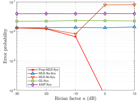
(a) $\kappa$ at $M=32$ and $L=48$.

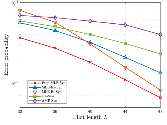
(b) $L$ at $M=32$.

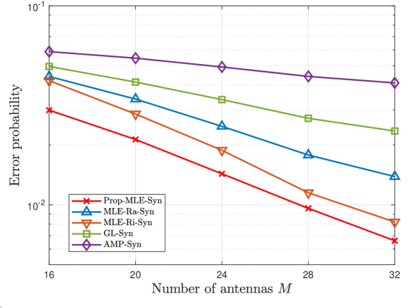
(c) $M$ at $L=48$.

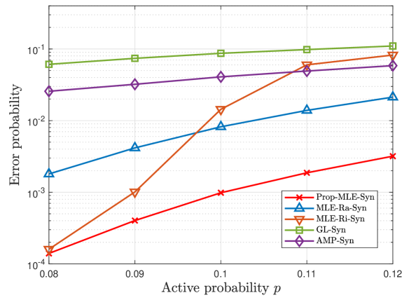
(d) $p$ at $N=2000$, $M=256$, and $\sigma=20$.

Figure 1: Error probability versus $\kappa$, $L$, $M$, and $p$ in the synchronous case.

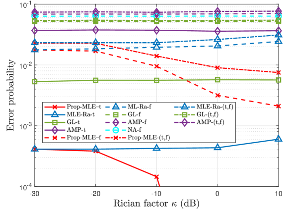
(a) $\kappa$.

(b) $L$.

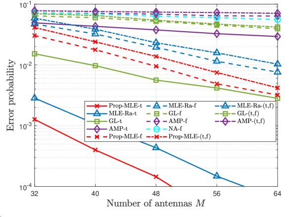
(c) $M$.

(d) $p$ at $N=2000$, $M=256$, and $\sigma=10$.

Figure 2: Error probability versus $\kappa$, $L$, $M$, and $p$ in the asynchronous cases.

Fig. 1 and Fig. 2 plot the error probability versus the Rician factor $\kappa$, pilot length $L$, and number of antennas $M$ in the synchronous case and three asynchronous cases, respectively. We can make the following observations from Fig. 1 (a) and Fig. 2 (a). Firstly, the error probabilities of Prop-MLE-$i$, $i\in$ {Syn, t, f, (t,f)} significantly decrease with $\kappa$. This is because the influences of the device activities and offsets on the p.d.f.s of received signals are larger when $\kappa$ is larger. Secondly, the error probabilities of MLE-Ra-$i$, $i\in$ {Syn, t, f, (t,f)} slightly increase with $\kappa$, as the errors caused by approximating Rician fading with Rayleigh fading increase with $\kappa$. Thirdly, the error probabilities of GL-$i$, AMP-$i$, $i\in$ {Syn, t, f, (t,f)}, and NA-f hardly change with $\kappa$, as group LASSO [11, 22] and the norm approximation-based method [24] do not rely on the channel model. Fourthly, when $\kappa\geq 1$, the error probabilities of MLE-Ri-Syn reach the active probability $p$, meaning that MLE-Ri-Syn does not work reasonably in this regime. From Fig. 1 (b), Fig. 2 (b), Fig. 1 (c), and Fig. 2 (c), we can see that the error probability of each method decreases with $L$, as the number of measurement vectors increases with $L$; and the error probability of each method decreases with $M$, as the number of observations increases with $M$. From Fig. 1 (d) and Fig. 2 (d), we can see that the error probability of each method decreases with $p$, as the interference between active devices increases with $p$.

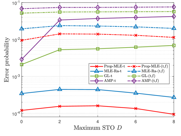
(a) $D$.

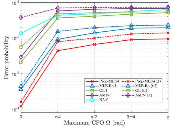
(b) $\Omega$.

Figure 3: Error probability versus $D$ and $\Omega$.

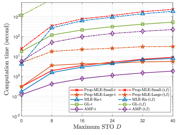
(a) $D$.

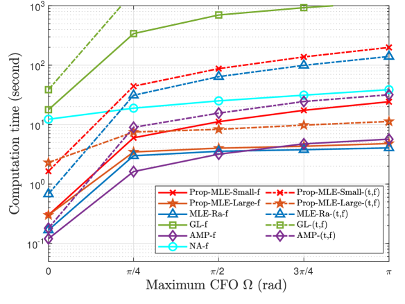
(b) $\Omega$.

Figure 4: Computation time versus $D$ and $\Omega$.

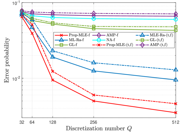
(a) Error probability versus $Q$.

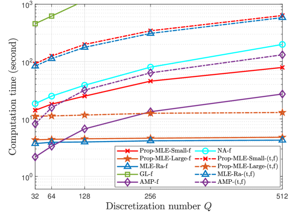
(b) Computation time versus $Q$.

Figure 5: Error probability and computation time versus $Q$.

Fig. 3 plots the error probability versus the maximum STO $D$ and the maximum CFO $\Omega$. The length of measurement vectors $\mathbf{Y}_{i,:,m}$ is $L_{i}=L+\mathbb{I}(i\neq\text{f})D$, for all $i\in$ {t, f, (t,f)} and $m\in\mathcal{M}$, and the number of possible STOs in $\hat{\mathcal{X}}_{\text{t}}$ and the number of possible CFOs in $\hat{\mathcal{X}}_{\text{f}}$ are $D+1$ and $2\lfloor\frac{Q\Omega}{2\pi}\rfloor+\mathbb{I}(\Omega\neq\pi)$, respectively. When $D$ increases, $L_{i}$ and $|\hat{\mathcal{X}}_{\text{t}}|$ increase; when $\Omega$ increases, $L_{i}$ does not change, and $|\hat{\mathcal{X}}_{\text{f}}|$ increases. In general, detection accuracy increases with the number of measurements but decreases with the number of candidates for an unknown parameter to be estimated. From Fig. 3 (a), we can observe that for $i\in$ {t, (t,f)}, the error probabilities of Prop-MLE-$i$ and MLE-Ra-$i$ (GL-$i$ and AMP-$i$) increase with $D$ when $D\in[0,2]$ ($D\in$ [0,8]), as the impact of the increment in the number of candidates for STOs on detection performance dominants that of the increment in the number of measurements in this regime; the error probabilities of Prop-MLE-$i$ and MLE-Ra-$i$ decrease with $D$ when $D\in[2,8]$, as the impact of the increment in the number of measurements on detection performance dominants that of the increment in the number of candidates for STOs in this regime. Besides, from Fig. 3 (b), we can observe that the error probabilities of Prop-MLE-$i$, MLE-Ra-$i$, GL-$i$, AMP-$i$, $i\in$ {f, (t,f)}, and NA-f increase with $\Omega$, due to the increment in the number of candidates for CFOs.

We can make the following observations from Fig. 1, Fig. 2, and Fig. 3. Firstly, in each case, the proposed method (on average) significantly outperforms all the baseline methods, revealing the proposed method’s superiority. Specifically, Prop-MLE-$i$ reduces the error probability by up to $50.4\%$, $65.8\%$, $51.3\%$, and $39.6\%$, compared to MLE-Ra-$i$ (the MLE-based state-of-the-art) for $i=$ Syn, t, f, and (t,f), respectively, at $\kappa=0.1$. The gain of Prop-MLE-$i$ over MLE-Ra-$i$ is because Prop-MLE-$i$ uses the exact channel statistics; and the gain of Prop-MLE-Syn over MLE-Ri-Syn comes from the fact that Prop-MLE-Syn deals with the original MLE problem, while MLE-Ri-Syn solves an approximate version of the MLE problem. Secondly, for $i\in$ {Syn, t, f, (t,f)}, the gain of Prop-MLE-$i$ over MLE-Ra-$i$ increases with $\kappa$, as the error of approximating Rician fading with Rayleigh fading increases with $\kappa$. Thirdly, for $\mu\in$ {Prop-MLE, AMP, MLE-Ra, LASSO}, $\mu$-(t,f) underperforms $\mu$-t and $\mu$-f, as the device activity detection problem in asynchronous case-(t,f) is more challenging than those in asynchronous case-t and asynchronous case-f (due to more unknowns to estimate).

Fig. 4 plots the computation time versus the maximum STO $D$ and the maximum CFO $\Omega$. We make the following observations from Fig. 4. Firstly, the computation time of Prop-MLE-Large-$i$ is comparable to that of to AMP-$i$ for all $i\in$ {Syn, t, f, (t,f)} and is even (on average) shorter than that of AMP-$i$ for $i\in$ {f, (t,f)} and large $D$ and $\Omega$. This result is appealing as AMP is known to be a highly efficient algorithm. Secondly, Prop-MLE-Large-$i$ has a shorter computation time than Prop-MLE-Small-$i$ for $i=$ t, f, and (t,f) when $D>22$, $\Omega>0.33\pi$, and $D>0$ or $\Omega>0.05\pi$, respectively, which is roughly in accordance with Lemma 4. Thirdly, compared to MLE-Ra-$i$, Prop-MLE-Large-$i$ can reduce the computation time by up to $29.8\%$ and $92.0\%$ for $i=$ t and (t,f), respectively. The gains come from the fact that the computational complexities of MLE-Ra-$i$ significantly increase with $D$ or/and $\Omega$, whereas the computational complexity of Prop-MLE-Large-$i$ does not change with $D$ or/and $\Omega$, as shown in TableIV. Fourthly, when $D=0$, the computation time of Prop-MLE-Small-t (reduces to Prop-MLE-Syn) is $78.6\%$ longer than that of MLE-Ra-t (reduces to MLE-Ra-Syn), as MLE-Ra-t considers Rayleigh fading as a substitute for simplicity.

Fig. 5 shows the error probability and computation time versus $Q$. From Fig. 5, we can see that Prop-MLE-Large-(t,f) (Prop-MLE-Large-f) achieves on average the best detection accuracy with on average the lowest (second lowest) computation time when $Q$ is large, demonstrating the high efficiency of Prop-MLE-Large-$i$, $i\in$ {f, (t,f)}. Specifically, from Fig. 5 (a), we can see that the error probability of each algorithm decreases with $Q$, due to the decrement in the approximation error with $Q$; from Fig. 5 (b), we can see that the computation time of each algorithm increases with $Q$, due to the increment in the number of CFO’s candidates.

In summary, combining the results on detection performance and computational time, we can conclude that the proposed solutions achieve the smallest detection error probabilities with (on average) the shortest computation times in some cases (i.e., asynchronous case-f and asynchronous case-(t,f) at large $D$ and $\Omega$) and relatively short computation times in other cases (i.e., the synchronous case and three asynchronous cases at small $D$ and $\Omega$).

VI Conclusion

This paper systematically investigated MLE-based device activity detection under Rician fading for massive grant-free access with perfect and imperfect synchronization. The proposed algorithms successfully generalized the existing MLE-based methods for Rayleigh fading and perfect synchronization. Numerical results demonstrated the superiority of the proposed algorithms in detection accuracy and computation time and the importance of explicit consideration of LoS components and synchronization errors in massive grant-free access. To our knowledge, this is the first work that systematically utilizes FFT and IFFT techniques to accelerate device activity detection algorithms for massive grant-free access. Besides, this is the first work comprehensively investigating MLE-based device activity detection under Rician fading for massive grant-free access.

There are still some key aspects that we leave for future investigations. One direction is to study MAPE-based device activity detection methods under flat Rician fading for massive grant-free with imperfect synchronization by utilizing prior information on device activities. Another interesting direction is to investigate MLE and MAPE-based device activity detection under frequency-selective Rayleigh and Rician fading for OFDM-based massive grant-free with imperfect synchronization.

Appendix A: Proof for Theorem 1

First, consider the coordinate optimization with respect to $a_{n}$ in (25). By (23), we have:

$$\begin{array}[]{ll}\quad f(\mathbf{a}_{-n},a_{n}+d_{n})\overset{(a)}{=}\log\left|\mathbf{\Sigma}+\frac{d_{n}g_{n}}{1+\kappa_{n}}{\mathbf{p}}_{n}{\mathbf{p}}_{n}^{H}\right|\end{array}$$ (56)

$$\begin{array}[]{ll}\quad+\frac{1}{M}\mathrm{tr}\left(\Big{(}\mathbf{\Sigma}+\frac{d_{n}g_{n}}{1+\kappa_{n}}{\mathbf{p}}_{n}{\mathbf{p}}_{n}^{H}\Big{)}^{-1}\Big{(}\widetilde{\mathbf{Y}}-d_{n}\sqrt{\frac{g_{n}\kappa_{n}}{1+\kappa_{n}}}{\mathbf{p}}_{n}\overline{\mathbf{h}}_{n}^{T}\Big{)}\Big{(}\widetilde{\mathbf{Y}}-d_{n}\sqrt{\frac{g_{n}\kappa_{n}}{1+\kappa_{n}}}{\mathbf{p}}_{n}\overline{\mathbf{h}}_{n}^{T}\Big{)}^{H}\right)\end{array}$$ (58)

$$\begin{array}[]{ll}&\overset{(b)}{=}\log\Big{(}|\mathbf{\Sigma}|(1+\frac{d_{n}g_{n}}{1+\kappa_{n}}{\bf p}_{n}^{H}{\bf\Sigma}^{-1}{\bf p}_{n})\Big{)}\\ &+\frac{1}{M}\mathrm{tr}\Big{(}\Big{(}\mathbf{\Sigma}^{-1}-\frac{\frac{d_{n}g_{n}}{1+\kappa_{n}}\mathbf{\Sigma}^{-1}{\mathbf{p}}_{n}{\mathbf{p}}_{n}^{H}\mathbf{\Sigma}^{-1}}{1+\frac{d_{n}g_{n}}{1+\kappa_{n}}{\bf p}_{n}^{H}{\bf\Sigma}^{-1}{\bf p}_{n}}\Big{)}\Big{(}\widetilde{\mathbf{Y}}-d_{n}\sqrt{\frac{g_{n}\kappa_{n}}{1+\kappa_{n}}}{\mathbf{p}}_{n}\overline{\mathbf{h}}_{n}^{T}\Big{)}\Big{(}\widetilde{\mathbf{Y}}-d_{n}\sqrt{\frac{g_{n}\kappa_{n}}{1+\kappa_{n}}}{\mathbf{p}}_{n}\overline{\mathbf{h}}_{n}^{T}\Big{)}^{H}\Big{)}\\ &{\color[rgb]{0,0,0}=f(\mathbf{a})+\log\Big{(}1+\frac{dg_{n}}{1+\kappa_{n}}{\bf p}_{n}^{H}{\bf\Sigma}^{-1}{\bf p}_{n}\Big{)}+\frac{d_{n}^{2}g_{n}\kappa_{n}}{1+\kappa_{n}}{\bf p}_{n}^{H}{\bf\Sigma}^{-1}{\bf p}_{n}-\frac{d_{n}}{M}\sqrt{\frac{g_{n}\kappa_{n}}{1+\kappa_{n}}}\left(\mathrm{tr}\left({\bf\Sigma}^{-1}{\mathbf{p}}_{n}\overline{\mathbf{h}}_{n}^{T}\widetilde{\mathbf{Y}}^{H}\right)+\mathrm{tr}\left({\bf\Sigma}^{-1}\widetilde{\mathbf{Y}}\overline{\mathbf{h}}_{n}^{*}{\mathbf{p}}^{H}_{n}\right)\right)}\\ &\quad{\color[rgb]{0,0,0}+\frac{\frac{d_{n}^{2}}{M}(\frac{g_{n}\kappa_{n}}{1+\kappa_{n}})^{\frac{3}{2}}\left(\mathrm{tr}\left({\bf\Sigma}^{-1}{\mathbf{p}}_{n}{\mathbf{p}}_{n}^{H}{\bf\Sigma}^{-1}{\mathbf{p}}_{n}\overline{\mathbf{h}}_{n}^{T}\widetilde{\mathbf{Y}}^{H}\right)+\mathrm{tr}\left({\bf\Sigma}^{-1}{\mathbf{p}}_{n}{\mathbf{p}}_{n}^{H}{\bf\Sigma}^{-1}\widetilde{\mathbf{Y}}\overline{\mathbf{h}}_{n}^{*}{\mathbf{p}}^{H}_{n}\right)\right)}{1+\frac{d_{n}g_{n}}{1+\kappa_{n}}{\bf p}_{n}^{H}{\bf\Sigma}^{-1}{\bf p}_{n}}}\\ &\quad{\color[rgb]{0,0,0}-\!\frac{\frac{d_{n}g_{n}}{M(1+\kappa_{n})}{\bf p}_{n}^{H}{\bf\Sigma}^{-1}\widetilde{\mathbf{Y}}\widetilde{\mathbf{Y}}^{H}{\bf\Sigma}^{-1}{\bf p}_{n}+\frac{1}{M(1+\kappa_{n})^{2}}d_{n}^{3}g_{n}^{2}\kappa_{n}\mathrm{tr}\left({\bf\Sigma}^{-1}{\mathbf{p}}_{n}{\mathbf{p}}_{n}^{H}{\bf\Sigma}^{-1}{\mathbf{p}}_{n}\overline{\mathbf{h}}_{n}^{T}\overline{\mathbf{h}}_{n}^{*}{\mathbf{p}}_{n}^{H}\right)}{1+\frac{d_{n}g_{n}}{1+\kappa_{n}}{\bf p}_{n}^{H}{\bf\Sigma}^{-1}{\bf p}_{n}}}\\ &\overset{(c)}{=}f(\mathbf{a})+\log\Big{(}1+\frac{g_{n}}{1+\kappa_{n}}{\bf p}_{n}^{H}{\bf\Sigma}^{-1}{\bf p}_{n}d_{n}\Big{)}+\frac{d_{n}}{1+\frac{g_{n}}{1+\kappa_{n}}{\bf p}_{n}^{H}{\bf\Sigma}^{-1}{\bf p}_{n}d_{n}}\times\Big{(}\frac{g_{n}\kappa_{n}}{1+\kappa_{n}}{\bf p}_{n}^{H}{\bf\Sigma}^{-1}{\bf p}_{n}d_{n}\\ &-\frac{g_{n}}{M(1+\kappa_{n})}{\bf p}_{n}^{H}{\bf\Sigma}^{-1}\widetilde{\mathbf{Y}}\widetilde{\mathbf{Y}}^{H}{\bf\Sigma}^{-1}{\bf p}_{n}-\frac{2}{M}\sqrt{\frac{g_{n}\kappa_{n}}{1+\kappa_{n}}}\mathrm{Re}\left(\overline{\bf h}_{n}^{T}\widetilde{\mathbf{Y}}^{H}{\bf\Sigma}^{-1}{\bf p}_{n}\right)\Big{)}\end{array}$$ (61)

$$\!\quad\begin{array}[]{ll}\overset{(d)}{=}f(\mathbf{a})+\log(1+\alpha_{n}d_{n})+\frac{\kappa_{n}\alpha_{n}d_{n}^{2}-(\beta_{n}+\eta_{n})d_{n}}{1+\alpha_{n}d_{n}},\end{array}$$ (63)

where (a) is due to ${\bf\Sigma}=\mathbf{P}\mathbf{A}\mathbf{\Gamma}\mathbf{P}^{H}+\sigma^{2}{\bf I}_{L}$ and $\widetilde{\mathbf{Y}}=\mathbf{Y}-{\mathbf{P}}{\bf A}{\bf\Gamma}^{\frac{1}{2}}\overline{\bf H}^{T}$, (b) is due to the fact that for any positive definite matrix $\mathbf{\Sigma}$, $|\mathbf{\Sigma}+\frac{d_{n}g_{n}}{1+\kappa_{n}}{\mathbf{p}}_{n}{\mathbf{p}}_{n}^{H}|=|\mathbf{\Sigma}|(1+\frac{d_{n}g_{n}}{1+\kappa_{n}}{\bf p}_{n}^{H}{\bf\Sigma}^{-1}{\bf p}_{n})$ and $\left(\mathbf{\Sigma}+\frac{d_{n}g_{n}}{1+\kappa_{n}}{\mathbf{p}}_{n}{\mathbf{p}}_{n}^{H}\right)^{-1}=\mathbf{\Sigma}^{-1}-\frac{\frac{d_{n}g_{n}}{1+\kappa_{n}}\mathbf{\Sigma}^{-1}{\mathbf{p}}_{n}{\mathbf{p}}_{n}^{H}\mathbf{\Sigma}^{-1}}{1+\frac{d_{n}g_{n}}{1+\kappa_{n}}{\bf p}_{n}^{H}{\bf\Sigma}^{-1}{\bf p}_{n}}$ hold [7], (c) is due to

$$\frac{1}{M}\mathrm{tr}\Big{(}{\bf\Sigma}^{-1}{\mathbf{p}}_{n}\overline{\mathbf{h}}_{n}^{T}\overline{\mathbf{h}}_{n}^{*}{\mathbf{p}}_{n}^{H}\Big{)}={\bf p}_{n}^{H}{\bf\Sigma}^{-1}{\bf p}_{n},$$

$$\mathrm{tr}\Big{(}{\bf\Sigma}^{-1}{\mathbf{p}}_{n}{\mathbf{p}}_{n}^{H}{\bf\Sigma}^{-1}{\mathbf{p}}_{n}\overline{\mathbf{h}}_{n}^{T}\widetilde{\mathbf{Y}}^{H}\Big{)}+\mathrm{tr}\Big{(}{\bf\Sigma}^{-1}{\mathbf{p}}_{n}{\mathbf{p}}_{n}^{H}{\bf\Sigma}^{-1}\widetilde{\mathbf{Y}}\overline{\mathbf{h}}_{n}^{*}{\mathbf{p}}^{H}_{n}\Big{)}=2\left({\bf p}_{n}^{H}{\bf\Sigma}^{-1}{\bf p}_{n}\right)\left(\mathrm{Re}\Big{(}\overline{\bf h}_{n}^{T}\widetilde{\mathbf{Y}}^{H}{\bf\Sigma}^{-1}{\bf p}_{n}\Big{)}\right),$$

$$\frac{1}{M}\mathrm{tr}\Big{(}{\bf\Sigma}^{-1}{\mathbf{p}}_{n}{\mathbf{p}}_{n}^{H}{\bf\Sigma}^{-1}{\mathbf{p}}_{n}\overline{\mathbf{h}}_{n}^{T}\overline{\mathbf{h}}_{n}^{*}{\mathbf{p}}_{n}^{H}\Big{)}=\left({\bf p}_{n}^{H}{\bf\Sigma}^{-1}{\bf p}_{n}\right)^{2},$$

and (d) is due to (26),  (27), and (28). By (63), we have:

$$\frac{\partial f(\mathbf{a}_{-n},a_{n}+d_{n})}{\partial d_{n}}=\frac{\kappa_{n}\alpha_{n}^{2}d_{n}^{2}+\left(\alpha_{n}^{2}+2\kappa_{n}\alpha_{n}\right)d_{n}+\alpha_{n}-\beta_{n}-\eta_{n}}{(1+\alpha_{n}d_{n})^{2}}.$$

Note that the domain of $f(\mathbf{a}_{-n},a_{n}+d_{n})$ with respect to $d_{n}$ is $(-\frac{1}{\alpha_{n}},+\infty)$. In the following, we obtain the optimal solution of problem in (25) by analyzing the monotonicity of $f(\mathbf{a}_{-n},a_{n}+d_{n})$ in the domain $(-\frac{1}{\alpha_{n}},+\infty)\cap[-a_{n},1-a_{n}]$. Since solving $\frac{\partial f(\mathbf{a}_{-n},a_{n}+d_{n})}{\partial d_{n}}=0$ is equivalent to solving $q(d_{n})\triangleq\kappa_{n}\alpha_{n}^{2}d_{n}^{2}+\left(\alpha_{n}^{2}+2\kappa_{n}\alpha_{n}\right)d_{n}+\alpha_{n}-\beta_{n}-\eta_{n}=0$, we analyze the monotonicity of $f(\mathbf{a}_{-n},a_{n}+d_{n})$ by analyzing the roots of $q(d_{n})=0$ in two cases. If $\alpha_{n}^{2}+4\kappa_{n}(\kappa_{n}+\beta_{n}+\eta_{n})\leq 0$, then $q(d_{n})=0$ has at most one root (as $\kappa_{n}\alpha_{n}^{2}>0$). Hence, $q(d_{n})\geq 0$ for all $d_{n}\in(-\frac{1}{\alpha_{n}},+\infty)$, implying that $f(\mathbf{a}_{-n},a_{n}+d_{n})$ increases with $d_{n}$ when $d_{n}\in(-\frac{1}{\alpha_{n}},+\infty)$. Combining with the constraint $d_{n}\in[-a_{n},1-a_{n}]$, we have the optimal solution given in (31). If $\alpha_{n}^{2}+4\kappa_{n}(\kappa_{n}+\beta_{n}+\eta_{n})>0$, then $q(d_{n})=0$ has two roots: one is $\hat{d}_{n}$ given by (32), and the other one is $\frac{-\alpha_{n}-2\kappa_{n}-\sqrt{\alpha_{n}^{2}+4\kappa_{n}(\kappa_{n}+\beta_{n}+\eta_{n})}}{2\kappa_{n}\alpha_{n}}<-\frac{1}{\alpha_{n}}$. If $\hat{d}_{n}\leq-\frac{1}{\alpha_{n}}$, then $q(d_{n})\geq 0$ for all $d_{n}\in(-\frac{1}{\alpha_{n}},+\infty)$, implying that $f(\mathbf{a}_{-n},a_{n}+d_{n})$ increases with $d_{n}$ when $d_{n}\in(-\frac{1}{\alpha_{n}},+\infty)$; If $\hat{d}_{n}>-\frac{1}{\alpha_{n}}$, then $q(d_{n})<0$ for all $d_{n}\in(-\frac{1}{\alpha_{n}},\hat{d}_{n})$ and $q(d_{n})\geq 0$ for all $d_{n}\in[\hat{d}_{n},+\infty)$, implying that $f(\mathbf{a}_{-n},a_{n}+d_{n})$ decreases with $d_{n}$ when $d_{n}\in(-\frac{1}{\alpha_{n}},\hat{d}_{n})$, increases with $d_{n}$ when $d_{n}\in(\hat{d}_{n},+\infty)$, and achieves its minimum at $d_{n}=\hat{d}_{n}$. Combining with the constraint $d_{n}\in[-a_{n},1-a_{n}]$, we have the optimal solution given in (31).

Appendix B: Proof for Theorem 2

Note that $f(\mathbf{a})$ is continuously differentiable with respect to $\mathbf{a}$, and the constraints for $\mathbf{a}$ are convex. According to the proof of Theorem 1, each optimal coordinate is uniquely obtained, and $f(\mathbf{a}_{-n},a_{n})$ is monotonically nonincreasing in the interval from $a_{n}$ to $a_{n}+d_{n}^{*}$. Thus, the assumptions of [34, Proposition 3.7.1] are satisfied. Therefore, we can show Theorem 2 by [34, Proposition 3.7.1].

Appendix C: Proof for Theorem 3

Note that $\min_{a\in[0,1],x\in\hat{\mathcal{X}}_{i}}f_{i}(\mathbf{a}_{-n},a,\mathbf{x}_{i,-n},x)=\min_{x\in\hat{\mathcal{X}}_{i}}\min_{a\in[0,1]}f_{i}(\mathbf{a}_{-n},a,\mathbf{x}_{i,-n},x)$. First, we solve $\min_{a\in[0,1]}f_{i}(\mathbf{a}_{-n},a,\mathbf{x}_{i,-n},x)$ for any given $x\in\hat{\mathcal{X}}_{i}$. By (24), we have:

$$f_{i}(\mathbf{a}_{-n},a,\mathbf{x}_{i,-n},x)\overset{(a)}{=}\log\left|\mathbf{\Sigma}_{i,n}+\frac{ag_{n}}{1+\kappa_{n}}{\bf p}_{i,n}(x){\bf p}^{H}_{i,n}(x)\right|+\frac{1}{M}\mathrm{tr}\Big{(}\Big{(}\mathbf{\Sigma}_{i,n}+\frac{ag_{n}}{1+\kappa_{n}}{\bf p}_{i,n}(x){\bf p}^{H}_{i,n}(x)\Big{)}^{-1}$$

$$\times\Big{(}\widetilde{\mathbf{Y}}_{i,n}-a\sqrt{\frac{g_{n}\kappa_{n}}{1+\kappa_{n}}}\mathbf{p}_{i,n}(x)\overline{\mathbf{h}}_{n}^{T}\Big{)}\Big{(}\widetilde{\mathbf{Y}}_{i,n}-a\sqrt{\frac{g_{n}\kappa_{n}}{1+\kappa_{n}}}\mathbf{p}_{i,n}(x)\overline{\mathbf{h}}_{n}^{T}\Big{)}^{H}\Big{)}$$

$$\overset{(b)}{=}f_{i}(\mathbf{a}_{-n},0,\mathbf{x}_{i,-n},0)+\log(1+\alpha_{i,n}(x)a)+\frac{\kappa_{n}\alpha_{i,n}(x)a^{2}-(\beta_{i,n}(x)+\eta_{i,n}(x))a}{1+\alpha_{i,n}(x)a},$$ (64)

where (a) is due to ${\bf\Sigma}_{i}=\mathbf{\Sigma}_{i,n}+\frac{ag_{n}}{1+\kappa_{n}}{\bf p}_{i,n}(x){\bf p}^{H}_{i,n}(x)$ and $\widetilde{\mathbf{Y}}_{i}=\widetilde{\mathbf{Y}}_{i,n}-a\sqrt{\frac{g_{n}\kappa_{n}}{1+\kappa_{n}}}\mathbf{p}_{i,n}(x)\overline{\mathbf{h}}_{n}^{T}$, and (b) follows from (63) (by regarding ${\mathbf{p}}_{i,n}(x)$, $\mathbf{\Sigma}_{i,n}$, and $\overline{\mathbf{Y}}_{i,n}$ in (64) as ${\mathbf{p}}_{n}$, $\mathbf{\Sigma}$, and $\overline{\mathbf{Y}}$ in (63), respectively). Thus, following the proof for Theorem 1, we can readily show that at any given $x\in\hat{\mathcal{X}}_{i}$, the optimal solution and optimal value of $\min_{a\in[0,1]}f_{i}(\mathbf{a}_{-n},a,\mathbf{x}_{i,-n},x)$ are $d_{i,n}(x)$ in (39) and $f_{i}(\mathbf{a}_{-n},d_{i,n}(x),\mathbf{x}_{i,-n},x)=f_{i}(\mathbf{a}_{-n},0,\mathbf{x}_{i,-n},0)+h_{i,n}(x)$, respectively, where $h_{i,n}(x)$ is given in (40). It remains to solve $\min_{x\in\hat{\mathcal{X}}_{i}}$ $f_{i}(\mathbf{a}_{-n},d_{i,n}(x),\mathbf{x}_{i,-n},x)$, which is equivalent to $\min_{x\in\hat{\mathcal{X}}_{i}}h_{i,n}(x)$. Therefore, we have the optimal solution given in (36).

Appendix D: Proof for Lemma 1

For all $\omega\in\mathbb{R}$, $\mathbf{p}\in\mathbb{C}^{K}$, and Hermitian matrix $\mathbf{B}\in\mathbb{C}^{K\times K}$, let $J(\omega,\mathbf{p},\mathbf{B})\triangleq\mathbf{p}^{H}\mathrm{diag}((e^{j(k-1)\omega})_{k\in\mathcal{K}})^{H}$ $\mathbf{B}\mathrm{diag}((e^{j(k-1)\omega})_{k\in\mathcal{K}})\mathbf{p}$. Recall that $\boldsymbol{\Psi}(\mathbf{B})=(\boldsymbol{\psi}_{k}(\mathbf{B}))_{k\in\mathcal{K}}\in\mathbb{C}^{K\times K}$, where $\boldsymbol{\psi}_{k}(\mathbf{B})\in\mathbb{C}^{K}$ is given in (43). To prove Lemma 1, we need the following matrix identities:

$$\mathrm{diag}(\mathbf{u})\mathbf{v}=\mathrm{diag}(\mathbf{v})\mathbf{u}=\mathbf{u}\odot\mathbf{v}=\mathbf{v}\odot\mathbf{u},\ \mathbf{u},\mathbf{v}\in\mathbb{C}^{K},$$ (65)

$$\mathrm{diag}(\mathbf{u})\mathbf{B}\mathrm{diag}(\mathbf{v})=\mathbf{B}\odot(\mathbf{u}\mathbf{v}^{T}),\ \ \mathbf{u},\mathbf{v}\in\mathbb{C}^{K},$$ (66)

$$(\mathbf{w}_{q}^{T}(\mathbf{u}_{t,k}^{T}\mathbf{v}_{k})_{k\in\mathcal{K}})_{t\in\mathcal{K},q\in\mathcal{K}}=(((\mathbf{u}_{t,k})_{t\in\mathcal{K}})^{T}\mathbf{v}_{k})_{k\in\mathcal{K}}(\mathbf{w}_{q})_{q\in\mathcal{K}},\ \mathbf{w}_{q},\mathbf{u}_{t,k},\mathbf{v}_{k}\in\mathbb{C}^{K},t,q,k\in\mathcal{K},$$ (67)

$$(\mathbf{B}(\mathbf{u}_{k}\odot\mathbf{v}_{k}))_{k\in\mathcal{K}}=\mathbf{B}\left((\mathbf{u}_{k})_{k\in\mathcal{K}}\odot(\mathbf{v}_{k})_{k\in\mathcal{K}}\right),\ \ \mathbf{u}_{k},\mathbf{v}_{k}\in\mathbb{C}^{K},k\in\mathcal{K}.$$ (68)

The proofs for (65)-(68) are obvious and hence omitted. First, we show an equality based on which we will show (44) and (45):

$$J(\omega,\mathbf{p},\mathbf{B})\overset{(a)}{=}\left((e^{j(k-1)\omega})_{k\in\mathcal{K}}\right)^{H}\mathrm{diag}(\mathbf{p}^{*})\mathbf{B}\mathrm{diag}(\mathbf{p})\left(e^{j(k-1)\omega}\right)_{k\in\mathcal{K}}$$

$$\overset{(b)}{=}\mathrm{tr}\left((\mathbf{B}\odot(\mathbf{p}^{*}\mathbf{p}^{T}))\left((e^{j(\ell-1)\omega})_{\ell\in\mathcal{K}}\right)\left((e^{j(k-1)\omega})_{k\in\mathcal{K}}\right)^{H}\right)=\sum\limits_{\ell=1}^{K}\sum\limits_{k=1}^{K}e^{j(k-\ell)\omega}(\mathbf{B}\odot(\mathbf{p}^{*}\mathbf{p}^{T}))_{\ell,k}$$

$$\overset{(c)}{=}2\mathrm{Re}\Big{(}e^{j0\omega}\sum\limits_{\ell=1}^{K-0}\Big{(}\frac{\sqrt{2}}{2}\mathbf{B}\odot\Big{(}\frac{\sqrt{2}}{2}\mathbf{p}^{*}\mathbf{p}^{T}\Big{)}\Big{)}_{k,k}+\sum\limits_{k=1}^{K-1}e^{jk\omega}\sum\limits_{\ell=1}^{K-k}(\mathbf{B}\odot(\mathbf{p}^{*}\mathbf{p}^{T}))_{\ell,\ell+k}\Big{)}$$

$$=2\mathrm{Re}\Big{(}\left((e^{j(\ell-1)\omega})_{\ell\in\mathcal{K}}\right)^{T}\Big{(}\boldsymbol{\psi}_{k}^{T}(\mathbf{p}^{*}\mathbf{p}^{T})\boldsymbol{\psi}_{k}(\mathbf{B})\Big{)}_{k\in\mathcal{K}}\Big{)},$$ (69)

where (a) is due to (65), (b) is due to (66), $x=\mathrm{tr}(x)$ for $x\in\mathbb{C}$, and the cyclic property of trace, and (c) is due to that $\mathbf{B}\odot(\mathbf{p}^{*}\mathbf{p}^{T})$ is a Hermitian matrix (as $\mathbf{B}$ and $\mathbf{p}^{*}\mathbf{p}^{T}$ are Hermitian matrices). Then, by (69), we show (44) as follows:

$$\frac{1+\kappa_{n}}{2g_{n}}\boldsymbol{\alpha}_{\text{t},n}\overset{(a)}{=}\frac{1}{2}\left(J(0,\mathbf{p}_{\text{t},n}(t),\mathbf{\Sigma}_{\text{t},n}^{-1})\right)_{t\in\mathcal{D}}$$

$$\overset{(b)}{=}\left(\mathrm{Re}\left(\mathbf{1}_{L_{\text{t}}}^{T}\left(\boldsymbol{\psi}_{\ell}^{T}\Big{(}\mathbf{p}_{\text{t},n}^{*}(t)\mathbf{p}_{\text{t},n}^{T}(t)\Big{)}\boldsymbol{\psi}_{\ell}({\mathbf{\Sigma}}_{\text{t},n}^{-1})\right)_{\ell\in\mathcal{L}_{\text{t}}}\right)\right)_{t\in\mathcal{D}}$$

$$\overset{(c)}{=}\mathrm{Re}\left(\!\left(\!\left(\!\Big{(}\boldsymbol{\psi}_{\ell}\Big{(}\mathbf{p}_{\text{t},n}^{*}(t)\mathbf{p}_{\text{t},n}^{T}(t)\Big{)}\Big{)}_{t\in\mathcal{D}}\right)^{T}\!\!\boldsymbol{\psi}_{\ell}({\mathbf{\Sigma}}_{\text{t},n}^{-1})\right)_{\ell\in\mathcal{L}_{\text{t}}}\!\!\!\!\!\mathbf{1}_{L_{\text{t}}}\right)$$ (70)

$$\overset{(d)}{=}\mathrm{Re}\Big{(}\Big{(}\mathbf{F}_{L_{\text{t}},\widetilde{\mathcal{D}},:}\mathrm{diag}\Big{(}\mathbf{F}_{L_{\text{t}}}\boldsymbol{\psi}_{\ell}\Big{(}\mathbf{p}_{\text{t},n}^{*}(0)\mathbf{p}_{\text{t},n}^{T}(0)\Big{)}\Big{)}\frac{1}{L_{\text{t}}}\mathbf{F}_{L_{\text{t}}}^{H}\boldsymbol{\psi}_{\ell}({\mathbf{\Sigma}}_{\text{t},n}^{-1})\Big{)}_{\ell\in\mathcal{L}_{\text{t}}}\mathbf{1}_{L_{\text{t}}}\Big{)}$$ (71)

$$\overset{(e)}{=}\bigg{(}\mathrm{Re}\Big{(}\mathbf{F}_{L_{\text{t}}}\Big{(}\Big{(}\frac{1}{L_{\text{t}}}\mathbf{F}_{L_{\text{t}}}^{H}\boldsymbol{\Psi}({\mathbf{\Sigma}}_{\text{t},n}^{-1})\Big{)}\odot\Big{(}\mathbf{F}_{L_{\text{t}}}\boldsymbol{\Psi}\big{(}\mathbf{p}_{\text{t},n}^{*}(0)\mathbf{p}_{\text{t},n}^{T}(0)\big{)}\Big{)}\Big{)}\mathbf{1}_{L_{\text{t}}}\Big{)}\bigg{)}_{\widetilde{\mathcal{D}}},$$ (72)

where (a) is due to (31), (b) is due to (69), (c) is due to (67), (d) is due to

$$\left(\left(\boldsymbol{\psi}_{\ell}\left(\mathbf{p}_{\text{t},n}^{*}(t)\mathbf{p}_{\text{t},n}^{T}(t)\right)\right)_{t\in\mathcal{D}}\right)_{k,m}=\left(\boldsymbol{\psi}_{\ell}\left(\mathbf{p}_{\text{t},n}^{*}(0)\mathbf{p}_{\text{t},n}^{T}(0)\right)\right)_{1+((L_{\text{t}}+k-m)\bmod L_{\text{t}})},\ k\in{\mathcal{L}}_{\text{t}},m\in\widetilde{\mathcal{D}},$$

and the eigen-decompositions of circulant matrices, and (e) is due to (65) and (68). Next, by noting that $\boldsymbol{\beta}_{\text{t},n}=\frac{g_{n}}{1+\kappa_{n}}(J(0,\mathbf{p}_{\text{t},n}(t),\mathbf{\Sigma}_{\text{t},n}^{-1}\widetilde{\mathbf{Y}}_{\text{t}}\widetilde{\mathbf{Y}}_{\text{t}}^{H}\mathbf{\Sigma}_{\text{t},n}^{-1}))_{t\in\hat{\mathcal{X}}_{\text{t}}}$, we can show (45) following the proof for (44). Finally, we show (46) as follows:

$$\frac{M}{2}\sqrt{\frac{1+\kappa_{n}}{g_{n}\kappa_{n}}}\boldsymbol{\eta}_{\text{t},n}\overset{(a)}{=}\mathrm{Re}\left(\Big{(}\Big{(}\mathbf{p}_{\text{t},n}(t)\Big{)}_{t\in\mathcal{D}}\Big{)}^{T}\Big{(}\overline{\bf h}_{n}^{T}\overline{\mathbf{Y}}_{\text{t},n}^{H}{\bf\Sigma}_{\text{t},n}^{-1}\Big{)}^{T}\right)$$

$$\overset{(b)}{=}\mathrm{Re}\Big{(}\mathbf{F}_{L_{\text{t}},\widetilde{\mathcal{D}},:}\mathrm{diag}\Big{(}\mathbf{F}_{L_{\text{t}}}\mathbf{p}_{\text{t},n}(0)\Big{)}\frac{1}{L_{\text{t}}}\mathbf{F}_{L_{\text{t}}}^{H}\Big{(}\overline{\bf h}_{n}^{T}\overline{\mathbf{Y}}_{\text{t},n}^{H}{\bf\Sigma}_{\text{t},n}^{-1}\Big{)}^{T}\Big{)}$$

$$\overset{(c)}{=}\left(\mathrm{Re}\Big{(}\mathbf{F}_{L_{\text{t}}}\left(\frac{1}{L_{\text{t}}}\mathbf{F}_{L_{\text{t}}}^{H}(\overline{\bf h}_{n}^{T}\widetilde{\mathbf{Y}}_{\text{t},n}^{H}{\bf\Sigma}_{\text{t},n}^{-1})^{T}\right)\odot\Big{(}\mathbf{F}_{L_{\text{t}}}\mathbf{p}_{\text{t},n}(0)\Big{)}\Big{)}\right)_{\widetilde{\mathcal{D}}},$$

where (a) is due to (33), (b) is due to $\left((\mathbf{p}_{\text{t},n}(t))_{t\in\mathcal{D}}\right)_{k,m}=\left(\mathbf{p}_{\text{t},n}(0)\right)_{1+(L_{\text{t}}+k-m)\bmod L_{\text{t}}}$, $k\in{\mathcal{L}}_{\text{t}},m\in\widetilde{\mathcal{D}}$ and the eigen-decompositions of circulant matrices, and (c) is due to (65).

Appendix E: Proof for Lemma 2

First, we show (47) as follows:

$$\frac{1+\kappa_{n}}{2g_{n}}\boldsymbol{\alpha}_{\text{f},n}\overset{(a)}{=}\frac{1}{2}\left(J(\omega,\mathbf{p}_{n},\mathbf{\Sigma}_{\text{f},n}^{-1})\right)_{\omega\in\hat{\mathcal{X}}_{\text{f}}}$$

$$\overset{(b)}{=}\left(\mathrm{Re}\left(\boldsymbol{\tau}_{\text{f}}^{T}\left(\omega^{(q)}\right)\Big{(}\boldsymbol{\psi}_{\ell}^{T}\left(\mathbf{p}_{n}^{*}\mathbf{p}_{n}^{T}\right)\boldsymbol{\psi}_{\ell}\left({\mathbf{\Sigma}}_{\text{f},n}^{-1}\right)\Big{)}_{\ell\in\mathcal{L}_{\text{f}}}\right)\right)_{{q\in\mathcal{Q}}}$$

$$\overset{(c)}{=}\mathrm{Re}\left(\left(\left(\boldsymbol{\tau}_{\text{f}}(\omega^{(q)})\right)_{q\in\mathcal{Q}}\right)^{T}\Big{(}\boldsymbol{\psi}_{\ell}^{T}\left(\mathbf{p}_{n}^{*}\mathbf{p}_{n}^{T}\right)\boldsymbol{\psi}_{\ell}\left({\mathbf{\Sigma}}_{\text{f},n}^{-1}\right)\Big{)}_{\ell\in\mathcal{L}_{\text{f}}}\right)$$

$$\overset{(d)}{=}\mathrm{Re}\left(\mathbf{T}_{\text{f},\mathcal{Q},:}\Big{(}\boldsymbol{\Psi}\left({\mathbf{\Sigma}}_{\text{f},n}^{-1}\right)\odot\boldsymbol{\Psi}\left(\mathbf{p}_{n}^{*}\mathbf{p}_{n}^{T}\right)\Big{)}^{T}\mathbf{1}_{L_{\text{f}}}\right)$$

$$=\left(\mathrm{Re}\left(\mathbf{T}_{\text{f}}\Big{(}\boldsymbol{\Psi}({\mathbf{\Sigma}}_{\text{f},n}^{-1})\odot\boldsymbol{\Psi}(\mathbf{p}_{n}^{*}\mathbf{p}_{n}^{T})\Big{)}^{T}\mathbf{1}_{L_{\text{f}}}\right)\right)_{\mathcal{Q}},$$

where (a) is due to (31), (b) is due to (69), (c) is due to (67), and (d) is due to $\left(\left(\boldsymbol{\tau}_{\text{f}}(\omega^{(q)})\right)_{q\in\mathcal{Q}}\right)^{T}=\mathbf{T}_{\text{f},\mathcal{Q},:}$ and the identity $(\mathbf{u}^{T}_{k}\mathbf{v}_{k})_{k\in\mathcal{K}}=\left((\mathbf{v}_{k})_{k\in\mathcal{K}}\odot(\mathbf{u}_{k})_{k\in\mathcal{K}}\right)^{T}\mathbf{1}_{K}$, for $\mathbf{u}_{k},\mathbf{v}_{k}\in\mathbb{C}^{K},k\in\mathcal{K}$. Next, by noting that $\boldsymbol{\beta}_{\text{f},n}=\frac{g_{n}}{1+\kappa_{n}}(J(\omega,\mathbf{p}_{n},$ $\mathbf{\Sigma}_{\text{f},n}^{-1}\widetilde{\mathbf{Y}}_{\text{f}}\widetilde{\mathbf{Y}}_{\text{f}}^{H}\mathbf{\Sigma}_{\text{f},n}^{-1}))_{\omega\in\hat{\mathcal{X}}_{\text{f}}}$, we can show (48) following the proof for (47). Finally, we show (49) as follows:

$$\frac{M}{2}\sqrt{\frac{1+\kappa_{n}}{g_{n}\kappa_{n}}}\boldsymbol{\eta}_{\text{f},n}\overset{(a)}{=}\left(\mathrm{Re}\Big{(}(\boldsymbol{\tau}_{\text{f}}(\omega))^{T}\Big{(}\overline{\bf h}_{n}^{T}\overline{\mathbf{Y}}_{\text{f},n}^{H}{\bf\Sigma}_{\text{f},n}^{-1}\mathrm{diag}(\mathbf{p}_{n})\Big{)}^{T}\Big{)}\right)_{\omega\in\mathcal{X}_{\text{f}}}$$

$$=\mathrm{Re}\left(\Big{(}\Big{(}\boldsymbol{\tau}_{\text{f}}(\omega^{(q)})\Big{)}_{q\in\mathcal{Q}}\Big{)}^{T}\Big{(}\overline{\bf h}_{n}^{T}\overline{\mathbf{Y}}_{\text{f},n}^{H}{\bf\Sigma}_{\text{f},n}^{-1}\mathrm{diag}(\mathbf{p}_{n})\Big{)}^{T}\right)$$

$$\overset{(b)}{=}\left(\mathrm{Re}\left(\mathbf{T}_{\text{f}}\left((\overline{\bf h}_{n}^{T}\widetilde{\mathbf{Y}}_{\text{f},n}^{H}{\bf\Sigma}_{\text{f},n}^{-1})^{T}\odot\mathbf{p}_{n}\right)\right)\right)_{\mathcal{Q}},$$

where (a) is due to (33), and (b) is due to $\left(\left(\boldsymbol{\tau}_{\text{f}}(\omega^{(q)})\right)_{q\in\mathcal{Q}}\right)^{T}=\mathbf{T}_{\text{f},\mathcal{Q},:}$ and (65).

Appendix F: Details for Computing Matrix Multiplications with $\mathbf{T}_{i}$ by IFFT

For $i\in$ {f, (t,f)}, substituting $\omega^{(q)}=\frac{q-1}{Q}2\pi$ into (10), we have $\boldsymbol{\tau}_{i}(\omega^{(q)})=(e^{j(\ell-1)(q-1)\frac{2\pi}{Q}})_{\ell\in\mathcal{L}_{i}}$, and hence $\mathbf{T}_{i}$ can be viewed as a submatrix of a ${\Delta_{i}(Q)}$-dimensional IDFT matrix, i.e., $\mathbf{T}_{i}=\mathbf{F}^{H}_{{\Delta_{i}(Q)},{\mathcal{T}_{i}},\mathcal{L}_{i}}$, where ${\Delta_{i}(Q)}\triangleq Q\left\lceil\frac{L_{i}}{Q}\right\rceil\geq L_{i}$, ${\mathcal{T}_{i}}\triangleq\left\{(q-1)\left\lceil\frac{L_{i}}{Q}\right\rceil+1\Big{|}q\in\{1,2,...,Q\}\right\}$. Hence, the matrix-vector multiplications with $\mathbf{T}_{i}$ can be efficiently computed using zero-padded ${\Delta_{i}(Q)}$-dimensional IFFT, i.e., $\mathbf{T}_{i}\mathbf{b}_{i}={\Delta_{i}(Q)}\left(\mathrm{IFFT}([\mathbf{b}_{i}^{T},\mathbf{0}^{T}_{{\Delta_{i}(Q)}-L_{i}}]^{T})\right)_{{\mathcal{T}_{i}}}\in\mathbb{C}^{Q}$ for arbitrary $\mathbf{b}_{i}\in\mathbb{C}^{L_{i}}$.

Appendix G: Proof for Lemma 3

First, we show (51) as follows:

$$\frac{1+\kappa_{n}}{2g_{n}}\boldsymbol{\alpha}_{\text{(t,f)},n}\overset{(a)}{=}\frac{1}{2}\left(J(\omega,\mathbf{p}_{\text{(t,f)},n}(t,0),\mathbf{\Sigma}_{\text{(t,f)},n}^{-1})\right)_{t\in\hat{\mathcal{X}}_{\text{t}},\omega\in\hat{\mathcal{X}}_{\text{f}}}$$

$$\overset{(b)}{=}\bigg{(}\mathrm{Re}\bigg{(}\boldsymbol{\tau}_{\text{(t,f)}}^{T}(\omega^{(q)})\Big{(}\boldsymbol{\psi}_{\ell}\Big{(}\mathbf{p}_{\text{(t,f)},n}^{*}(t,0)\mathbf{p}_{\text{(t,f)},n}^{T}(t,0)\Big{)}^{T}\boldsymbol{\psi}_{\ell}({\mathbf{\Sigma}}_{\text{(t,f)},n}^{-1})\Big{)}_{\ell\in\mathcal{L}_{\text{(t,f)}}}\bigg{)}\bigg{)}_{t\in\mathcal{D},q\in\mathcal{Q}}$$

$$\overset{(c)}{=}\mathrm{Re}\bigg{(}\!\!\bigg{(}\!\!\Big{(}\boldsymbol{\psi}_{\ell}\Big{(}\mathbf{p}_{\text{(t,f)},n}^{*}(t,0)\mathbf{p}_{\text{(t,f)},n}^{T}(t,0)\Big{)}\Big{)}_{t\in\mathcal{D}}^{T}\!\boldsymbol{\psi}_{\ell}({\mathbf{\Sigma}}_{\text{(t,f)},n}^{-1})\bigg{)}_{\ell\in\mathcal{L}_{\text{(t,f)}}}\left(\mathbf{T}_{\text{(t,f)},\mathcal{Q},:}\right)^{T}\bigg{)}$$

$$\overset{(d)}{=}\bigg{(}\mathrm{Re}\Big{(}\Big{(}\mathbf{F}_{L_{\text{(t,f)}}}\Big{(}\Big{(}\frac{1}{L_{\text{(t,f)}}}\mathbf{F}_{L_{\text{(t,f)}}}^{H}\boldsymbol{\Psi}({\mathbf{\Sigma}}_{\text{(t,f)},n}^{-1})\Big{)}\odot\Big{(}\mathbf{F}_{L_{\text{(t,f)}}}\boldsymbol{\Psi}(\mathbf{p}^{*}_{\text{(t,f)},n}(0,0)\mathbf{p}^{T}_{\text{(t,f)},n}(0,0))\Big{)}\Big{)}\Big{)}_{\widetilde{\mathcal{D}},:}\mathbf{T}_{\text{(t,f)}}^{T}\Big{)}\bigg{)}_{:,\mathcal{Q}},$$

where (a) is due to (31), (b) is due to (69), (c) is due to (67) and $\left(\boldsymbol{\tau}_{\text{(t,f)}}(\omega^{(q)})\right)_{q\in\mathcal{Q}}=\left(\mathbf{T}_{\text{(t,f)},\mathcal{Q},:}\right)^{T}$, and (d) follows from (70)-(72). Next, by noting that $\boldsymbol{\beta}_{\text{(t,f)},n}=\frac{g_{n}}{1+\kappa_{n}}\big{(}J(\omega,\mathbf{p}_{\text{(t,f)},n}(t,0),{\bf\Sigma}_{\text{(t,f)},n}^{-1}\widetilde{\mathbf{Y}}_{\text{(t,f)},n}\widetilde{\mathbf{Y}}_{\text{(t,f)},n}^{H}$ ${\bf\Sigma}_{\text{(t,f)},n}^{-1}\big{)}_{t\in\hat{\mathcal{X}}_{\text{t}},\omega\in\hat{\mathcal{X}}_{\text{f}}}$, we can show (52) following the proof for (51). Finally, we show (53) as follows:

$$\frac{M}{2}\sqrt{\frac{1+\kappa_{n}}{g_{n}\kappa_{n}}}\boldsymbol{\eta}_{\text{(t,f)},n}\overset{(a)}{=}\mathrm{Re}\left(\!\Big{(}\overline{\bf h}_{n}^{T}\overline{\mathbf{Y}}_{\text{(t,f)},n}^{H}{\bf\Sigma}_{\text{(t,f)},n}^{-1}\mathrm{diag}(\mathbf{p}_{\text{(t,f)},n}(t,0))\Big{)}_{t\in\mathcal{D}}\!\!\Big{(}\boldsymbol{\tau}_{\text{(t,f)}}(\omega^{(q)})\Big{)}_{q\in\mathcal{Q}}\!\right)$$

$$\overset{(b)}{=}\!\left(\!\!\mathrm{Re}\!\left(\!\left(\!\left((\overline{\bf h}_{n}^{T}\widetilde{\mathbf{Y}}_{\text{(t,f)},n}^{H}{\bf\Sigma}_{\text{(t,f)},n}^{-1})^{T}\odot\mathbf{p}_{\text{(t,f)},n}(t,0)\right)_{t\in\mathcal{D}}\right)^{T}\!\!\mathbf{T}_{\text{(t,f)}}^{T}\!\right)\!\right)_{:,\mathcal{Q}},$$

where (a) is due to $\mathbf{p}_{\text{(t,f)},n}(t,\omega)=\mathrm{diag}(\boldsymbol{\tau}_{\text{(t,f)}}(\omega))\mathbf{p}_{\text{(t,f)},n}(t,0)$ and (31), and (b) is due to $\left(\boldsymbol{\tau}_{\text{(t,f)}}(\omega^{(q)})\right)_{q\in\mathcal{Q}}=\left(\mathbf{T}_{\text{(t,f)},\mathcal{Q},:}\right)^{T}$ and (65).

Appendix H: Complexity Analysis of Step $8$ of Algorithm 3

As $\mathbf{U}_{i}\boldsymbol{\Psi}(\mathbf{p}_{i,n}^{*}(0)\mathbf{p}_{i,n}^{T}(0))$, $i\in\text{\{t, f, (t,f)\}}$ and $\mathbf{F}_{L_{\text{t}}}\mathbf{p}_{\text{t},n}(0)$ are computed before running Algorithm 3, and $\overline{\bf h}_{n}^{T}\widetilde{\mathbf{Y}}_{i,n}^{H}{\bf\Sigma}_{i,n}^{-1}$ is computed in Step 7, the corresponding computational complexities are not considered in the complexity analysis for Step $8$ below. Besides, we need some basic complexity results in the complexity analysis. For $\mathbf{u},\mathbf{v},\mathbf{w}\in\mathbb{C}^{K}$, and Hermitian matrix $\mathbf{B}\in\mathbb{C}^{K\times K}$, the flop counts for $\boldsymbol{\Psi}(\mathbf{B})$, $\mathbf{u}\odot\mathbf{v}$, $\mathbf{u}^{H}\mathbf{v}$, $\mathbf{u}^{H}\mathbf{1}_{K}$, $\mathrm{FFT}(\mathbf{u})$, and $\mathrm{IFFT}(\mathbf{u})$ are $K^{2}$, $6K$, $8K-2$, $2K-2$, $5K\log_{2}K$, and $5K\log_{2}K$ [38], respectively. Now, we analyze the computational complexity of Step $8$. First, we compute $\boldsymbol{\Psi}({\mathbf{\Sigma}}_{i,n}^{-1})$ and $\boldsymbol{\Psi}({\bf\Sigma}_{i,n}^{-1}\widetilde{\mathbf{Y}}_{i,n}\widetilde{\mathbf{Y}}_{i,n}^{H}{\bf\Sigma}_{i,n}^{-1})$ in both ${L_{i}^{2}}$ flops. Then, we compute $\boldsymbol{\alpha}_{\text{t},n}$, $\boldsymbol{\beta}_{\text{t},n}$, and $\boldsymbol{\eta}_{\text{t},n}$ in $(5L_{\text{t}}+5)L_{\text{t}}\log_{2}L_{\text{t}}+8L_{\text{t}}^{2}-2L_{\text{t}}$ flops, $(5L_{\text{t}}+5)L_{\text{t}}\log_{2}L_{\text{t}}+8L_{\text{t}}^{2}-2L_{\text{t}}$ flops, and $10L_{\text{t}}\log_{2}L_{\text{t}}+6L_{\text{t}}$ flops, respectively; we compute $\boldsymbol{\alpha}_{\text{f},n}$, $\boldsymbol{\beta}_{\text{f},n}$, and $\boldsymbol{\eta}_{\text{f},n}$ in $8L_{\text{f}}^{2}-2L_{\text{f}}+5Q\log_{2}Q$ flops, $8L_{\text{f}}^{2}-2L_{\text{f}}+5Q\log_{2}Q$ flops, and $6L_{\text{f}}+5Q\log_{2}Q$ flops, respectively; we compute $\boldsymbol{\alpha}_{\text{(t,f)},n}$, $\boldsymbol{\beta}_{\text{(t,f)},n}$, and $\boldsymbol{\eta}_{\text{(t,f)},n}$ in $10L_{\text{(t,f)}}^{2}\log_{2}L_{\text{(t,f)}}+6L_{\text{(t,f)}}^{2}+5(D+1)Q\log_{2}Q$ flops, $10L_{\text{(t,f)}}^{2}\log_{2}L_{\text{(t,f)}}+6L_{\text{(t,f)}}^{2}+5(D+1)Q\log_{2}Q$ flops, and $6(D+1)L_{\text{(t,f)}}+5(D+1)Q\log_{2}Q$ flops, respectively. Thus, the total costs of Step $8$ in Algorithm 3 for asynchronous case-t, asynchronous case-f, and asynchronous case-(t,f) are $10L_{\text{t}}^{2}\log_{2}L_{\text{t}}+18L_{\text{t}}^{2}+20L_{\text{t}}\log_{2}L_{\text{t}}+2L_{\text{t}}$ flops, $18L_{\text{f}}^{2}+2L_{\text{f}}+15Q\log_{2}Q$ flops, and $20L_{\text{(t,f)}}^{2}\log_{2}L_{\text{(t,f)}}+14L_{\text{(t,f)}}^{2}+6(D+1)L_{\text{(t,f)}}+15(D+1)Q\log_{2}Q$ flops, respectively. By keeping only dominant terms and eliminating constant multipliers except for $D$ and $\Omega$, we can obtain the computational complexity of Step 8 of Algorithm 3.

Appendix I: Proof for Lemma 4

As Algorithm 2 and Algorithm 3 differentiate with each other only in the computation methods for $\boldsymbol{\alpha}_{i,n},\boldsymbol{\beta}_{i,n},\boldsymbol{\eta}_{i,n}$ (cf. Steps 7-10 of Algorithm 2 and Steps 7, 8, 12 of Algorithm 3), we only need to compare the flop count of Steps $7$-$10$ of Algorithm 2 and the flop count of Steps $7$, $8$, $12$ of Algorithm 3, denoted by $F^{(2)}_{i}$ and $F^{(3)}_{i}$, respectively. As Algorithm 2 and Algorithm 3 differentiate with each other only in the computation methods for $\boldsymbol{\alpha}_{i,n},\boldsymbol{\beta}_{i,n},\boldsymbol{\eta}_{i,n}$ (cf. Steps 7-10 of Algorithm 2 and Steps 7, 8, 12 of Algorithm 3), we only need to compare the flop count of Steps $7$-$10$ of Algorithm 2 and the flop count of Steps $7$, $8$, $12$ of Algorithm 3, denoted by $F^{(2)}_{i}$ and $F^{(3)}_{i}$, respectively. Besides the basic complexity results introduced in Appendix H, we further need the following result: for $\mu,\rho\in\mathbb{R}$, $\mathbf{u},\mathbf{v},\mathbf{w}\in\mathbb{C}^{K}$, and Hermitian matrix $\mathbf{B}\in\mathbb{C}^{K\times K}$, the flop count for $\mathbf{B}+((\nu\mathbf{u})\mathbf{v}^{H}+\mathbf{v}(\nu\mathbf{u})^{H})+(\rho\mathbf{w})(\rho\mathbf{w})^{H}$ is $10K^{2}+4K$ (computed utilizing Hermitian symmetry). Now, we characterize $F^{(2)}_{i}$ and $F^{(3)}_{i}$. Similarly to the analysis in Appendix H, we can show that $F^{(2)}_{i}=|\hat{\mathcal{X}}_{i}|(8L_{i}^{2}+8L_{i}M+10{L_{i}}+6M-5)$, $i\in$ {t, f, (t,f)}, $F^{(3)}_{\text{t}}=10L_{\text{t}}^{2}\log_{2}L_{\text{t}}+90L_{\text{t}}^{2}+20L_{\text{t}}\log_{2}L_{\text{t}}+16L_{\text{t}}M+6L_{\text{t}}$, $F^{(3)}_{\text{f}}=90L_{\text{f}}^{2}+16L_{\text{f}}M+6L_{\text{f}}+15Q\log_{2}Q$, and $F^{(3)}_{\text{(t,f)}}=20L_{\text{(t,f)}}^{2}\log_{2}L_{\text{(t,f)}}+86L_{\text{(t,f)}}^{2}+16L_{\text{(t,f)}}M+6(D+\frac{5}{3})L_{\text{(t,f)}}+15(D+1)Q\log_{2}Q$, where $L_{i}$ and $|\hat{\mathcal{X}}_{i}|$ are given in (9) and (29), respectively. In what follows, we compare $F_{i}^{(2)}$ and $F_{i}^{(3)}$ by comparing their lower bounds and upper bounds. First, we have:

$${\underline{F}}_{i}^{(2)}\triangleq|\hat{\mathcal{X}}_{i}|(8L_{i}^{2}+8L_{i}M)\overset{(a)}{<}F^{(2)}_{i}\overset{(a)}{<}|\hat{\mathcal{X}}_{i}|(12L_{i}^{2}+10L_{i}M)\triangleq{\overline{F}}_{i}^{(2)},$$ (73)

$${\underline{F}}_{i}^{(3)}\triangleq 90L_{i}^{2}+16L_{i}M\overset{(a)}{<}F^{(3)}_{i}$$

$$\overset{(b)}{<}(112+20\log_{2}L+\mathbb{I}\left(i\in\text{\{t, (t,f)\}}\right)20\frac{\log_{2}(e)}{L}D)L_{i}^{2}+16\left(M+\mathbb{I}\left(i\in\text{\{f, (t,f)\}}\right)Q\log_{2}Q\right)L_{i}\triangleq{\overline{F}}_{i}^{(3)},$$ (74)

where (a) is due to $L\geq 6$ and $M\geq 1$, (b) is due to $L>6$ and $M,Q\geq 1$, and $\log_{2}(L+D)<\frac{\log_{2}(e)}{L}D+\log_{2}L$ and $D+\frac{5}{3}<L+D$. By (73) and (74), we can show ${\overline{F}}_{i}^{(2)}<{\underline{F}}_{i}^{(3)}$ (${\underline{F}}_{i}^{(2)}>{\overline{F}}_{i}^{(3)}$), implying ${F}_{i}^{(2)}<{F}_{i}^{(3)}$ (${F}_{i}^{(2)}>{F}_{i}^{(3)}$), if the following conditions hold: (i) Asynchronous case-t: $D<\overline{D}_{\text{t}}=\frac{\sqrt{(12L+10M-78)^{2}+48(78L+6M)}+78-12L-10M}{24}$ ($D>\underline{D}_{\text{t}}=\frac{26+5\log_{2}L}{2-5\frac{\log_{2}(e)}{6}}$); (ii) Asynchronous case-f: $\Omega<\overline{\Omega}_{\text{f}}=\frac{(39L+3M)\pi}{Q(6L+5M)}$ ($\Omega>\underline{\Omega}_{\text{f}}=\frac{(120L+20L\log_{2}L+24M+16Q\log_{2}Q)\pi}{8Q(L+M)}$); (iii) Asynchronous case-(t,f): $D<\overline{D}_{{\text{(t,f)}}}=-\mathbb{I}(\theta_{\text{(t,f)}}\leq 0)+\mathbb{I}(\theta_{\text{(t,f)}}>0)\big{(}\frac{90-S(\Omega)(12L+10M+12)+\sqrt{\theta_{\text{(t,f)}}}}{24S(\Omega)}\big{)}$ or $\Omega<\overline{\Omega}_{\text{(t,f)}}=\frac{\pi}{Q}\left(\frac{90(L+D)+16M}{(D+1)(12(L+D)+10M)}-1\right)$ ($D>\underline{D}_{\text{(t,f)}}=\max\left\{\frac{112+20\log_{2}L-8S(\Omega)}{8S(\Omega)-20\frac{\log_{2}(e)}{L}},\frac{16M+16Q\log_{2}Q}{8MS(\Omega)}-1\right\}$ or $\Omega>\underline{\Omega}_{{\text{(t,f)}}}=\frac{\pi}{Q}\big{(}\frac{(112+20\log_{2}L+20\frac{\log_{2}(e)}{L}D)(L+D)+16(M+Q\log_{2}Q)}{8(D+1)(L+D+M)}+1\big{)}$). Here, $S(\Omega)\triangleq 2\lfloor\frac{Q\Omega}{2\pi}\rfloor+\mathbb{I}(\Omega\neq\pi)$ and $\theta_{\text{(t,f)}}\triangleq(S(\Omega)(12L+10M+12)-90)^{2}-48S(\Omega)(12LS(\Omega)+10MS(\Omega)-90L-16M)$.

Appendix J: Proof for Lemma 5

First, by substituting $M=L^{s}$ and $Q=L^{q}$ into the computational complexities in Table II and keeping the dominant terms, we can obtain the computational complexities in Table III. Then, by comparing the computational complexities of Algorithm 2 and Algorithm 3 in terms of $L$ in each case, we can show the statements in Lemma 5.

References

• [1] W. Liu, Y. Cui, F. Yang, L. Ding, and S. Jun, “MLE-based device activity detection for grant-free massive access under Rician fading,” in Proc. IEEE SPAWC, Jun 2022, pp. 1–6.
• [2] Z. Dawy, W. Saad, A. Ghosh, J. G. Andrews, and E. Yaacoub, “Toward massive machine type cellular communications,” IEEE Wireless Commun., vol. 24, no. 1, pp. 120–128, Feb. 2017.
• [3] L. Liu, E. G. Larsson, W. Yu, P. Popovski, C. Stefanovic, and E. De Carvalho, “Sparse signal processing for grant-free massive connectivity: A future paradigm for random access protocols in the Internet of Things,” IEEE Signal Process Mag., vol. 35, no. 5, pp. 88–99, Sep. 2018.
• [4] 3GPP, “Study on non-orthogonal multiple access (NOMA) for NR,” TR 38.812, Dec. 2018.
• [5] L. Liu and W. Yu, “Massive connectivity with massive MIMO-part I: Device activity detection and channel estimation,” IEEE Trans. Signal Process., vol. 66, no. 11, pp. 2933–2946, Jun. 2018.
• [6] T. Li, J. Zhang, Z. Yang, Z. L. Yu, Z. Gu, and Y. Li, “Dynamic user activity and data detection for grant-free NOMA via weighted $\ell_{2,1}$ minimization,” IEEE Trans. Wireless Commun., vol. 21, no. 3, pp. 1638–1651, Mar. 2022.
• [7] A. Fengler, S. Haghighatshoar, P. Jung, and G. Caire, “Non-bayesian activity detection, large-scale fading coefficient estimation, and unsourced random access with a massive MIMO receiver,” IEEE Trans. Inform. Theory, vol. 67, no. 5, pp. 2925–2951, May 2021.
• [8] Z. Chen, F. Sohrabi, and W. Yu, “Sparse activity detection in multi-cell massive MIMO exploiting channel large-scale fading,” IEEE Trans. Signal Process., vol. 69, Jun. 2021.
• [9] D. Jiang and Y. Cui, “ML and MAP device activity detections for grant-free massive access in multi-cell networks,” IEEE Trans. Wireless Commun., vol. 21, no. 6, pp. 3893–3908, Jun. 2022.
• [10] W. Jiang, Y. Jia, and Y. Cui, “Statistical device activity detection for OFDM-based massive grant-free access,” IEEE Trans. Wireless Commun., vol. 22, no. 6, pp. 3805–3820, Jun. 2023.
• [11] Y. Cui, S. Li, and W. Zhang, “Jointly sparse signal recovery and support recovery via deep learning with applications in MIMO-based grant-free random access,” IEEE J. Select. Areas Commun., vol. 39, no. 3, pp. 788–803, Mar. 2020.
• [12] S. Li, W. Zhang, Y. Cui, H. V. Cheng, and W. Yu, “Joint design of measurement matrix and sparse support recovery method via deep auto-encoder,” IEEE Signal Process. Lett., vol. 26, no. 12, pp. 1778–1782, Dec. 2019.
• [13] Y. Shi, H. Choi, Y. Shi, and Y. Zhou, “Algorithm unrolling for massive access via deep neural networks with theoretical guarantee,” IEEE Trans. Wireless Commun., vol. 21, no. 2, pp. 945–959, Feb. 2022.
• [14] X. Shao, X. Chen, Y. Qiang, C. Zhong, and Z. Zhang, “Feature-aided adaptive-tuning deep learning for massive device detection,” IEEE J. Select. Areas Commun., vol. 39, no. 7, pp. 1899–1914, Jul. 2021.
• [15] H. Iimori, T. Takahashi, K. Ishibashi, G. T. F. de Abreu, and W. Yu, “Grant-free access via bilinear inference for cell-free MIMO with low-coherence pilots,” IEEE Trans. Wireless Commun., vol. 20, no. 11, pp. 7694–7710, Nov. 2021.
• [16] S. Zhang, Y. Cui, and W. Chen, “Joint device activity detection, channel estimation and signal detection for massive grant-free access via BiGAMP,” IEEE Trans. Signal Process., vol. 71, pp. 1200–1215, Apr. 2023.
• [17] Z. Chen, F. Sohrabi, Y.-F. Liu, and W. Yu, “Covariance based joint activity and data detection for massive random access with massive MIMO,” in Proc. IEEE ICC, May 2019, pp. 1–6.
• [18] Z. Wang, Z. Chen, Y.-F. Liu, F. Sohrab, and W. Yu, “An efficient active set algorithm for covariance based joint data and activity detection for massive random access with massive mimo,” in Proc. IEEE ICASSP, Jun. 2021, pp. 4840–4844.
• [19] Y. Yuan, Z. Yuan, and L. Tian, “5G non-orthogonal multiple access study in 3GPP,” IEEE Commun. Mag., vol. 58, no. 7, pp. 90–96, Jul. 2020.
• [20] J. Xu, J. Yao, L. Wang, Z. Ming, K. Wu, and L. Chen, “Narrowband internet of things: Evolutions, technologies, and open issues,” IEEE Internet Things J., vol. 5, no. 3, pp. 1449–1462, Jun. 2018.
• [21] W. Zhu, M. Tao, X. Yuan, and Y. Guan, “Deep-learned approximate message passing for asynchronous massive connectivity,” IEEE Trans. Wireless Commun., vol. 20, no. 8, pp. 5434–5448, Aug. 2021.
• [22] L. Liu and Y. Liu, “An efficient algorithm for device detection and channel estimation in asynchronous IoT systems,” in Proc. IEEE ICASSP, May 2021, pp. 4815–4819.
• [23] Z. Wang, Y. Liu, and L. Liu, “Covariance-based joint device activity and delay detection in asynchronous mMTC,” IEEE Signal Processing Lett., vol. 29, pp. 538–542, Jan. 2022.
• [24] Y. Li, M. Xia, and Y. C. Wu, “Activity detection for massive connectivity under frequency offsets via first-order algorithms,” IEEE Trans. Wireless Commun., vol. 18, no. 3, pp. 1988–2002, Mar. 2019.
• [25] T. Hara, H. Iimori, and K. Ishibashi, “Activity detection for uplink grant-free NOMA in the presence of carrier frequency offsets,” in Proc. IEEE ICC Wkshps, Jun. 2020, pp. 1–6.
• [26] W. Liu, Y. Cui, F. Yang, L. Ding, J. Xu, and X. Xu, “MLE-based device activity detection for grant-free massive access under frequency offsets,” in Proc. IEEE ICC, May 2022, pp. 1–6.
• [27] G. Sun, Y. Li, X. Yi, W. Wang, X. Gao, L. Wang, F. Wei, and Y. Chen, “Massive grant-free OFDMA with timing and frequency offsets,” IEEE Trans. Wireless Commun., vol. 21, no. 5, pp. 3365–3380, May 2022.
• [28] A. M. Sayeed and N. Behdad, “Continuous aperture phased MIMO: A new architecture for optimum line-of-sight links,” in Proc. IEEE APSURSI, Jul. 2011, pp. 293–296.
• [29] C.-X. Wang, J. Bian, J. Sun, W. Zhang, and M. Zhang, “A survey of 5G channel measurements and models,” IEEE Commun. Surv. Tutor., vol. 20, no. 4, pp. 3142–3168, Forthquarter. 2018.
• [30] F. Tian, X. Chen, L. Liu, and D. W. K. Ng, “Massive unsourced random access over Rician fading channels: Design, analysis, and optimization,” IEEE Internet Things J., vol. 9, no. 18, pp. 17 675–17 688, Sep. 2022.
• [31] T. S. Rappaport, S. Sun, R. Mayzus, H. Zhao, Y. Azar, K. Wang, G. N. Wong, J. K. Schulz, M. Samimi, and F. Gutierrez, “Millimeter wave mobile communications for 5G cellular: It will work!” IEEE Access, vol. 1, pp. 335–349, May 2013.
• [32] R. Schmidt, “Multiple emitter location and signal parameter estimation,” IEEE Trans. Antennas Propag., vol. 34, no. 3, pp. 276–280, Mar. 1986.
• [33] M. Henriksson, O. Gustafsson, U. K. Ganesan, and E. G. Larsson, “An architecture for grant-free random access massive machine type communication using coordinate descent,” in Proc. IEEE ASILOMAR, Nov. 2020, pp. 1112–1116.
• [34] D. P. Bertsekas, Nonlinear progranmming (Third edition).   Athena scientific Belmont, MA, 1998.
• [35] W. Liu, Y. Cui, F. Yang, L. Ding, and J. Sun, GitHub repository, Jan. 2024. [Online]. Available: https://github.com/CuiYing123456/Rician-Asynchronous-FFT/tree/main/all-codes
• [36] O. Ozdogan, E. Bjornson, and E. G. Larsson, “Massive MIMO with spatially correlated Rician fading channels,” IEEE Trans. Commun., vol. 67, no. 5, pp. 3234–3250, May 2019.
• [37] R. Gray, “Toeplitz and circulant matrices: A review,” Foundations and Trends in Communications and Information Theory 2, vol. 66, no. 3, p. 155–239, Jan. 2006.
• [38] J. W. Cooley and J. W. Tukey, “An algorithm for the machine calculation of complex Fourier series,” Mathematics of Computation, vol. 19, no. 90, pp. 297–301, Apr. 1965.