A Normalized Bottleneck Distance on Persistence Diagrams and Homology Preservation under Dimension Reduction

Abstract

Persistence diagrams are used as signatures of point cloud data assumed to be sampled from manifolds, and represent their topology in a compact fashion. Further, two given clouds of points can be compared by directly comparing their persistence diagrams using the bottleneck distance, $\displaystyle\operatorname{d_{B}}$. But one potential drawback of this pipeline is that point clouds sampled from topologically similar manifolds can have arbitrarily large $\displaystyle\operatorname{d_{B}}$ values when there is a large degree of scaling between them. This situation is typical in dimension reduction frameworks that are also aiming to preserve topology.

We define a new scale-invariant distance between persistence diagrams termed normalized bottleneck distance, $\displaystyle\operatorname{d_{N}}$, and study its properties. In defining $\displaystyle\operatorname{d_{N}}$, we also develop a broader framework called metric decomposition for comparing finite metric spaces of equal cardinality with a bijection. We utilize metric decomposition to prove a stability result for $\displaystyle\operatorname{d_{N}}$ by deriving an explicit bound on the distortion of the associated bijective map. We then study two popular dimension reduction techniques, Johnson-Lindenstrauss (JL) projections and metric multidimensional scaling (mMDS), and a third class of general biLipschitz mappings. We provide new bounds on how well these dimension reduction techniques preserve homology with respect to $\displaystyle\operatorname{d_{N}}$. For a JL map $\displaystyle f$ taking input $\displaystyle X$ to $\displaystyle f(X)$, we show that $\displaystyle\operatorname{d_{N}}(\operatorname{dgm}(X),\operatorname{dgm}(f(X)))<\epsilon$ where $\displaystyle\operatorname{dgm}(X)$ is the Vietoris-Rips persistence diagram of $\displaystyle X$, and $\displaystyle 0<\epsilon<1$ is the tolerance up to which pairwise distances are preserved by $\displaystyle f$. For mMDS, we present new bounds for both $\displaystyle\operatorname{d_{B}}$ and $\displaystyle\operatorname{d_{N}}$ between persistence diagrams of $\displaystyle X$ and its projection in terms of the eigenvalues of the covariance matrix. And for $\displaystyle k$-biLipschitz maps, we show that $\displaystyle\operatorname{d_{N}}$ is bounded by the product of $\displaystyle(k^{2}-1)/k$ and the ratio of diameters of $\displaystyle X$ and $\displaystyle f(X)$.

Keywords: metric decomposition, bottleneck distance, persistence diagrams, Johnson-Lindenstrauss projection, metric multidimensional scaling.

1 Introduction

Persistent homology has matured into a widely used and powerful tool in topological data analysis (TDA) [11]. A typical TDA pipeline starts with point cloud data (PCD) assumed to be sampled from a manifold along with a specified distance metric. The Vietoris-Rips (VR) persistence diagram of such a data set allows us to observe “holes” in data, which could have implications for the application generating the data [3, 7]. Going one step further, we can compare two different data sets by directly comparing the bottleneck distance between their persistence diagrams (PDs) [5, Chap. 5]. The bottleneck distance can be computed efficiently, and also satisfies standard notions of stability [6].

A drawback of this TDA pipeline for comparing data sets is that PCDs sampled from homeomorphic manifolds can have an arbitrarily large bottleneck distance between their PDs when there is a large degree of scaling. This situation is illustrated in Figure 1 on two pairs of PCDs where all four data sets are sampled from noisy circles except that there is is a large degree of scaling between the second pair of PCDs. At a first look, all four PCDs look quite similar—each represent points sampled from a noisy circle. One has to pay close attention to the axes scales in the second blue PCD (in the second row) to notice the difference in scales.

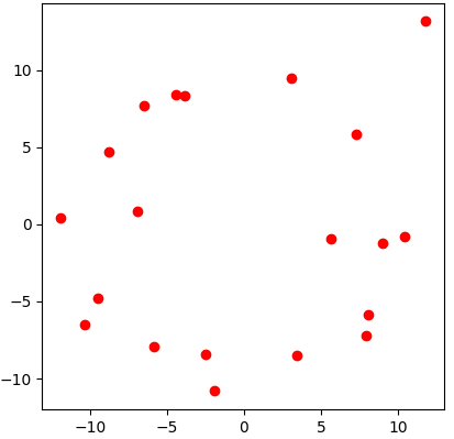
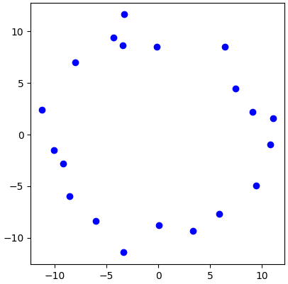
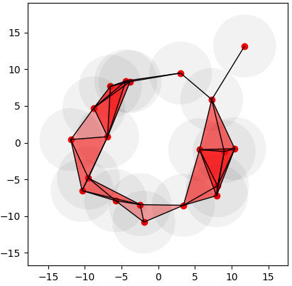
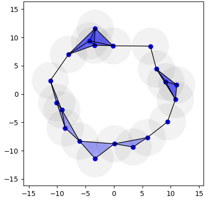
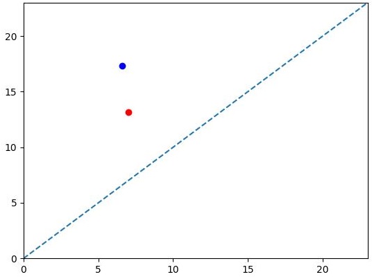
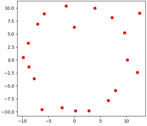
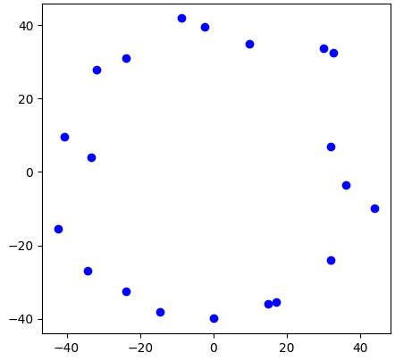
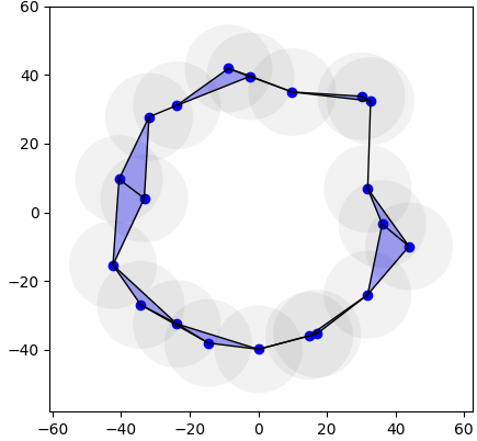
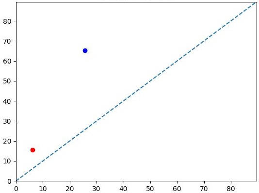
Figure 1: Two pairs of point clouds, one without scaling (top row) and another with a large amount of scaling (bottom row), and their 1D persistence diagrams ($\displaystyle H_{1}$). The red and blue point clouds in the top row (first two figures) are both sampled from noisy circles in the $\displaystyle[-10,10]\times[-10,10]$ box. The third and fourth figures show the births of the hole in each case at diameters of around $\displaystyle 7$. The first (red) point cloud in the bottom row is similar to the ones in the top row, but the second (blue) point cloud is sampled from a noisy circle in the $\displaystyle[-80,80]\times[-80,80]$ box. Its hole feature is born at a diameter of around $\displaystyle 26$. The bottleneck distance between the pair of PDs is small in the top row, but can be quite large depending on the degree of scaling of the second (blue) point cloud in the bottom row.

While such scalings may have to be handled explicitly in certain applications, they often show up as a natural result of algorithmic pipelines that transforms the first PCD into the second. In fact, this is a typical scenario when the second PCD is produced by applying dimension reduction (DR) to the first PCD. For a direct illustration, see Figure 2 (in Page 2) to observe how UMAP [15], a popular nonlinear DR method applied under default settings, shrinks a 3D loop forming a saddle boundary in a $\displaystyle 200\times 200\times 100$ box to nearly a unit circle in the 2D plane. While the topology of the saddle boundary is clearly preserved by the UMAP reduction by capturing its loop structure, standard bottleneck distance between the PDs of the input and the output representations cannot be constrained by any reasonably small bound.

We consider the following motivating questions: Can we define a scale-invariant bottleneck distance between PDs? Can we derive tighter stability bounds on this distance than ones known for the standard bottleneck distance? And can we use this new distance and associated stability bounds to capture how well standard DR techniques may preserve homology?

1.1 Our Contributions

We define a new scale-invariant distance between persistence diagrams termed normalized bottleneck distance, $\displaystyle\operatorname{d_{N}}$, and study its properties (see Definition 2.5). On top of being scale-invariant (see Theorem 2.6), $\displaystyle\operatorname{d_{N}}$ is a pseudometric for persistence diagrams, and also has the computational advantage of not needing to directly compute an optimal scaling/dilation factor. In defining $\displaystyle\operatorname{d_{N}}$, we also develop a broader framework called metric decomposition for comparing finite metric spaces of equal cardinality that also have a bijection defined between them. We utilize this metric decomposition to prove a stability result for $\displaystyle\operatorname{d_{N}}$ (we write $\displaystyle\operatorname{d_{N}}(X,Y)$ in short for $\displaystyle\operatorname{d_{N}}(\operatorname{dgm}(X),\operatorname{dgm}(Y))$ and similarly for $\displaystyle\operatorname{d_{B}}$):

Theorem 2.10.

$\displaystyle\operatorname{d_{N}}(X,Y)\leq\frac{2\left\lVert\Delta\right\rVert}{\operatorname{diam}(Y)}\,$,

where $\displaystyle\Delta$ represents the optimal metric decomposition of $\displaystyle Y$ in terms of $\displaystyle X$ for finite metric spaces $\displaystyle X,Y$ of same cardinality with a bijection between them (see Definition 2.7) and $\displaystyle\operatorname{diam}(Y)$ is the diameter of $\displaystyle Y$. We derive this stability result by explicitly bounding the distortion of the associated bijective map, and hence the Gromov-Hausdorff distance between $\displaystyle X$ and $\displaystyle Y$ (see Theorem 1.7 and Definition 1.9).

We then study two popular dimension reduction techniques, Johnson-Lindenstrauss (JL) projections and metric multidimensional scaling (mMDS), and a third class of general biLipschitz mappings. We provide new bounds on how well these dimension reduction techniques preserve homology with respect to $\displaystyle\operatorname{d_{N}}$. For a JL map $\displaystyle f$ taking input $\displaystyle X$ to $\displaystyle f(X)$, we derive the following new bounds on $\displaystyle\operatorname{d_{B}}$ and $\displaystyle\operatorname{d_{N}}$:

Theorem 3.3.

$\displaystyle\operatorname{d_{B}}(X,f(X))<\epsilon\operatorname{diam}(X)\,$

and

Corollary 1.3.

$\displaystyle\operatorname{d_{N}}(X,f(X))<\epsilon$ ,

where $\displaystyle 0<\epsilon<1$ is the tolerance up to which pairwise distances are preserved by $\displaystyle f$ (see Equation (2) for the formal definition). For mMDS, we present new bounds for both $\displaystyle\operatorname{d_{B}}$ and $\displaystyle\operatorname{d_{N}}$ between persistence diagrams of $\displaystyle X$ and its projection in terms of the eigenvalues of the covariance matrix:

Corollary 1.4.

$\displaystyle\displaystyle\operatorname{d_{B}}(X,P_{X}^{(m)}(X))\leq\sqrt{2}\sqrt[4]{\sum\limits_{m+1}^{d}\lambda_{i}^{2}}$,

and

Corollary 1.5.

$\displaystyle\operatorname{d_{N}}(X,P^{(m)}_{X}(X))\leq\frac{2\sqrt{2}}{\operatorname{diam}(P^{(m)}_{X}(X))}\sqrt[4]{\frac{\left(\sum\limits_{i=1}^{m}\lambda_{i}^{2}\right)\left(\sum\limits_{i=m+1}^{d}\lambda_{i}^{2}\right)}{\left(\sum\limits_{i=1}^{d}\lambda_{i}^{2}\right)}}$ ,

where $\displaystyle P_{X}^{(m)}:X\rightarrow\mathbb{R}^{m}$ is the mMDS projection (see Definition 3.5) and $\displaystyle\lambda_{i}$’s are the eigenvalues of the covariance matrix. These bounds indicate that if the first $\displaystyle m$ eigenvectors capture most of the variance, and hence the remaining eigenvalues $\displaystyle\{\lambda_{i}\}_{m+1}^{d}$ are small, then homology is preserved well in terms of small values of both $\displaystyle\operatorname{d_{B}}$ and $\displaystyle\operatorname{d_{N}}$. And finally, we study a general class of $\displaystyle k$-biLipschitz projection maps $\displaystyle f:X\rightarrow Y$, i.e., which satisfy $\displaystyle(1/k)\,d_{X}\,\leq d_{Y}\leq\,k\,d_{X}$ for some $\displaystyle k\geq 1$, to obtain bounds on homology preservation in terms of $\displaystyle\operatorname{d_{N}}$ as

Corollary 1.6.

$\displaystyle\displaystyle\operatorname{d_{N}}{(X,Y)}\leq\left|\frac{k^{2}-1}{k}\right|\frac{\operatorname{diam}(X)}{\operatorname{diam}(Y)}$ .

1.2 Related Work

The use of bottleneck distance between persistence diagrams as a means of measuring similarity between metric spaces has gained much attention in the recent years. In 2014, Chazal et al. [6] showed that the bottleneck distance between PDs of PCD is indeed stable with respect to the input metric spaces:

Theorem 1.7 (Chazal et al., 2014 [6]).

$\displaystyle\operatorname{d_{B}}(X,Y)\leq 2\operatorname{d_{GH}}(X,Y)$,

where $\displaystyle\operatorname{d_{GH}}$ is the Gromov-Hausdorff distance (see Definition 1.9). Some researchers have recently considered modifications of the standard bottleneck distance between PDs that are invariant to certain transformations of the input metric spaces. Sheehy et al. [4] studied a shift-invariant bottleneck distance between two PDs $\displaystyle A,B$ defined as

$$\operatorname{d}_{\mathrm{sB}}(A,B)=\min_{s\in\mathbb{R}}\operatorname{d_{B}}\left(A_{s},B\right)\text{ where }A_{s}=\{s+a\ |\ a\in A\}.$$

While shifts of PDs in the above manner will not directly capture scalings of the metric spaces, the authors mentioned that this shift-invariant similarity measure could possibly be applied to log-scale persistence diagrams in order to define a scale-invariant bottleneck distance. At the same time, the question of scale invariance was not directly considered. Cao et al. [2] were the first to study a dilation (i.e., scale) invariant bottleneck distance, where they defined the dissimilarity measure

$$\overline{\mathrm{d}_{\rm D}}\left(X,Y\right)=\inf_{c\in\mathbb{R}_{+}}\operatorname{d_{B}}\left(cX,Y\right)\,.$$ (1)

They show that this similarity measure is in fact dilation invariant and stable with respect to the Gromov-Hausdorff distance. They further provide computational results for efficient searching for an optimal scaling factor $\displaystyle c$, as well as provide some computational evidence for the efficacy of this similarity measure. On the other hand, we prove that an optimal decomposition of $\displaystyle Y$ in terms of $\displaystyle X$ always exists in our case (see Theorem 2.9).

The question of preservation of topology of PCD under Johnson-Lindenstrauss (JL) random projections was addressed by Sheehy [16] and Lotz [13]. They both showed that Čech persistent homology of a PCD is approximately preserved under JL random projections up to a $\displaystyle(1\pm\epsilon)$ multiplicative factor for any $\displaystyle\epsilon\in[0,1]$ [16, 13]. Sheehy proved this result for a PCD with $\displaystyle n$ points, whereas the result of Lotz considered more general sets of bounded Gaussian width, and also implied dimensionality reductions for sets of bounded doubling dimension in terms of the spread (ratio of the maximum to minimum interpoint distance). Our bound of $\displaystyle\epsilon$ on $\displaystyle\operatorname{d_{N}}$ in Corollary 3.4 agrees with these results, while our proof approaches are distinct since we obtain a new bound on the distortion (see Definition 1.8) of the JL map in order to derive our bound. Recently, the results of Sheehy and Lotz were extended by Arya et al. [1] to the case of more general $\displaystyle k$-distances. Similar bounds on homology preservation under other nonlinear DR techniques such as multidimensional scaling have been scarce.

A motivation for our study of homology preservation under $\displaystyle k$-biLipschitz maps was the work of Mahabadi et al. [14] who introduced the notion of outer biLipschitz extensions of maps between Euclidean spaces as a means for nonlinear dimension reduction. But homology preservation was not a focus of their work.

The related problem of combining TDA with DR to design new topology-preserving DR techniques has been studied as well. Motivated by the nonlinear DR technique of Isomap [17], Yan et al. [20] proposed a method for homology-preserving DR via manifold landmarking and tearing. Wagner et al. [19] have used a topological loss term in a gradient-descent based method for DR that outperformed standard DR techniques in topology preservation. But our focus is on quantifying topology preservation of existing DR techniques.

1.3 Notation and Definitions

We focus on comparing finite metric spaces denoted as $\displaystyle(X,d_{X})$ and $\displaystyle(Y,d_{y})$ unless otherwise stated, and neither $\displaystyle X$ nor $\displaystyle Y$ are trivial ($\displaystyle d_{X}$ and $\displaystyle d_{Y}$ are not identically $\displaystyle 0$). The size of a metric space is measured by its diameter, $\displaystyle\operatorname{diam}(X)=\max\limits_{a,b\in X}d_{X}(a,b)$.

A common metric for comparing metric spaces is the Gromov-Hausdorff distance ($\displaystyle\operatorname{d_{GH}}$), which can be thought of as a way of measuring to what degree two spaces are isometric. We first define distortion, and define $\displaystyle\operatorname{d_{GH}}$ in terms of distortion.

Definition 1.8.

The distortion of a relation $\displaystyle\sigma\in\mathcal{R}(X,Y)$ between metric spaces $\displaystyle X$ and $\displaystyle Y$ is

$$\operatorname{dis}\sigma=\sup\left\{|d(x,x^{\prime})-d(y,y^{\prime})|:(x,y),\left(x^{\prime},y^{\prime}\right)\in\sigma\right\}\,.$$

The distortion of a mapping $\displaystyle f:X\rightarrow Y$, dis($\displaystyle f$), is the distortion of the graph of $\displaystyle f$.

Definition 1.9.

The Gromov-Hausdorff distance between metric spaces $\displaystyle X$ and $\displaystyle Y$ is

$$\operatorname{d_{GH}}(X,Y)=\frac{1}{2}\inf\{\operatorname{dis}R:R\in\mathcal{R}(X,Y)\}\,.$$

We denote by $\displaystyle\operatorname{dgm}(X)$ the Vietoris-Rips persistence diagram of metric space $\displaystyle X$. For a finite metric space $\displaystyle X$, this diagram consists of a finite multiset of points above the diagonal, i.e., $\displaystyle y=x$ line, in the extended plane $\displaystyle\bar{\mathbb{R}}^{2}$. To this finite multiset, we add the infinitely many points on the diagonal, each with infinite multiplicity. We now list the standard definition of the bottleneck distance between two such PDs [10, §VIII].

Definition 1.10.

The bottleneck distance between the persistence diagrams of two finite metric spaces $\displaystyle X$ and $\displaystyle Y$ is

$$\operatorname{d_{B}}(\operatorname{dgm}(X),\operatorname{dgm}(Y))=\min_{\gamma:\operatorname{dgm}{X}\to\operatorname{dgm}{Y}}\max_{x\in\operatorname{dgm}{X}}\left\lVert x-\gamma(x)\right\rVert_{\infty}~{}\text{for a bijection }\gamma.$$

We shorten the notation to $\displaystyle\operatorname{d_{B}}(X,Y)$ when there is no ambiguity.

Finally, we collect in Table 1 some of the notation used throughout this paper.

Table 1: Notation used throughout the paper, and their description.

$\displaystyle\textnormal{VR}(X,r)$	The Vietoris-Rips complex of metric space $\displaystyle X$ at diameter $\displaystyle r$
$\displaystyle\operatorname{dgm}(X)$	The Vietoris-Rips persistence diagram of metric space $\displaystyle X$
$\displaystyle\operatorname{d_{B}}(X,Y)$	Bottleneck distance between $\displaystyle\operatorname{dgm}(X)$ and $\displaystyle\operatorname{dgm}(Y)$
$\displaystyle\operatorname{diam}_{X}(A)$	The diameter of a set $\displaystyle A\subset X$ with respect to a metric $\displaystyle d_{X}$, $\displaystyle\max\limits_{a,b\in A}\{d_{X}(a,b)\}$
$\displaystyle s\cdot A$	$\displaystyle\{s\cdot a\ |\ a\in A\}$ when $\displaystyle A\subset\mathbb{R}^{n}$
$\displaystyle C(Z)$	The covariance matrix $\displaystyle ZZ^{T}$ of $\displaystyle Z$, when $\displaystyle Z=[z_{1}\dots\ z_{n}]$ is a data matrix
$\displaystyle A\circ B$	The Hadamard product of $\displaystyle A$ and $\displaystyle B$
$\displaystyle\displaystyle A^{\circ^{n}}$	The $\displaystyle n^{\text{th}}$ Hadamard power of a matrix $\displaystyle A$
$\displaystyle G_{X}$	The gram matrix of a data set $\displaystyle X\subset\mathbb{R}^{n}$
$\displaystyle I_{|_{m}}$	The matrix: $\displaystyle\operatorname{diag}(\underbrace{1,1,\ldots,1}_{m},\underbrace{0,0,\ldots,0}_{n-m})$ for $\displaystyle m\leq n$
$\displaystyle\Sigma_{|_{m}}$	The matrix $\displaystyle\Sigma\cdot I_{|_{m}}$

2 Methods and Results

Given a metric space $\displaystyle(X,d_{X})$ we consider the family of metric spaces $\displaystyle sX:=(X,sd_{X})$ for $\displaystyle s>0$. In words, we consider a family of metrics on $\displaystyle X$ that are positive scalars of $\displaystyle d_{X}$. Intuitively, the family $\displaystyle sX$ can be thought of as all dilations and contractions of $\displaystyle X$.

Proposition 2.1.

The following properties hold for a metric space $\displaystyle(X,d_{X})$ and $\displaystyle p,q>0$.

1. $\displaystyle\operatorname{diam}(pX)=p\operatorname{diam}(X)$.

2. $\displaystyle p(qX)=(pq)X$.

Scaling metric spaces has natural consequences on VR complexes, persistence diagrams, and bottleneck distances.

Lemma 2.2.

Let $\displaystyle s>0$. Then $\displaystyle\operatorname{VR}(X,r)=\operatorname{VR}(sX,sr)$ for all $\displaystyle r>0$.

Proof.

Let $\displaystyle s,r>0$. By definition, $\displaystyle\operatorname{VR}(X,r)=\{\sigma\subset X\ |\ \operatorname{diam}_{X}(\sigma)<r\}$, so let $\displaystyle\sigma\in\operatorname{VR}(X,r)$. Then $\displaystyle\operatorname{diam}_{X}(\sigma)<r\iff s\operatorname{diam}_{X}(\sigma)<sr\iff\operatorname{diam}_{X}(s\sigma)<sr\iff\operatorname{diam}_{sX}(\sigma)<sr\iff\sigma\in\operatorname{VR}(sX,sr)$. ∎

Corollary 2.3.

$\displaystyle s\cdot\operatorname{dgm}(X)=\operatorname{dgm}(sX)$ for all $\displaystyle s>0$.

Proof.

Follows immediately from Lemma 2.2. ∎

Theorem 2.4.

$\displaystyle s\cdot\operatorname{d_{B}}(X,Y)=\operatorname{d_{B}}(sX,sY)$ for all $\displaystyle s>0$.

Proof.

$$s\cdot\operatorname{d_{B}}(X,Y) =s\left[\min\limits_{\gamma:\operatorname{dgm}(X)\rightarrow\operatorname{dgm}(Y)}\,\max\limits_{x\in\operatorname{dgm}(X)}\,\left\lVert x-\gamma(x)\right\rVert\right]$$

$$=\min\limits_{\gamma:\operatorname{dgm}(X)\rightarrow\operatorname{dgm}(Y)}\,\max\limits_{x\in\operatorname{dgm}(X)}\,s\left\lVert x-\gamma(x)\right\rVert$$

$$=\min\limits_{\gamma:\operatorname{dgm}(X)\rightarrow\operatorname{dgm}(Y)}\,\max\limits_{x\in\operatorname{dgm}(X)}\,\left\lVert sx-s\gamma(x)\right\rVert.$$

Applying Corollary 2.3, we have that $\displaystyle sx\in\operatorname{dgm}(sX)$ and $\displaystyle s\gamma(x)\in\operatorname{dgm}(sY)$, and hence the

above expression $\displaystyle=\displaystyle\min\limits_{\gamma:\operatorname{dgm}(sX)\rightarrow\operatorname{dgm}(sY)}\,\max\limits_{x\in\operatorname{dgm}(sX)}\left\lVert x-\gamma(x)\right\rVert=\operatorname{d_{B}}(sX,sY)$ by definition. ∎

We define the normalized bottleneck distance using the notion of metric scaling.

Definition 2.5 (Normalized Bottleneck).

$\displaystyle\displaystyle\operatorname{d_{N}}(X,Y)=\operatorname{d_{B}}\left(\frac{X}{\operatorname{diam}(X)},\frac{Y}{\operatorname{diam}(Y)}\right)$.

It is easy to see that $\displaystyle\operatorname{d_{N}}$ is indeed a pseudometric on persistence diagrams. It inherits most properties of $\displaystyle\operatorname{d_{B}}$, except it is possible for $\displaystyle\operatorname{d_{N}}$ to be zero for two distinct PDs. We can see that $\displaystyle\operatorname{d_{N}}$ fails the identity of indiscernibles by taking a metric space $\displaystyle X$ and scaled version $\displaystyle sX$ for $\displaystyle s>0$. Then $\displaystyle\operatorname{d_{N}}(sX,X)=\operatorname{d_{N}}(X,X)=0$, despite $\displaystyle sX$ and $\displaystyle X$ being distinct for $\displaystyle s\neq 1$.

Theorem 2.6 (Scale-invariance).

$\displaystyle\displaystyle\operatorname{d_{N}}(pX,qY)=\operatorname{d_{N}}(X,Y)$ for all $\displaystyle p,q>0$.

Proof.

Let $\displaystyle p,q>0$. Then

$$\operatorname{d_{N}}(pX,qY) =\operatorname{d_{B}}\left(\frac{pX}{\operatorname{diam}(pX)},\frac{qY}{\operatorname{diam}(qY)}\right)$$

$$=\operatorname{d_{B}}\left(\frac{p}{p}\frac{X}{\operatorname{diam}(X)},\frac{q}{q}\frac{Y}{\operatorname{diam}(Y)}\right)$$

$$=\operatorname{d_{B}}\left(\frac{X}{\operatorname{diam}(X)},\frac{Y}{\operatorname{diam}(Y)}\right)$$

$$=\operatorname{d_{N}}(X,Y).$$

∎

2.1 Metric Decomposition

When $\displaystyle X$ and $\displaystyle Y$ are of equal size and we have a bijection $\displaystyle f:X\rightarrow Y$, we can examine the metrics of both $\displaystyle X$ and $\displaystyle Y$ via distance matrices $\displaystyle D_{X}$ and $\displaystyle D_{Y}$, where $\displaystyle[D_{X}]_{ij}:=d_{X}(x_{i},x_{j})$ and $\displaystyle[D_{Y}]_{ij}:=d_{Y}(f(x_{i}),f(x_{j}))$. This is a typical setting encountered in dimension reduction where $\displaystyle Y$ is a lower dimensional projection of $\displaystyle X$. Note that we must have such a map $\displaystyle f$ to compare $\displaystyle D_{X}$ and $\displaystyle D_{Y}$, since distance matrices are only unique up to orderings of the points. We have that $\displaystyle\operatorname{diam}(X)=\left\lVert D_{X}\right\rVert_{\max}$. We omit the subscript and write $\displaystyle\left\lVert\cdot\right\rVert$ to mean $\displaystyle\left\lVert\cdot\right\rVert_{\max}$ when it is clear.

Definition 2.7.

Let $\displaystyle f:X\rightarrow Y$ be a bijection, $\displaystyle s\geq 0$. Define $\displaystyle\Delta_{s}=\left[\delta_{ij}\right]_{s}=D_{Y}-sD_{X}$. We say that $\displaystyle sD_{X}+\Delta_{s}=D_{Y}$ is a metric decomposition of $\displaystyle Y$ in terms of $\displaystyle X$.

There are infinitely many choices for $\displaystyle s$ and hence infinitely many decompositions, so naturally we seek an optimal decomposition. Thinking about $\displaystyle\Delta_{s}$ as the “error” between $\displaystyle D_{X}$ and $\displaystyle D_{Y}$, we seek to minimize this error. In other words, we seek an $\displaystyle s$ such that $\displaystyle\left\lVert\Delta_{s}\right\rVert_{\max}$ is minimized. It is not immediately clear that such a scalar $\displaystyle s$ exists, but indeed this is a well-posed problem.

Lemma 2.8.

Let $\displaystyle X,Y$ be metric spaces, $\displaystyle f:X\rightarrow Y$ bijective, and let $\displaystyle h:\mathbb{R}_{+}\rightarrow\mathbb{R}$ be the map $\displaystyle s\mapsto\left\lVert\Delta_{s}\right\rVert_{\max}$. The following properties hold:

1. $\displaystyle h$ is continuous;

2. there exists an $\displaystyle m>0$ such that $\displaystyle h$ is strictly increasing on $\displaystyle[m,\infty)$.

Proof.

1. This follows from the continuity of $\displaystyle\left\lVert\cdot\right\rVert_{\max}$. Let $\displaystyle\epsilon>0$, and set $\displaystyle\displaystyle\delta=\frac{\epsilon}{\left\lVert D_{X}\right\rVert_{\max}}$. Then, if $\displaystyle|s-a|<\delta$, we have

   $$|h(s)-h(a)| =\left|\,\left\lVert\Delta_{s}\right\rVert_{\max}-\left\lVert\Delta_{a}\right\rVert_{\max}\,\right|$$

   $$=\left|\,\left\lVert D_{Y}-sD_{X}\right\rVert-\left\lVert D_{Y}-aD_{X}\right\rVert\,\right|.$$

   Applying the reverse triangle inequality, we obtain

   $$|h(s)-h(a)| \leq\left\lVert(s-a)D_{X}\right\rVert$$

   $$=|s-a|\left\lVert D_{X}\right\rVert$$

   $$<\delta\left\lVert D_{X}\right\rVert$$

   $$=\frac{\epsilon}{\left\lVert D_{X}\right\rVert_{\max}}\left\lVert D_{X}\right\rVert_{\max}~{}=\epsilon\,.$$

2. Let $\displaystyle m>0$ be such that $\displaystyle md_{X}(a,b)-d_{Y}(f(a),f(b))>0$ for all $\displaystyle a,b\in X$, and let $\displaystyle u,v\in X$ achieve the maximum $\displaystyle md_{X}(u,v)-d_{Y}(f(u),f(v))=\max\limits_{a,b}\{md_{X}(a,b)-d_{Y}(f(a),f(b))\}=\left\lVert\Delta_{m}\right\rVert_{\max}$. If $\displaystyle p>q\geq m$, then clearly $\displaystyle u,v$ also achieve the maximums for $\displaystyle\left\lVert\Delta_{p}\right\rVert_{\max}$ and $\displaystyle\left\lVert\Delta_{q}\right\rVert_{\max}$, so necessarily

   $$h(p)-h(q) =\left\lVert\Delta_{p}\right\rVert_{\max}-\left\lVert\Delta_{q}\right\rVert_{\max}$$

   $$=p\cdot d_{X}(u,v)-d_{Y}(f(u),f(v))-(q\cdot d_{X}(u,v)-d_{Y}(f(u),f(v)))$$

   $$=(p-q)d_{X}(u,v)>0~{}\text{ since }p-q>0\,.$$

   Thus, $\displaystyle h(p)-h(q)>0$.

∎

Theorem 2.9.

Let $\displaystyle\displaystyle D_{Y}=sD_{X}+\Delta_{s}$ for any $\displaystyle s>0$. Then $\displaystyle\min\limits_{s}\left\lVert\Delta_{s}\right\rVert_{\max}$ exists.

Proof.

Let $\displaystyle h:\mathbb{R}_{+}\rightarrow\mathbb{R}$ be the mapping from Lemma 2.8. Using Property 2 in Lemma 2.8, let $\displaystyle m$ be a marker such that $\displaystyle h$ is strictly increasing on $\displaystyle[m,\infty)$. Then clearly $\displaystyle\displaystyle{\left.\kern-1.2pth\vphantom{\big{|}}\right|_{[m,\infty)}}$ has a global minimum at $\displaystyle m$. Likewise, $\displaystyle\displaystyle{\left.\kern-1.2pth\vphantom{\big{|}}\right|_{[0,m]}}$ has a global minimum since $\displaystyle h$ is continuous and $\displaystyle[0,m]$ is compact. Now, since $\displaystyle\mathbb{R}_{+}=[0,m]\cup[m,\infty)$ and $\displaystyle h$ achieves a minimum of both intervals, $\displaystyle h$ has global minimum $\displaystyle\displaystyle\min\{\min{\left.\kern-1.2pth\vphantom{\big{|}}\right|_{[m,\infty)}},\ \min{\left.\kern-1.2pth\vphantom{\big{|}}\right|_{[0,m]}}\}$. ∎

Hence we can always minimize $\displaystyle\left\lVert\Delta_{s}\right\rVert_{\max}$. In general, we let $\displaystyle s^{*}=\operatorname*{arg\,min}\limits_{s}\left\lVert\Delta_{s}\right\rVert_{\max}$ be an optimal decomposition of $\displaystyle Y$ in terms of $\displaystyle X$, and write $\displaystyle\Delta_{s^{*}}=\Delta$.

2.2 Stability Result

Since $\displaystyle\operatorname{d_{N}}$ and $\displaystyle\operatorname{d_{B}}$ are similarity measures on metric spaces that measure the spaces indirectly via their respective persistence diagrams, one would desire that $\displaystyle\operatorname{d_{N}}$ and $\displaystyle\operatorname{d_{B}}$ are “stable” with respect to the input metric spaces. Stability in this sense means that

• “small changes” to $\displaystyle X$ or $\displaystyle Y$ result in “small changes” to $\displaystyle\operatorname{d_{B}}$ and $\displaystyle\operatorname{d_{N}}$, and

• if $\displaystyle X$ and $\displaystyle Y$ are “close”, then $\displaystyle\operatorname{d_{N}}$ and $\displaystyle\operatorname{d_{B}}$ are also “close”.

To make these notions precise, small changes in $\displaystyle X$ or $\displaystyle Y$ and the closeness of $\displaystyle X$ and $\displaystyle Y$ are measured using some other metric for $\displaystyle X$ and $\displaystyle Y$, preferably one that compares the metric spaces directly. A good choice for this metric is the Gromov-Hausdorff distance, $\displaystyle\operatorname{d_{GH}}$, specified in Definition 1.9, Recall the bound on $\displaystyle\operatorname{d_{B}}$ in terms of $\displaystyle\operatorname{d_{GH}}$ given by Chazal et al. [6] in Theorem 1.7: $\displaystyle\operatorname{d_{B}}(X,Y)\leq 2\operatorname{d_{GH}}(X,Y)$. When we have a bijective correspondence between $\displaystyle X$ and $\displaystyle Y$ and hence a metric decomposition, we obtain a much stronger stability bound.

Theorem 2.10.

$$\operatorname{d_{N}}(X,Y)\leq\frac{2\left\lVert\Delta\right\rVert}{\operatorname{diam}(Y)}\,.$$

Proof.

Let $\displaystyle\displaystyle f:X\rightarrow Y$ be the bijection and $\displaystyle\displaystyle\hat{f}:\frac{X}{\left\lVert D_{X}\right\rVert}\rightarrow\frac{Y}{\left\lVert D_{Y}\right\rVert}$. Observe that

$$\operatorname{d_{N}}(X,Y)=\operatorname{d_{B}}\left(\frac{X}{\left\lVert D_{X}\right\rVert},\frac{Y}{\left\lVert D_{Y}\right\rVert}\right)\leq\operatorname{dis}(\hat{f})\,.$$

Using our decomposition,

$$\operatorname{dis}(\hat{f}) =\max\limits_{a,b\in X}\left|\frac{d_{X}(a,b)}{\left\lVert D_{X}\right\rVert}-\frac{sd_{X}(a,b)+\delta_{s}(a,b)}{\left\lVert D_{Y}\right\rVert}\right|$$

$$=\max\limits_{a,b\in X}\frac{\big{|}d_{X}(a,b)\left\lVert sD_{X}+\Delta_{s}\right\rVert-\left\lVert D_{X}\right\rVert(sd_{X}(a,b)+\delta_{s}(a,b))\big{|}}{\left\lVert D_{X}\right\rVert\left\lVert D_{Y}\right\rVert}$$

$$=\max\limits_{a,b\in X}\frac{\big{|}(\left\lVert sD_{X}+\Delta_{s}\right\rVert-\left\lVert sD_{X}\right\rVert)d_{X}(a,b)-\left\lVert D_{X}\right\rVert\delta_{s}(a,b)\big{|}}{\left\lVert D_{X}\right\rVert\left\lVert D_{Y}\right\rVert}$$

$$\leq\max\limits_{a,b\in X}\frac{\big{|}\left\lVert sD_{X}+\Delta_{s}\right\rVert-\left\lVert sD_{X}\right\rVert\big{|}d_{X}(a,b)+\left\lVert D_{X}\right\rVert|\delta_{s}(a,b)|}{\left\lVert D_{X}\right\rVert\left\lVert D_{Y}\right\rVert}~{}~{}\text{ by triangle inequality.}$$

Observe that $\displaystyle\big{|}\left\lVert sD_{X}+\Delta_{s}\right\rVert-\left\lVert sD_{X}\right\rVert\big{|}\leq\left\lVert\Delta_{s}\right\rVert$ via the reverse triangle inequality, so,

$$\operatorname{d_{N}}(X,Y) \leq\max\limits_{a,b\in X}\frac{\left\lVert\Delta_{s}\right\rVert d_{X}(a,b)+\left\lVert D_{X}\right\rVert|\delta_{s}(a,b)|}{\left\lVert D_{X}\right\rVert\left\lVert D_{Y}\right\rVert}$$

$$\leq\max\limits_{a,b\in X}\frac{2\left\lVert\Delta_{s}\right\rVert\left\lVert D_{X}\right\rVert}{\left\lVert D_{X}\right\rVert\left\lVert D_{Y}\right\rVert}$$

$$=2\frac{\left\lVert\Delta_{s}\right\rVert}{\left\lVert D_{Y}\right\rVert}\,.$$

This holds for all $\displaystyle s$, and thus holds when $\displaystyle\Delta_{s}=\Delta$. ∎

3 Applications in Dimension Reduction

Dimension reduction (DR) techniques are used ubiquitously and are paramount for discovering latent features of data and visualizing high-dimensional data. However, the curse of dimensionality dictates that distances tend to grow as the number of dimension grow, which can lead to a proportionate amount of scaling under certain DR techniques. But more specifically in our context, DR techniques are necessarily bijective between its respective metric spaces, and thus exhibit metric decompositions. Hence we seek to derive guarantees for homology preservation under DR in terms of bounds on $\displaystyle\operatorname{d_{N}}$ between the PDs of the input and reduced metric spaces. We look at two specific dimension reduction techniques, Johnson-Lindenstrauss projections and metric multidimensional scaling, and provide specific bounds for $\displaystyle d_{B}$ and $\displaystyle d_{N}$. We also provide a more general condition for biLipschitz functions that may serve other dimension reduction techniques.

3.1 Johnson-Lindenstrauss Linear Projection

A Johnson-Lindenstrauss (JL) linear projection [12] is, for some $\displaystyle 0<\epsilon<1$, a linear map $\displaystyle f:X\rightarrow Y$ satisfying the inequality

$$(1-\epsilon)d_{X}(u,v)^{2}\leq d_{Y}(f(u),f(v))^{2}\leq(1+\epsilon)d_{X}(u,v)^{2}\text{ for all }u,v\in X\,.$$ (2)

A mapping that satisfies this property may be desirable in many cases, as it guarantees pairwise distances do not change “too much” under $\displaystyle f$. Such a mapping is guaranteed to exist from $\displaystyle\mathbb{R}^{N}$ to $\displaystyle\mathbb{R}^{n}$ for $\displaystyle n\leq N$ provided $\displaystyle n$ is not too small. This result was formalized in the classical Johnson-Lindenstrauss Lemma.

Lemma 3.1 (Johnson and Lindenstrauss, 1984 [12]).

Given $\displaystyle 0<\epsilon<1$, a set $\displaystyle X$ of $\displaystyle m$ points in $\displaystyle\mathbb{R}^{N}$, and a number $\displaystyle n>8\ln(m)/\epsilon^{2}$, there is a linear map $\displaystyle f:\mathbb{R}^{N}\rightarrow\mathbb{R}^{n}$ such that

$$(1-\epsilon)\|u-v\|^{2}\leq\|f(u)-f(v)\|^{2}\leq(1+\epsilon)\|u-v\|^{2}~{}\text{ for all }u,v\in X\,.$$

Because pairwise distances under a $\displaystyle\mathrm{JL}$ mapping do not change too much, we might expect a small difference in persistence as well, i.e., a small bottleneck distance. However, this pairwise distance bound is multiplicative with respect to $\displaystyle d_{X}$, which leads to a potentially large bottleneck distance.

Lemma 3.2.

Let $\displaystyle\epsilon>0$. If $\displaystyle\displaystyle\left|\frac{\operatorname{d}(f(x),f(x^{\prime}))}{\operatorname{d}(x,x^{\prime})}-1\right|<\epsilon$ for all $\displaystyle x,x^{\prime}\in X$, then

$$\operatorname{dis}(f)<\epsilon\operatorname{diam}(X)\,.$$

Proof.

Let $\displaystyle x,x^{\prime}\in X$, where $\displaystyle(1-\epsilon)\operatorname{d}(x,x^{\prime})<d(f(x),f(x^{\prime}))<(1+\epsilon)\operatorname{d}(x,x^{\prime})$. Subtracting $\displaystyle\operatorname{d}(x,x^{\prime})$ gives

$$-\epsilon\operatorname{d}(x,x^{\prime})<d(f(x),f(x^{\prime}))-\operatorname{d}(x,x^{\prime})<\epsilon\operatorname{d}(x,x^{\prime})\,.$$

Hence $\displaystyle\left|\operatorname{d}(f(x),f(x^{\prime}))-\operatorname{d}(x,x^{\prime})\right|<\epsilon\operatorname{d}(x,x^{\prime})$. Taking the supremum over all $\displaystyle x,x^{\prime}\in X$ on both sides gives us our result. ∎

Theorem 3.3 (Johnson-Lindenstrauss Homology Preservation).

Let $\displaystyle X\subset\mathbb{R}^{N}$ with $\displaystyle|X|=m$, and let $\displaystyle\epsilon\in(0,1)$. If $\displaystyle f:\mathbb{R}^{N}\rightarrow\mathbb{R}^{n}$ is a JL-linear map ($\displaystyle n>8\ln(m)/\epsilon^{2}$), then

$$\operatorname{d_{B}}(X,f(X))<\epsilon\operatorname{diam}(X)\,.$$

Proof.

Let $\displaystyle 0<\epsilon<1$, and $\displaystyle f$ be a Johnson-Lindenstrauss projection with $\displaystyle n>8\ln(m)/\epsilon^{2}$. Then by the Johnson-Lindenstrauss lemma (Lemma 3.1), we have

$$(1-\epsilon)\|x-x^{\prime}\|^{2}\leq\|f(x)-f(x^{\prime})\|^{2}\leq(1+\epsilon)\|x-x^{\prime}\|^{2}\,.$$

Taking positive roots, we have

$$\sqrt{1-\epsilon}\|x-x^{\prime}\|\leq\|f(x)-f(x^{\prime})\|\leq\sqrt{1+\epsilon}\|x-x^{\prime}\|\,,$$

and since $\displaystyle 1-\epsilon<\sqrt{1-\epsilon}$ and $\displaystyle\sqrt{1+\epsilon}<1+\epsilon$, we arrive at

$$(1-\epsilon)\|x-x^{\prime}\|\leq\|f(x)-f(x^{\prime})\|\leq(1+\epsilon)\|x-x^{\prime}\|\,.$$

Hence, $\displaystyle\displaystyle\left|\frac{\|f(x)-f(x^{\prime})\|}{\|x-x^{\prime}\|}-1\right|<\epsilon$. Applying Lemma 3.2 gives us the desired result. ∎

We can see that the bound in Theorem 3.3 can be large when $\displaystyle\operatorname{diam}(X)$ is large. But this is not an issue with the normalized bottleneck since our spaces are normalized.

Corollary 3.4.

For a JL-Linear map, $\displaystyle\operatorname{d_{N}}(X,f(X))<\epsilon$ .

3.2 Metric Multidimensional Scaling

Metric multidimensional scaling (mMDS) is a generalization of the classical multidimensional scaling (MDS) [8]. We introduce the framework of mMDS, prove a new result on the projection map of mMDS (Lemma 3.7), and use it to derive new bounds on $\displaystyle\operatorname{d_{B}}$ and $\displaystyle\operatorname{d_{N}}$ between the input and output spaces of mMDS. The mMDS framework orthogonally projects data onto a subspace chosen to minimize mean-squared error or to maximize variance. More precisely, given an input metric space $\displaystyle X=(\{x_{1},\dots,x_{n}\},d_{X})$ and desired reduced dimension $\displaystyle m$, we find a centered data set $\displaystyle\tilde{X}=\{\tilde{x}_{1},\ldots,\tilde{x}_{n}\}\subset\mathbb{R}^{m}$ such that $\displaystyle\sum\limits_{i,j=1}^{n}(d(x_{i},x_{j})-\left\lVert\tilde{x_{i}}-\tilde{x}_{j}\right\rVert)^{2}$ is minimized. Such a projection can be achieved in two steps.

1. Obtain a realization $\displaystyle\Phi$ of $\displaystyle X$ in $\displaystyle\mathbb{R}^{k}$ for some $\displaystyle k$, i.e., $\displaystyle\Phi:X\rightarrow\Phi(X)\subset\mathbb{R}^{k}$ is an isometry.

2. Orthogonally project the realized data onto the first $\displaystyle m\leq d$ dominant eigenvectors of the covariance matrix $\displaystyle C(\Phi(X))$.

To find a realization of $\displaystyle X$ in $\displaystyle\mathbb{R}^{k}$, recall that $\displaystyle-\frac{1}{2}D_{X}^{\circ^{2}}=C_{n}G_{X}C_{n}$, where $\displaystyle G_{X}$ is the Gram matrix of $\displaystyle X$, and $\displaystyle C_{n}=I_{n}-\frac{1}{n}\mathbf{1}_{n}$ is the centering matrix. Since $\displaystyle G_{X}$ is positive semidefinite, it has a unique root $\displaystyle Z=[z_{1}\dots z_{n}]\in\mathbb{R}^{k\times n}$ so that $\displaystyle Z^{T}Z=G_{X}$, for some $\displaystyle k$. The realization of $\displaystyle X$ are the columns of $\displaystyle Z$, i.e., $\displaystyle\Phi(X)=\{z_{1},\dots,z_{n}\}$.

With our realization matrix $\displaystyle Z$ we can compute the singular-value decomposition $\displaystyle Z=U\Sigma V^{T}$, where we choose $\displaystyle\Sigma=\operatorname{diag}(\sigma_{1},\dots,\sigma_{n})$ with $\displaystyle\sigma_{1}\geq\ldots\geq\sigma_{n}$. The eigenvectors of $\displaystyle C(Z)=ZZ^{T}=U\Sigma^{2}U^{T}$ are precisely the columns of $\displaystyle U$, and the eigenvalues $\displaystyle\lambda_{i}$ of $\displaystyle C(Z)$ are precisely $\displaystyle\sigma_{i}^{2}$. Taking the first $\displaystyle m$ columns of $\displaystyle U$, we perform an orthogonal projection.

Definition 3.5 (metric multidimensional scaling (mMDS)).

Let $\displaystyle X=(\{x_{i}\},d_{X}),\ i=1,\dots,n$ be a metric space, $\displaystyle G_{X}=U\Sigma^{2}U^{T}$ the corresponding Gram matrix, and $\displaystyle Z=[z_{1}\cdots z_{n}]$ a realization of $\displaystyle X$ in $\displaystyle\mathbb{R}^{k}$ where $\displaystyle G_{X}=Z^{T}Z$. Let $\displaystyle 0<m\leq d$, and $\displaystyle\tilde{U}=\left[u_{1}\cdots u_{m}\right]$ be the truncated matrix consisting of the first $\displaystyle m$ dominant eigenvectors of $\displaystyle G_{X}$. The mMDS reduction $\displaystyle P_{X}^{(m)}:X\rightarrow\mathbb{R}^{m}$ is the map $\displaystyle P_{X}^{(m)}(x_{i})=\tilde{x_{i}}=\operatorname{proj}_{\operatorname{Im}(\tilde{U})}z_{i}$.

We assume that the realization $\displaystyle\Phi$ in Step 1 above is attainable, even if this computation may be hard (in fact, such a realization may not be guaranteed to exist in all cases). More generally, the problem of mMDS is NP-hard but good approximation algorithms have been proposed [9], and it is considered to work well in practice [8]. Our focus is on deriving bounds on homology preservation by mMDS with respect to $\displaystyle\operatorname{d_{B}}$ and $\displaystyle\operatorname{d_{N}}$.

Remark 3.6.

$\displaystyle P_{X}^{(m)}$ can equivalently be represented in matrix form as $\displaystyle P\in\mathbb{R}^{k\times k}$ so that $\displaystyle\tilde{x_{i}}=Pz_{i}$. The corresponding data matrix of the image $\displaystyle\displaystyle P_{X}^{(m)}(\{x_{i}\})$ is then $\displaystyle\tilde{X}:=[Pz_{1}\cdots Pz_{n}]=PZ$. In fact, it can be shown that $\displaystyle\displaystyle P=\tilde{U}(\tilde{U}^{T}\tilde{U})^{-1}\tilde{U}^{T}$.

Lemma 3.7.

Let $\displaystyle Z=U\Sigma V^{T}$ be the singular value decomposition (SVD) of $\displaystyle Z$. Then $\displaystyle P$ can be diagonalized as $\displaystyle P=UI_{|_{m}}U^{T}$, and $\displaystyle\tilde{X}=U\Sigma_{|_{m}}V^{T}$ (see Table 1 for $\displaystyle I_{|_{m}},\Sigma_{|_{m}}$ notation).

Proof.

Since $\displaystyle P$ orthogonally projects onto the image of the first $\displaystyle m$ dominant eigenvectors of $\displaystyle C(X)$, We necessarily have $\displaystyle Pu_{i}=u_{i}$ for $\displaystyle 0\leq i\leq m$ and $\displaystyle Pu_{i}=0$ for $\displaystyle m<i\leq d$. Thus $\displaystyle P$ and $\displaystyle C(X)$ share eigenvectors, and the spectrum of $\displaystyle P$ consists of $\displaystyle m$ ones and $\displaystyle d-m$ zeros. Thus, P is diagonalizable, and if we order the eigenvalues/eigenvectors in decreasing order, we have $\displaystyle P=UI_{|_{m}}U^{T}$. Now, if $\displaystyle X=U\Sigma V^{T}$, then $\displaystyle\tilde{X}=PX=(UI_{|_{m}}U^{T})(U\Sigma V^{T})=(UI_{|_{m}})(U^{T}U)(\Sigma V^{T})=U(I_{|_{m}}\Sigma)V^{T}=U\Sigma_{|_{m}}V^{T}$. ∎

Unlike JL mappings, mMDS minimizes a more global measure of pairwise distance

$$J:=\sum\limits_{i,j=1}^{n}(d(x_{i},x_{j})-\left\lVert\tilde{x_{i}}-\tilde{x_{j}}\right\rVert)^{2}\,.$$

The minimum $\displaystyle J$ is related directly to the eigenvalues of the covariance matrix $\displaystyle C(X)$:

$$\min\limits_{\tilde{X}\subset\mathbb{R}^{m}}J=\sum\limits_{i=m+1}^{d}\lambda_{i}^{2}\ .$$

We now show that a similar relationship holds for the distortion of $\displaystyle P^{(m)}_{X}$ that depends only on the eigenvalues of the covariance matrix.

Theorem 3.8.

$\displaystyle\displaystyle\operatorname{dis}(P_{X}^{(m)})\leq\sqrt{2}\sqrt[4]{\sum\limits_{m+1}^{d}\lambda_{i}^{2}}$ .

We first prove a result on Hadamard product $\displaystyle A\circ A$ of square matrices $\displaystyle A$ with themselves.

Lemma 3.9.

Let $\displaystyle A=[a_{ij}],B=[b_{ij}]\in\mathbb{R}^{n\times n}$ be square matrices with non-negative entries. Then $\displaystyle\left\lVert A-B\right\rVert_{\max}^{2}\leq\left\lVert A^{\circ^{2}}-B^{\circ^{2}}\right\rVert_{\max}$.

Proof.

$$\left\lVert A-B\right\rVert_{\max}^{2} =(\max|a_{ij}-b_{ij}|)^{2}$$

$$=\max|a_{ij}-b_{ij}|^{2}$$

$$\leq\max|a_{ij}-b_{ij}||a_{ij}+b_{ij}|$$

$$=\max|(a_{ij}-b_{ij})(a_{ij}+b_{ij})|$$

$$=\max|a_{ij}^{2}-b_{ij}^{2}|$$

$$=\left\lVert A^{\circ^{2}}-B^{\circ^{2}}\right\rVert_{\max}\,.$$

∎

Proof of Theorem 3.8.

We note that $\displaystyle\operatorname{dis}(P_{X}^{(m)})^{2}=\left\lVert D_{X}-D_{\tilde{X}}\right\rVert_{\max}^{2}=\left\lVert D_{Z}-D_{\tilde{X}}\right\rVert_{\max}^{2}$. Applying Lemma 3.9, we get $\displaystyle\operatorname{dis}(P_{X}^{(m)})^{2}\leq\left\lVert D_{Z}^{\circ^{2}}-D_{\tilde{X}}^{\circ^{2}}\right\rVert_{\max}$. Now, recall that Euclidean distance matrices and corresponding Gram matrices are related as $\displaystyle Z^{T}Z=-\frac{1}{2}C_{k}D_{Z}^{\circ^{2}}C_{k}$. Since $\displaystyle C_{k}$ is idempotent we can rearrange this so that $\displaystyle-\frac{1}{2}D_{Z}^{\circ^{2}}=C_{k}Z^{T}ZC_{k}=C_{k}V\Sigma^{2}V^{T}C_{k}=(C_{k}V)\Sigma^{2}(V^{T}C_{k}^{T})$. Now since $\displaystyle C_{k}$ and $\displaystyle V$ are both unitary, $\displaystyle Q:=C_{k}V$ is also unitary, so we can write $\displaystyle-\frac{1}{2}D_{Z}^{\circ^{2}}=Q\Sigma^{2}Q^{T}$. Using the same argument for $\displaystyle D_{\tilde{X}}^{\circ^{2}}$ and applying Lemma 3.7, we get $\displaystyle-\frac{1}{2}D_{\tilde{X}}^{\circ^{2}}=Q\Sigma_{|_{m}}^{2}Q^{T}$. So now,

$$\left\lVert D_{X}^{\circ^{2}}-D_{\tilde{X}}^{\circ^{2}}\right\rVert_{\max} =2\left\lVert Q\Sigma^{2}Q^{T}-Q\Sigma_{|_{m}}^{2}Q^{T}\right\rVert_{\max}$$

$$\leq 2\left\lVert Q\Sigma^{2}Q^{T}-Q\Sigma_{|_{m}}^{2}Q^{T}\right\rVert_{F}~{}~{}\text{(Frobenius norm)}$$

$$=2\left\lVert Q(\Sigma^{2}-\Sigma_{|_{m}}^{2})Q^{T}\right\rVert_{F}\,.$$

Since $\displaystyle\left\lVert\cdot\right\rVert_{F}$ is unitary invariant, the above expression is

$$=2\left\lVert\Sigma^{2}-\Sigma_{|_{m}}^{2}\right\rVert_{F}=2\sqrt{\sum\limits_{i=m+1}^{d}\lambda_{i}^{2}}\,.$$

Bringing everything together, we arrive at

$$\operatorname{dis}(P_{X}^{(m)})^{2}~{}\leq~{}2\sqrt{\sum\limits_{i=m+1}^{d}\lambda_{i}^{2}}\,.$$

Taking the square root on both sides gives us the desired result. ∎

Corollary 3.10.

$\displaystyle\displaystyle\operatorname{d_{B}}(X,P_{X}^{(m)}(X))\leq\sqrt{2}\sqrt[4]{\sum\limits_{m+1}^{d}\lambda_{i}^{2}}\,$.

Proof.

Follows directly from Theorem 3.8, Theorem 1.7, and Definition 1.9. ∎

We now derive a corresponding bound for $\displaystyle\operatorname{d_{N}}$ under mMDS, which could be much smaller than the bound on $\displaystyle\operatorname{d_{B}}$ in Corollary 3.10. We first bound $\displaystyle\left\lVert\Delta\right\rVert_{\max}\,$.

Theorem 3.11.

$\displaystyle\displaystyle\left\lVert\Delta\right\rVert_{\max}\leq\sqrt{2}\sqrt[4]{\frac{\left(\sum\limits_{i=1}^{m}\lambda_{i}^{2}\right)\left(\sum\limits_{i=m+1}^{d}\lambda_{i}^{2}\right)}{\sum\limits_{i=1}^{d}\lambda_{i}^{2}}}\,$.

Proof.

$\displaystyle\left\lVert\Delta_{s}\right\rVert_{\max}^{4}=\left\lVert D_{Z}-sD_{\tilde{X}}\right\rVert_{\max}^{4}$. Applying Lemma 3.9, we observe that

$$\left\lVert\Delta_{s}\right\rVert_{\max}^{4} \leq\left\lVert D_{Z}^{\circ^{2}}-(sD_{\tilde{X}})^{\circ^{2}}\right\rVert_{\max}^{2}$$

$$=\left\lVert D_{Z}^{\circ^{2}}-s^{2}D_{\tilde{X}}^{\circ^{2}}\right\rVert_{\max}^{2}$$

$$=4\left\lVert Q\Sigma_{|_{m}}Q^{T}-s^{2}Q\Sigma Q^{T}\right\rVert_{\max}^{2}$$

$$\leq 4\left\lVert\Sigma_{|_{m}}-s^{2}\Sigma\right\rVert_{F}^{2}$$

$$=4\left(\sum\limits_{1}^{m}\lambda_{i}^{2}(1-s^{2})^{2}+\sum\limits_{m+1}^{d}s^{4}\lambda_{i}^{2}\right)\,.$$

Now, since $\displaystyle\left\lVert\Delta\right\rVert_{\max}\leq\left\lVert\Delta_{s}\right\rVert_{\max}$ for all $\displaystyle s>0$, we have:

$$\frac{1}{4}\left\lVert\Delta\right\rVert_{\max}^{4}\leq(1-s^{2})^{2}\sum\limits_{1}^{m}\lambda_{i}^{2}+s^{4}\sum\limits_{m+1}^{d}\lambda_{i}^{2}~{}\text{ for all }s.$$

The right-hand side is a polynomial in $\displaystyle s$ and is minimized when $\displaystyle s=\displaystyle\sqrt{\frac{\sum\limits_{1}^{m}\lambda_{i}^{2}}{\sum\limits_{1}^{d}\lambda_{i}^{2}}}$. For convenience, let $\displaystyle\sigma_{p}^{q}:=\sum\limits_{p}^{q}\lambda_{i}^{2}$, so this expression is minimized at $\displaystyle\displaystyle s=\sqrt{\frac{\sigma_{1}^{m}}{\sigma_{1}^{d}}}$. Plugging this in, we obtain

$$\frac{1}{4}\left\lVert\Delta\right\rVert_{\max}^{4} \leq\left(1-\frac{\sigma_{1}^{m}}{\sigma_{1}^{d}}\right)^{2}\sum\limits_{1}^{m}\lambda_{i}^{2}+\left(\frac{\sigma_{1}^{m}}{\sigma_{1}^{d}}\right)^{2}\sum\limits_{m+1}^{d}\lambda_{i}^{2}$$

$$=\left(1-\frac{\sigma_{1}^{m}}{\sigma_{1}^{d}}\right)^{2}\sigma_{1}^{m}+\left(\frac{\sigma_{1}^{m}}{\sigma_{1}^{d}}\right)^{2}\sigma_{m+1}^{d}$$

$$=\left(\frac{\sigma_{m+1}^{d}}{\sigma_{1}^{d}}\right)^{2}\sigma_{1}^{m}+\left(\frac{\sigma_{1}^{m}}{\sigma_{1}^{d}}\right)^{2}\sigma_{m+1}^{d}$$

$$=\left(\frac{\sigma_{1}^{m}\sigma_{m+1}^{d}}{(\sigma_{1}^{d})^{2}}\right)\sigma_{1}^{d}$$

$$=\frac{\sigma_{1}^{m}\sigma_{m+1}^{d}}{\sigma_{1}^{d}}\,.$$

Thus,

$$\left\lVert\Delta\right\rVert_{\max}^{4}~{}\leq~{}4\frac{\left(\sum\limits_{i=1}^{m}\lambda_{i}^{2}\right)\left(\sum\limits_{i=m+1}^{d}\lambda_{i}^{2}\right)}{\sum\limits_{i=1}^{d}\lambda_{i}^{2}}\,.$$

Quartic-rooting both sides gives the desired result. ∎

Corollary 3.12.

$\displaystyle\operatorname{d_{N}}(X,P^{(m)}_{X}(X))\leq\frac{2\sqrt{2}}{\operatorname{diam}(P^{(m)}_{X}(X))}\sqrt[4]{\frac{\left(\sum\limits_{i=1}^{m}\lambda_{i}^{2}\right)\left(\sum\limits_{i=m+1}^{d}\lambda_{i}^{2}\right)}{\left(\sum\limits_{i=1}^{d}\lambda_{i}^{2}\right)}}\,$.

Proof.

This follows from applying Theorem 3.11 to Theorem 2.10. ∎

3.3 BiLipschitz Functions

Finally, we present bounds for $\displaystyle\operatorname{d_{N}}$ under a general class of biLipschitz mappings.

Theorem 3.13.

Let $\displaystyle f:X\rightarrow Y$ be $\displaystyle k$-biLipschitz. Then $\displaystyle\displaystyle\left\lVert\Delta\right\rVert\leq\left|\frac{k^{2}-1}{2k}\right|\left\lVert D_{X}\right\rVert\,$.

Proof.

Since $\displaystyle f$ is $\displaystyle k$-biLipschitz we have that $\displaystyle\displaystyle\frac{1}{k}d_{X}\leq d_{Y}\leq kd_{X}$ for some $\displaystyle k\geq 1$. Using our metric decomposition, this becomes $\displaystyle\displaystyle\frac{1}{k}d_{X}\leq sd_{X}+\lambda_{s}\leq kd_{X}$. Rearranging we have $\displaystyle\displaystyle\frac{1}{k}-s\leq\frac{\lambda_{s}}{d_{X}}\leq k-s$. Choosing $\displaystyle\displaystyle s=\frac{\frac{1}{k}+k}{2}$ further gives us $\displaystyle\displaystyle\frac{1}{2k}-\frac{k}{2}\leq\frac{\lambda_{s}}{d_{X}}\leq\frac{k}{2}-\frac{1}{2k}\,$, and hence $\displaystyle\,\displaystyle\frac{\left|\lambda_{s}\right|}{d_{X}}\leq\left|\frac{k}{2}-\frac{1}{2k}\right|=\left|\frac{k^{2}-1}{2k}\right|$. Thus, taking a maximum over all pairwise points and rearranging, we obtain

$$\left\lVert\Delta_{s}\right\rVert\leq\left|\frac{k^{2}-1}{2k}\right|\left\lVert D_{X}\right\rVert.$$

The result is obtained by the transitivity of our minimum $\displaystyle\Delta$. ∎

Corollary 3.14.

If $\displaystyle f:X\rightarrow Y$ is $\displaystyle k$-biLipschitz, then $\displaystyle\displaystyle\operatorname{d_{N}}{(X,Y)}\leq\left|\frac{k^{2}-1}{k}\right|\frac{\left\lVert D_{X}\right\rVert}{\left\lVert D_{Y}\right\rVert}$ .

Proof.

The result follows from applying Theorem 3.13 to Theorem 2.10. ∎

Remark 3.15.

A slightly different definition of biLipschitz functions was used in the work of Mahabadi et al. [14]. They defined the biLipschitz constant of a map $\displaystyle f:X\to Y$ as the minimum $\displaystyle D$ such that for some $\displaystyle\lambda>0$ we have $\displaystyle\lambda\cdot d_{X}(x,y)\leq d_{Y}(f(x),f(y))\leq\lambda D\cdot d_{X}(x,y)$ for every $\displaystyle x,y\in X$. If we were to work with this definition, arguments similar to those used in Theorem 3.13 will give us the following bound in place of the one in Corollary 3.14:

$$\operatorname{d_{N}}{(X,Y)}\leq\left|\lambda(D-1)\right|\frac{\left\lVert D_{X}\right\rVert}{\left\lVert D_{Y}\right\rVert}\,.$$

3.4 UMAP Experimental Data

Uniform manifold approximation and projection (UMAP) is a recently developed nonlinear dimension reduction technique that employs a Riemannian metric that is estimated on the input data [15]. A such, one might expect UMAP to preserve homology of the data. To test this assertion, we applied UMAP to $\displaystyle 200$ uniformly sampled points along a saddle boundary in $\displaystyle\mathbb{R}^{3}$ with radius $\displaystyle 100$ and height $\displaystyle 100$. We refer to this original data set as $\displaystyle X$. Using 100 nearest neighbors in the UMAP setting (and other parameters set at their default values), we reduced this data down to $\displaystyle\mathbb{R}^{2}$. We refer to the reduced dataset as $\displaystyle Y$.

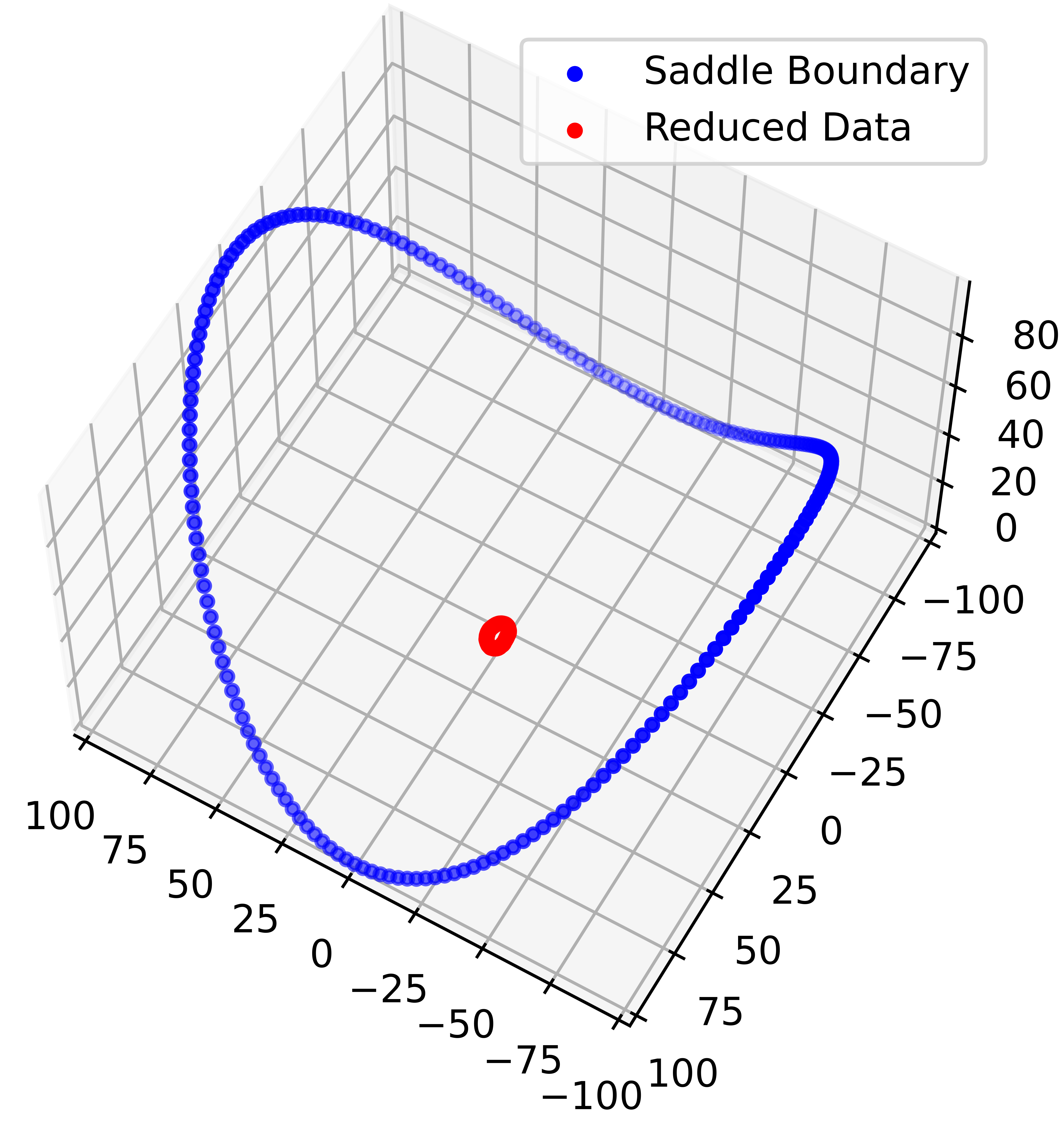
Figure 2: UMAP reduction of a saddle boundary in $\displaystyle\mathbb{R}^{3}$ to $\displaystyle\mathbb{R}^{2}$.

We can see in Figure 2 that UMAP does preserve the one-dimensional hole of the saddle boundary. However, we can also clearly see that the data has been scaled down considerably. This scaling shows up in the bottleneck distance—computing it directly, we find that $\displaystyle\operatorname{d_{B}}(X,Y)\approx 2.2$. We get the optimal scalar for the decomposition $\displaystyle\operatorname*{arg\,min}_{s}\left\lVert D_{X}-sD_{Y}\right\rVert_{\max}$ as $\displaystyle s\approx 26$. Thus it is not surprising that $\displaystyle\operatorname{d_{B}}$ performs poorly.

The normalized bottleneck performs better in this regard, with $\displaystyle\operatorname{d_{N}}(X,Y)\approx 0.012$.

4 Discussion

The normalized bottleneck $\displaystyle\operatorname{d_{N}}$ may indeed have advantages over the regular bottleneck distance when there is a large degree of scaling between two data sets. It may further have advantages over the shift-invariant bottleneck distance $\displaystyle\operatorname{d}_{\mathrm{sB}}$ [4] and the dilation-invariant bottleneck distance [2] $\displaystyle\overline{\mathrm{d}_{\rm D}}$ (see Equation 1). In practice, we do not have to compute optimal shifts/scalings in order to compute $\displaystyle\operatorname{d_{N}}$, which saves a significant amount of computational effort. Furthermore, $\displaystyle\operatorname{d_{N}}$ comes equipped as a pseudometric, allowing values for $\displaystyle\operatorname{d_{N}}$ to be compared directly.

However, in some cases the optimal scaling value may itself be useful, in which case $\displaystyle\operatorname{d_{N}}$ may not prove more useful. Furthermore, computing the optimal scaling value may indeed be necessary to obtain a tight bound from Theorem 2.10, if a bound may not already be known for $\displaystyle\left\lVert\Delta\right\rVert_{\max}$. Also, without an explicit optimal scaling value, it is unclear how much relative scaling is removed as opposed to how much scaling is being contributed from the normalization. Further work is needed to establish a relationship between $\displaystyle\operatorname{d_{N}}(X,Y)$ and $\displaystyle\displaystyle\frac{\operatorname{d_{B}}(X,Y)}{\max\{\operatorname{diam}(X),\operatorname{diam}(Y)\}}\,$.

Scaling the metric spaces by their respective diameters to define the normalized bottleneck distance (Definition 2.5) is arguably the natural choice. Alternatively, scaling by other meaningful quantities capturing the scale of the metric space, e.g., eccentricity, might yield results that are less sensitive to the largest deviation than the diameter. At the same time, deriving stability results corresponding to that for $\displaystyle\operatorname{d_{N}}$ (in Theorem 2.10) could be more challenging when the scaling is done using eccentricity.

For its application is dimension reduction, the normalized bottleneck may be examined for a broader range of techniques. Modern nonlinear reduction techniques such as UMAP [15] and t-SNE [18] may be of particular interest. In particular, while we demonstrated the effectiveness of $\displaystyle\operatorname{d_{N}}$ in practice for UMAP (see Section 3.4), it is highly desirable to derive a bound on $\displaystyle\operatorname{d_{N}}$ for UMAP similar to the one for mMDS in Corollary 3.12. Could we derive an explicit bound for $\displaystyle\left\lVert\Delta\right\rVert_{\max}$ for UMAP?

References

• [1] Shreya Arya, Jean-Daniel Boissonnat, Kunal Dutta, and Martin Lotz. Dimensionality reduction for $\displaystyle k$-distance applied to persistent homology. Journal of Applied and Computational Topology, 5:671–691, 2021. doi:10.1007/s41468-021-00079-x.
• [2] Yueqi Cao, Athanasios Vlontzos, Luca Schmidtke, Bernhard Kainz, and Anthea Monod. Topological information retrieval with dilation-invariant bottleneck comparative measures. ArXiv e-prints, 2021. https://arxiv.org/abs/2104.01672. arXiv:2104.01672.
• [3] Gunnar Carlsson. Topology and data. Bulletin of the American Mathematical Society, 46(2):255–308, January 2009. doi:10.1090/s0273-0979-09-01249-x.
• [4] Nicholas J. Cavanna, Oliver Kiselius, and Donald R. Sheehy. Computing the Shift-Invariant Bottleneck Distance for Persistence Diagrams. In Proceedings of the Canadian Conference on Computational Geometry, 2018.
• [5] Frédéric Chazal, Vin de Silva, Marc Glisse, and Steve Oudot. The Structure and Stability of Persistence Modules. SpringerBriefs in Mathematics. Springer Cham, 1 edition, 2016.
• [6] Frédéric Chazal, Vin de Silva, and Steve Oudot. Persistence stability for geometric complexes. Geometriae Dedicata, 173:193–214, 2014. doi:10.1007/s10711-013-9937-z.
• [7] Ryan G. Coleman and Kim A. Sharp. Finding and characterizing tunnels in macromolecules with application to ion channels and pores. Biophysical Journal, 96(2):632–645, 2009.
• [8] Trevor F. Cox and Michael A.A. Cox. Multidimensional Scaling. Chapman & Hall/CRC Monographs on Statistics & Applied Probability. CRC Press, 2nd edition, 2000.
• [9] Erik Demaine, Adam Hesterberg, Frederic Koehler, Jayson Lynch, and John Urschel. Multidimensional Scaling: Approximation and Complexity. In Marina Meila and Tong Zhang, editors, Proceedings of the 38th International Conference on Machine Learning, volume 139 of Proceedings of Machine Learning Research, pages 2568–2578. PMLR, 18–24 Jul 2021. URL: https://proceedings.mlr.press/v139/demaine21a.html.
• [10] Herbert Edelsbrunner and John L. Harer. Computational Topology An Introduction. American Mathematical Society, December 2009.
• [11] Herbert Edelsbrunner and Dmitriy Morozov. Persistent Homology: Theory and Practice. Lawrence Berkeley National Laboratory eScholarship, 2013. URL: https://escholarship.org/uc/item/2h33d90r.
• [12] William B. Johnson and Joram Lindenstrauss. Extensions of Lipschitz mappings into a Hilbert space, volume 26 of Contemporary Mathematics, pages 189–206. 1984.
• [13] Martin Lotz. Persistent homology for low-complexity models. Proceedings of the Royal Society A: Mathematical, Physical and Engineering Sciences, 475(2230):20190081, 2019. doi:10.1098/rspa.2019.0081.
• [14] Sepideh Mahabadi, Konstantin Makarychev, Yury Makarychev, and Ilya Razenshteyn. Nonlinear Dimension Reduction via Outer Bi-Lipschitz Extensions. In Proceedings of the 50th Annual ACM SIGACT Symposium on Theory of Computing, STOC 2018, pages 1088–1101, New York, NY, USA, 2018. Association for Computing Machinery. doi:10.1145/3188745.3188828.
• [15] Leland McInnes, John Healy, and James Melville. UMAP: Uniform Manifold Approximation and Projection for Dimension Reduction. ArXiv e-prints, September 2020. https://arxiv.org/abs/1802.03426. arXiv:1802.03426.
• [16] Donald R. Sheehy. The persistent homology of distance functions under random projection. In Proceedings of the Thirtieth Annual Symposium on Computational Geometry, SOCG’14, pages 328––334, New York, NY, USA, 2014. Association for Computing Machinery. doi:10.1145/2582112.2582126.
• [17] Joshua B. Tenenbaum, Vin de Silva, and John C. Langford. A global geometric framework for nonlinear dimensionality reduction. Science, 290(5500):2319–2323, 2000.
• [18] Laurens van der Maaten and Geoffrey Hinton. Visualizing data using t-SNE. Journal of machine learning research, 9(Nov):2579–2605, 2008.
• [19] Alexander Wagner, Elchanan Solomon, and Paul Bendich. Improving metric dimensionality reduction with distributed topology, 2021. URL: https://arxiv.org/abs/2106.07613.
• [20] Lin Yan, Yaodong Zhao, Paul Rosen, Carlos Scheidegger, and Bei Wang. Homology-preserving dimensionality reduction via manifold landmarking and tearing. In Proceedings of the Symposium on Visualization in Data Science (VDS) at IEEE VIS, volume 2018, pages 1–9, 2018.