Survival of one dimensional renewal contact process

Abstract.

The renewal contact process, introduced in $2019$ by Fontes, Marchetti, Mountford, and Vares, extends the Harris contact process in $\mathbb{Z}^{d}$ by allowing the possible cure times to be determined according to independent renewal processes (with some interarrival distribution $\mu$) and keeping the transmission times determined according to independent exponential times with a fixed rate $\lambda$. We investigate sufficient conditions on $\mu$ to have a process with a finite critical value $\lambda_{c}$ for any spatial dimension $d\geq 1$. In particular, we show that $\lambda_{c}$ is finite when $\mu$ is continuous with bounded support or when $\mu$ has a decreasing hazard rate.

Keywords: Contact process, percolation, renewal process.

1. Introduction

The classical contact process, introduced by Harris [6] in $1974$, is a model for the spread of infectious diseases and has been intensively studied (see for instance [1] and [9]). Several variants and extensions appeared in the literature, including the Renewal Contact Process, which is the model studied in this paper and was introduced in [2], [4], motivated by questions regarding long range percolation.

In both models, the sites of $\mathbb{Z}^{d}$ represent individuals that can be healthy or infected, and the state of the population at time $t$ is represented by a configuration $\xi_{t}\in\{0,1\}^{\mathbb{Z}^{d}}$, where $\xi_{t}(x)=0$ means that the individual $x$ is healthy at time $t$ and $\xi_{t}(x)=1$ means that the individual $x$ is sick at time $t$. The classical model considers a Markovian evolution: Infected individuals become healthy at rate $1$ independently of everything else, and healthy individuals become sick at a rate equal to a given parameter $\lambda$ times the number of infected neighbors. The Renewal Contact Process extends this model by allowing the possible cure times to be determined by i.i.d. renewal processes with an interarrival distribution $\mu$ on $[0,\infty)$ such that $\mu\{0\}<1$. This model will be denoted by RCP($\mu$). This additional flexibility comes with the cost of losing the Markov property, which brings new difficulties.

In [7] the classical contact process was alternatively defined using a percolation structure, known as graphical representation, in terms of a system of infinitely many independent Poisson point processes. This is a very useful tool to prove important properties of the process. It was exploited in [2, 4] adapted to the RCP($\mu$) and also in the more recent [5, 8] for more general percolation structures, replacing Poisson point processes with more general point processes. The graphical construction will be used during the proofs presented in this paper. Among the main questions of interest regarding the RCP($\mu$) we want to better understand the survival and extinction of the infection depending on the parameter $\lambda$ and the distribution $\mu$. In this direction, given $\mu$, the critical parameter for the RCP($\mu$) is defined as

$$\lambda_{c}(\mu):=\inf\{\lambda:P(\tau^{\{0\}}=\infty)>0\},$$

where $\tau^{\{0\}}:=\inf\{t:\xi_{t}^{\{0\}}\equiv 0\}$ (with the usual convention that $\inf\emptyset=\infty$) and $\xi_{t}^{\{0\}}$ denotes the RCP($\mu$) at time $t$ when started only with the origin infected at time $0$. The articles [2] and [3] (this last one for finite volumes) obtained sufficient conditions on $\mu$ to assure that $\lambda_{c}(\mu)=0$ (when $\mu$ has a heavy tail), while [4] obtained sufficient conditions on $\mu$ to assure that $\lambda_{c}(\mu)>0$, and which were significantly relaxed in [5]. In particular, the authors in [5] proved that $\lambda_{c}(\mu)>0$ whenever $\int x^{\alpha}\mu(dx)<\infty$ for some $\alpha>1$. Even combining the results of [2] and [5], there remains an important gap where we do not know whether the critical parameter is zero or not.

As we can see from the previous paragraph, the study of sufficient conditions to assure that $\lambda_{c}(\mu)$ is zero or positive is already intense. Nevertheless, it is also natural to ask whether $\lambda_{c}(\mu)$ is finite or infinite and this question was very little explored in the literature until now. Naturally if $\mu$ is degenerate (there exists $c>0$ such that $\mu\{c\}=1$), the infection always dies out (at time $c$) and consequently $\lambda_{c}(\mu)=\infty$. It is natural to conjecture that except by this degenerate case (simultaneous extinction), the critical parameter should be finite, but we still do not have a proof for that in the literature. Since $\lambda_{c}(\mu)$ is non-increasing in $d$, it is enough to consider the one-dimensional case. When $d\geq 2$, this problem becomes much simpler since we can construct an infinite infection path using each vertex only once (i.e. through a coupling with supercritical oriented percolation), avoiding dependencies within each renewal process. This idea was explored in the proof of Theorem $1.3(ii)$ in [8], which proves that the critical parameter is finite considering a more general version of the Renewal Contact Process and the proof for the RCP($\mu$) would be analogous.

Considering $d=1$, and obviously excluding the cases where we already know that $\lambda_{c}(\mu)=0$, the only general result that we have regarding $\lambda_{c}(\mu)<\infty$ is the one described in Remark $2.2$ of [5]. It argues that if $\mu$ has a density and a bounded decreasing hazard rate, then $\lambda_{c}(\mu)$ is finite. The proof uses a coupling of the RCP($\mu$) with the classical contact process using the construction described in [4]. In particular, if $\mu$ and $\tilde{\mu}$ are absolutely continuous distribution on $[0,\infty)$ with hazard rates $h_{\mu}$ and $h_{\tilde{\mu}}$ such that $h_{\mu}(t)\leq h_{\tilde{\mu}}(t)$ for any $t\geq 0$ and moreover $h_{\mu}(t)$ is decreasing in $t$ and then $\lambda_{c}(\mu)\leq\lambda_{c}(\tilde{\mu})$.

This paper focuses on proving that $\lambda_{c}(\mu)$ is finite considering the RCP($\mu$) in $d=1$ under more general conditions of $\mu$ and has two main results in this direction. The first theorem states that $\lambda_{c}(\mu)$ is finite whenever $\mu$ is continuous and has a bounded support.

Theorem 1.1.

Let $\mu$ be a continuous distribution such that $\mu[0,b]=1$ for some $b<\infty$. Then $\lambda_{c}(\mu)<\infty$.

The second theorem states that $\lambda_{c}(\mu)$ is finite whenever $\mu$ has a decreasing hazard rate. This improves over Remark $2.2$ of [5] by allowing the hazard rate to be unbounded near the origin. Our theorem covers for example the case where the times between cure marks have a Weibull distribution with the shape parameter being smaller than one.

Theorem 1.2.

Let $\mu$ be an absolutely continuous distribution on $[0,\infty)$ with density $f$ and distribution function $F$ such that its hazard rate $\frac{f(t)}{1-F(t)}$ is decreasing in $t$. Then $\lambda_{c}(\mu)<\infty$.

In Section 2 we have the proof of Theorem 1.1 and Section 3 is dedicated to the proof of Theorem 1.2. Both proofs involve coupling with supercritical oriented percolation. Differently from [8], we need to find a way to do it using the same vertices more than once to construct an infinite path, and therefore it is necessary to control the dependency problem. Each proof addressed this problem in a different manner, and we still could not find a way to deal with it for any non-degenerate $\mu$, keeping us from proving the conjecture mentioned before.

To conclude, we introduce some notation that will be used throughout the paper:

$\bullet$ $(\mathcal{R}_{x})_{x\in\mathbb{Z}}$ is a family of independent renewal processes with interarrival distribution $\mu$ and starting time $\tau\leq 0$ (possibly different for different values of $x$). $\mathcal{R}_{x}$ describes the cure marks at $x$. When the specific vertex is not important we will denote simply by $\mathcal{R}$ the renewal process constructed in the same way as these $\mathcal{R}_{x}$.

$\bullet$ $(\mathcal{N}_{(x,y)})_{(x,y)\in\mathcal{E}}$ is a family of independent Poisson processes with rate $\lambda$. Here $\mathcal{E}$ denotes the set of ordered pairs of nearest neighbors in $\mathbb{Z}$. $\mathcal{N}_{(x,y)}$ describes the times when the vertex $x$ tries to infect $y$.

2. $\mu$ continuous and with bounded support

This section is devoted to proving Theorem 1.1. Before this, we need to state and prove some useful lemmas.

The first lemma gives a control on the distance between two cure marks in adjacent vertices (we will use it for adjacent vertices, but all that matters is to have two independent renewal processes).

Lemma 2.1.

Let $\mu$ be a continuous distribution and $\mathcal{R}$, $\tilde{\mathcal{R}}$ be two independent renewal processes with interarrival distribution $\mu$. Denote by $S_{i}=S_{x,i}$ the time of the $i-th$ renewal of $\mathcal{R}$ and fix $p_{0}\in(0,1)$. Then uniformly on $\tau$, for any $i\in\mathbb{N}$, there exists $w_{0}=w_{0}(p_{0})$ such that:

$$P(\tilde{\mathcal{R}}\cap[S_{i}-w_{0},S_{i}+w_{0}]\neq\emptyset\mid S_{i})\leq p_{0}.$$

Lemma 2.1 allows us to state a corollary that gives control over how close the cure marks of two adjacent vertices inside a finite time interval are from each other.

Corollary 2.2.

Let $\mu$ be a continuous distribution and $\mathcal{R}$, $\tilde{\mathcal{R}}$ be two independent renewal processes with interarrival distribution $\mu$. For any fixed $t\geq 0$ and $s>0$, denote by $S_{j}=S_{j}(t,s)$ the $j-th$ renewal mark of the process $\mathcal{R}$ inside the time interval $[t,t+s]$ and by $N=N(t,s)$ the number of renewal marks of $\mathcal{R}$ inside this time interval. Also define $\tilde{S}_{j}$ and $\tilde{N}$ in the same way of $S_{j}$ and $N$ but considering $\tilde{\mathcal{R}}$ instead of $\mathcal{R}$. Fix $K_{1}\in\mathbb{N}$ and $K_{2}\in\mathbb{N}$ such that $P(N\leq K_{1})>0$ and $P(\tilde{N}\leq K_{2})>0$. Then, for any fixed $p_{0}\in(0,1)$, $s>0$, $K_{1}$, $K_{2}$ and $\omega_{0}\in(0,s)$, there exists $v_{0}=v_{0}(p_{0},s,K_{1},K_{2},\omega_{0})>0$ such that:

$$\sup_{t\geq 0}P\Big{(}\min_{1\leq i\leq N}\min_{1\leq j\leq\tilde{N}}\Big{|}\tilde{S}_{j}-S_{i}\Big{|}\leq v_{0}\ \Big{|}N\leq K_{1},\tilde{N}\leq K_{2},S_{1}\geq t+\omega_{0}\Big{)}\leq p_{0}.$$

The next lemma gives us control over the number of renewal marks that appear on a vertex during a finite period of time.

Lemma 2.3.

Let $\mathcal{R}$ be a renewal process with interarrival distribution $\mu$ continuous. Fix $p_{0}\in(0,1)$ and $b>0$. Then uniformly on $\tau$, there exists $K_{0}=K_{0}(p_{0},b)$ such that:

$$\sup_{t\geq 0}P(\ |\ \mathcal{R}\cap[t,t+3b]\ |>K_{0})\leq p_{0}.$$

Now the next two lemmas state that if we choose $\lambda$ large enough, the infection can survive inside specific space-time boxes with high probability. For both lemmas, consider the RCP($\mu$) where $\mu$ is a continuous distribution such that $\mu[0,b]=1$.

Lemma 2.4.

Fix $b>0$, let $B_{h}(x,t)=[x,x+3]\times[t,t+b]$ be a space-time box that we will call “horizontal box” and fix $\epsilon\in(0,1)$. Assuming that the vertex $x$ or $x+1$ is infected at time $t$, denote by $C_{h}(x,t)$ the event $\{$the infection reaches the vertex $x+3$ inside $B_{h}(x,t)\}$ and when it happens, we will say that we have a horizontal crossing of the box $B_{h}(x,t)$. Then uniformly on $\tau$ and for any $x$, there exists $\lambda_{h}=\lambda_{h}(\epsilon)<\infty$ such that:

$$\inf_{t\geq 0}P(C_{h}(x,t))\geq 1-\epsilon,\ \mbox{if}\ \lambda>\lambda_{h}.$$

Lemma 2.5.

Fix $b>0$, let $B_{v}(x,t)=[x,x+1]\times[t,t+3b]$ be a space-time box that we will call “vertical box” and fix $\epsilon\in(0,1)$. Assuming that the vertex $x$ or $x+1$ is infected at time $t$, denote by $C_{v}(x,t)$ the event $\{$the infection survives up to time $t+3b$ inside $B_{v}(x,t)\}$ and when it happens we will say that we have a vertical crossing of the box $B_{v}(x,t)$. Then uniformly on $\tau$ and for any $x$, there exists $\lambda_{v}=\lambda_{v}(\epsilon)<\infty$ such that:

$$\inf_{t\geq 0}P(C_{v}(x,t))\geq 1-\epsilon,\ \mbox{if}\ \lambda>\lambda_{v}.$$

Proof.

(Lemma 2.1) Since the renewal processes $\mathcal{R}$ and $\tilde{\mathcal{R}}$ are independent, we have that:

$$P(\tilde{\mathcal{R}}\cap[S_{i}-w_{0},S_{i}+w_{0}]\neq\emptyset\mid S_{i})\leq\sup_{t\geq 0}P(\tilde{\mathcal{R}}\cap[t-w_{0},t+w_{0}]\neq\emptyset).$$

From now on the proof follows the same arguments presented in the proof of Lemma 4.1(ii) in [8]. ∎

Proof.

(Corollary 2.2) Assume that $N=n_{1}\leq K_{1}$. Now for any finite collection of points $\underline{u}=\{u_{1},u_{2},\ldots u_{n_{1}}\}$ inside $[t+\omega_{0},t+s]$ and any $v>0$, denote $\mathcal{C}_{\underline{u}}(v)=\bigcup_{i=1}^{n_{1}}[u_{i}-v,u_{i}+v]$. We have that

$$P\Big{(}\bigcup_{j=1}^{\tilde{N}}\{\tilde{S}_{j}\in\mathcal{C}_{\underline{u}}(v)\}\Big{|}\tilde{N}\leq K_{2}\Big{)} =\sum_{n_{2}=1}^{K_{2}}P\Big{(}\bigcup_{j=1}^{n_{2}}\{\tilde{S}_{j}\in\mathcal{C}_{\underline{u}}(v)\}\Big{|}\tilde{N}=n_{2}\Big{)}P(\tilde{N}=n_{2}\mid\tilde{N}\leq K_{2})$$

$$\leq K_{2}\max_{1\leq n_{2}\leq K_{2}}\Big{[}P\Big{(}\bigcup_{j=1}^{n_{2}}\{\tilde{S}_{j}\in\mathcal{C}_{\underline{u}}(v)\}\Big{|}\tilde{N}=n_{2}\Big{)}P(\tilde{N}=n_{2}\mid\tilde{N}\leq K_{2})\Big{]}$$

$$\leq K_{2}\max_{1\leq n_{2}\leq K_{2}}\sum_{j=1}^{n_{2}}P(\tilde{S}_{j}\in\mathcal{C}_{\underline{u}}(v)\mid\tilde{N}\leq K_{2})$$

$$\qquad\qquad\ \ \leq\frac{K_{2}^{2}}{P(\tilde{N}\leq K_{2})}\max_{1\leq n_{2}\leq K_{2}}\max_{1\leq j\leq n_{2}}P(\tilde{S}_{j}\in\mathcal{C}_{\underline{u}}(v)).$$ (2.1)

Now, by Lemma 2.1, for any fixed $p_{0}\in(0,1)$ and $t\geq 0$ and $j=1,2,\ldots n_{2}$, we can choose $v=v(p_{0},s,K_{1},K_{2},w_{0},\underline{u})>0$ such that the probability in (2.1) is smaller than $\frac{P(\tilde{N}\leq K_{2})}{K_{2}^{2}}p_{0}$ for any $t\geq 0$.

Since the previous arguments hold for any possible choice of the points $\underline{u}=$ $\{u_{1},u_{2},\ldots u_{n_{1}}\}$ inside $[t+\omega_{0},t+s]$, we can take $v_{0}=v_{0}(p_{0},s,K_{1},K_{2},w_{0})>0$ such that the probability on (2.1) become smaller than $\frac{P(\tilde{N}\leq K_{2})}{K_{2}^{2}}p_{0}$ for every possible choice of $\underline{u}$. Since $\mathcal{R}$ and $\tilde{\mathcal{R}}$ are independent renewal processes, we can just observe the realization of $N$ (denote by $n_{1}$ this result) and $(S_{i})_{1\leq i\leq n_{1}}$. After that, we can take $u_{i}$ equal to the realization of $S_{i}$ and then,

$$\sup_{t\geq 0}P\Big{(}\min_{1\leq i\leq N}\min_{1\leq j\leq\tilde{N}}\Big{|}\tilde{S}_{j}-S_{i}\Big{|}\leq v_{0}\ \Big{|}N\leq K_{1},\tilde{N}\leq K_{2},S_{1}\geq t+\omega_{0}\Big{)}$$

$$\leq P\Big{(}\bigcup_{j=1}^{\tilde{N}}\{\tilde{S}_{j}\in\mathcal{C}_{\underline{u}}(v_{0})\}\Big{|}\tilde{N}\leq K_{2}\Big{)}\leq p_{0}.\qquad\qquad\qquad\qquad\qquad\qquad\vspace{-0.6cm}$$

∎

Proof.

(Lemma 2.3) First note that we can remove the supreme if we assume the existence of a renewal mark at time $t=0$ and want to have at least $K_{0}$ renewals in the interval $(t,t+3b]$. Denoting by $(X_{j})_{j\geq 1}$ a sequence of i.i.d random variables with distribution $\mu$, we can write:

$$\sup_{t\geq 0}P(\ |\ \mathcal{R}\cap[t,t+3b]\ |>K)\leq P\Big{(}\sum_{j=1}^{K-1}X_{j}<3b\Big{)}=P\Big{(}\frac{1}{K-1}\sum_{j=1}^{K-1}X_{j}<\frac{3b}{K-1}\Big{)}.$$ (2.2)

If $K\to\infty$, we have that $\frac{1}{K-1}\sum_{j=1}^{K-1}X_{j}$ converges to $E[X_{1}]>0$ by the law of large numbers and $\frac{3b}{K-1}$ converges to zero. So, for any fixed $p_{0}>0$ and $b>0$, we can choose $K_{0}$ large enough such that the rightmost probability in (2.2) becomes smaller than $p_{0}$. ∎

Proof.

(Lemma 2.4) By hypothesis of the Lemma, the vertex $x$ or $x+1$ is infected at time $t$, so let’s assume without loss of generality that vertex $x$ is infected at time $t$. Denote by $E_{0}^{(t)}$ the event $\{$the vertex $x$ transmits the infection to the vertex $x+1$ before time $t+0,3b$ and before it reaches a cure mark$\}$. Similarly, denote $E_{i}^{(s_{i})}$, for $i=1,2$ the event $\{$ after the vertex $x+i$ gets infected (let’s denote by $s_{i}$ the time that it happened), it transmits the infection to the vertex $x+i+1$ before time $s_{i}+0.3b$ and before it reaches a cure mark$\}$. To simplify the notation, let $s_{0}=t$. We have that

$$\inf_{t\geq 0}P(C_{h}(x,t))\geq\inf_{s_{0}\geq 0}\inf_{s_{1}\geq 0}\inf_{s_{2}\geq 0}P\Big{(}E_{0}^{(s_{0})}\cap E_{1}^{(s_{1})}\cap E_{2}^{(s_{2})}\Big{)}\qquad\qquad\qquad$$

$$\qquad\qquad\qquad\qquad\geq\inf_{s_{0}\geq 0}P\Big{(}E_{0}^{(s_{0})}\Big{)}\inf_{s_{1}\geq 0}P\Big{(}E_{1}^{(s_{1})}\Big{|}E_{0}^{(s_{0})}\Big{)}\inf_{s_{2}\geq 0}P\Big{(}E_{2}^{(s_{2})}\Big{|}E_{1}^{(s_{1})}\Big{)}.$$

Now we will create two collections of events $F_{i}^{(s_{i})}$ and $G_{i}^{(s_{i})}$, for $i=0,1,2$, such that when they occur together, the event $E_{i}^{(s_{i})}$ also occurs. Let $F_{i}^{(s_{i})}(a)$ be the event $\{\mathcal{R}_{x+i}\cap[s_{i},s_{i}+a]=\emptyset\}$, and $G_{i}^{(s_{i})}(a)$ be the event $\{$the vertex $x+i$ transmit the infection to vertex $x+i+1$ in the time interval $[s_{i},s_{i}+a]\}$. In Figure 1 we have an illustration of the event $C_{h}(t,x)$ occurring. Note that, for any fixed $0<a<0,3b$;

$$\inf_{s_{0}\geq 0}P\Big{(}E_{0}^{(s_{0})}\Big{)}\geq\inf_{s_{0}\geq 0}P\Big{(}G_{0}^{(s_{0})}(a)\Big{|}F_{0}^{(s_{0})}(a)\Big{)}P\Big{(}F_{0}^{(s_{0})}(a)\Big{)}\qquad\ \$$

$$\qquad\qquad=P\Big{(}G_{0}^{(s_{0})}(a)\Big{|}F_{0}^{(s_{0})}(a)\Big{)}\inf_{s_{0}\geq 0}P\Big{(}F_{0}^{(s_{0})}(a)\Big{)},$$ (2.3)

where the equality in (2.3) appears because the probability of the event $G_{0}^{(s_{0})}(a)$ given $F_{0}^{(s_{0})}(a)$ depends only on the probability of having a transmission attempt during a time interval of length $a$, which does not depend on the specific position of the interval $[s_{i},s_{i}+a]$. The same kind of lower bound that is present in (2.3) works for $\inf_{s_{i}\geq 0}P(E_{i}^{(s_{i})}|E_{i-1}^{(s_{i-1})})$, replacing $G_{0}^{(s_{0})}(a)$ and $F_{0}^{(s_{0})}(a)$ by $G_{i}^{(s_{i})}(a)$ and $F_{i}^{(s_{i})}(a)$.

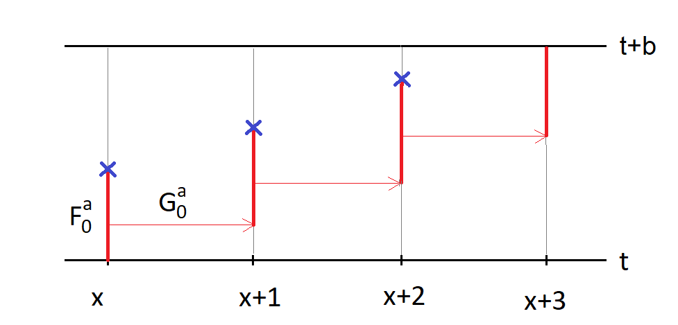
Figure 1. Illustration of a horizontal crossing inside the box $B_{h}(t,x)$. The red lines indicate the infection path, the red arrows indicate the transmissions and the X marks indicate the cures. $F_{0}^{a}=F_{0}^{(t)}(a)$ and $G_{0}^{a}=G_{0}^{(t)}(a)$.

To begin the control of the probabilities in (2.3), let’s fix $p_{0}=1-(1-\epsilon)^{\frac{1}{6}}$. By Lemma 4.1(ii) of [8], there exists $w_{0}=w_{0}(p_{0})>0$ such that $\inf_{s_{i}\geq 0}P(F_{i}^{(s_{i})}(w_{0}))\geq 1-p_{0}$ for any $i=0,1,2$. If we take $a_{0}=\min(w_{0};0,3)$, we also have

$$\inf_{s_{i}\geq 0}P\Big{(}F_{i}^{(s_{i})}(a_{0})\Big{)}\geq 1-p_{0}=(1-\epsilon)^{\frac{1}{6}}.$$

Since $a_{0}>0$, we can fix $\lambda_{h}$ such that $P(\exp(\lambda_{h})\leq a_{0})=(1-\epsilon)^{\frac{1}{6}}$, which is equivalently to fix $\lambda_{h}=\frac{-1}{a_{0}}\log(1-[1-\epsilon]^{\frac{1}{6}})$. With this value of $\lambda_{h}$ we have

$$P\Big{(}G_{i}^{(s_{i})}(a_{0})\Big{|}F_{i}^{(s_{i})}(a_{0})\Big{)}=(1-\epsilon)^{\frac{1}{6}},$$

and consequently:

$$\inf_{t\geq 0}P(C_{h}(x,t))\geq\prod_{i=0}^{2}\Big{[}P\Big{(}G_{i}^{(s_{i})}(a_{0})\Big{|}F_{i}^{(s_{i})}(a_{0})\Big{)}\inf_{s_{i}\geq 0}P\Big{(}F_{i}^{(s_{i})}(a_{0})\Big{)}\Big{]}\geq\Big{[}(1-\epsilon)^{\frac{1}{6}}(1-\epsilon)^{\frac{1}{6}}\Big{]}^{3}=1-\epsilon.\vspace{-0.2cm}$$

∎

Proof.

(Lemma 2.5) Suppose without loss of generality that only the vertex $x$ is infected at time $t$.

Note that since the box $B_{v}(x,t)$ has only two vertices, the infection has to keep jumping between these two vertices until time $t+3b$. In Figure 2 we have an illustration of event $C_{v}(x,t)$ occurring.

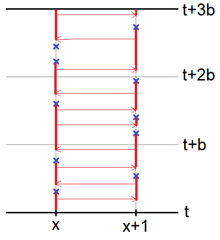
Figure 2. Illustration of a vertical crossing inside the box $B_{v}(x,t)$. The red lines indicate the infection path, the red arrows indicate the transmissions and the X marks indicate the cures.

So, our strategy will be the following: First, we will look to the cure marks of vertices $x$ and $x+1$ inside the box $B_{v}(x,t)$ and say that these marks are “good” if they satisfy an event $A_{t}$ that will be explained later. Then we can write:

$$\inf_{t\geq 1}P(C_{v}(x,t))=\inf_{t\geq 1}\Big{[}P(C_{v}(x,t)|A_{t})P(A_{t})+P(C_{v}(x,t)|A_{t}^{c})P(A_{t}^{c})\Big{]}\geq\inf_{t\geq 1}P(C_{v}(x,t)|A_{t})P(A_{t}).$$

After that, we will say that the attempts of transmissions inside the box $B_{v}(x,t)$ are “good” if they satisfy an event $V$ that will be explained later. This event $V$ will be chosen such that the occurrence of $A_{t}$ and $V$ together guarantees the occurrence of $C_{v}(x,t)$. An important detail here is that since the cure marks are independent of the transmission attempts, then the event $A_{t}$ will depend only on the distribution of the cure times, and the event $V$ given $A_{t}$ will depend only on the distribution of infection times.

To begin let $N$ and $\tilde{N}$ be the number of cure marks of vertex $x$ and $x+1$ inside the time interval $[t,t+3b]$ respectively. Also let $S_{i}$ and $\tilde{S}_{i}$ be the time of the $i-th$ cure mark of vertex $x$ and $x+1$ inside the box $B_{v}(x,t)$ respectively. Now fix $p_{0}=1-(1-\epsilon)^{\frac{1}{8}}$. By Lemma 2.3, there exists $K_{0}$ such that $P(N\leq K_{0})\geq 1-p_{0}=(1-\epsilon)^{\frac{1}{8}}$. It is also true if we assume that $S_{1}\geq t+w$ for any $w>0$, since in this case we already know that we do not have any renewal mark inside the interval $[t,t+w]$ and it just turns easier to have at most $K_{0}$ renewal marks in $[t,t+3b]$. Then, since the cure marks of different vertices are independent, we also have for any fixed $w>0$ and for any $t\geq 0$:

$$P(N\leq K_{0},\tilde{N}\leq K_{0}\mid S_{1}\geq t+w)\geq(1-\epsilon)^{\frac{1}{4}}.$$ (2.4)

Now fix $p_{1}=1-(1-\epsilon)^{\frac{1}{8}}$. By Lemma 4.1(ii) of [8] there exists $w_{1}=w_{1}(p_{1})$ such that:

$$\inf_{t\geq 0}P(S_{1}\geq t+w_{1})\geq 1-p_{1}=(1-\epsilon)^{\frac{1}{8}}.$$ (2.5)

From now on fix $w_{1}$ as the biggest value that satisfies (2.5) and fix $K_{0}$ as the smallest integer value that satisfies (2.4) with $w=w_{1}$. Note that if we condition on the occurrence of the event $\{N\leq K_{0},\tilde{N}\leq K_{0}\}$, then we have at most $K_{0}$ random variables $S_{i}$ and $\tilde{S}_{i}$. Hence, by Corollary 2.2 there exists $v_{1}=v_{1}(p_{1})$ such that for any $t\geq 0$:

$$P\Big{(}\min_{1\leq i\leq K_{0}}\min_{1\leq j\leq K_{0}}\left|\tilde{S}_{j}-S_{i}\right|\geq v_{1}\Big{|}N\leq K_{0},\tilde{N}\leq K_{0},S_{1}\geq t+w_{1}\Big{)}\geq 1-p_{1}=(1-\epsilon)^{\frac{1}{8}}.$$ (2.6)

From now on, fix $v_{1}$ as the biggest value that satisfies (2.6). At this point, we will define the event $A_{t}$, which identifies if the cure marks are “good” or not. Let $A_{t}=A^{(t)}_{1}\cap A^{(t)}_{2}\cap A^{(t)}_{3}$ where:

$$A_{1}^{(t)}=\Big{\{}\min_{1\leq i\leq K_{0}}\min_{1\leq j\leq K_{0}}\left|\tilde{S}_{j}-S_{i}\right|\geq v_{1}\Big{\}},\ \ A_{2}^{(t)}=\left\{N\leq K_{0},\tilde{N}\leq K_{0}\right\},\ \ A_{3}^{(t)}=\Big{\{}S_{1}\geq t+w_{1}\Big{\}}.$$

Then, by (2.4), (2.5) and (2.6) we have that

$$\inf_{t\geq 1}P(A_{t})=\inf_{t\geq 1}P\Big{(}A_{1}^{(t)}\Big{|}A_{2}^{(t)}\cap A_{3}^{(t)}\Big{)}P\Big{(}A_{2}^{(t)}\Big{|}A_{3}^{(t)}\Big{)}P\Big{(}A_{3}^{(t)}\Big{)}\geq(1-\epsilon)^{\frac{1}{8}}(1-\epsilon)^{\frac{1}{4}}(1-\epsilon)^{\frac{1}{8}}=(1-\epsilon)^{\frac{1}{2}}.$$

Now define a sequence of $M+2$ increasing times $(\tau_{i})_{i\geq 0}$ inside $[t,t+3b]$ in the following way: $\tau_{0}=t$, $\tau_{1}=S_{1}$, $\tau_{i}=\min\{\mathcal{R}_{x+1}\cap(\tau_{i-1},\infty)\}$ for $i\leq M$ even, $\tau_{i}=\min\{\mathcal{R}_{x}\cap(\tau_{i-1},\infty)\}$ for $1<i\leq M$ odd and $\tau_{M+1}=t+3b$.

Recall that $(\mathcal{N}_{x,y})_{(x,y)\in\mathcal{E}}$ denote the Poisson processes that describe the times when the vertex $x$ tries to infect $y$. Then, we can define $(H_{i}^{(t)})_{i\geq 1}$ the event $\{$ the infection reaches time $\tau_{i}$ inside the box $B_{v}(x,t)$ given that it reached time $\tau_{i-1}\}$. Note that $P(H_{1}^{(t)})=P(H_{M+1}^{(t)})=1$ for any $t\geq 0$. Besides that, since $\mathcal{N}_{x,y}$ has the same distribution of $\mathcal{N}_{y,x}$, then for $2\leq i\leq M$,

$$P\Big{(}H_{i}^{(t)}\Big{)}=P(\mathcal{N}_{x,x+1}\cap(\tau_{i-1},\tau_{i}]\neq\emptyset).$$

Denote by $u_{1}=w_{1}\wedge v_{1}$. Given the occurrence of $A_{t}$, we have $|\tau_{i}-\tau_{i-1}|\geq u_{1}$ for every $i=1,\ldots,M$ and the sequence $(H_{i}^{(t)})_{i\geq 1}$ will have at most $2K_{0}+1$ events. If all these events occur, then we guarantee that $C_{v}(x,t)$ occurs. Recalling that the transmissions times are given by Poisson processes with parameter $\lambda$ and denoting by $(Y_{i})_{i\geq 1}$ a sequence of i.i.d random variables with distribution $\exp(\lambda)$, we have that for any $i=2\ldots,M$:

$$\inf_{t\geq 0}P\Big{(}H_{i}^{(t)}\Big{|}A_{t}\Big{)}\geq P(Y_{i}\leq u_{1})=1-e^{-\lambda u_{1}}.$$

Now define $V$ the event $\{\max_{2\leq i\leq 2K_{0}}Y_{i}\leq u_{1}\}$. Since we have the Markov property on the transmissions,

$$\inf_{t\geq 0}P(C_{v}(x,t)|A_{t})\geq\inf_{t\geq 0}P\Big{(}\bigcap_{i=1}^{M+1}H_{i}^{(t)}\Big{|}A_{t}\Big{)}=\inf_{t\geq 0}\prod_{i=1}^{M+1}P\Big{(}H_{i}^{(t)}|A_{t}\Big{)}\geq P\Big{(}H_{1}^{(0)}\Big{)}P(V)P\Big{(}H_{M+1}^{(0)}\Big{)}$$

$$\geq(1-e^{-\lambda u_{1}})^{2K_{0}-1}.\qquad\qquad\qquad\qquad\qquad\qquad\qquad\ \ \ \$$

So, taking $\lambda_{v}=\frac{-1}{u_{1}}\log\left(1-[1-\epsilon]^{\frac{1}{4K_{0}-2}}\right)$, we have that $\inf_{t\geq 0}P(C_{v}(x,t)|A_{t})\geq(1-\epsilon)^{\frac{1}{2}}$ and hence,

$$\inf_{t\geq 0}P(C_{v}(x,t))\geq\inf_{t\geq 0}P(C_{v}(x,t)|A_{t})P(A_{t})\geq(1-\epsilon)^{\frac{1}{2}}(1-\epsilon)^{\frac{1}{2}}=1-\epsilon.$$

Then, for any $\lambda>\lambda_{v}$ we have $\inf_{t\geq 0}P(C_{v}(x,t))\geq 1-\epsilon$. ∎

Now we are finally ready to prove Theorem 1.1.

Proof.

(Theorem 1.1) Consider a graph $G$ in $\mathbb{Z}^{2}_{0\leq x\leq y+1}$ with oriented edges $z+(1,0)$ and $z+(0,1)$. Define a bond percolation in $G$ by stating that a horizontal edge from $(x,y)$ to $(x+1,y)$ is open if we have a horizontal crossing (as defined in Lemma 2.4) in the box $[2x,2x+3]\times[2yb,2yb+1]$ and that a vertical edge from $(x,y)$ to $(x,y+1)$ is open if we have a vertical crossing (as defined in Lemma 2.5) in the box $[2x,2x+1]\times[2yb,2yb+3b]$. Note that if we take $\lambda_{0}=\max(\lambda_{h},\lambda_{v})$, then the probability of an edge of $G$ being open is at least $1-\epsilon$. In Figure 3 we have the illustration of an example of this bond percolation being constructed according to the crossings in these specific boxes.

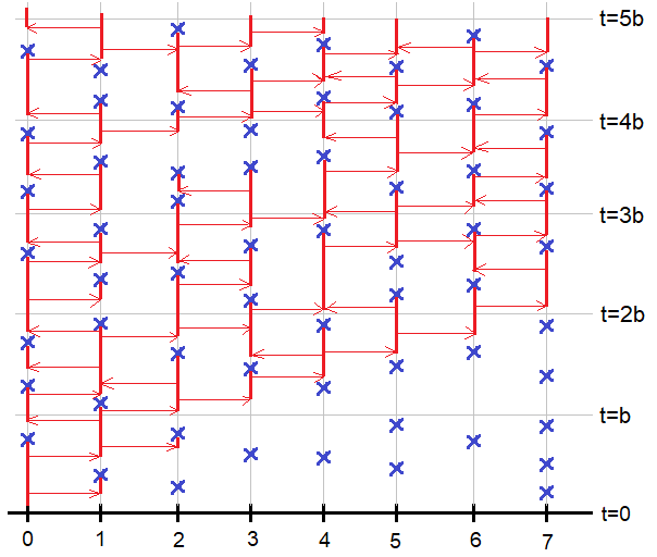
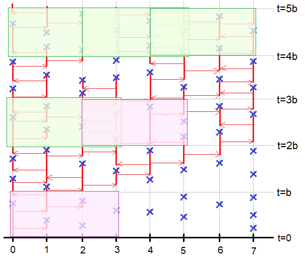
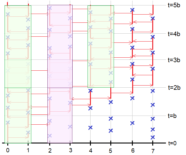
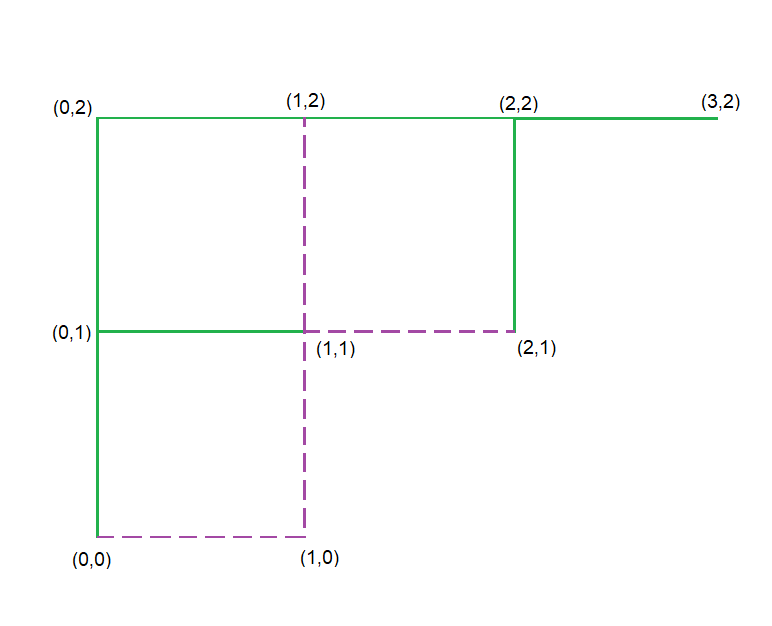
Figure 3. Example of the relation between the RCP($\mu$) and the bond percolation on G (images 1 and 4). The green boxes indicate the ones that are crossed horizontally (image 2) or vertically (image 3). The purple boxes indicate the ones that are not crossed horizontally (image 2) or vertically (image 3). In image 4 we have the open edges in green and the closed edges in dashed purple.

Now we will argue that in this bond percolation model, the edges that do not share extremities are independent. It is a consequence of three facts:

• Both transmissions and cures in different vertices are independent.

• We have Markov property for the transmissions.

• The time between two consecutive cure marks in a vertex is bounded by $b$, which means that any time interval of length $b$ will have at least one cure mark in every vertex. It implies that the cure marks after time $t+b$ are independent of the cure marks before time $t$, for any $t\geq 0$.

It means that we have a finite range dependent bond model. By the classical stochastic domination result of Liggett, Schonmann and Stacey [10], if we choose $\epsilon>0$ small enough in the beginning, it follows that the RCP with cure times given by a continuous and bounded distribution survives with positive probability if $\lambda>\lambda_{0}$. ∎

3. $\mu$ with decreasing hazard rate

This section is devoted to proving Theorem 1.2. Again, we start by stating and proving some useful lemmas.

The first and second lemmas guarantee that for any history of $\mathcal{R}_{x}$ previous to time $t$, we can find an interval (uniformly on the history of $\mathcal{R}_{x}$) that will not have any mark of the renewal process with a high fixed probability.

Lemma 3.1.

Consider $\mu$ defined in Theorem 1.2. Then, for any $\epsilon>0$, there exists $w_{0}=w_{0}(\epsilon)$ such that uniformly on $\tau$ we have

$$\sup_{t\geq 0}\sup_{k\geq 0}P\left(\left.\mathcal{R}\cap[t+k,t+k+w_{0}]\neq\emptyset\ \right|\ \mathcal{R}\cap[t,t+k]=\emptyset\right)\leq\epsilon.$$

Proof.

(Lemma 3.1) Let $(X_{j})_{j\geq 0}$ be a sequence of i.i.d. random variables with distribution $\mu$, common density $f$ and common distribution function $F$, such that $X_{0}$ describes the time until the first renewal mark of $\mathcal{R}$ and $X_{j}$, for $j\geq 1$, describe the time between the j-th and (j+1)-th renewal marks of $\mathcal{R}$. In addition, denote by $(F^{(j)})_{j\geq 0}$ the distribution function of $X_{0}+X_{1}+\ldots+X_{j}$, by $B_{t}$ the residual life process of $\mathcal{R}$ at time $t$ and by $A_{j}$ the event $\{$there are exactly $j$ renewal marks of $\mathcal{R}$ up to time $t\}$. Then, for any $t\geq 0$, $k>0$ and $w>0$, we have that

$$P\left(\left.\mathcal{R}\cap[t+k,t+k+w]\neq\emptyset\ \right|\ \mathcal{R}\cap[t,t+k]=\emptyset\right)=\sum_{j=0}^{\infty}P(B_{t}\leq k+w|B_{t}>k,A_{j}).P(A_{j})$$

$$=P(A_{0})P(X_{0}\leq t+k+w|X_{0}>t+k)+\sum_{j=1}^{\infty}P(A_{j})\int_{0}^{t}P(B_{t-s}\leq k+w|B_{t-s}>k)dF^{(j-1)}(s)\ \$$

$$=P(A_{0})\frac{P(X\in[t+k,t+k+w])}{P(X\geq t+k)}+\sum_{j=1}^{\infty}P(A_{j})\int_{0}^{t}P(X_{j}\leq t+k+w-s|X_{j}>t+k-s)dF^{(j-1)}(s)$$

$$=P(A_{0})\int_{t+k}^{t+k+w}\frac{f(u)}{1-F(t+k)}du+\sum_{j=1}^{\infty}P(A_{j})\int_{0}^{t}\left[\int_{t+k-s}^{t+k+w-s}\frac{f(u)}{1-F(t+k-s)}du\right]dF^{(j-1)}(s)\ \ \$$

$$\leq P(A_{0})\int_{t+k}^{t+k+w}\frac{f(u)}{1-F(u)}du+\sum_{j=1}^{\infty}P(A_{j})\int_{0}^{t}\left[\int_{t+k-s}^{t+k+w-s}\frac{f(u)}{1-F(u)}du\right]dF^{(j-1)}(s).\ \ \$$ (3.1)

Since the hazard rate of $\mu$ is decreasing in $t$, we have that both integrals of $\frac{f(u)}{1-F(u)}$ in (3.1) are smaller than or equal to

$$\int_{0}^{w}\frac{f(u)}{1-F(u)}du,$$

and then we easily see that (3.1) is bounded from above by

$$\frac{1}{1-F(w)}\int_{0}^{w}f(u)du\left[P(A_{0})+\sum_{j=1}^{\infty}P(A_{j})\int_{0}^{\infty}dF^{(j-1)}(s)\right]$$

$$=\frac{F(w)}{1-F(w)}\sum_{j=0}^{\infty}P(A_{j})=\frac{F(w)}{1-F(w)}.\qquad\qquad\qquad\qquad\qquad\qquad$$

Since $F$ is a continuous distribution function on $[0,\infty)$, we can take $w_{0}=w_{0}(\epsilon)>0$ such that $F(w_{0})\leq\frac{\epsilon}{2}$ and then:

$$\sup_{t\geq 0}\sup_{k\geq 0}P\left(\left.\mathcal{R}\cap[t+k,t+k+w_{0}]\neq\emptyset\ \right|\ \mathcal{R}\cap[t,t+k]=\emptyset\right)\leq\frac{F(w_{0})}{1-F(w_{0})}\leq\frac{\epsilon}{2-\epsilon}\leq\epsilon.\vspace{-0.4cm}$$

∎

Lemma 3.2.

Consider $\mu$ defined in Theorem 1.2. For any $t\geq 0$ denote by $Z_{t}$ the random variable that indicates the time of the last renewal mark of $\mathcal{R}$ previous to time $t$ (assume $Z_{t}=\tau$ if until time $t$ we do not have any renewal mark of $\mathcal{R}$). Then, for any $\epsilon>0$, there exists $w_{0}=w_{0}(\epsilon)>0$ such that uniformly on $\tau$ we have

$$\sup_{t\geq 0}\sup_{\tau\leq z\leq t}P\left(\left.\mathcal{R}\cap[t,t+w_{0}]\neq\emptyset\ \right|\ Z_{t}=z\right)\leq\epsilon.$$

Proof.

(Lemma 3.2) Let $v=t-z$. The statement is equivalent to the existence of $w_{0}=w_{0}(\epsilon)$ such that, uniformly on $\tau$, we have

$$\sup_{v\geq 0}\frac{\mu([v,v+w_{0}])}{\mu([v,\infty])}\leq\epsilon.$$

But for any fixed $w>0$ and $v>0$,

$$\frac{\mu([v,v+w])}{\mu([v,\infty])}=\int_{v}^{v+w}\frac{f(u)}{1-F(v)}du\leq\int_{v}^{v+w}\frac{f(u)}{1-F(u)}du.$$

Since the hazard rate of $\mu$ is decreasing, the last integral above is bounded by

$$\int_{0}^{w}\frac{f(u)}{1-F(u)}du\leq\frac{1}{1-F(w)}\int_{0}^{w}f(u)du=\frac{F(w)}{1-F(w)},$$

and the conclusion follows as in the previous lemma. ∎

Now Lemmas 3.1 and 3.2 together allow us to state a lemma that gives control over how close the cure marks of two adjacent vertices inside a finite time interval are from each other, uniformly on the history of the cure marks in these vertices. From now on, for any event $A$, $\overline{\mathbb{P}}_{t}^{\mu}(A)$ will denote the supremum over the probabilities of event $A$. The supremum is taken over all product renewal probability measures with interarrival distribution $\mu$ considered only up to time $t$, for the renewal marks starting at time points strictly less than $0$ (possibly different). It means that $\overline{\mathbb{P}}_{t}^{\mu}(A)=\sup P(A|\mathcal{F}_{t})$, where $\mathcal{F}_{t}$ represents the filtration generated by the renewal processes $(\mathcal{R}_{x})_{x\in\mathbb{Z}}$ up to time $t$.

Lemma 3.3.

For any fixed $x\in\mathbb{Z}$, $t\geq 0$ and $s>0$, denote by $S_{j}=S_{j}(x,t,s)$ the $j-th$ renewal mark of the process $\mathcal{R}_{x}$ inside the time interval $[t,t+s]$ and by $N=N(x,t,s)$ the number of renewal marks of the process $\mathcal{R}$ inside this time interval. Also define $\tilde{S}_{j}$ and $\tilde{N}$ in the same way of $S_{j}$ and $N$ but considering $\mathcal{R}_{x+1}$ instead of $\mathcal{R}_{x}$. For any fixed $p_{0}\in(0,1)$, $s>0$ and $w_{0}>0$, there exists $v_{0}=v_{0}(p_{0},w_{0},s)>0$ such that:

$$\sup_{t\geq 0}\overline{\mathbb{P}}_{t}^{\mu}\Big{(}\min_{1\leq i\leq N}\min_{1\leq j\leq\tilde{N}}\left|\tilde{S}_{j}-S_{i}\right|\leq v_{0}\Big{|}S_{1}\geq t+w_{0}\Big{)}\leq p_{0}.$$ (3.2)

Proof.

(Lemma 3.3) For any fixed $t\geq 0$, $s>0$, $K_{1}\in\mathbb{N}$ and $K_{2}\in\mathbb{N}$, define the following event:

$$A=A(t,s,K_{1},K_{2})=\left\{N\leq K_{1},\tilde{N}\leq K_{2}\right\}.$$

Then, we have that

$$\overline{\mathbb{P}}_{t}^{\mu}\Big{(}\min_{1\leq i\leq N}\min_{1\leq j\leq\tilde{N}}\left|\tilde{S}_{j}-S_{i}\right|\leq v\Big{|}S_{1}\geq t+w_{0}\Big{)}\qquad\qquad\qquad\qquad\qquad\qquad$$

$$\leq\overline{\mathbb{P}}_{t}^{\mu}\Big{(}\min_{1\leq i\leq N}\min_{1\leq j\leq\tilde{N}}\left|\tilde{S}_{j}-S_{i}\right|\leq v\ \Big{|}S_{1}\geq t+w_{0},A\Big{)}\overline{\mathbb{P}}_{t}^{\mu}(\left.A\right|S_{1}\geq t+w_{0})\qquad\ \ \$$

$$+\hskip 2.27626pt\overline{\mathbb{P}}_{t}^{\mu}\Big{(}\min_{1\leq i\leq N}\min_{1\leq j\leq\tilde{N}}\left|\tilde{S}_{j}-S_{i}\right|\leq v\ \Big{|}S_{1}\geq t+w_{0},A^{c}\Big{)}\overline{\mathbb{P}}_{t}^{\mu}(\left.A^{c}\right|S_{1}\geq t+w_{0})\qquad\$$

$$\ \ \qquad\leq\overline{\mathbb{P}}_{t}^{\mu}\Big{(}\min_{1\leq i\leq N}\min_{1\leq j\leq\tilde{N}}\left|\tilde{S}_{j}-S_{i}\right|\leq v\ \Big{|}S_{1}\geq t+w_{0},A\Big{)}+\overline{\mathbb{P}}_{t}^{\mu}(\left.A^{c}\right|S_{1}\geq t+w_{0}).\ \ \hskip 14.22636pt$$ (3.3)

First, we will deal with the rightmost term of (3.3). We will show that we can choose $K_{1}\in\mathbb{N}$ and $K_{2}\in\mathbb{N}$ such that $\overline{\mathbb{P}}_{t}^{\mu}(\left.A^{c}\right|S_{1}\geq t+w_{0})\leq\frac{p_{0}}{2}$.

Since the distribution of the renewal marks of $\mathcal{R}$ after time $S_{1}$ is independent of the history of $\mathcal{R}$ up to time $S_{1}$, we have that $\overline{\mathbb{P}}_{t}^{\mu}(N>K_{1}|S_{1})$ is equal to the probability of having at least $K_{1}$ marks of $\mathcal{R}$ inside the interval $[\tau,t+s-S_{1}]\subset[\tau,\tau+s]$ if $S_{1}<t+s$ and it is zero otherwise. Hence:

$$\overline{\mathbb{P}}_{t}^{\mu}(\left.N>K_{1}\right|S_{1}\geq t+w_{0})\leq P(\left|\mathcal{R}\cap[\tau,\tau+s]\right|\geq K_{1}),$$

which converges to zero as $K_{1}$ goes to infinity since $\mu$ has positive mean. Then, using an analogous argument for $K_{2}$, we can choose $K_{1}$ and $K_{2}$ large enough such that

$$\overline{\mathbb{P}}_{t}^{\mu}(\left.A^{c}\right|S_{1}\geq t+w_{0})\leq\overline{\mathbb{P}}_{t}^{\mu}(N>K_{1}|S_{1}\geq t+w_{0})\overline{\mathbb{P}}_{t}^{\mu}(\tilde{N}>K_{2})\leq\frac{p_{0}}{2}.$$

From now on we fix $K_{1}$ and $K_{2}$ as above, and we will deal with the leftmost term of (3.3), showing that we can take $v=v_{0}>0$ such that this term becomes smaller than $\frac{p_{0}}{2}$.

Assume that $N=n_{1}\leq K_{1}$. Now for any finite collection of points $\underline{u}=\{u_{1},u_{2},\ldots u_{n_{1}}\}$ inside $[t+\omega_{0},t+s]$ and any $v>0$, denote $\mathcal{C}_{\underline{u}}(v)=\bigcup_{i=1}^{n_{1}}[u_{i}-v,u_{i}+v]$. We have that

$$\overline{\mathbb{P}}_{t}^{\mu}\Big{(}\bigcup_{j=1}^{\tilde{N}}\{\tilde{S}_{j}\in\mathcal{C}_{\underline{u}}(v)\}\Big{|}\tilde{N}\leq K_{2}\Big{)}\qquad\qquad\qquad\qquad\qquad\qquad\qquad$$

$$\leq\sum_{n_{2}=1}^{K_{2}}\overline{\mathbb{P}}_{t}^{\mu}\Big{(}\bigcup_{j=1}^{n_{2}}\{\tilde{S}_{j}\in\mathcal{C}_{\underline{u}}(v)\}\Big{|}\tilde{N}=n_{2}\Big{)}\overline{\mathbb{P}}_{t}^{\mu}(\tilde{N}=n_{2}\mid\tilde{N}\leq K_{2})\qquad\qquad\ \$$

$$\leq K_{2}\max_{1\leq n_{2}\leq K_{2}}\left[\overline{\mathbb{P}}_{t}^{\mu}\Big{(}\bigcup_{j=1}^{n_{2}}\{\tilde{S}_{j}\in\mathcal{C}_{\underline{u}}(v)\}\Big{|}\tilde{N}=n_{2}\Big{)}\overline{\mathbb{P}}_{t}^{\mu}(\tilde{N}=n_{2}\mid\tilde{N}\leq K_{2})\right]$$

$$\leq K_{2}\max_{1\leq n_{2}\leq K_{2}}\sum_{j=1}^{n_{2}}\overline{\mathbb{P}}_{t}^{\mu}(\tilde{S}_{j}\in\mathcal{C}_{\underline{u}}(v)|\tilde{N}\leq K_{2})\qquad\qquad\qquad\qquad\qquad\qquad$$

$$\leq\frac{K_{2}^{2}}{1-\overline{\mathbb{P}}_{t}^{\mu}(\tilde{N}>K_{2})}\max_{1\leq n_{2}\leq K_{2}}\max_{1\leq j\leq n_{2}}\overline{\mathbb{P}}_{t}^{\mu}(\tilde{S}_{j}\in\mathcal{C}_{\underline{u}}(v)).\qquad\qquad\qquad\qquad$$ (3.4)

Now, by Lemmas 3.1 and 3.2, for any fixed $p_{0}\in(0,1)$, $t\geq 0$ and $j=1,2,\ldots n_{2}$, we can choose $v=v(p_{0},s,K_{1},K_{2},w_{0},\underline{u})>0$ such that the rightmost term in (3.4) is smaller than $\frac{1-\overline{\mathbb{P}}_{t}^{\mu}(\tilde{N}>K_{2})}{K_{2}^{2}}\frac{p_{0}}{2}$ for any $t\geq 0$.

Since the previous arguments hold for any possible choice of the points $\underline{u}=$ $\{u_{1},u_{2},\ldots u_{n_{1}}\}$ inside $[t+\omega_{0},t+s]$, we can take $v_{0}=v_{0}(p_{0},s,K_{1},K_{2},w_{0})>0$ such that the rightmost term on (3.4) become smaller than $\frac{1-\overline{\mathbb{P}}_{t}^{\mu}(\tilde{N}>K_{2})}{K_{2}^{2}}\frac{p_{0}}{2}$ for every possible choice of $\underline{u}$. Since $\mathcal{R}$ and $\tilde{\mathcal{R}}$ are independent renewal processes, we can just observe the realization of $N$ (denote by $n_{1}$ this result) and $(S_{i})_{1\leq i\leq n_{1}}$. After that, we can take $u_{i}$ equal to the realization of $S_{i}$. Then,

$$\sup_{t\geq 0}\overline{\mathbb{P}}_{t}^{\mu}\Big{(}\min_{1\leq i\leq N}\min_{1\leq j\leq\tilde{N}}\left|\tilde{S}_{j}-S_{i}\right|\leq v_{0}\ \Big{|}S_{1}\geq t+\omega_{0}\Big{)}\qquad\qquad\qquad\qquad\qquad\qquad$$

$$\leq\sup_{t\geq 0}\overline{\mathbb{P}}_{t}^{\mu}\Big{(}\bigcup_{j=1}^{\tilde{N}}\{\tilde{S}_{j}\in\tilde{\mathcal{C}}_{\underline{u}}(v_{0})\}\Big{|}\tilde{N}\leq K_{2}\Big{)}+\sup_{t\geq 0}\overline{\mathbb{P}}_{t}^{\mu}(\left.A^{c}\right|S_{1}\geq t+w_{0})\leq\frac{p_{0}}{2}+\frac{p_{0}}{2}=p_{0}.\vspace{-0.5cm}$$

∎

The next two lemmas state that if we choose $\lambda$ large enough, the infection can survive inside specific space-time boxes with high probability, uniformly on the history of the renewal processes. From now on, for any event $A$, $\underline{\mathbb{P}}_{t}^{\mu}(A)$ will denote the infimum over the probabilities of event $A$, where the infimum is taken over all product renewal probability measures with interarrival distribution $\mu$ considered only up to time $t$, for the renewal marks starting at time points strictly less than $0$ (possibly different). It means that $\underline{\mathbb{P}}_{t}^{\mu}(A)=\inf P(A|\mathcal{F}_{t})$, recalling that $\mathcal{F}_{t}$ represents the filtration generated by the renewal processes $(\mathcal{R}_{x})_{x\in\mathbb{Z}}$ up to time $t$. For both lemmas, consider the RCP($\mu$) where $\mu$ is defined as in Theorem 1.2.

Lemma 3.4.

Let $B_{h}(x,t)=[x,x+3]\times[t,t+0,3]$ be a space-time box that we will call “horizontal box” and fix $\epsilon\in(0,1)$. Assuming that the vertex $x$ or $x+1$ is infected at time $t$, denote by $C_{h}(x,t)$ the event $\{$the infection reaches the vertex $x+3$ inside $B_{h}(x,t)\}$ and when it happens, we will say that we have a horizontal crossing of the box $B_{h}(x,t)$. Then uniformly on $\tau$, for any $x$ and considering the RCP($\mu$), there exists $\lambda_{h}=\lambda_{h}(\epsilon)<\infty$ such that:

$$\inf_{t\geq 0}\underline{\mathbb{P}}_{t}^{\mu}(C_{h}(x,t))\geq 1-\epsilon,\ \mbox{if}\ \lambda>\lambda_{h}.$$

Proof.

(Lemma 3.4) By hypothesis of the Lemma, the vertex $x$ or $x+1$ is infected at time $t$. Let’s assume without loss of generality that vertex $x$ is infected at time $t$. Denote by $E_{0}^{(t)}$ the event $\{$the vertex $x$ transmits the infection to the vertex $x+1$ before time $t+0,1$ and before it reaches a cure mark$\}$. Similarly, denote $E_{i}^{(s_{i})}$, for $i=1,2$ the event $\{$ After the vertex $x+i$ gets infected (let’s denote by $s_{i}$ the time that it happened), it transmits the infection to the vertex $x+i+1$ before time $s_{i}+0,1$ and before it reaches a cure mark $\}$. To simplify the notation, let $s_{0}=t$. We have that

$$\inf_{t\geq 0}\underline{\mathbb{P}}_{t}^{\mu}(C_{h}(x,t))\geq\inf_{s_{0}\geq 0}\inf_{s_{1}\geq 0}\inf_{s_{2}\geq 0}\underline{\mathbb{P}}_{t}^{\mu}\Big{(}E_{0}^{(s_{0})}\cap E_{1}^{(s_{1})}\cap E_{2}^{(s_{2})}\Big{)}\qquad\qquad\qquad\qquad$$

$$\qquad\qquad\qquad\qquad\geq\inf_{s_{0}\geq 0}\underline{\mathbb{P}}_{s_{0}}^{\mu}\Big{(}E_{0}^{(s_{0})}\Big{)}\inf_{s_{1}\geq 0}\underline{\mathbb{P}}_{s_{1}}^{\mu}\Big{(}E_{1}^{(s_{1})}\Big{|}E_{0}^{(s_{0})}\Big{)}\inf_{s_{2}\geq 0}\underline{\mathbb{P}}_{s_{2}}^{\mu}\Big{(}E_{2}^{(s_{2})}\Big{|}E_{1}^{(s_{1})}\Big{)},$$

Now denote by $(\mathcal{N}_{x,y})_{x,y\in\mathbb{Z}}$ the Poisson processes that describes the times when the vertex $x$ tries to infect $y$. We will create two collections of events $F_{i}^{(s_{i})}$ and $G_{i}^{(s_{i})}$, for $i=0,1,2$, such that when they occur together, the event $E_{i}^{(s_{i})}$ also occurs. Let $F_{i}^{(s_{i})}(a)$ be the event $\{\mathcal{R}_{x+i}\cap[s_{i},s_{i}+a]=\emptyset\}$, and $G_{i}^{(s_{i})}(a)$ be the event $\{\mathcal{N}_{x,x+1}\cap[s_{i},s_{i}+a]\neq\emptyset\}$. Note that, for any fixed $a>0$;

$$\inf_{s_{0}\geq 0}\underline{\mathbb{P}}_{s_{0}}^{\mu}\Big{(}E_{0}^{(s_{0})}\Big{)}\geq\inf_{s_{0}\geq 0}\underline{\mathbb{P}}_{s_{0}}^{\mu}\Big{(}G_{0}^{(s_{0})}(a)\Big{|}F_{0}^{(s_{0})}(a)\Big{)}\underline{\mathbb{P}}_{s_{0}}^{\mu}\Big{(}F_{0}^{(s_{0})}(a)\Big{)}\qquad\qquad$$

$$\qquad\ \ =P\Big{(}G_{0}^{(s_{0})}(a)\Big{|}F_{0}^{(s_{0})}(a)\Big{)}\inf_{s_{0}\geq 0}\underline{\mathbb{P}}_{s_{0}}^{\mu}\Big{(}F_{0}^{(s_{0})}(a)\Big{)},$$ (3.5)

where the equality in (3.5) appears because the probability of the event $G_{0}^{(s_{0})}(a)$ depends only on the process $\mathcal{N}_{x,x+1}$, which is independent of $\mathcal{R}_{x}$ and is Markovian. The same kind of lower bound that is present in (3.5) works for $\inf_{s_{i}\geq 0}P(E_{i}^{(s_{i})}|E_{i-1}^{(s_{i-1})})$ when $i=1,2$, replacing $G_{0}^{(s_{0})}(a)$ and $F_{0}^{(s_{0})}(a)$ by $G_{i}^{(s_{i})}(a)$ and $F_{i}^{(s_{i})}(a)$. In Figure 4 we have an illustration of the event $C_{h}(t,x)$ occurring, together with $F_{0}^{(s_{0})}(a)$ and $G_{0}^{(s_{0})}(a)$.

To begin the control of the probabilities in (3.5), let’s fix $p_{0}=1-(1-\epsilon)^{\frac{1}{6}}$. By Lemmas 3.1 and 3.2, there exists $w_{0}=w_{0}(p_{0})>0$ such that $\inf_{s_{i}\geq 0}\underline{\mathbb{P}}_{s_{i}}^{\mu}(F_{i}^{(s_{i})}(w_{0}))\geq 1-p_{0}$ for any $i=0,1,2$. If we take $a_{0}=\min(w_{0};0,1)$, we also have

$$\inf_{s_{i}\geq 0}\underline{\mathbb{P}}_{s_{i}}^{\mu}\Big{(}F_{i}^{(s_{i})}(a_{0})\Big{)}\geq 1-p_{0}=(1-\epsilon)^{\frac{1}{6}}.$$

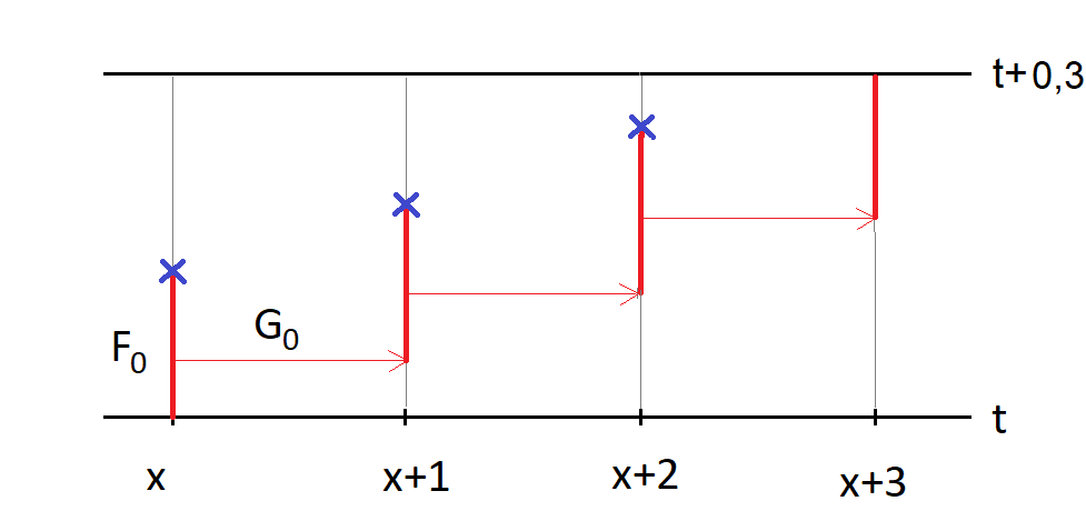
Figure 4. Illustration of a horizontal crossing inside the box $B_{h}(t,x)$. The red lines indicate the infection path, the red arrows indicate the transmissions and the X marks indicate the cures, $F_{0}=F_{0}^{(t)}(a)$ and $G_{0}=G_{0}^{(t)}(a)$.

Since $a_{0}>0$, we can fix $\lambda_{h}$ such that $P(\exp(\lambda_{h})\leq a_{0})=(1-\epsilon)^{\frac{1}{6}}$, which is equivalently to fix $\lambda_{h}=\frac{-1}{a_{0}}\log(1-[1-\epsilon]^{\frac{1}{6}})$. With this value of $\lambda_{h}$ we have

$$P\Big{(}G_{i}^{(s_{i})}(a_{0})\Big{|}F_{i}^{(s_{i})}(a_{0})\Big{)}=(1-\epsilon)^{\frac{1}{6}}$$

and consequently:

$$\inf_{t\geq 0}\underline{\mathbb{P}}_{t}^{\mu}(C_{h}(x,t))\geq\prod_{i=0}^{2}\left[P\Big{(}G_{i}^{(s_{i})}(a_{0})\Big{|}F_{i}^{(s_{i})}(a_{0})\Big{)}\inf_{s_{i}\geq 0}\underline{\mathbb{P}}_{s_{i}}^{\mu}\Big{(}F_{i}^{(s_{i})}(a_{0})\Big{)}\right]$$

$$\geq\left[(1-\epsilon)^{\frac{1}{6}}(1-\epsilon)^{\frac{1}{6}}\right]^{3}=1-\epsilon.\ \ \ \ \ \vspace{-0.5cm}$$

∎

Lemma 3.5.

Let $B_{v}(x,t)=[x,x+1]\times[t,t+1]$ be a space-time box that we will call “vertical box” and fix $\epsilon\in(0,1)$. Assuming that the vertex $x$ or $x+1$ is infected at time $t$, denote by $C_{v}(x,t)$ the event $\{$the infection survives up to time $t+1$ inside $B_{v}(x,t)\}$ and when it happens we will say that we have a vertical crossing of the box $B_{v}(x,t)$. Then uniformly on $\tau$, for any $x$ and considering the RCP($\mu$), there exists $\lambda_{v}=\lambda_{v}(\epsilon)<\infty$ such that:

$$\inf_{t\geq 0}\underline{\mathbb{P}}_{t}^{\mu}(C_{v}(x,t))\geq 1-\epsilon,\ \mbox{if}\ \lambda>\lambda_{v}.$$

Proof.

(Lemma 3.5) Suppose without loss of generality that only the vertex $x$ is infected at time $t$ and that $\mathcal{R}\cap[t,t+1]\neq\emptyset$, since the occurrence of $C_{v}(x,t)$ would be trivial without this last assumption.

Note that since the box $B_{v}(x,t)$ has only two vertices, the infection has to keep jumping between these two vertices until time $t+1$. In Figure 5 we have an illustration of event $C_{v}(x,t)$ occurring.

So, our strategy will be the following: First, we will look to the cure marks of vertices $x$ and $x+1$ inside the box $B_{v}(x,t)$ and say that these marks are “good” if they satisfy an event $A_{t}$ that will be explained later. Then we can write:

$$\inf_{t\geq 0}\underline{\mathbb{P}}_{t}^{\mu}(C_{v}(x,t))=\inf_{t\geq 0}\Big{[}P(C_{v}(x,t)|A_{t})\underline{\mathbb{P}}_{t}^{\mu}(A_{t})+P(C_{v}(x,t)|A_{t}^{c})\underline{\mathbb{P}}_{t}^{\mu}(A_{t}^{c})\Big{]}$$

$$\geq\inf_{t\geq 0}P(C_{v}(x,t)|A_{t})\underline{\mathbb{P}}_{t}^{\mu}(A_{t}).\qquad\qquad$$

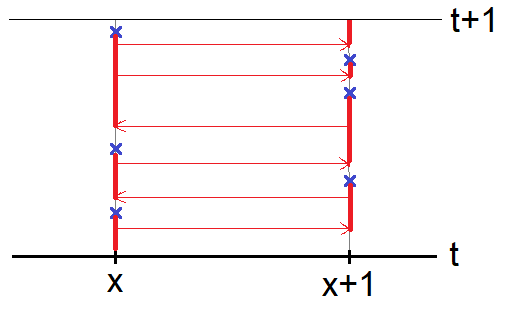
Figure 5. Illustration of a vertical crossing inside the box $B_{v}(x,t)$. The red lines indicate the infection path, the red arrows indicate the transmissions and the X marks indicate the cures.

After that, we will say that the attempt of transmissions inside the box $B_{v}(x,t)$ are “good” if they satisfy an event $V$ that will be explained later. This event $V$ will be chosen such that the occurrence of $A_{t}$ and $V$ together guarantee the occurrence of $C_{v}(x,t)$. An important detail here is that since the cure marks are independent of the transmission attempts, then the event $A_{t}$ will depend only on the distribution of the cure times, and the event $V$ given $A_{t}$ will depend only on the distribution of infection times.

To begin let $S_{i}$ and $\tilde{S}_{i}$ be the time of the $i-th$ cure mark of vertex $x$ and $x+1$ inside the box $B_{v}(x,t)$ respectively. Also, let $N$ and $\tilde{N}$ denote the number of renewal marks of the processes $\mathcal{R}_{x}$ and $\mathcal{R}_{x+1}$ inside the box $B_{v}(x,t)$ respectively. Now fix $p_{1}=1-(1-\epsilon)^{\frac{1}{4}}$. By Lemmas 3.1 and 3.2 there exists $w_{0}=w_{0}(p_{1})$ such that:

$$\inf_{t\geq 0}\underline{\mathbb{P}}_{t}^{\mu}(S_{1}\geq t+w_{0})\geq 1-p_{1}=(1-\epsilon)^{\frac{1}{4}}.$$ (3.6)

From now on fix $w_{0}$ as the biggest value that satisfies (3.6). Then, by Lemma 3.3 there exists $v_{0}=v_{0}(p_{0})$ such that for any $t\geq 0$:

$$\inf_{t\geq 0}\underline{\mathbb{P}}_{t}^{\mu}\Big{(}\min_{1\leq i\leq N}\min_{1\leq j\leq\tilde{N}}\left|\tilde{S}_{j}-S_{i}\right|\geq v_{0},\Big{|}S_{1}\geq t+w_{0}\Big{)}\geq 1-p_{1}=(1-\epsilon)^{\frac{1}{4}}.$$ (3.7)

From now on, fix $v_{0}$ as the biggest value that satisfies (3.7). At this point, we will define the event $A_{t}$, which identifies if the cure marks are “good” or not. Let $A_{t}=A^{(t)}_{1}\cap A^{(t)}_{2}$ where:

$$A_{1}^{(t)}=\Big{\{}\min_{1\leq i\leq N}\min_{1\leq j\leq\tilde{N}}\left|\tilde{S}_{j}-S_{i}\right|\geq v_{0}\Big{\}},\qquad A_{2}^{(t)}=\Big{\{}S_{1}\geq t+w_{0}\Big{\}}.$$

Then, by (3.6) and (3.7) we have that

$$\inf_{t\geq 0}\underline{\mathbb{P}}_{t}^{\mu}(A_{t})\geq\inf_{t\geq 0}\underline{\mathbb{P}}_{t}^{\mu}\Big{(}A_{1}^{(t)}\mid A_{2}^{(t)}\Big{)}.\inf_{t\geq 0}\underline{\mathbb{P}}_{t}^{\mu}\Big{(}A_{2}^{(t)}\Big{)}\geq(1-\epsilon)^{\frac{1}{4}}(1-\epsilon)^{\frac{1}{4}}=(1-\epsilon)^{\frac{1}{2}}.$$

Now define a sequence of $M+2$ increasing times $(\tau_{i})_{i\geq 0}$ inside $[t,t+1]$ in the following way: $\tau_{0}=t$, $\tau_{1}=S_{1}$, $\tau_{i}=\min\{\mathcal{R}_{x+1}\cap(\tau_{i-1},\infty)\}$ for $i$ even and $\tau_{i}=\min\{\mathcal{R}_{x}\cap(\tau_{i-1},\infty)\}$ for $i>1$ odd. Continue this construction until $\tau_{i}\leq t+1$. Then, set $M=\max\{i\geq 1;\tau_{i}\leq t+1\}$ and $\tau_{M+1}=t+1$.

Recall that $(\mathcal{N}_{x,y})_{(x,y)\in\mathcal{E}}$ denote the Poisson processes that describe the times when the vertex $x$ tries to infect $y$. Then, we can define $(H_{i}^{(t)})_{i\geq 1}$ the event $\{$the infection reaches time $\tau_{i}$ inside the box $B_{v}(x,t)$ given that it reached time $\tau_{i-1}\}$. Note that $P(H_{1}^{(t)})=P(H_{M+1}^{(t)})=1$ for any $t\geq 0$. Besides that, since $\mathcal{N}_{x,y}$ has the same distribution of $\mathcal{N}_{y,x}$, then for $2\leq i\leq M$,

$$P\Big{(}H_{i}^{(t)}\Big{)}=P(\mathcal{N}_{x,x+1}\cap(\tau_{i-1},\tau_{i}]\neq\emptyset).$$

Denote by $u_{0}=w_{0}\wedge v_{0}$. Given the occurrence of $A_{t}$, we have $|\tau_{i}-\tau_{i-1}|\geq u_{0}$ for every $i=1,\ldots,M$ and consequently, the sequence $(H_{i}^{(t)})_{i\geq 1}$ will have at most $\lceil(u_{0})^{-1}\rceil+1$ events. If all these events occur, then we guarantee that $C_{v}(x,t)$ occurs. Recalling that the transmissions times are given by Poisson processes with parameter $\lambda$ and denoting by $(Y_{i})_{i\geq 1}$ a sequence of i.i.d random variables with distribution $\exp(\lambda)$, we have that for any $i=2\ldots,M$:

$$\inf_{t\geq 0}P\Big{(}H_{i}^{(t)}\Big{|}A_{t}\Big{)}\geq P(Y_{i}\leq u_{0})=1-e^{-\lambda u_{0}}.$$

Now define $V$ the event $\{\max_{2\leq i\leq\lceil(u_{0})^{-1}\rceil}Y_{i}\leq u_{0}\}$. Since we have the Markov property on the transmissions,

$$\inf_{t\geq 0}P(C_{v}(x,t)|A_{t})\geq\inf_{t\geq 0}P\Big{(}\bigcap_{i=1}^{M+1}H_{i}^{(t)}\Big{|}A_{t}\Big{)}=\inf_{t\geq 0}\prod_{i=1}^{M+1}P\Big{(}H_{i}^{(t)}|A_{t}\Big{)}\geq P\Big{(}H_{1}^{(0)}\Big{)}P(V)P\Big{(}H_{M+1}^{(0)}\Big{)}$$

$$\ \geq(1-e^{-\lambda u_{0}})^{\lceil(u_{0})^{-1}\rceil-1}.\qquad\qquad\qquad\qquad\qquad\qquad\qquad$$

So, taking $\lambda_{v}=\frac{-1}{u_{0}}\log\left(1-[1-\epsilon]^{\frac{1}{2\lceil(u_{0})^{-1}\rceil-2}}\right)$, we have $\inf_{t\geq 0}P(C_{v}(x,t)|A_{t})\geq(1-\epsilon)^{\frac{1}{2}}$ and hence,

$$\inf_{t\geq 0}\underline{\mathbb{P}}_{t}^{\mu}(C_{v}(x,t))\geq\inf_{t\geq 0}P(C_{v}(x,t)|A_{t})\underline{\mathbb{P}}_{t}^{\mu}(A_{t})\geq(1-\epsilon)^{\frac{1}{2}}(1-\epsilon)^{\frac{1}{2}}=1-\epsilon.$$

Then, for any $\lambda>\lambda_{v}$ we have $\inf_{t\geq 0}P(C_{v}(x,t))\geq 1-\epsilon$. ∎

Now we are finally ready to present the proof of Theorem 1.2.

Proof.

(Theorem 1.2) Consider a graph $G$ in $\mathbb{Z}^{2}_{0\leq x\leq y+1}$ with oriented edges $z+(1,0)$ and $z+(0,1)$. Define a bond percolation model in $G$ by stating that a horizontal edge from $(x,y)$ to $(x+1,y)$ is open if we have a horizontal crossing (as defined in Lemma 3.4) of the box $B_{h}(2x,y)$ in the RCP($\mu$) and that a vertical edge from $(x,y)$ to $(x,y+1)$ is open if we have a vertical crossing (as defined in Lemma 3.5) of the box $B_{v}(2x,y)$ in the RCP($\mu$). When this model percolates, the associated RCP($\mu$) will survive.

Note that this percolation model exhibits long range dependency in the second coordinate since the positions of the cure marks in the associated RCP are non-markovian. But by Lemma 3.4, if we take $\lambda>\lambda_{h}$, then the probability that an edge of $G$ from $(x,y)$ to $(x+1,y)$ is open, given any possible configurations of the other edges with second coordinate smaller than $y$, is greater than $1-\epsilon$. Besides that, looking at the horizontal edges with the same second coordinate, only those that share one of the extremities are not independent (since the associated boxes will not be disjoint).

Now, looking at the vertical edges, if we take $\lambda>\lambda_{v}$, then the probability that an edge of $G$ from $(x,y)$ to $(x,y+1)$ is open, given any possible configurations of the other edges with second coordinate smaller than $y$, is greater than $1-\epsilon$ by Lemma 3.5. Besides that, vertical edges that are not in the same vertical line are independent of each other.

Take $\lambda_{0}=\lambda_{h}\vee\lambda_{v}$. These previous facts allow us to conclude that this percolation model is dominated from below by the random field with density $\rho$ and that we can make the density of these random fields become arbitrarily close to $1$ if we take $1-\epsilon$ large enough (see [10] for instance). Then, if we fix $\epsilon$ small enough, the RCP($\mu$) survives with positive probability for any $\lambda>\lambda_{0}$.
∎

References

- [1] R. Durrett: Ten Lectures on particle systems. (Ecole d’Eté de Probabilités de Saint-Flour XXIII, 1993) Lecture Notes in Math., 1608, 97–201, Springer, Berlin (1995)
- [2] L. R. Fontes, D.H.U. Marchetti, T.S. Mountford, M. E. Vares: Contact process under renewals I. Stoch. Proc. Appl., 129(8), 2903–2911 (2019).
- [3] L.R. Fontes, P. Gomes, R. Sanchis: Contact process under heavy-tailed renewals on finite graphs. Bernoulli, 27(3), 1745–1763 (2020).
- [4] L. R. Fontes, T.S. Mountford, M. E. Vares: Contact process under renewals II. Stoch. Proc. Appl., 130(2), 1103–1118 (2020).
- [5] L. R. Fontes, T.S. Mountford, D. Ungaretti, M. E. Vares: Renewal Contact Processes: phase transition and survival. Stoch. Proc. Appl., 161, 102–136 (2023).
- [6] T. E. Harris: Contact interactions on a lattice. The Annals of Probability, 2(6) 969–988 (1974)
- [7] T. E. Harris: Aditive Set-Valued Markov Process and Graphical Methods. The Annals of Probability, 6(3) 355–378 (1978)
- [8] M. Hilário, D. Ungaretti, D. Valesin, M. E. Vares: Results on the contact process with dynamic edges or under renewals. Electron. J. Probab. 27 article no. 91, 31pp (2022).
- [9] T. M. Liggett: Interacting Particle Systems. Grundlehren der Mathematischen Wissenschaften 276, New York: Springer (1985)
- [10] T. Liggett, R. Schonmann, A. Stacey: Domination by product measures. The Annals of Probability, 25(1), 71-95 (1997)