FedDec: Peer-to-peer Aided Federated Learning

Abstract

Federated learning (FL) has enabled training machine learning models exploiting the data of multiple agents without compromising privacy. However, FL is known to be vulnerable to data heterogeneity, partial device participation, and infrequent communication with the server, which are nonetheless three distinctive characteristics of this framework. While much of the recent literature has tackled these weaknesses using different tools, only a few works have explored the possibility of exploiting inter-agent communication to improve FL’s performance. In this work, we present FedDec, an algorithm that interleaves peer-to-peer communication and parameter averaging (similar to decentralized learning in networks) between the local gradient updates of FL. We analyze the convergence of FedDec under the assumptions of non-iid data distribution, partial device participation, and smooth and strongly convex costs, and show that inter-agent communication alleviates the negative impact of infrequent communication rounds with the server by reducing the dependence on the number of local updates $H$ from $O(H^{2})$ to $O(H)$. Furthermore, our analysis reveals that the term improved in the bound is multiplied by a constant that depends on the spectrum of the inter-agent communication graph, and that vanishes quickly the more connected the network is. We confirm the predictions of our theory in numerical simulations, where we show that FedDec converges faster than FedAvg, and that the gains are greater as either $H$ or the connectivity of the network increase.

1 Introduction

Federated learning (FL) is a recent machine learning framework that allows multiple agents, each of them with their own dataset, to train a model collaboratively without sharing their data [1, 2, 3, 4]. The federated setting assumes that all agents are connected to a server that can communicate with each of them and that is in charge of aggregating the agents’ updates to obtain the global model. This is similar to parallel distributed (PD) model training [5, 6, 7, 8], with one crucial difference: in the latter, the agents send gradients to the central server to update the parameter value with a gradient step, while in FL the agents send their own local parameters for the server to average them. This has an impact on the communication frequency required by each framework: in PD one round of communication between (usually all) the agents and the server has to happen every time a (mini-batch) stochastic gradient descent (SGD) step is taken at the nodes, while in FL (i) multiple SGD updates can happen before a new server communication round takes place (which in FL literature are usually called local updates), and (ii) not all devices need to engage in the server communication round (which is known as partial participation). This makes FL a much more suitable option for settings with a large number of agents and a limited communication bandwidth with the server.

In contrast to the approaches described above, the decentralized setting does not rely on a central server for the aggregation of the nodes’ updates. Instead, it assumes that the agents are interconnected in a network and each of them can exchange optimization values (either parameters or gradients, depending on the algorithm) with its direct neighbors [9, 10, 11, 12, 13, 14, 15]. In the decentralized setting, every node performs an averaging step of all its neighbors’ received values before taking a new gradient step. Algorithms for this setting are designed such that the local parameters of all nodes converge to the global minimizer, while in FL it is the central server who keeps track of the most recent parameter value and broadcasts it to all agents every once in a while.

The attractive feature of FL of allowing to have server communication rounds every once in a while comes at a cost: the more infrequent the server communication rounds are (i.e., the more local updates are performed at the agents), the slower is the convergence [16, 17]. For this reason, in this paper we propose to exploit inter-agent communication to reduce the negative impact of infrequent server communication rounds. Given that (i) each agent is expected to have much fewer neighbors than the total number of agents, and (ii) short-range inter-agent communications allow for spectrum reuse, agents can communicate much more often between them than with the server [18, 19].

We propose FedDec, an FL algorithm where the agents can exchange and average their current parameters with those of their neighbors in between the local SGD steps. We show that this modification reduces the dependence of the convergence bound on the number of local SGD steps $H$ from $O(H^{2})$ [16, 20] to $O(H)$ (Theorem 1). Furthermore, we show that, in our analysis, the extra $H$ factor is replaced by a value $\alpha$ that depends on the spectrum of the graph defining the inter-agent communication. Since the value of $\alpha$ quickly decreases as the network becomes more connected, our result indicates that for mildly connected networks $H$ can be increased without severely hurting convergence speed (or conversely, for fixed $H$, FedDec will be faster than FedAvg [1], its counterpart without inter-agent communication).

Peer-to-peer communication within FL has been considered a few times in the past [21, 22, 23, 24, 25]. These works either analyze very general distributed settings that have FL with inter-agent communication as a particular case [24, 25], or show that FL with inter-agent communication converges at the same rate as standard FL, and outperforms it in simulations [21, 22, 23]. However, none of them has characterized analytically how inter-agent communication reduces the impact of local updates on convergence, and in particular, how this reduction depends on the inter-agent connectivity.

Our contributions can be summarized as follows:

• We introduce FedDec, an FL algorithm where the agents can average their parameters with those of their neighbors in between the SGD steps. Our model accounts for failures in the inter-agent communication links, so that only a few (or even none) of the parameters of a node’s neighbors may be averaged at some iterations.

• We prove that, for non-iid data, partial device participation, and smooth and strongly convex objectives, FedDec converges at the $O(1/T)$ rate (where $T$ is the total number of iterations executed) of FL algorithms that do not account for inter-agent communication [16, 20], but improves the dependence on the number of local updates $H$ from $O(H^{2})$ to $O(H)$.

• Furthermore, we show that the improved term is multiplied by a quantity that depends on the spectrum of the inter-agent communication network, and which quickly vanishes the more connected the network is.

• We support our theoretical findings with numerical simulations, where we confirm that the performance of FedDec with respect to FedAvg [1] increases with both $H$ and the connectivity of the network.

2 System Model and the FedDec Algorithm

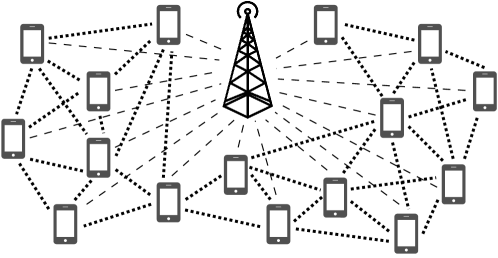
Figure 1: The FedDec setting. Peer-to-peer communication links are shown in dotted lines (high-bandwidth links). Communication links between the agents and the server are shown in dashed lines (low-bandwidth links).

We consider a system where $n$ agents can exchange messages with a central server and also with some other nearby agents. We assume that the inter-agent communication links may fail at some iterations (e.g. due to outage), but when all links are active the agents form a connected network (see Figure 1). Each node $i\in[n]$ has a local cost $F_{i}:\mathbb{R}^{d}\rightarrow\mathbb{R}$,

$$F_{i}({\mathbf{z}}):=\mathbb{E}_{\psi_{i}\sim\mathcal{D}_{i}}F_{i}({\mathbf{z}},\psi_{i}),$$

where $\mathcal{D}_{i}$ can be an underlying local data distribution from where new samples (or mini-batches) are drawn each time an SGD step is taken, or the uniform distribution over a static dataset. Note that the $\mathcal{D}_{i}$ can be different at each node. The objective of the nodes and the server is to find the minimizer

$${\mathbf{z}}^{*}:=\operatorname*{argmin}_{{\mathbf{z}}\in\mathbb{R}^{d}}f({\mathbf{z}}),\qquad f({\mathbf{z}}):=\frac{1}{n}{\sum_{i=1}^{n}}F_{i}({\mathbf{z}})$$

under the constraints that nodes can only communicate with their direct neighbors (high-bandwidth links) and every once in a while they can get a request from the server to send their current parameter values (low-bandwidth links). In wireless settings, these capacities are imposed by the shared nature of the cellular medium. While the communication with the server is constrained by the bandwidth available, device-to-device communications in the short range allows for spectrum reuse, and thus for higher throughput [18, 19].

At each server communication round, the server samples the devices uniformly at random with replacement to form an index pool $\mathcal{S}_{t}$ of devices that it will poll during that round. We assume $|\mathcal{S}_{t}|=K\;\forall\,t$. It then averages the parameters of all $j\in\mathcal{S}_{t}$ and broadcasts the new value to all nodes in the network. Due to the limited bandwidth, we assume partial participation, i.e. $K\ll n$. We assume that the server aggregation rounds happen every $H$ local updates, and we call $\mathcal{H}=\{t:t\text{ modulo }H=0\}$ the set of those times.

One local update of FedDec for a node $i$ consists on (i) taking an SGD step, (ii) for all active links (i.e. $\forall j{:}\,W^{t}_{ij}>0$), exchanging the new parameter value with its neighbors, and (iii) combining all new values (including its own) with weights $W^{t}_{ij}$ to form the new iterate. We call this algorithm FedDec, and the precise steps are shown in Algorithm 1.

Algorithm 1 Peer-to-peer aided FL (FedDec)

1:  Initialize ${\mathbf{z}}_{i}^{1}={\mathbf{z}}^{1}\;\forall i\in[n]$ and let $\eta_{t}=\frac{2}{\mu(t+\gamma)}$.

2:  for $t=1,\ldots,T$ all agents $i\in[n]$ do

3:     Sample mixing matrix $W^{t}\sim\mathcal{W}$

4:     Sample mini-batch $\xi_{i}^{t}$ and compute $\nabla F_{i}({\mathbf{z}}_{i}^{t},\xi_{i}^{t})$

5:     Update local parameter ${\mathbf{x}}_{i}^{t+\frac{1}{2}}={\mathbf{z}}_{i}^{t}-\eta_{t}\nabla F_{i}({\mathbf{z}}_{i}^{t},\xi_{i}^{t})$

6:     Average with neighbors ${\mathbf{x}}_{i}^{t+1}=\sum_{j=1}^{n}W^{t}_{ij}{\mathbf{x}}_{j}^{t+\frac{1}{2}}$

7:     If $t+1\in\mathcal{H}$ then

8:        Server samples $\mathcal{S}_{t}=\{j_{\ell}:j_{\ell}\sim\mathcal{U}([n])\}_{\ell=1}^{K}$

9:        it computes ${\mathbf{z}}^{t+1}=\frac{1}{K}\sum_{\ell=1}^{K}{\mathbf{x}}_{j_{\ell}}^{t+1}$

10:        and broadcasts so that ${\mathbf{z}}_{i}^{t+1}={\mathbf{z}}^{t+1}\;\forall i\in[n]$

11:     otherwise

12:        ${\mathbf{z}}_{i}^{t+1}={\mathbf{x}}_{i}^{t+1}$

13:  end for

14:  Output ${\mathbf{z}}^{T+1}$

With slight abuse of notation, the stochastic gradient of a node $i$ computed on a mini-batch $\xi_{i}=\{\psi_{i}^{j}:\psi_{i}^{j}\sim\mathcal{D}_{i}\}_{j=1}^{m}$ of size $m$ is given by $\nabla F_{i}({\mathbf{z}}_{i},\xi_{i})=\frac{1}{m}\sum_{j=1}^{m}\nabla F_{i}({\mathbf{z}}_{i},\psi_{i}^{j})$. For simplicity, we will assume that the number of iterations $T$ satisfies $(T$ modulo $H)=0$, so that the outputted value in Alg. 1 is the current parameter at all nodes. We will also take the following assumptions, which are standard in the literature [14, 20, 16, 22, 23, 21].

Assumption 1.

We assume the following $\forall F_{i}({\mathbf{z}}),i\in[n]$:

1) $L$-smoothness and $\mu$-strong convexity:

$$F_{i}({\mathbf{y}}) \leq F_{i}({\mathbf{x}})+{\left\langle\nabla F_{i}({\mathbf{x}}),{\mathbf{y}}-{\mathbf{x}}\right\rangle}+(L/2){\left\lVert{\mathbf{y}}-{\mathbf{x}}\right\rVert_{2}^{2}},$$ (1)

$$F_{i}({\mathbf{y}}) \geq F_{i}({\mathbf{x}})+{\left\langle\nabla F_{i}({\mathbf{x}}),{\mathbf{y}}-{\mathbf{x}}\right\rangle}+(\mu/2){\left\lVert{\mathbf{y}}-{\mathbf{x}}\right\rVert_{2}^{2}}.$$ (2)

2) Bounded variance of the local gradients:

$$\mathbb{E}{\left\lVert\nabla F_{i}({\mathbf{x}},\xi_{i})-\nabla F_{i}({\mathbf{x}})\right\rVert}_{2}^{2}\leq\sigma_{i}^{2}.$$

3) Bounded energy of the local gradients:

$$\mathbb{E}{\left\lVert\nabla F_{i}({\mathbf{x}},\xi_{i})\right\rVert}_{2}^{2}\leq G^{2}\text{ for }i\in[n].$$ (3)

We remark that (2) implies ${\left\lVert\nabla F_{i}({\mathbf{z}}_{i})\right\rVert}_{2}\geq\mu{\left\lVert{\mathbf{z}}_{i}-{\mathbf{z}}_{i}^{*}\right\rVert}_{2}$ (see definition of ${\mathbf{z}}_{i}^{*}$ below). Therefore, in order to satisfy (3) we must additionally assume that the parameter iterates ${\mathbf{z}}_{i}$ belong to a bounded set throughout the iterations.

Note that $L$-smoothness implies

$${\left\lVert\nabla F_{i}({\mathbf{x}})-\nabla F_{i}({\mathbf{y}})\right\rVert}\leq L{\left\lVert{\mathbf{x}}-{\mathbf{y}}\right\rVert}_{2},$$ (4)

$${\left\lVert\nabla f({\mathbf{z}})\right\rVert_{2}^{2}}{\,=\,}{\left\lVert\nabla f({\mathbf{z}}){-}\nabla f({\mathbf{z}^{*}})\right\rVert}_{2}^{2}{\,\leq\,}2L(f({\mathbf{z}}){-}f({\mathbf{z}^{*}})).$$ (5)

Furthermore, the local gradient’s bounded variance implies

$$\mathbb{E}{\left\lVert\frac{1}{n}{\sum_{i=1}^{n}}{\left(\nabla F_{i}({\mathbf{z}}_{i}^{t})-\nabla F_{i}({\mathbf{z}}_{i}^{t},\xi_{i}^{t})\right)}\right\rVert}_{2}^{2}\leq\frac{{\overline{\sigma}}^{2}}{n},$$ (6)

with ${\overline{\sigma}}^{2}=\frac{1}{n}{\sum_{i=1}^{n}}\sigma_{i}^{2}$.

We quantify the degree of heterogeneity (or non-iidness) between the local functions through the quantity

$$\Gamma=\frac{1}{n}{\sum_{i=1}^{n}}(F_{i}({\mathbf{z}^{*}})-F_{i}({\mathbf{z}}_{i}^{*})),\text{ where }\;{\mathbf{z}}_{i}^{*}=\operatorname*{argmin}_{{\mathbf{z}}}F_{i}({\mathbf{z}}).$$

FedDec uses two parameters to track the updates, ${\mathbf{z}}_{i}$ and ${\mathbf{x}}_{i}$ (see Alg. 1). We define

$${\overline{{\mathbf{x}}}}^{t}=\frac{1}{n}\sum_{i=1}^{n}{\mathbf{x}}_{i}^{t},\qquad{\overline{{\mathbf{z}}}}^{t}=\frac{1}{n}\sum_{i=1}^{n}{\mathbf{z}}_{i}^{t},$$

which will be useful in the analysis. Note that ${\overline{{\mathbf{z}}}}^{t}={\overline{{\mathbf{x}}}}^{t}$ only when $t\notin\mathcal{H}$. Otherwise, if $t\in\mathcal{H}$, we have that the equality holds only in expectation:

$$\mathbb{E}_{\mathcal{S}_{t}}{\overline{{\mathbf{z}}}}^{t}=\mathbb{E}_{\mathcal{S}_{t}}\frac{1}{n}{\sum_{i=1}^{n}}{\mathbf{z}}_{i}^{t}=\frac{1}{n}{\sum_{i=1}^{n}}\frac{1}{K}\sum_{\ell=1}^{K}\mathbb{E}_{\mathcal{S}_{t}}{\mathbf{x}}_{j_{\ell}}^{t}={\overline{{\mathbf{x}}}}^{t}.$$ (7)

Lastly, we assume the following about the $W^{t}=\{W^{t}_{ij}\}$.

Assumption 2.

The averaging matrices $W^{t}\in\mathbb{R}^{n\times n}$ are iid random variables drawn from a distribution $\mathcal{W}$ of matrices that (i) are symmetric, (ii) are doubly stochastic, and (iii) have $W^{t}_{ij}\geq 0$ if agents $i$ and $j$ are connected and $W^{t}_{ij}=0$ otherwise. Note that this implies that $\forall\,W\in\mathcal{W}:W\mathbf{1}=\mathbf{1}$, $\mathbf{1}^{T}W=\mathbf{1}^{T}$. Additionally, we require that the eigenvalues of $\mathbb{E}_{W}{\left[WW^{T}\right]}$ satisfy $1=\lambda_{1}>{\left|\lambda_{2}\right|}\geq\ldots\geq{\left|\lambda_{n}\right|}$.

In the next section we prove that FedDec converges as $O(1/T)$, similarly to other FL algorithms taking the same assumptions, but it reduces the negative impact of local updates by replacing an $H^{2}$ factor [16, 20], with $H\alpha$, where $\alpha$ is a quantity that decreases quickly as the inter-agent communication network becomes more connected.

3 Convergence Analysis

The following theorem establishes the convergence rate of FedDec and constitutes our main result.

Theorem 1.

Under Assumptions 1, 2, and for diminishing stepsize $\eta_{t}=\frac{2}{\mu(\gamma+t)}$, FedDec in Algorithm 1 converges as

$$\mathbb{E}[f({\overline{{\mathbf{z}}}}^{t})]-f({\mathbf{z}^{*}})\leq\frac{L}{\gamma+t}{\left(\frac{2B}{\mu^{2}}+\frac{(\gamma+1)}{2}{\left\lVert{\mathbf{z}}^{1}-{\mathbf{z}^{*}}\right\rVert_{2}^{2}}\right)}$$

where

$$\gamma=\max\{8(L/\mu)-1,H\}$$

$$B={\left(4/K+8\right)}\alpha HG^{2}+6L\Gamma+{\overline{\sigma}}^{2}/n$$

$$\alpha=|\widehat{\lambda}_{2}|\,/\,(1-|\widehat{\lambda}_{2}|)$$

and $|\widehat{\lambda}_{2}|=|\lambda_{2}{\left(\mathbb{E}_{W}{\left[WW^{T}\right]}\right)}|$.

The theorem shows that factors like the energy and the variance of the local gradients, the heterogeneity of the local functions, and the distance of the starting point to the optimum all slow down convergence, which are known facts. However, this bound also shows how inter-agent communication partially mitigates the negative impact of local updates: the term where $H$ appears decreases with $\alpha$, and therefore decreases very fast with $|\widehat{\lambda}_{2}|$ (see Figure 2).

Note that if all inter-agent communication links are assumed to be always active, then $W^{t}=W$ is a fixed matrix and $|\widehat{\lambda}_{2}|={\left|\lambda_{2}\right|}^{2}$. For any given heuristic to construct $W$ (e.g. based on the Laplacian of the graph [26]), the value of ${\left|\lambda_{2}\right|}$ is, in general, lower the more connected the network is (see Table 1 in Section 4). Therefore, the more densely connected the network is, the faster FedDec is expected to converge. In fact, the averaging weights $W_{ij}$ can be designed in order to minimize ${\left|\lambda_{2}\right|}$ (and thus maximize the speedup from inter-agent communication) using eigenvalue optimization techniques [27].

Comparing the bound of Theorem 1 with that of Theorem 2 in [16], obtained for the same setting but without allowing inter-agent communication, we note that the dependence of the first term in $B$ on the number of local iterations $H$ drops from $O(H^{2})$ in [16] to $O(H)$ in our theorem. This suggests that the peer-to-peer communication of FedDec reduces the impact of the infrequent communication rounds with the server, and thus its convergence should be less affected than that of FedAvg as $H$ increases. We verify this behavior in our simulations in Section 4.

To prove the theorem, we will need to bound the quantity ${\left\lVert{\overline{{\mathbf{z}}}}^{t}-{\mathbf{z}^{*}}\right\rVert_{2}^{2}}$. For this we will decompose the term and bound ${\left\lVert{\overline{{\mathbf{z}}}}^{t}-{\overline{{\mathbf{x}}}}^{t}\right\rVert_{2}^{2}}$ and ${\left\lVert{\overline{{\mathbf{x}}}}^{t}-{\mathbf{z}^{*}}\right\rVert_{2}^{2}}$ separately. The following lemmas present these intermediate results, and we prove Theorem 1 at the end of the section. The proofs of the lemmas are given in Appendix B.

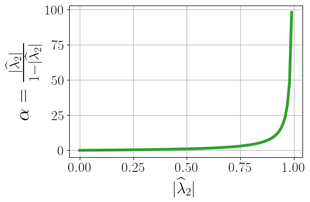
Figure 2: Dependence of $\alpha$ with $|\widehat{\lambda}_{2}|$. For networks moderately connected (see Section 4) we can expect that $\alpha\ll H$, and thus also that FedDec will be faster than FedAvg.

Lemma 2.

For FedDec with stepsize $\eta_{t}\leq\frac{1}{4L}$ it holds

$$\mathbb{E}{{\left\lVert{\overline{{\mathbf{x}}}}^{t+1}-{\mathbf{z}^{*}}\right\rVert_{2}^{2}}}\leq(1-\mu\eta_{t})\mathbb{E}{\left\lVert{\overline{{\mathbf{z}}}}^{t}-{\mathbf{z}^{*}}\right\rVert}_{2}^{2}+\frac{2}{n}\mathbb{E}{\sum_{i=1}^{n}}{\left\lVert{\mathbf{z}}_{i}^{t}-{\overline{{\mathbf{z}}}}^{t}\right\rVert_{2}^{2}}+6L\eta_{t}^{2}\Gamma+\eta_{t}^{2}\frac{{\overline{\sigma}}^{2}}{n}.$$

Lemma 2 bounds the one-step progress of the algorithm before a potential server aggregation round.

Lemma 3.

For stepsizes satisfying $\eta_{t}\leq 2\eta^{t+H}$, it holds that

$$\mathbb{E}{\sum_{i=1}^{n}}{\left\lVert{\mathbf{z}}_{i}^{t}-{\overline{{\mathbf{z}}}}^{t}\right\rVert}_{2}^{2}\leq\eta_{t}^{2}4\alpha HnG^{2}.$$

with $\alpha=\frac{|\widehat{\lambda}_{2}|}{1-|\widehat{\lambda}_{2}|}$.

Lemma 3 bounds the divergence of the local parameters to their average, which increases through the $H$ iterations in between the server broadcasting rounds. It is in this process (which involves multiple neighbor averaging steps) where we see the impact of the connectivity of the graph.

As remarked in Section 2, ${\overline{{\mathbf{z}}}}^{t}={\overline{{\mathbf{x}}}}^{t}\,\forall\,t\notin\mathcal{H}$. Otherwise, the equality holds only in expectation (eq. (7)). Lemma 4 bounds the variance of ${\overline{{\mathbf{z}}}}$ in the latter case.

Lemma 4.

For $t\in\mathcal{H}$ and stepsizes satisfying $\eta_{t}\leq 2\eta_{t+H}$

$$\mathbb{E}{\left\lVert{\overline{{\mathbf{x}}}}^{t}-{\overline{{\mathbf{z}}}}^{t}\right\rVert_{2}^{2}}\leq\frac{1}{K}\eta_{t}^{2}4\alpha HG^{2},$$

with $\alpha$ given in Lemma 3.

Lastly, we have the following lemma from [16].

Lemma 5.

Let a sequence $\Delta^{t}$ satisfy

$$\Delta^{t+1}\leq(1-\mu\eta_{t})\Delta^{t}+\eta_{t}^{2}B$$ (8)

with $\mu,B>0$. Then, for a diminishing stepsize $\eta_{t}=\frac{2}{\mu(\gamma+t)}$ with $\gamma>0$, it holds that $\Delta_{t}\leq\frac{v}{\gamma+t}$, where $v=\max\{\frac{4B}{\mu^{2}},(\gamma+1)\Delta_{1}\}$.

Proof.

See proof of Theorem 1 in [16]. ∎

This bound establishes the parameter choices that allow the sequence $\Delta^{t}$ to converge. We have now all the tools necessary to prove the main theorem.

Proof of Theorem 1.

We start by noting that

$$\mathbb{E}{\left\lVert{\overline{{\mathbf{z}}}}^{t+1}-{\mathbf{z}^{*}}\right\rVert_{2}^{2}} =\mathbb{E}{\left\lVert{\overline{{\mathbf{z}}}}^{t+1}-{\overline{{\mathbf{x}}}}^{t+1}+{\overline{{\mathbf{x}}}}^{t+1}-{\mathbf{z}^{*}}\right\rVert_{2}^{2}}$$

$$=\mathbb{E}{\left\lVert{\overline{{\mathbf{z}}}}^{t+1}-{\overline{{\mathbf{x}}}}^{t+1}\right\rVert_{2}^{2}}+\mathbb{E}{\left\lVert{\overline{{\mathbf{x}}}}^{t+1}-{\mathbf{z}^{*}}\right\rVert_{2}^{2}}+2\mathbb{E}{\left\langle{\overline{{\mathbf{z}}}}^{t+1}-{\overline{{\mathbf{x}}}}^{t+1},{\overline{{\mathbf{x}}}}^{t+1}-{\mathbf{z}^{*}}\right\rangle}.$$

The last term becomes zero when taking expectation, since $\mathbb{E}_{\mathcal{S}_{t}}{\overline{{\mathbf{z}}}}^{t}={\overline{{\mathbf{x}}}}^{t}$ (eq. (7)). The first term is zero when $t+1\notin\mathcal{H}$, and for all other iterations we can bound it using Lemma 4 (and the fact that $\eta_{t+1}^{2}<\eta_{t}^{2}$). We bound the second term using Lemma 2. We have then

$$\mathbb{E}{\left\lVert{\overline{{\mathbf{z}}}}^{t+1}-{\mathbf{z}^{*}}\right\rVert_{2}^{2}}\leq\frac{1}{K}\eta_{t}^{2}4\alpha HG^{2}+(1-\mu\eta_{t})\mathbb{E}{\left\lVert{\overline{{\mathbf{z}}}}^{t}-{\mathbf{z}^{*}}\right\rVert}_{2}^{2}+\frac{2}{n}\mathbb{E}{\sum_{i=1}^{n}}{\left\lVert{\mathbf{z}}_{i}^{t}-{\overline{{\mathbf{z}}}}^{t}\right\rVert_{2}^{2}}+6L\eta_{t}^{2}\Gamma+\eta_{t}^{2}\frac{{\overline{\sigma}}^{2}}{n}.$$

Using Lemma 3 to bound $\mathbb{E}{\sum_{i=1}^{n}}{\left\lVert{\mathbf{z}}_{i}^{t}-{\overline{{\mathbf{z}}}}^{t}\right\rVert_{2}^{2}}$ we get

$$\mathbb{E}{\left\lVert{\overline{{\mathbf{z}}}}^{t+1}-{\mathbf{z}^{*}}\right\rVert_{2}^{2}}\leq(1-\mu\eta_{t})\mathbb{E}{\left\lVert{\overline{{\mathbf{z}}}}^{t}-{\mathbf{z}^{*}}\right\rVert}_{2}^{2}+\eta_{t}^{2}{\left[{\left(\frac{4}{K}+8\right)}\alpha HG^{2}+6L\Gamma+\frac{{\overline{\sigma}}^{2}}{n}\right]}.$$

This has the form of (8) with $\Delta^{t}={\left\lVert{\overline{{\mathbf{z}}}}^{t}-{\mathbf{z}^{*}}\right\rVert_{2}^{2}}$ and $B={\left(\frac{4}{K}+8\right)}\alpha HG^{2}+6L\Gamma+{\overline{\sigma}}^{2}/n$, so applying Lemma 5:

$$\mathbb{E}{\left\lVert{\overline{{\mathbf{z}}}}^{t}-{\mathbf{z}^{*}}\right\rVert_{2}^{2}}\leq\frac{v}{\gamma+t}\leq\frac{1}{\gamma+t}{\left(\frac{4B}{\mu^{2}}+(\gamma+1)\Delta_{1}\right)}.$$ (9)

Note that in order to ensure $\eta_{t}\leq\frac{1}{4L}$ (Lemma 2) and $\eta_{t}\leq 2\eta_{t+H}$ (Lemmas 3 and 4) we need to set $\gamma=\max\{8\frac{L}{\mu}-1,H\}$. Finally, using $L$-smoothness and $\nabla f({\mathbf{z}}^{*})=0$,

$$\mathbb{E}[f({\overline{{\mathbf{z}}}}^{t})]-f({\mathbf{z}^{*}})\leq\frac{L}{2}\mathbb{E}{\left\lVert{\overline{{\mathbf{z}}}}^{t}-{\mathbf{z}^{*}}\right\rVert_{2}^{2}}.$$

Using (9) in the inequality above gives the result. ∎

4 Numerical Results

In this section we compare the performance of FedDec with that of FedAvg [1] in a problem with partial device participation and heterogeneous data.

We consider the linear regression problem

$$F_{i}({\mathbf{z}})=\frac{1}{M}{\left\lVert X_{i}\,{\mathbf{z}}-Y_{i}\right\rVert_{2}^{2}},\qquad i\in[n],$$

with $X_{i},Y_{i}\in\mathbb{R}^{M\times d},M=10$, and $d=25$. For generating the regression data we follow a procedure similar to [12]: we set $[X_{i}]_{j}\sim\mathcal{N}(0,0.25^{2}),\,j\in[d]$ and $Y_{i}=c_{i}(v+\cos(v))$, where $v=X_{i}\mathbf{1}$ and $c_{i}=2^{i},i\in[n]$ is a factor that makes the data at each node significantly different from all others.

For the inter-agent communication, we generate geographic graphs of $n=20$ nodes by taking $n$ points distributed uniformly at random in a $1\times 1$ square and joining with a link all pairs of points whose Euclidean distance is smaller than a radius $r$. We test our algorithms in two graphs with $r=0.35$ and $0.5$, respectively (see Figure 3). We run $T=5000$ iterations with $K=2$, $m=1$, and $H=10,100$.

Figure 4 shows the convergence of FedDec and FedAvg for each graph in Fig. 3 and the two values of $H$. The stepsize was set to the value indicated in Theorem 1. The lines shown are the average of ten independent runs of the algorithms on the same problem instance.

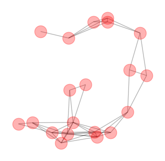
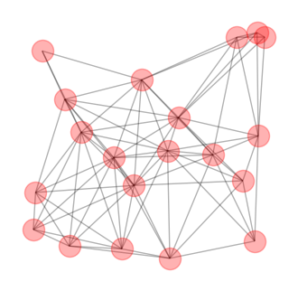
Figure 3: Graphs used in the simulations. Left: sparse graph with $r=0.35$. Right: dense graph with $r=0.5$.

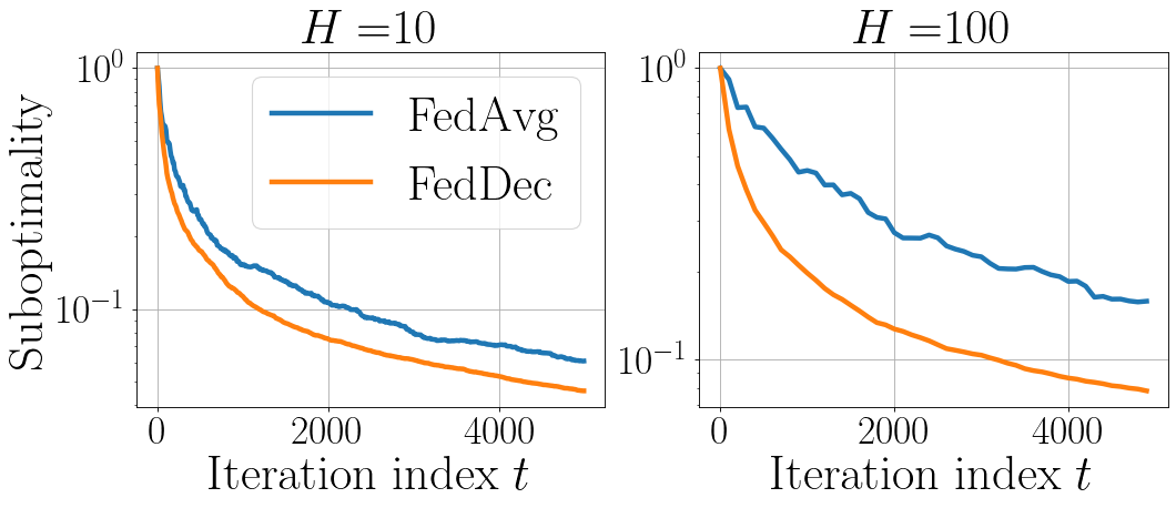
Figure 4: FedDec versus FedAvg for the sparse graph (top) and the dense graph (bottom). When the communication with the server is less frequent (larger $H$), the performance of FedAvg is more degraded than that of FedDec.

Comparing the plots in Fig. 4 vertically (i.e., comparing the two graphs for the same $H$), we confirm that higher connectivity leads to larger gains of FedDec over FedAvg. This can be understood intuitively by noticing that a denser graph facilitates a faster spread of information. Since $|\lambda_{2}|$ correlates with the graph connectivity (see Table 1), in this case it is a good predictor of the convergence speed of FedDec. However, we note that it has been reported that connectivity, as measured by $|\lambda_{2}|$, seems to be predictive of the convergence speed of decentralized algorithms (in terms of number of iterations) only when the nodes have sufficiently different data [28], as is the case in our simulations. When the data is iid among the nodes, the number of effective neighbors seems to be a better predictor [29].

Comparing the plots in Fig. 4 horizontally (i.e., comparing the $H$ for a given graph), we verify that as $H$ increases the convergence speed of FedAvg decreases more than that of FedDec. Therefore, FedDec allows for sparser server communication rounds without significantly sacrificing convergence speed, which is in accordance with Theorem 1.

One may wonder whether in practice $\alpha$ takes values much smaller than $H$ so that the gains of FedDec can actually be observed. Assuming a fixed $W$, this question is equivalent to asking what are typical values for $|\lambda_{2}|^{2}$ (see Fig. 2). Table 1 shows this value for many graphs, where $W$ was constructed using the graph’s Laplacian [26]. We computed these values for geographic graphs with different linking radii $r$ and random graphs with different link probabilities $p$, and in both cases, for different number of nodes. Geographic graphs are good models for wireless networks [30], while random graphs have the small-world property of other kinds of networks, such as the Internet [31]. The values of $r$ and $p$ are such that the networks in the same row and column under each graph type have approximately the same number of edges. The numbers shown are the average over 10 independent realizations, and the values corresponding to the graphs in Fig. 3 are shown in gray. We observe that in all cases $|\lambda_{2}|^{2}<0.9$, which implies $\alpha<9$. Therefore, unless $H$ is particularly small, FedDec is expected to be (potentially, much) faster than FedAvg. In particular, for random graphs, which have low network diameter, $|\lambda_{2}|^{2}$ decreases more abruptly as connectivity grows. This further indicates that for well-connected networks, inter-agent communication can make the first term of $B$ in Theorem 1 become negligible.

Table 1: Values of $|\lambda_{2}|^{2}$ for different graphs.

Geographic graph
Connection radius	$n=10$	$n=20$	$n=40$
$r=0.35$	0.78	0.87	0.83
$r=0.5$	0.7	0.64	0.56
$r=0.65$	0.41	0.33	0.34
Random graph
Link probability	$n=10$	$n=20$	$n=40$
$p=0.3$	0.7	0.62	0.4
$p=0.5$	0.42	0.29	0.17
$p=0.7$	0.25	0.13	0.083

5 Conclusion

We have presented FedDec, an algorithm that exploits inter-agent communication in FL settings by averaging the agents’ parameters with those of their neighbors before each new local SGD update. We proved that this modification reduces the negative impact of local updates on convergence and that the magnitude of this reduction depends on the spectrum of the graph defining the communication network. This further indicates that the effect of local updates and partial device participation can become negligible if the communication network is well-connected.

This insight suggests that there exists a connectivity threshold where the server does not help convergence anymore. Furthermore, we conjecture that for sufficiently dense networks, server communication rounds might even hurt. Future directions include studying this threshold and other trade-offs of peer-to-peer aided FL.

Overall, exploiting inter-agent communication in FL is a promising way to reduce the frequency of server communication rounds without significantly hurting convergence.

Appendix A Useful Properties

This section groups a number of facts used in the proofs.

Fact 1.

For two vectors $u,v\in\mathbb{R}^{d}$ and $\delta>0$ it holds

$$-2{\left\langle{\mathbf{u}},{\mathbf{v}}\right\rangle}\leq\frac{1}{\delta}{\left\lVert{\mathbf{u}}\right\rVert_{2}^{2}}+\delta{\left\lVert{\mathbf{v}}\right\rVert_{2}^{2}}.$$ (10)

This also holds for matrices $u,v\in\mathbb{R}^{m\times n}$ and the Frobenius norm. It can be shown by manipulating the term ${\left\lVert\frac{1}{\delta}{\mathbf{u}}+\delta{\mathbf{v}}\right\rVert}_{2}^{2}\geq 0$.

Fact 2.

For two matrices $A,B\in\mathbb{R}^{m\times n}$ it holds that

$${\left\lVert A+B\right\rVert}_{F}^{2}\leq(1+\alpha^{-1}){\left\lVert A\right\rVert}_{F}^{2}+(1+\alpha){\left\lVert B\right\rVert}_{F}^{2}.$$ (11)

This can be shown using (10).

Fact 3.

For a matrix $A\in\mathbb{R}^{m\times n}$ it can be shown that

$${\left\lVert A{\left(I-{\frac{1}{n}\mathbf{1}\mathbf{1}^{T}}\right)}\right\rVert}_{F}^{2}\leq{\left\lVert A\right\rVert}_{F}^{2}.$$ (12)

Fact 4.

Let $M\in\mathbb{R}^{n\times n}$ be a symmetric matrix satisfying $\mathbf{1}^{T}M=\mathbf{1}$ and having eigenvalues $1=\lambda_{1}>{\left|\lambda_{2}\right|}\geq\ldots\geq{\left|\lambda_{n}\right|}$. Then, for a vector ${\mathbf{x}}\in\mathbb{R}^{n}$ with the average of its entries denoted $x_{\text{avg}}=\mathbf{1}^{T}{\mathbf{x}}$, it holds

$$({\mathbf{x}}-x_{\text{avg}}\mathbf{1})^{T}M({\mathbf{x}}-x_{\text{avg}}\mathbf{1})\leq|\lambda_{2}|\,{\left\lVert{\mathbf{x}}-x_{\text{avg}}\mathbf{1}\right\rVert}_{2}^{2}.$$ (13)

This is a consequence of the spectral theorem and the fact that $({\mathbf{x}}-x_{\text{avg}}\mathbf{1})\perp\text{span}\{\mathbf{1}\}$.

Appendix B Proofs of Lemmas

Proof of Lemma 2.

It holds that

$$\mathbb{E}{{\left\lVert{\overline{{\mathbf{x}}}}^{t+1}-{\mathbf{z}^{*}}\right\rVert_{2}^{2}}} =\mathbb{E}{{\left\lVert{\overline{{\mathbf{z}}}}^{t}-\frac{\eta_{t}}{n}{\sum_{i=1}^{n}}\nabla F_{i}({\mathbf{z}}_{i}^{t},\xi_{i}^{t})-{\mathbf{z}^{*}}\right\rVert}_{2}^{2}}$$

$$=\mathbb{E}{\left\lVert{\overline{{\mathbf{z}}}}^{t}-{\mathbf{z}^{*}}-\frac{\eta_{t}}{n}{\sum_{i=1}^{n}}\nabla F_{i}({\mathbf{z}}_{i}^{t})\right\rVert_{2}^{2}}+\eta_{t}^{2}\;\mathbb{E}{\left\lVert\frac{1}{n}{\sum_{i=1}^{n}}\nabla F_{i}({\mathbf{z}}_{i}^{t})-\frac{1}{n}{\sum_{i=1}^{n}}\nabla F_{i}({\mathbf{z}}_{i}^{t},\xi_{i}^{j_{t}})\right\rVert}_{2}^{2}$$

$$\qquad+2\;\mathbb{E}\biggl{\langle}{\overline{{\mathbf{z}}}}^{t}-{\mathbf{z}^{*}}-\frac{\eta_{t}}{n}{\sum_{i=1}^{n}}\nabla F_{i}({\mathbf{z}}_{i}^{t}),\frac{\eta_{t}}{n}{\sum_{i=1}^{n}}\nabla F_{i}({\mathbf{z}}_{i}^{t})-\frac{\eta_{t}}{n}{\sum_{i=1}^{n}}\nabla F_{i}({\mathbf{z}}_{i}^{t},\xi_{i}^{j_{t}})\biggr{\rangle}$$ (14)

where in the first equality we used that

$${\overline{{\mathbf{x}}}}^{t+1}=\frac{1}{n}{\sum_{i=1}^{n}}{\mathbf{x}}_{i}^{t+1}=\frac{1}{n}{\sum_{i=1}^{n}}\sum_{j=1}^{n}W_{ij}{\mathbf{x}}_{i}^{t+\frac{1}{2}}=\frac{1}{n}{\sum_{i=1}^{n}}{\mathbf{x}}_{i}^{t+\frac{1}{2}}\sum_{j=1}^{n}W_{ij}={\overline{{\mathbf{x}}}}^{t+\frac{1}{2}}={\overline{{\mathbf{z}}}}^{t}-\frac{\eta_{t}}{n}{\sum_{i=1}^{n}}\nabla F_{i}({\mathbf{z}}_{i}^{t},\xi_{i}^{t})$$

and in the second equality we added and subtracted $\frac{\eta_{t}}{n}{\sum_{i=1}^{n}}\nabla F_{i}({\mathbf{x}}_{i}^{t})$ inside the norm.

Note that the last term in (14) is zero, since $\mathbb{E}_{\xi_{i}^{t}}[\nabla F_{i}({\mathbf{z}}_{i}^{t},\xi_{i}^{t})]=\nabla F_{i}({\mathbf{z}}_{i}^{t})$, and the second term is bounded by $\eta_{t}^{2}\frac{{\overline{\sigma}}^{2}}{n}$ (eq. (6)). The first term in (14) can be written as (we will apply the expectation directly to the end result)

$${\left\lVert{\overline{{\mathbf{z}}}}^{t}-{\mathbf{z}^{*}}-\frac{\eta_{t}}{n}{\sum_{i=1}^{n}}\nabla F_{i}({\mathbf{z}}_{i}^{t})\right\rVert_{2}^{2}}={\left\lVert{\overline{{\mathbf{z}}}}^{t}-{\mathbf{z}^{*}}\right\rVert_{2}^{2}}+\eta_{t}^{2}\underbrace{{\left\lVert\frac{1}{n}{\sum_{i=1}^{n}}\nabla F_{i}({\mathbf{z}}_{i}^{t})\right\rVert_{2}^{2}}}_{(A)}\underbrace{-2\eta_{t}{\left\langle{\overline{{\mathbf{z}}}}^{t}-{\mathbf{z}^{*}},\frac{1}{n}{\sum_{i=1}^{n}}\nabla F_{i}({\mathbf{z}}_{i}^{t})\right\rangle}}_{(B)}.$$ (15)

We can bound term $(A)$ with

$${\left\lVert\frac{1}{n}{\sum_{i=1}^{n}}\nabla F_{i}({\mathbf{z}}_{i}^{t})\right\rVert_{2}^{2}} \leq\frac{1}{n}{\sum_{i=1}^{n}}{\left\lVert\nabla F_{i}({\mathbf{z}}_{i}^{t})\right\rVert_{2}^{2}}$$

$$=\frac{1}{n}{\sum_{i=1}^{n}}{\left\lVert\nabla F_{i}({\mathbf{z}}_{i}^{t})-\nabla F_{i}({\mathbf{z}}_{i}^{*})\right\rVert_{2}^{2}}$$

$$\stackrel{{\scriptstyle\eqref{eq:smooth_df2_leq_ffs}}}{{\leq}}\frac{1}{n}{\sum_{i=1}^{n}}2L(F_{i}({\mathbf{z}}_{i}^{t})-F_{i}({\mathbf{z}}_{i}^{*})).$$ (16)

On the other hand, term $(B)$ can be bounded as

$$-2\eta_{t}{\left\langle{\overline{{\mathbf{z}}}}^{t}-{\mathbf{z}^{*}},\frac{1}{n}{\sum_{i=1}^{n}}\nabla F_{i}({\mathbf{z}}_{i}^{t})\right\rangle} =\frac{-2\eta_{t}}{n}{\sum_{i=1}^{n}}{\left\langle{\overline{{\mathbf{z}}}}^{t}-{\mathbf{z}}_{i}^{t}+{\mathbf{z}}_{i}^{t}-{\mathbf{z}^{*}},\nabla F_{i}({\mathbf{z}}_{i}^{t})\right\rangle}$$

$$=\frac{-2\eta_{t}}{n}{\sum_{i=1}^{n}}{\left\langle{\overline{{\mathbf{z}}}}^{t}-{\mathbf{z}}_{i}^{t},\nabla F_{i}({\mathbf{z}}_{i}^{t})\right\rangle}-\frac{2\eta_{t}}{n}{\sum_{i=1}^{n}}{\left\langle{\mathbf{z}}_{i}^{t}-{\mathbf{z}^{*}},\nabla F_{i}({\mathbf{z}}_{i}^{t})\right\rangle}$$

$$\stackrel{{\scriptstyle\eqref{eq:CS_AM-GM},\eqref{eq:strong_conv}}}{{\leq}}\frac{\eta_{t}}{n}{\sum_{i=1}^{n}}{\left(\frac{1}{\eta_{t}}{\left\lVert{\overline{{\mathbf{z}}}}^{t}-{\mathbf{z}}_{i}^{t}\right\rVert}_{2}^{2}+\eta_{t}{\left\lVert\nabla F_{i}({\mathbf{z}}_{i}^{t})\right\rVert}_{2}^{2}\right)}$$

$$\qquad-\frac{2\eta_{t}}{n}{\sum_{i=1}^{n}}{\left((F_{i}({\mathbf{z}}_{i}^{t})-F_{i}({\mathbf{z}^{*}}))+\frac{\mu}{2}{\left\lVert{\mathbf{z}}_{i}^{t}-{\mathbf{z}^{*}}\right\rVert}_{2}^{2}\right)}.$$

where we applied (10) with the choice $\delta=\eta_{t}$.

Replacing the bounds on $(A)$ and $(B)$ in (14) gives

$${\left\lVert{\overline{{\mathbf{z}}}}^{t}-{\mathbf{z}^{*}}-\frac{\eta_{t}}{n}{\sum_{i=1}^{n}}\nabla F_{i}({\mathbf{z}}_{i}^{t})\right\rVert}_{2}^{2} \leq{\left\lVert{\overline{{\mathbf{z}}}}^{t}-{\mathbf{z}^{*}}\right\rVert_{2}^{2}}+\frac{\eta_{t}^{2}}{n}2L{\sum_{i=1}^{n}}(F_{i}({\mathbf{z}}_{i}^{t})-F_{i}({\mathbf{z}}_{i}^{*}))+\frac{\eta_{t}}{n}{\sum_{i=1}^{n}}{\left(\frac{1}{\eta_{t}}{\left\lVert{\overline{{\mathbf{z}}}}^{t}-{\mathbf{z}}_{i}^{t}\right\rVert}_{2}^{2}+\eta_{t}{\left\lVert\nabla F_{i}({\mathbf{z}}_{i}^{t})\right\rVert}_{2}^{2}\right)}$$

$$\qquad-\frac{2\eta_{t}}{n}{\sum_{i=1}^{n}}{\left((F_{i}({\mathbf{z}}_{i}^{t})-F_{i}({\mathbf{z}^{*}}))+\frac{\mu}{2}{\left\lVert{\mathbf{z}}_{i}^{t}-{\mathbf{z}^{*}}\right\rVert}_{2}^{2}\right)}$$

$$\stackrel{{\scriptstyle\eqref{eq:bound_norm_grad_Fi}}}{{\leq}}(1-\mu\eta_{t}){\left\lVert{\overline{{\mathbf{z}}}}^{t}-{\mathbf{z}^{*}}\right\rVert}_{2}^{2}+\frac{1}{n}{\sum_{i=1}^{n}}{\left\lVert{\overline{{\mathbf{z}}}}^{t}-{\mathbf{z}}_{i}^{t}\right\rVert}_{2}^{2}$$

$$\qquad+\underbrace{\eta_{t}^{2}\frac{4L}{n}{\sum_{i=1}^{n}}(F_{i}({\mathbf{z}}_{i}^{t})-F_{i}({\mathbf{z}}_{i}^{*}))-\frac{2\eta_{t}}{n}{\sum_{i=1}^{n}}(F_{i}({\mathbf{z}}_{i}^{t})-F_{i}({\mathbf{z}^{*}}))}_{(C)}$$

where we used

$$-\frac{\eta_{t}\mu}{n}{\sum_{i=1}^{n}}{\left\lVert{\mathbf{z}}_{i}^{t}-{\mathbf{z}^{*}}\right\rVert}_{2}^{2}\leq-\eta_{t}\mu{\left\lVert\frac{1}{n}{\sum_{i=1}^{n}}({\mathbf{z}}_{i}^{t}-{\mathbf{z}^{*}})\right\rVert}_{2}^{2}\\ =-\eta_{t}\mu{\left\lVert{\overline{{\mathbf{z}}}}^{t}-{\mathbf{z}^{*}}\right\rVert}_{2}^{2}.$$

Term $(C)$ was bounded in the proof of Lemma 1 of [16], where for $\eta_{t}\leq\frac{1}{4L}$ and $\Gamma=\frac{1}{n}{\sum_{i=1}^{n}}(F_{i}({\mathbf{z}^{*}})-F_{i}({\mathbf{z}}_{i}^{*}))$ they obtained

$$(C)\leq\frac{1}{n}{\sum_{i=1}^{n}}{\left\lVert{\mathbf{z}}_{i}^{t}-{\overline{{\mathbf{z}}}}^{t}\right\rVert_{2}^{2}}+6L\eta_{t}^{2}\Gamma.$$

Replacing these bounds in (14) gives the lemma. ∎

Proof of Lemma 3.

We define

$$Z^{t}={\left[{\mathbf{z}}_{1}^{t}\cdots{\mathbf{z}}_{n}^{t}\right]}\in\mathbb{R}^{d\times n}$$

$$\overline{Z}^{t}=Z^{t}{\frac{1}{n}\mathbf{1}\mathbf{1}^{T}}={\left[{\overline{{\mathbf{z}}}}^{t}\cdots{\overline{{\mathbf{z}}}}^{t}\right]}\in\mathbb{R}^{d\times n}$$

$$\partial F(Z^{t},\xi^{t})={\left[\nabla F_{1}({\mathbf{z}}_{1}^{t},\xi_{1}^{t})\cdots\nabla F_{n}({\mathbf{z}}_{n}^{t},\xi_{n}^{t})\right]}\in\mathbb{R}^{d\times n}$$

and $X^{t},\overline{X}^{t}$ analogously. Note that with these definitions, ${\sum_{i=1}^{n}}{\left\lVert{\mathbf{z}}_{i}^{t}-{\overline{{\mathbf{z}}}}^{t}\right\rVert}_{2}^{2}={\left\lVert Z^{t}-\overline{Z}^{t}\right\rVert}_{F}^{2}$.

We denote $t_{b}\in\mathcal{H}$ the last time the central server broadcasted the sample average to all nodes so that ${\mathbf{z}}_{i}^{t_{b}}={\mathbf{z}}^{t_{b}}\;\forall i\in[n]$, and define $h:=t-t_{b}\leq(H-1)$. Note that if $t=t_{b}$ then ${\sum_{i=1}^{n}}{\left\lVert{\mathbf{z}}_{i}^{t}-{\overline{{\mathbf{z}}}}\right\rVert}_{2}^{2}=0$. Therefore, below we assume $h\geq 1$. We have that

$$\mathbb{E}{\left\lVert Z^{t}-\overline{Z}^{t}\right\rVert}_{F}^{2}\stackrel{{\scriptstyle t\notin\mathcal{H}}}{{=}} \mathbb{E}{\left\lVert X^{t}-\overline{X}^{t}\right\rVert}_{F}^{2}=\mathbb{E}\Big{\|}\underbrace{(X^{t-\frac{1}{2}}-\overline{X}^{t-\frac{1}{2}})}_{Y}W^{t-1}\Big{\|}_{F}^{2}$$

$$=\mathbb{E}\sum_{i=1}^{d}{\left\lVert Y_{[i,:]}W^{t-1}\right\rVert}_{2}^{2}$$

$$=\mathbb{E}\sum_{i=1}^{d}Y_{[i,:]}\mathbb{E}_{W}{\left[WW^{T}\right]}[Y_{[i,:]}]^{T}$$

$$\stackrel{{\scriptstyle\eqref{eq:bound_lambda_2}}}{{\leq}}\mathbb{E}\sum_{i=1}^{d}Y_{[i,:]}\underbrace{{\left|\lambda_{2}{\left(\mathbb{E}_{W}{\left[WW^{T}\right]}\right)}\right|}}_{|\widehat{\lambda}_{2}|}\,[Y_{[i,:]}]^{T}$$

$$=|\widehat{\lambda}_{2}|\;\mathbb{E}{\left\lVert X^{t-\frac{1}{2}}-\overline{X}^{t-\frac{1}{2}}\right\rVert}_{F}^{2}$$

$$=|\widehat{\lambda}_{2}|\;\mathbb{E}\Big{\|}Z^{t-1}-\overline{Z}^{t-1}-\eta_{t-1}\partial F(Z^{t-1},\xi^{t-1})(I-{\frac{1}{n}\mathbf{1}\mathbf{1}^{T}})\Big{\|}_{F}^{2}$$

$$\stackrel{{\scriptstyle\eqref{eq:bound_frob_A+B_alphas}}}{{\leq}}|\widehat{\lambda}_{2}|{\left(1+\frac{1}{\alpha}\right)}\mathbb{E}{\left\lVert Z^{t-1}-\overline{Z}^{t-1}\right\rVert}_{F}^{2}+|\widehat{\lambda}_{2}|(1+\alpha)\eta_{t-1}^{2}\mathbb{E}{\left\lVert\partial F(Z^{t-1},\xi^{t-1})(I-{\frac{1}{n}\mathbf{1}\mathbf{1}^{T}})\right\rVert}_{F}^{2}$$

$$\stackrel{{\scriptstyle\eqref{eq:bound_frob_A-n11}}}{{\leq}}|\widehat{\lambda}_{2}|{\left(1+\frac{1}{\alpha}\right)}\mathbb{E}{\left\lVert Z^{t-1}-\overline{Z}^{t-1}\right\rVert}_{F}^{2}+|\widehat{\lambda}_{2}|\ (1+\alpha)\eta_{t-1}^{2}\mathbb{E}{\left\lVert\partial F(Z^{t-1},\xi^{t-1})\right\rVert}_{F}^{2}$$

$$=|\widehat{\lambda}_{2}|{\left(1+\frac{1}{\alpha}\right)}\mathbb{E}{\left\lVert Z^{t-1}-\overline{Z}^{t-1}\right\rVert}_{F}^{2}{+}\ |\widehat{\lambda}_{2}|(1+\alpha)\eta_{t-1}^{2}nG^{2},$$

where in the second line we used that $\mathbf{1}^{T}W^{t}=\mathbf{1}^{T}$, and in the fourth line, that the matrices $W^{t}$ are identically distributed independently of the time $t$. We also used $Y_{[i,:]}$ to indicate the $i$-th row of matrix $Y$.

We can now apply the inequality recursively to get

$$\mathbb{E}{\left\lVert Z^{t}-\overline{Z}^{t}\right\rVert}_{F}^{2} \leq{\left(1+\frac{1}{\alpha}\right)}|\widehat{\lambda}_{2}|\;\mathbb{E}{\left\lVert Z^{t-1}-\overline{Z}^{t-1}\right\rVert}_{F}^{2}+(1+\alpha)|\widehat{\lambda}_{2}|\;\eta_{t-1}^{2}nG^{2}$$

$$\leq{\left(1+\frac{1}{\alpha}\right)}|\widehat{\lambda}_{2}|\;\Bigg{[}{\left(1+\frac{1}{\alpha}\right)}|\widehat{\lambda}_{2}|\;\mathbb{E}{\left\lVert Z^{t-2}-\overline{Z}^{t-2}\right\rVert}_{F}^{2}+(1+\alpha)|\widehat{\lambda}_{2}|\;\eta_{t-2}^{2}nG^{2}\Bigg{]}+(1+\alpha)|\widehat{\lambda}_{2}|\;\eta_{t-1}^{2}nG^{2}$$

$$={\left[{\left(1+\frac{1}{\alpha}\right)}|\widehat{\lambda}_{2}|\;\right]}^{2}\mathbb{E}{\left\lVert Z^{t-2}-\overline{Z}^{t-2}\right\rVert}_{F}^{2}+(1+\alpha)|\widehat{\lambda}_{2}|\;nG^{2}\sum_{i=1}^{2}{\left[{\left(1+\frac{1}{\alpha}\right)}|\widehat{\lambda}_{2}|\;\right]}^{i-1}\eta_{t-i}^{2}$$

$$\leq{\left[{\left(1+\frac{1}{\alpha}\right)}|\widehat{\lambda}_{2}|\;\right]}^{h}\mathbb{E}{\left\lVert Z^{t_{b}}-\overline{Z}^{t_{b}}\right\rVert}_{F}^{2}+(1+\alpha)|\widehat{\lambda}_{2}|\;nG^{2}\sum_{i=1}^{h}{\left[{\left(1+\frac{1}{\alpha}\right)}|\widehat{\lambda}_{2}|\;\right]}^{i-1}\eta_{t-i}^{2}.$$

We note that the first term is zero, since at broadcasting time $Z^{t_{b}}=\overline{Z}^{t_{b}}$. We now set $\alpha=\frac{|\widehat{\lambda}_{2}|}{1-|\widehat{\lambda}_{2}|}$ so that the expression between square brackets takes value 1. Therefore,

$$\mathbb{E}{\left\lVert Z^{t}-\overline{Z}^{t}\right\rVert}_{F}^{2}\leq\alpha nG^{2}H\eta_{t_{b}}^{2}\leq\alpha nG^{2}H4\eta_{t}^{2}$$

where we have used that for the choice of $\alpha$ given above it holds $(1+\alpha)|\widehat{\lambda}_{2}|\;=\alpha$, and that the stepsizes $\eta_{t}$ are monotonically decreasing and satisfy $\eta_{t}\leq 2\eta_{t+H}$. ∎

Note that in the result above we could have used $(H-1)$ instead of $H$. However, since this bound is used again in the proof of Lemma 4 for $h=H$, we loosen it slightly here to be able to apply it directly in the next proof.

Proof of Lemma 4.

For $t\in\mathcal{H}$ we have that

$$\mathbb{E}{\left\lVert{\overline{{\mathbf{z}}}}^{t}-{\overline{{\mathbf{x}}}}^{t}\right\rVert_{2}^{2}}=\mathbb{E}{\left\lVert\frac{1}{K}\sum_{\ell=1}^{K}{\mathbf{x}}_{j_{\ell}}^{t}-{\overline{{\mathbf{x}}}}^{t}\right\rVert_{2}^{2}}\\ =\frac{1}{K^{2}}\sum_{\ell=1}^{K}\mathbb{E}{\left[{\mathbb{E}_{\mathcal{S}_{t}}}{\left\lVert{\mathbf{x}}_{j_{\ell}}^{t}-{\overline{{\mathbf{x}}}}^{t}\right\rVert_{2}^{2}}\right]}=\frac{1}{Kn}{\sum_{i=1}^{n}}\mathbb{E}{\left\lVert{\mathbf{x}}_{i}^{t}-{\overline{{\mathbf{x}}}}^{t}\right\rVert_{2}^{2}}$$

where we used that for independent $X_{i}$, $\text{Var}(\sum_{i}X_{i})=\sum_{i}\text{Var}(X_{i})$, and that for a random variable $X\in\Omega$ with a discrete probability density function $X\sim f_{X}$ and a function $g:\Omega\rightarrow\mathbb{R}$ it holds $\mathbb{E}[g(X)]=\sum_{x}g(x)f_{X}(x)$.

Since ${\sum_{i=1}^{n}}{\left\lVert{\mathbf{x}}_{i}^{t}-{\overline{{\mathbf{x}}}}^{t}\right\rVert_{2}^{2}}=\big{\|}X^{t}-\overline{X}^{t}\big{\|}_{F}^{2}$ we can repeat the procedure done in Lemma 3 to bound this term. ∎

References

• [1] B. McMahan, E. Moore, D. Ramage, S. Hampson, and B. A. y Arcas, “Communication-efficient learning of deep networks from decentralized data,” in Artificial intelligence and statistics, pp. 1273–1282, PMLR, 2017.
• [2] S. P. Karimireddy, S. Kale, M. Mohri, S. Reddi, S. Stich, and A. T. Suresh, “Scaffold: Stochastic controlled averaging for federated learning,” in International Conference on Machine Learning, pp. 5132–5143, PMLR, 2020.
• [3] T. Li, A. K. Sahu, M. Zaheer, M. Sanjabi, A. Talwalkar, and V. Smith, “Federated optimization in heterogeneous networks,” Proceedings of Machine learning and systems, vol. 2, pp. 429–450, 2020.
• [4] Z. Qu, K. Lin, Z. Li, and J. Zhou, “Federated learning’s blessing: Fedavg has linear speedup,” in ICLR 2021-Workshop on Distributed and Private Machine Learning (DPML), 2021.
• [5] L. Xiao, A. W. Yu, Q. Lin, and W. Chen, “DSCOVR: Randomized primal-dual block coordinate algorithms for asynchronous distributed optimization,” The Journal of Machine Learning Research, vol. 20, no. 1, pp. 1634–1691, 2019.
• [6] B. Recht, C. Re, S. Wright, and F. Niu, “Hogwild!: A lock-free approach to parallelizing stochastic gradient descent,” Advances in neural information processing systems, vol. 24, 2011.
• [7] J. Liu, S. Wright, C. Ré, V. Bittorf, and S. Sridhar, “An asynchronous parallel stochastic coordinate descent algorithm,” in International Conference on Machine Learning, pp. 469–477, PMLR, 2014.
• [8] V. Smith, S. Forte, M. Chenxin, M. Takác, M. I. Jordan, and M. Jaggi, “CoCoA: A general framework for communication-efficient distributed optimization,” Journal of Machine Learning Research, vol. 18, p. 230, 2018.
• [9] A. Nedic and A. Ozdaglar, “Distributed subgradient methods for multi-agent optimization,” IEEE Transactions on Automatic Control, vol. 54, no. 1, pp. 48–61, 2009.
• [10] W. Shi, Q. Ling, G. Wu, and W. Yin, “Extra: An exact first-order algorithm for decentralized consensus optimization,” SIAM Journal on Optimization, vol. 25, no. 2, pp. 944–966, 2015.
• [11] J. C. Duchi, A. Agarwal, and M. J. Wainwright, “Dual averaging for distributed optimization: Convergence analysis and network scaling,” IEEE Transactions on Automatic control, vol. 57, no. 3, pp. 592–606, 2011.
• [12] K. Scaman, F. Bach, S. Bubeck, Y. T. Lee, and L. Massoulié, “Optimal algorithms for smooth and strongly convex distributed optimization in networks,” in international conference on machine learning, pp. 3027–3036, PMLR, 2017.
• [13] X. Lian, C. Zhang, H. Zhang, C.-J. Hsieh, W. Zhang, and J. Liu, “Can decentralized algorithms outperform centralized algorithms? a case study for decentralized parallel stochastic gradient descent,” Advances in Neural Information Processing Systems, vol. 30, 2017.
• [14] A. Koloskova, S. Stich, and M. Jaggi, “Decentralized stochastic optimization and gossip algorithms with compressed communication,” in International Conference on Machine Learning, pp. 3478–3487, PMLR, 2019.
• [15] C. A. Uribe, S. Lee, A. Gasnikov, and A. Nedić, “A dual approach for optimal algorithms in distributed optimization over networks,” in 2020 Information Theory and Applications Workshop (ITA), pp. 1–37, IEEE, 2020.
• [16] X. Li, K. Huang, W. Yang, S. Wang, and Z. Zhang, “On the convergence of FedAvg on non-iid data,” in International Conference on Learning Representations, 2020.
• [17] J. Zhang, C. De Sa, I. Mitliagkas, and C. Ré, “Parallel SGD: When does averaging help?,” arXiv preprint arXiv:1606.07365, 2016.
• [18] H. Hellaoui, O. Bekkouche, M. Bagaa, and T. Taleb, “Aerial control system for spectrum efficiency in uav-to-cellular communications,” IEEE Communications Magazine, vol. 56, no. 10, pp. 108–113, 2018.
• [19] A. Asadi, Q. Wang, and V. Mancuso, “A survey on device-to-device communication in cellular networks,” IEEE Communications Surveys & Tutorials, vol. 16, no. 4, pp. 1801–1819, 2014.
• [20] S. U. Stich, “Local SGD converges fast and communicates little,” in ICLR 2019-International Conference on Learning Representations, no. CONF, 2019.
• [21] M. Yemini, R. Saha, E. Ozfatura, D. Gündüz, and A. J. Goldsmith, “Semi-decentralized federated learning with collaborative relaying,” in 2022 IEEE International Symposium on Information Theory (ISIT), pp. 1471–1476, IEEE, 2022.
• [22] F. P.-C. Lin, S. Hosseinalipour, S. S. Azam, C. G. Brinton, and N. Michelusi, “Semi-decentralized federated learning with cooperative D2D local model aggregations,” IEEE Journal on Selected Areas in Communications, vol. 39, no. 12, pp. 3851–3869, 2021.
• [23] L. Chou, Z. Liu, Z. Wang, and A. Shrivastava, “Efficient and less centralized federated learning,” in Machine Learning and Knowledge Discovery in Databases. Research Track: European Conference, ECML PKDD 2021, Bilbao, Spain, September 13–17, 2021, Proceedings, Part I 21, pp. 772–787, Springer, 2021.
• [24] S. Hosseinalipour, S. S. Azam, C. G. Brinton, N. Michelusi, V. Aggarwal, D. J. Love, and H. Dai, “Multi-stage hybrid federated learning over large-scale d2d-enabled fog networks,” IEEE/ACM Transactions on Networking, vol. 30, no. 4, pp. 1569–1584, 2022.
• [25] A. Koloskova, N. Loizou, S. Boreiri, M. Jaggi, and S. Stich, “A unified theory of decentralized SGD with changing topology and local updates,” in International Conference on Machine Learning, pp. 5381–5393, PMLR, 2020.
• [26] L. Xiao and S. Boyd, “Fast linear iterations for distributed averaging,” Systems & Control Letters, vol. 53, no. 1, pp. 65–78, 2004.
• [27] S. Boyd, A. Ghosh, B. Prabhakar, and D. Shah, “Randomized gossip algorithms,” IEEE transactions on information theory, vol. 52, no. 6, pp. 2508–2530, 2006.
• [28] G. Neglia, C. Xu, D. Towsley, and G. Calbi, “Decentralized gradient methods: does topology matter?,” in International Conference on Artificial Intelligence and Statistics, pp. 2348–2358, PMLR, 2020.
• [29] T. Vogels, H. Hendrikx, and M. Jaggi, “Beyond spectral gap: The role of the topology in decentralized learning,” arXiv preprint arXiv:2206.03093, 2022.
• [30] M. Barthélemy, “Spatial networks,” Physics reports, vol. 499, no. 1-3, pp. 1–101, 2011.
• [31] M. E. Newman, “The structure and function of complex networks,” SIAM review, vol. 45, no. 2, pp. 167–256, 2003.