Information-Theoretic Limits of Bistatic Integrated Sensing and Communication

Abstract

The bistatic integrated sensing and communication (ISAC) system model avoids the strong self-interference in a monostatic ISAC system by employing a pair of physically separated sensing transceiver and maintaining the merit of co-designing radar sensing and communications on shared spectrum and hardware. Inspired by the appealing benefits of bistatic radar, we study bistatic ISAC, where a transmitter sends a message to a communication receiver and a sensing receiver at another location carries out a decoding-and-estimation (DnE) operation to obtain the state of the communication receiver. In this paper, both communication and sensing channels are modelled as state-dependent memoryless channels with independent and identically distributed time-varying state sequences. We consider a rate of reliable communication for the message at the communication receiver as communication metric. The objective of this model is to characterize the capacity-distortion region, i.e., the set of all the achievable rate while simultaneously allowing the sensing receiver to sense the state sequence with a given distortion threshold. In terms of the decoding degree on this message at the sensing receiver, we propose three achievable DnE strategies, the blind estimation, the partial-decoding-based estimation, and the full-decoding-based estimation, respectively. Based on the three strategies, we derive the three achievable rate-distortion regions. In addition, under the constraint of the degraded broadcast channel, i.e., the communication receiver is statistically stronger than the sensing receiver, and the partial-decoding-based estimation, we characterize the capacity region. Examples in both non-degraded and degraded cases are provided to compare the achievable rate-distortion regions under three DnE strategies and demonstrate the advantages of ISAC over independent communication and sensing.

I Introduction

Integrated sensing and communication (ISAC) has become a key technology for beyond 5G and 6G since many practical scenarios place high demands on sensing and communication [1, 2]. In future vehicular networks, self-driving technologies not only require a high data rate for obtaining important information such as media messages, ultra-high-resolution maps, and real-time traffic information, but also need sensing functionality to provide robust and high-resolution obstacle detection [3]. Besides, with the wide application of emerging wireless technologies, e.g., millimeter waves [4, 5] and massive multiple-input multiple-output (MIMO) [6, 7, 8, 9], the communication signals in future wireless systems tend to be of high resolution in both time and angle domains, which has the potential to be used for realizing high-precision sensing. Therefore, it is expected to integrate sensing and communication functionalities into one platform so that they can share the same frequency bands and hardware to improve spectral efficiency and to reduce hardware cost.

Sensing and communication process information in different ways. Sensing gathers and extracts information from noisy observations by using deterministic signals (i.e., test signals), while communication focuses on sending information through random signals under some distribution and then recovering information from noisy received signals. The ultimate goal of ISAC is to unify these two functionalities and to find the performance tradeoff between them. Therefore, by integrating sensing and communication into a unified system and sharing system resources, ISAC improves spectrum and energy efficiency while reducing hardware and signaling costs. Besides, ISAC is also pursuing mutual benefits through communication-assisted sensing and sensing-assisted communication [10].

Sensing, mainly referring to radar in this paper, has a long research history [11, 12, 13]. According to the distribution of transceiver, radar systems can be classified as monostatic, bistatic, and multistatic. In particular, a radar with physically-colocated transmit and receiver arrays is called a monostatic radar, and in many cases the same antenna array is used for both transmitting and receiving. A radar with physically-separated transmitter and receiver arrays is called a bistatic radar. If multiple separated receivers are employed with one transmitter, the radar system is called multistatic [11]. Although the bistatic radar system is generally more complicated to implement than the monostatic system [12], the potential of bistatic measurements to detect low-observable targets has stimulated continued research. For example, a target that is designed to minimize backscatter by reflecting radar energy in other directions is difficult to be detected by monostatic radar, while it may be easily detected by bistatic radar [13]. In addition, in the monostatic radar system, the interference from the transmit array to the receiver array cannot be ignored, while the self-interference is negligible in the bistatic radar system as the transmit and receiver arrays are far apart. Inspired by the appealing benefits of bistatic radar, we study bistatic ISAC in this paper.

ISAC has attracted a lot of attention in the field of both radar and wireless communications [14, 15, 16, 17, 18, 19, 20]. Existing studies are mainly limited to system design [14, 15], and to its interplay with other technologies, such as orthogonal time-frequency-space (OTFS) [16], millimeter-wave [17], massive MIMO [18], and reconfigurable intelligent surfaces [19, 20]. However, the investigation of the information-theoretic limits of ISAC is still in its infancy and many important issues of ISAC are still open, such as a unified theoretical framework and the optimal ISAC strategies and corresponding algorithms. In particular, describing the fundamental limits of ISAC, including the sensing limit, channel capacity, and capacity-distortion tradeoff, is of great significance for the breakthrough of the ISAC technology. This not only provides a theoretical limit for ISAC to measure its performance gain or gap with respect to existing techniques, but also provides useful guidelines and insights for the design and analysis of practical ISAC systems. Recent works have been devoted to studying the fundamental limits of ISAC [21, 22, 23, 24, 25, 26]. The authors in [21] and [22] characterized the optimal tradeoffs between the communication rate and the state estimation error at the receiver (i.e., the receiver wants to receive pure communication information and estimate some channel state information simultaneously) when the transmitter causally knows or does not know the state, respectively. The optimal tradeoff between the communication rate and the state estimation distortion at the receiver for Gaussian multiple access channel (GMAC) with additive states, was investigated in [23]. Furthermore, the authors in [24] and [25] systematically studied the capacity-distortion tradeoff of ISAC in the monostatic system by exploiting the backscattered echoes at the transmitter for sensing instead of estimating the state at the receiver. The authors in [26] studied the deterministic and random tradeoff between sensing and communication with vector Gaussian channel models, where the sent information is assumed to be known to the sensing receiver.

Contributions

Figure 1: The bistatic ISAC system model.

In this paper, we formulate a bistatic ISAC model in a state-dependent discrete memoryless channel with independent and identically distributed (i.i.d.) state sequences. As illustrated in Fig. 1, the considered bistatic ISAC system consists of an ISAC transmitter, a communication receiver, and a sensing receiver. The ISAC transmitter sends a message to the communication receiver that wants to fully recover the message. The sensing receiver at another location performs decoding-and-estimation (DnE) to acquire the state of the communication receiver. Because of the broadcast channel, the sensing receiver can also decode parts of the message required by the communication receiver. By using rate splitting, the message could be divided into two parts, the first of which is the common part decoded by both the sensing and communication receivers and the second of which is the refinement part uniquely decoded by the communication receiver. The sensing performance is measured by the distortion function between the target and estimation. Thus the new problem is essentially a two-receiver state-dependent memoryless broadcast channel with degraded message sets (SDMBC-DMS). The objective of the model is to characterize the capacity-distortion region, which is the set of all achievable rate pairs given a distortion limitation. Note that the information theoretic bistatic ISAC problem was originally considered in [27], where the radar (sensing) receiver is located near the transmitter and estimates or detects the state based on the transmitter’s channel inputs and the backscattered signals. Different from the above model, in the considered bistatic ISAC model, the sensing receiver is unaware of the transmitter’s channel inputs and it needs to decode part of the message from the transmitter to estimate the state. Compared to the monostatic ISAC scenario in [25] where the sensing receiver exactly knows the sent message $X$, the main difference of the considered bistatic ISAC model is that the sensing receiver is an individual entity that does not have $X$ as the side information in advance. Different from [25], the main novelty of this work is to propose three DnE strategies depending on the number of bits in $X$ the sensing receiver should decode in prior to estimating the state, and then to provide further analysis of the capacity-distortion region under these three strategies.

In addition to the new problem formulation, our main contributions are as follows.

• In terms of the decoding degree on this message at the sensing receiver (i.e., the rate of the common part), we propose three DnE strategies, i.e., the blind estimation, the partial-decoding-based estimation, and the full-decoding-based estimation.

• We apply the partial-decoding-based estimation strategy to get the rate-distortion region. We further show that this strategy can attain the exact capacity-distortion region under the constraint of the degraded broadcast channel, i.e., the communication receiver is statistically stronger than the sensing receiver. Furthermore, we obtain the rate-distortion region under the blind estimation strategy and the capacity-distortion region under the full-decoding-based estimation strategy.

• Examples in both non-degraded broadcast channel and degraded broadcast channel are provided to numerically compare the rate-distortion regions of the three DnE strategies and to demonstrate the advantages of bistatic ISAC over two benchmark time-sharing schemes of communication and sensing.

In order to express the conclusions of the paper more clearly, we show the main results in Table I.

TABLE I: Main Results of the paper

	Achievability	Converse	Capacity-distortion region
SDMBC-DMS with the partial- decoding-based estimation	Theorem 1 and Corollary 4	Theorem 2 and Corollary 3
SDMBC-DMS with the blind estimation	Corollaries 1 and 5
SDMBC-DMS with the full- decoding-based estimation			Corollaries 2 and 6
SDMBC-DMS with the partial-decoding- based estimation in the degraded channel			Theorem 3

Paper organization

The rest of the paper is organized as follows. Section II introduces the system model and defines the capacity-distortion region. Section III characterizes the achievable rate-distortion region for the SDMBC-DMS model with three DnE strategies and the capacity-distortion region under the degraded broadcast channel. Section IV gives a specific non-degraded broadcast channel example and a degraded broadcast channel example to show explicitly the rate-distortion regions under the three DnE strategies and the capacity-distortion region under the degraded broadcast channel. Section V concludes this paper.

Notation convention

Upper-case letters represent random variables, and lower-case letters represent their realizations. Calligraphic letters denote sets, e.g., $\mathcal{X}$. $\mathbb{R}$ and $\mathbb{R}^{+}$ represent the sets of real and non-negative real numbers, respectively. $X^{n}$ denote the tuple of random variables $(X_{1},X_{2},\cdots,X_{n})$. $\mathbb{E}[X]$ denote the expectation for a random variable $X$.

II System Model

In this section, we introduce the bistatic ISAC system model and some basic settings.

II-A Primal Model

The considered communication setup is shown in Fig. 1, where an ISAC transmitter (ISAC Tx) delivers information to a communication receiver (ComRx), a sensing receiver (SenRx) at two different locations. The sensing receiver is interested in estimating the state of the ComRx, while the ComRx perfectly knows its own state. The ComRx receives the radiated signals of the ISAC Tx for communication, while the SenRx receives both the radiated signals of the ISAC Tx and the reflected signals from the ComRx for sensing.

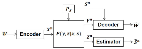
Figure 2: Two-receiver SDMC model.

We consider a two-receiver state-dependent memoryless channel (SDMC) and the corresponding information theoretic model is described as follows. A two-receiver SDMC model $\left(\mathcal{X},\mathcal{S},p\left(y,z|x,s\right),\mathcal{Y}\times\mathcal{Z}\right)$ consists of four finite sets $\mathcal{X},\mathcal{S},\mathcal{Y},\mathcal{Z}$ and a collection of conditional probability mass function (pmf) $p\left(y,z|x,s\right)$ on $\mathcal{Y}\times\mathcal{Z}$. As shown in Fig.2, the transmitter wants to send a message $W,W\in\left\{1,2,\cdots,2^{nR}\right\}$ to the ComRx over a state-dependent memoryless channel. At time $i$, we denote the channel input as $X_{i}\in\mathcal{X}$, the state as $S_{i}\in\mathcal{S}$, the SDMC transition probability as $P_{YZ|XS}(\cdot,\cdot|X_{i},S_{i})$, and the channel outputs as $Y_{i}\in\mathcal{Y}$ and $Z_{i}\in\mathcal{Z}$, respectively. The state sequence $S^{n}=(S_{1},\ldots,S_{n})$ is drawn i.i.d. according to a given state distribution $P_{S}(\cdot)$ and is perfectly known to the ComRx but unkown to the SenRx. Decoder at the ComRx finds the estimates $\hat{W}$ of the message to each received sequence $Y^{n}$ and Estimator at the SenRx estimates the state of the ComRx to received sequence $Z^{n}$.

A $\left(2^{n\mathrm{R}},n\right)$ code for the SDMC in the above model consists of

1) a message set $\left[1:2^{nR}\right]$;

2) an encoder that assigns a codeword $x^{n}(w)$ to each message $w\in\left[1:2^{nR}\right]$;

3) a decoder assigns an estimate $\hat{w}\in\left[1:2^{nR}\right]$ to each received sequence $y^{n}$;

4) a state estimator $h:\mathcal{Z}^{n}\rightarrow\mathcal{S}^{n}$, where Estimator estimates $\hat{s}^{n}=h(z^{n})$.

We assume that the random message $W$ is uniformly distributed over $\left[1:2^{nR}\right]$ and declare an error event as decoding error occurs in Decoder. Thus, the average probability of error is given by $P_{e}^{(n)}=\mathrm{Pr}\big{\{}\hat{W}\neq W\big{\}}$. The accuracy of the state estimation is measured by the expected average per-block distortion:

$$D^{(n)}:=\mathbb{E}\big{[}d(S^{n},\hat{S}^{n})\big{]}=\frac{1}{n}\sum_{i=1}^{n}\mathbb{E}\big{[}d(S_{i},\hat{S}_{i})\big{]},$$ (1)

where $d:\mathcal{S}\times\hat{\mathcal{S}}\mapsto\mathbb{R}^{+}$ is a given bounded distortion function with

$$d_{\max}=\max_{(s,\hat{s})\in\mathcal{S}\times\hat{\mathcal{S}}}d(s,\hat{s})<\infty.$$

A rate-distortion pair $(R,D)$ is said to be achievable if there exists a sequence of $\left(2^{nR},n\right)$ codes such that

$$\lim_{n\rightarrow\infty}P_{e}^{(n)}=0,$$ (2a)

$$\varlimsup_{n\rightarrow\infty}D^{(n)}\leq D,$$ (2b)

where $D$ is the desired maximum distortion. The capacity-distortion region of a two-receiver SDMC model is given by the closure of the union of all achievable rate-distortion pairs $(R,D)$.

II-B Two-receiver SDMBC-DMS model

In order to exploit communication to assist sensing, considering the broadcast channel model, i.e., the decoder at the SenRx can also decode the sent message to some degree, which can assist the state estimation of the SenRx. Without loss of generality, we can divide the message required by the ComRx into two non-overlapping parts; then the ComRx should recover both parts while the SenRx can recover the first part. We consider the case of unique decoding at the SenRx; i.e., the SenRx should decode the common part with vanishing error. Hence, this model could be seen as a two-receiver state-dependent memoryless broadcast channel with degraded message sets (SDMBC-DMS). Note that, different from the memoryless broadcast channel with degraded message sets [28], the SenRx should additionally estimate a state that is known by the ComRx.

Figure 3: Two-receiver SDMBC-DMS model.

The information theoretic model is described as follows. A two-receiver SDMBC-DMS model $\left(\mathcal{X},\mathcal{S},p\left(y,z|x,s\right),\mathcal{Y}\times\mathcal{Z}\right)$ consists of four finite sets $\mathcal{X},\mathcal{S},\mathcal{Y},\mathcal{Z}$ and a collection of conditional probability mass functions (pmf) $p\left(y,z|x,s\right)$ on $\mathcal{Y}\times\mathcal{Z}$. As shown in Fig. 3, the ISAC Tx sends a message $W=(W_{0},W_{1})$, where $W_{0}$ is the public message that can be decoded at both the ComRx and SenRx and $W_{1}$ is the private message that can be decoded at the ComRx only. Regarding the relationship between $W_{0}$ and $W$, there are three cases, i.e., $W_{0}=\emptyset$, $W_{0}\subset W$, and $W_{0}=W$, corresponding to three DnE strategies at the SenRx referred to as the blind estimation, the partial-decoding-based estimation and the full-decoding-based estimation, respectively. The message $W=(W_{0},W_{1})$ is encoded into a codeword $X^{n}$ and is transmitted over a two-receiver state-dependent discrete memoryless channel with i.i.d. state sequences. At time $i$, we denote the channel input as $X_{i}\in\mathcal{X}$, the state as $S_{i}\in\mathcal{S}$, the state-dependent memoryless channel transition probability as $P_{YZ|XS}(\cdot,\cdot|X_{i},S_{i})$, and the channel outputs as $Y_{i}\in\mathcal{Y}$ and $Z_{i}\in\mathcal{Z}$, respectively. The state sequence $S^{n}=(S_{1},\ldots,S_{n})$ is drawn i.i.d. according to a given state distribution $P_{S}(\cdot)$ and is perfectly known to the ComRx but unkown to the SenRx. Decoder 1 at the ComRx finds the estimates $\hat{W}_{01}$ and $\hat{W}_{1}$ of the common message and its private message to each received sequence $Y^{n}$, respectively. Decoder 2 at the SenRx finds the estimate $\hat{W}_{02}$ of the common message to each received sequence $Z^{n}$ and then estimates the state of the ComRx.

A $\left(2^{nR_{0}},2^{nR_{1}},n\right)$ code for SDMBC-DMS consists of

1) two message sets $\left[1:2^{nR_{0}}\right]$ and $\left[1:2^{nR_{1}}\right]$;

2) an encoder that assigns a codeword $x^{n}\left(w_{0},w_{1}\right)$ to each message pair $\left(w_{0},w_{1}\right)\in\left[1:2^{nR_{0}}\right]\times\left[1:2^{nR_{1}}\right]$;

3) two decoders, where Decoder 1 assigns an estimate $\left(\hat{w}_{01},\hat{w}_{1}\right)\in\left[1:2^{nR_{0}}\right]\times\left[1:2^{nR_{1}}\right]$ to each $(y^{n},s^{n})$ and Decoder 2 assigns an estimate $\hat{w}_{02}\in\left[1:2^{nR_{0}}\right]$ to each $z^{n}$;

4) a state estimator $h_{n}:\mathcal{Z}^{n}\rightarrow\mathcal{S}^{n}$, where Decoder 2 estimates $\hat{s}^{n}=h_{n}(z^{n})$.

We assume that the message pair $\left(W_{0},W_{1}\right)$ is uniformly distributed over $\left[1:2^{nR_{0}}\right]\times$ $\left[1:2^{nR_{1}}\right]$ and declare an error event as at least one decoding error occurs in Decoder 1 and Decoder 2. Thus, the average probability of error is given by

$$P_{1e}^{(n)}=\mathrm{Pr}\big{\{}(\hat{W}_{01},\hat{W}_{1})\neq\left(W_{0},W_{1}\right)\text{ or }\hat{W}_{02}\neq W_{0}\big{\}}.$$

A rate-distortion tuple $(R_{0},R_{1},D)$ is said to be achievable if there exists a sequence of $\left(2^{nR_{0}},2^{nR_{1}},n\right)$ codes such that

$$\lim_{n\rightarrow\infty}P_{1e}^{(n)}=0,$$ (3a)

$$\varlimsup_{n\rightarrow\infty}D^{(n)}\leq D,$$ (3b)

where $D$ is the desired maximum distortion. The capacity-distortion region of a SDMBC-DMS model is given by the closure of the union of all achievable rate-distortion tuples $(R_{0},R_{1},D)$. Note that, the total transmission rate for the ComRx is $R=R_{0}+R_{1}$.

Remark 1.

Note that for the model in Fig. 2, the option of rate splitting and partial decoding at the estimator is an achievable strategy, but not necessary for the problem definition. Instead, for the model in Fig. 3, we need to include the degraded message set condition as part of the problem definition. Thus, superposition encoding and partial decoding are common strategies for both problems, but error events are defined differently for the two problems. For the model in Fig. 2, the estimator does not care about the decoding of $W_{0}$. In contrast, for the model in Fig. 3, we require the estimator to be able to successfully decode $W_{0}$.

Remark 2.

From a practical application viewpoint, the degraded message set model is still quite relevant. For example, $W_{0}$ may be some common control information, and $W_{1}$ is the dedicated message for the communication receiver $(Y,S)$.

III Main results

In this section, we consider the rate-distortion region for the formulated SDMBC-DMS model with the proposed three DnE strategies. In particular, we further characterize the capacity region under the constraint of the degraded broadcast channel and the partial-decoding-based estimation.

III-A Rate-distortion region for the partial-decoding-based estimation

In this subsection, we consider the rate-distortion region for the formulated SDMBC-DMS model with the partial-decoding-based estimation strategy. We propose an achievable rate-distortion region given in the following theorem, whose proof could be found in Appendix B.

Theorem 1.

A rate-distortion tuple $(R_{0},R_{1},D)$ for the SDMBC-DMS system is achievable if

$$R_{0} \leq I\left(U;Z\right),$$ (4a)

$$R_{1} \leq I\left(X;Y|U,S\right),$$ (4b)

$$R_{0}+R_{1} \leq I\left(X;Y|S\right),$$ (4c)

for some $$P_{UX}(u,x)$$ satisfying

$$\sum_{u,x}P_{UX}(u,x)c^{*}(u)\leq D,$$ (4d)

where $c^{*}(u)=\mathrm{E}\left[d\big{(}S,\hat{s}^{*}(U,Z)\big{)}|U=u\right]$ and $\hat{s}^{*}(u,z)=\arg\min_{s^{\prime}\in\mathcal{S}}\sum_{s\in\mathcal{S}}P_{S|UZ}(s|u,z)d\left(s,s^{\prime}\right)$. The joint distribution of $SUXYZ$ is given by $P_{UX}P_{S}P_{YZ|XS}$ for some pmf $P_{UX}$, and the cardinality of the auxiliary random variable $U$ satisfies $\left|\mathcal{U}\right|\leq|\mathcal{X}|+1$.

Note that for the joint distribution of $SUXYZ$ is given by $P_{UX}P_{S}P_{YZ|XS}$, $\hat{s}^{*}(u,z)$ is the optimal one-shot state estimator, where the term ‘one-shot’ means that the estimator estimates the state $s_{i}$ in time slot $i$ only depending on $u_{i}$ and $z_{i}$. The proof on the optimality could be found in Appendix A.

Theorem 1 gives an achievable rate-distortion region of a two-receiver SDMBC-DMS model under the optimal one-shot state estimator, where $\hat{s}^{*}(u,z)$ can be interpreted as a minimizer of the penalty function on the distortion measure $d$ and $P_{S|UZ}(s|u,z)$ is the posterior probability of $S$ when $(U,Z)$ is known. In particular, when the distortion measure $d$ is the Hamming distance, $\hat{s}^{*}(u,z)$ is a maximum a posteriori probability estimate. In addition, (4a) can be understood as the rate at which the sensing receiver can reliably recover the common message, (4b) can be understood as the rate at which the communication receiver can reliably recover the private message, (4c) can be understood as the total rate at which the communication receiver can reliably recover all messages, and (4d) represents the desired distortion constraint. It is an open problem whether the optimal one-shot state estimator is generally optimal in our model or not.

Next, we propose a converse bound under the SDMBC-DMS system, whose proof could be found in Appendix D.

Theorem 2.

For the SDMBC-DMS system, if a rate-distortion tuple $(R_{0},R_{1},D)$ is achievable, then the following inequalities hold

$$R_{0} \leq I\left(U;Z\right),$$ (5a)

$$R_{1} \leq I\left(X;Y|U,S\right),$$ (5b)

$$R_{0}+R_{1} \leq I\left(X;Y|S\right),$$ (5c)

for some $$p(x)$$ satisfying

$$\sum_{x}P_{X}(x)\mathrm{E}\big{[}d\big{(}S,\hat{s}^{*}(X,Z)\big{)}|X=x\big{]}\leq D,$$ (5d)

where $\hat{s}^{*}(x,z)$ is the same as [25, Lemma 1] and the joint distribution of $SUXYZ$ is given by $P_{UX}P_{S}P_{YZ|XS}$ for some pmf $P_{UX}$.

Theorem 2 provides a genie-aided converse bound under the constraint of the partial-decoding-based estimation, where in the estimation step we construct a ‘stronger’ sensing user who perfectly knows $X$. Comparing the achievable bound in Theorem 1 and the converse bound in Theorem 2, we can find that the rate constraints (4a)-(4c) in Theorem 1 and (5a)-(5c) in Theorem 2 are the same, and the gap is mainly reflected in the distortion constraints. In addition, when the distortion constraint is not considered, i.e., $D\rightarrow\infty$, by combining the rate inequalities in Theorem 1 and Theorem 2, we can find that this is identical to the capacity region of the degraded message set where one output is $(Y,S)$ and the other is $Z$ which is known to be achieved by superposition coding.

III-B Capacity-distortion tradeoff for the degraded broadcast channel

In this subsection, we consider the degraded broadcast channel in which the ComRx is statistically stronger than the SenRx, specifically, $Z$ is a degraded form of $Y$; mathematically, $(X,S)-Y-Z$ forms a Markov chain. In this case, we have the following capacity result, whose proof could be found in Appendix E.

Theorem 3.

The capacity-distortion region $\left(C,D\right)$ for the SDMBC-DMS system where $(X,S)-Y-Z$ forms a Markov chain, is given by the closure of the set of all tuples $\left(R_{0},R_{1},D\right)$ that satisfy the rate constraints

$$\begin{split}R_{0}&\leq I\left(U;Z\right),\\ R_{1}&\leq I\left(X;Y|U,S\right),\\ \end{split}$$ (6)

for some $P_{UX}(u,x)$ satisfying

$$\sum_{u,x}P_{UX}(u,x)c^{*}(u)\leq D,$$

where the function $c^{*}(u)=\mathrm{E}\left[d\big{(}S,\hat{s}^{*}(U,Z)\big{)}\big{|}U=u\right]$. The joint distribution of $SUXYZ$ is given by $P_{UX}P_{S}P_{YZ|XS}$ for some pmf $P_{UX}$.

Theorem 3 gives the capacity-distortion region $\left(C,D\right)$ of the partial-decoding-based estimation in the case when $Z$ is a degraded form of $Y$. In this case, the optimal one-shot estimator outperforms estimators that depend on the output sequence. Intuitively speaking, in the case when $Z$ is a degraded form of $Y$, $Y$ contains more information about $X$ than $Z$. Compared to an estimator that only relies on the output sequence $Z^{n}$, the estimator in Theorem 3 uses not only $Z$ but also part of the information of $Y$ in the auxiliary variable $U$, leading to better estimates. In fact, using similar arguments, we can show that Theorem 3 also holds in the case where the Markov chain $X-(Y,S)-Z$ holds.

III-C Rate-distortion regions for the blind estimation and the full-decoding-based estimation

In this subsection, we discuss the cases of blind estimation, i.e., $R_{0}=0$ and full-decoding-based estimation, i.e., $R_{1}=0$. For both DnE strategies, we analyze the optimal estimators and corresponding rate-distortion regions, respectively.

In the case of blind estimation, we assume that the decoder at the SenRx does not decode any messages. In this case, the communication channel becomes a point-to-point state-dependent memoryless channel, which corresponds to the case where $R_{0}$ is equal to $0$ in Theorem 1 and the communication rate degenerates to $R_{1}$. For convenience, we use $R$ to represent the communication rate in the following. The optimal one-shot estimator with the assumption that the estimator knows the input distribution $P_{X}(x)$ is given by

$$\hat{s}^{*}(z)=\arg\min_{s^{\prime}\in\mathcal{S}}\sum_{s\in\mathcal{S}}P_{S|Z}(s|z)d\left(s,s^{\prime}\right),$$ (7)

where

$$P_{S|Z}(s|z)=\frac{P_{S}(s)\sum_{x\in\chi}P_{X}(x)P_{Z|XS}(z|x,s)}{\sum_{\tilde{s}\in\mathcal{S}}P_{S}(\tilde{s})\sum_{x\in\chi}P_{X}(x)P_{Z|XS}(z|x,\tilde{s})}.$$

Corollary 1.

A rate-distortion pair $(R,D)$ is achievable for the SDMBC-DMS system with the blind estimation if

$$R\leq I(X;Y|S)\ \text{and}\ \sum_{x\in\mathcal{X}}P_{X}(x)c_{1}(x)\leq D,$$ (8)

where $c_{1}(x)=\mathrm{E}\left[d\big{(}S,\hat{s}^{*}(Z)\big{)}|X=x\right]$ and the joint distribution of $SXYZ$ is given by $P_{X}P_{S}P_{YZ|XS}.$

Proof.

Similarly to the proof of Theorem 1, we use the estimator $\hat{S}^{n}=\big{(}\hat{s}^{*}(z_{1}),\hat{s}^{*}(z_{2}),\ldots,\hat{s}^{*}(z_{n})\big{)}$ and the details can be found in Appendix G. ∎

In the case of full-decoding-based estimation, we assume that the decoder at the SenRx can completely decode the sent message. In this case, the communication channel becomes a state-dependent memoryless broadcast channel with only public messages, which corresponds to the case where $R_{1}$ is equal to $0$ in Theorem 1 and the communication rate degenerates to $R_{0}$. The optimal estimator in this case has been studied in [25, Lemma 1] and it is given by

$$\hat{s}^{*}(x,z)=\arg\min_{s^{\prime}\in\hat{\mathcal{S}}}\sum_{s\in\mathcal{S}}P_{S|XZ}(s|x,z)d\left(s,s^{\prime}\right).$$ (9)

We use $C=R_{0}$ to represent the channel capacity and have the following result.

Corollary 2.

The capacity-distortion tradeoff for the SDMBC-DMS system with the full-decoding-based estimation is given by

$$C(D)=\max_{P_{X}\in\mathcal{P}_{D}}\min\{I(X;Y|S),I(X;Z)\},$$ (10)

where $\mathcal{P}_{D}=\{P_{X}|\sum_{x\in\mathcal{X}}P_{X}(x)c(x)\leq D\},c(x)=\mathrm{E}\big{[}d\big{(}S,\hat{s}^{*}(X,Z)\big{)}|X=x\big{]}$, and the joint distribution of $SXYZ$ is given by $P_{X}P_{S}P_{YZ|XS}.$

Proof.

We use the estimator $\hat{S}^{n}=\big{(}\hat{s}^{*}(\hat{x}_{1},z_{1}),\hat{s}^{*}(\hat{x}_{2},z_{2}),\ldots,\hat{s}^{*}(\hat{x}_{n},z_{n})\big{)}$ to get the achievability proof as in the proof of Theorem 1. The converse proof is similar to that of [34, Theorem 1] by noting that the one-shot estimator in this case is the global optimal estimator. The details can be found in Appendix H. ∎

IV Examples

In this section, we provide a specific non-degraded example and a degraded example to illustrate explicitly the results in the previous section.

1) Example 1: The non-degraded broadcast channel

In this example, we consider a binary communication channel with a multiplicative Bernoulli state, where the signal received by the ComRx is given by $Y=SX$ with binary alphabets $\mathcal{X}=\mathcal{S}=\mathcal{Y}=\{0,1\}$ and the state $S$ is Bernoulli$(q)$, for $q\in(0,1)$. The signal received by the SenRx is expressed as the sum of two parts, where one part is the signal reflected by the ComRx and the other part is the directly radiated signal by of the ISAC Tx. The first part can be expressed as the product of a binary channel with a multiplicative Bernoulli state and an attenuation factor $a\in(0,1)$ and the second part can be expressed as a binary symmetric channel $\big{(}\mathrm{BSC}(e)\big{)}$ with error probability $e\in[0,1]$. Hence, the sensing channel can be expressed as $Z=aSX+(X+N)\mod 2$ with alphabets $\mathcal{Z}=\{0,1,a,a+1\}$, where $a\in(0,1)$, $N$ is Bernoulli$(e)$, and $e\in[0,1]$. We consider the Hamming distortion measure $d(s,\hat{s})=s\oplus\hat{s}$ to characterize the sensing accuracy.

We apply the outer bound and the three DnE strategies to Example 1, and the results are shown in Corollaries 3 - 6 below where, unless otherwise stated, $\bar{e}$ represents $1-e$ and $H_{2}(p)=-p\log_{2}p-(1-p)\log_{2}(1-p)$ represents a binary entropy function with $p\in[0,1]$.

Corollary 3.

In Example 1, a converse bound on $C(D)$ is given by

$$R_{0}+R_{1}=\min\{qH_{2}(p),I\left(U;Z\right)+I\left(X;Y|U,S\right)\}\ \text{and}\ D=p\min\{q,1-q\}.$$

Proof.

See Appendix I. ∎

Based on Theorem 2, Corollary 3 gives an outer bound with the partial-decoding-based estimation strategy in Example 1.

Corollary 4.

In Example 1, an achievable rate-distortion region with the partial-decoding-based estimation is given by

$$R_{0}+R_{1} =\min\{qH_{2}(p),I\left(U;Z\right)+I\left(X;Y|U,S\right)\}$$

$$D =\sum_{i=0}^{1}\sum_{j=0}^{2}p(z=i,u=j)d_{ij},$$

where $d_{0j}$ and $d_{1j}$ are given in (33) and (34), respectively.

Proof.

See Appendix J. ∎

Based on Theorem 1, Corollary 4 gives an achievable rate-distortion region with the partial decoding estimation strategy in Example 1.

Corollary 5.

In Example 1, an achievable rate-distortion region with the blind estimation is given by

$$R=qH_{2}(p)\ \text{and}\ D=d_{11}+d_{12},$$

where $d_{11}$ and $d_{12}$ are given in (39) and (40), respectively.

Proof.

See Appendix K. ∎

Based on Corollary 1, Corollary 5 gives an achievable rate-distortion region with the blind estimation strategy in Example 1. For the case of blind estimation, only the ComRx needs to decode the information and thus there is only one rate component.

Corollary 6.

In Example 1, the capacity-distortion region with the full-decoding-based estimation is given by

$$C(D) =\min\{qH_{2}(p),I(X;Z)\},\ D=p\min\{q,1-q\},\ \text{and}$$

$$I(X;Z) =-\sum_{i=1}p_{i}\log_{2}p_{i}-pH_{2}(e)+\bar{p}\sum_{i=1}p_{i1}\log_{2}p_{i1},$$

where $p_{1}=pe+\bar{q}\bar{p}\bar{e},p_{2}=p\bar{e}+\bar{q}\bar{p}e,p_{3}=\bar{p}qe,p_{4}=\bar{p}q\bar{e},p_{11}=\bar{q}\bar{e},p_{21}=\bar{q}e,p_{31}=qe,p_{41}=q\bar{e}.$ In other words, the curve $C(D)$ is parameterized as

$$\left\{\left(C=\min\{qH_{2}(p),I(X;Z)\},D\right):p\in[0,p_{\max}]\right\}$$

where $p_{\max}$ is the input probability that maximizes $C(D)$.

Proof.

See Appendix L. ∎

Based on Corollary 2, Corollary 6 gives an achievable rate-distortion region with the full-decoding-based estimation strategy in Example 1. We observe that the expressions of the distortion $D$ in Corollary 6 and Corollary 3 are the same since the estimators rely on the same information $(X,Z)$, where the estimator in Corollary 6 obtains the information of $X$ by decoding, and the estimator in Corollary 3 obtains the information of $X$ by the construction of genie.

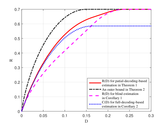
Figure 4: Rate-distortion regions for three DnE strategies and an outer bound of the rate-distortion region with parameters $e=0.25$ and $q=0.7$ in Example 1.

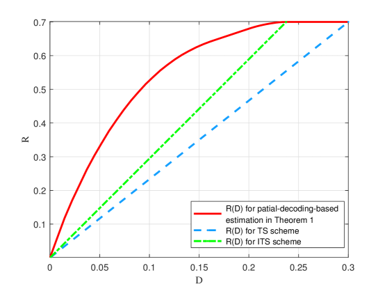
Figure 5: Rate-distortion regions of the partial-decoding-based estimation and two time-sharing schemes with parameters $e=0.25$ and $q=0.7$ in Example 1.

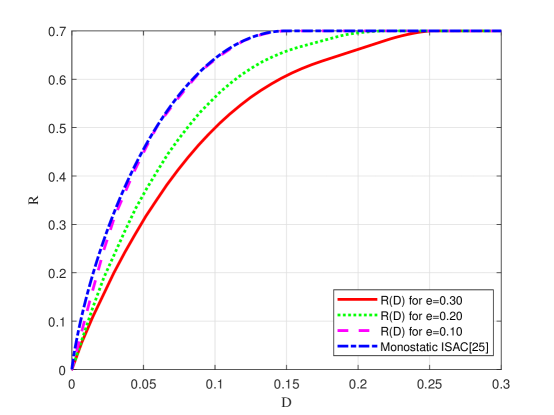
Figure 6: Rate-distortion regions of the partial-decoding-based estimation for different values of $e$ with parameters $q=0.7$ in Example 1.

We consider $e=0.25$ and $q=0.7$ and plot the rate-distortion regions in Corollaries 3 - 6 in Fig. 4. It is shown that, the regions of the blind estimation and the full-decoding-based estimation are strictly within the rate-distortion region of the partial-decoding-based estimation, as expected. Also, Corollary 3 provides an outer bound on $C(D)$, where the estimator has a prior of $X$, which is on the upper left of the curves of the three DnE strategies.

In Fig. 5, we compare the performance of the proposed partial-decoding-based estimation strategy, the basic time-sharing scheme (TS), and the improved time-sharing scheme (ITS). The TS scheme refers to independent communication and sensing in a time-sharing manner. In the basic TS scheme, the minimum distortion $D_{\min}=0$ is achieved always by sending $X=1$, i.e., $P(x=1)=1$ and $P(x=0)=0$. Furthermore, we can obtain $R_{\min}=0$, $R_{\max}=0.7$, and $D_{\max}=\min\{q,1-q\}$ by using the best constant estimator, $\hat{s}=\operatorname{argmax}_{s\in\{0,1\}}P_{S}(s)$. The basic TS scheme thus achieves the straight line between $(0,0)$ and $(0.3,0.7)$. The ITS scheme simultaneously performs communication and sensing tasks, while the input distribution is optimized for either sensing or communication. It enables all rate-distortion pairs between two points, one for sensing with an input distribution that maximizes the communication rate and the other for communicating with an input distribution that minimizes distortion. Specifically, in the ITS scheme, the minimum distortion is $D_{\min}=0$, in which case $R_{\min}=0$. Furthermore, we can obtain $R_{\max}=0.7$ and find the distribution that realizes $R_{\max}$ and thus obtain the corresponding distortion $D_{\max}=0.2375$ from Corollary 4. The ITS scheme thus achieves the straight line between $(0,0)$ and $(0.2375,0.7)$. We can observe a significant gain of the proposed strategy over the two baseline TS schemes. The performance gap between the TS scheme and the ITS scheme indicates the integration gain of ISAC [10]. The performance gap between the ITS scheme and the proposed strategy indicates the gain of joint design of the input distribution and the DnE strategy.

In Fig. 6, we plot the rate-distortion region of the partial-decoding-based estimation for different values of $e\in(0,1/2)$, which measures the channel quality from the ISAC Tx to the SenRx. Besides, we also plot the rate-distortion of the monostatic ISAC system studied in [25] that corresponds to the case of the state $S$ is estimated from $Z=Y=SX$ at the ISAC Tx. It is seen that the smaller the value of $e$, the higher the curve, i.e., the greater the corresponding rate under the same distortion. When the value of $e$ is slightly larger, such as $0.30$ or $0.20$, the rate-distortion performance of the bistatic ISAC system is worse than that of the monostatic ISAC system. This is because a slightly larger value of $e$ means that the direct link channel quality deteriorates. Therefore, the performance gain of communication-assisted sensing degrades and thus the distortion in the bistatic ISAC system becomes larger when the same rate is reached. Interestingly, as $e<0.1$, the rate-distortion of the bistatic ISAC system matches that of the monostatic ISAC system closely [25], which implies that the performance of the bistatic ISAC system approaches that of the monostatic ISAC system when the direct link channel is modestly accurate. In fact, it is worth noting that the capacity-distortion performance of the monostatic ISAC system derived in [25] is usually over optimistic since the self-interference, which must exist in the monostatic system, has not been taken into account in [25].

2) Example 2: The degraded broadcast channel

We further simplify Example 1 to obtain Example 2. In particular, we change the sensing channel to $Z=aY+(Y+N)\mod 2=aSX+(SX+N)\mod 2$ with alphabets $\mathcal{Z}=\{0,1,a,a+1\}$, where $a\in(0,1)$, $N$ is Bernoulli$(e)$, and $e\in[0,1]$ in order to ensure that $Z$ is a degraded form of $Y$. Also, we can get the rate-distortion expressions corresponding to the three DnE strategies in Appendix M and the corresponding three curves in Fig. 7.

In Fig. 7, it is observed that in the degraded broadcast channel, the curve corresponding to the partial-decoding-based estimation is the capacity-distortion curve, which is located at the upper left of the rate-distortion curves of the blind estimation and the capacity-distortion curve of the full-decoding-based estimation.

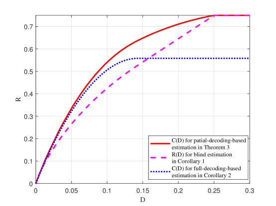
Figure 7: Rate-distortion regions for three DnE strategies with parameters $e=0.25$ and $q=0.75$ in Example 2.

V Conclusion

In this paper, we considered a bistatic ISAC system without self-interference and characterized its rate-distortion or capacity-distortion regions with three DnE strategies. Besides, for the partial-decoding-based estimation strategy at the SenRx, we also characterized the capacity-distortion region under the degraded broadcast channel in which the ComRx is statistically stronger than the SenRx. A non-degraded example and a degraded illustrative example were given to show the relationship among the three DnE strategies and the benefits of bistatic ISAC compared to the two baseline time-sharing schemes. We found that 1) dynamically selecting the amount of information to be decoded for assisting sensing outperforms the blind estimation and the full-decoding-based estimation; 2) the bistatic ISAC system requires the joint design of the input distribution and the DnE strategy to improve the tradeoff between communication and sensing.

Appendix A Proof of the optimal one-shot state estimator

According to (1) and the law of total expectation, we have

$$\quad\ \mathbb{E}\big{[}d\big{(}S_{i},\hat{S}_{i}(U_{i},Z_{i})\big{)}\big{|}U_{i}=u_{i}\big{]}$$

$$=\sum_{z_{i},\hat{s},s}P_{Z_{i}|U_{i}}P_{\hat{S}_{i}|U_{i}Z_{i}}P_{S_{i}|U_{i}Z_{i}}d(s,\hat{s})$$

$$\geq\sum_{z_{i}}P_{Z_{i}|U_{i}}\min_{\hat{s}\in\mathcal{S}}\sum_{s}P_{S_{i}|U_{i}Z_{i}}d(s,\hat{s})$$

$$\stackrel{{\scriptstyle(\mathrm{a})}}{{=}}\sum_{z_{i}}P_{Z_{i}|U_{i}}P_{S_{i}|U_{i}Z_{i}}d\big{(}s,\hat{s}^{*}(u_{i},z_{i})\big{)}$$

$$=\mathbb{E}\big{[}d\big{(}S_{i},\hat{s}^{*}(U_{i},Z_{i})\big{)}\big{|}U_{i}=u_{i}\big{]},$$

which yields the desired conclusion, where $(a)$ holds by choosing $\hat{s}^{*}(u,z)$ in Theorem 1.

Appendix B Proof of Theorem 1

The proof is mainly divided into two parts: the rate expressions and the state distortion constraint.

a) Codebook generation. Fix a pmf $p(u)p(x|u)$ such that the expected distortion is less than $\left(D/(1+\epsilon)\right)$ for a small positive number $\epsilon>0$, where $D$ is the desired distortion. Randomly and independently generate $2^{nR_{0}}$ sequences $u^{n}\left(w_{0}\right),w_{0}\in\left[1:2^{nR_{0}}\right]$, each according to $\prod_{i=1}^{n}p_{U}(u_{i})$. For each $w_{0}\in$ $\left[1:2^{nR_{0}}\right]$, randomly and conditionally independently generate $2^{nR_{1}}$ sequences $x^{n}\left(w_{0},w_{1}\right)$, $w_{1}\in\left[1:2^{nR_{1}}\right]$, each according to $\prod_{i=1}^{n}p_{X|U}\big{(}x_{i}|u_{i}(w_{0})\big{)}$.

b) Encoding. To send $\left(w_{0},w_{1}\right)$, transmit $x^{n}\left(w_{0},w_{1}\right)$.

c) Decoding. Decoder 2 declares that $\hat{w}_{02}$ is sent if it is the unique message such that $\left(u^{n}\left(\hat{w}_{02}\right)\right.$, $\left.z^{n}\right)\in\mathcal{T}_{\epsilon}^{(n)}(P_{UZ})$, where $\mathcal{T}_{\epsilon}^{(n)}$ refers to jointly $\epsilon$-typical sequences; otherwise it declares an error. Decoder 1 declares that $(\hat{w}_{01},\hat{w}_{1})$ is sent if it is the unique message pair such that $\big{(}{u^{n}(\hat{w}_{01})},x^{n}(\hat{w}_{01},\hat{w}_{1}),y^{n},s^{n}\big{)}\in\mathcal{T}_{\epsilon}^{(n)}(P_{UXYS})$; otherwise it declares an error.

d) Estimation. Assuming that the sensing channel output is $Z^{n}=z^{n}$ and the decoded information is $\hat{U}^{n}=\hat{u}^{n}$, then the one-shot estimator gives the estimation of the state sequences

$$\hat{S}^{n}=\big{(}\hat{s}^{*}(\hat{u}_{1},z_{1}),\hat{s}^{*}(\hat{u}_{2},z_{2}),\ldots,\hat{s}^{*}(\hat{u}_{n},z_{n})\big{)}.$$

e) Analysis of the probability of error. Assume without loss of generality that $\left(W_{0},W_{1}\right)=(1,1)$ is sent. The average probability of error is

$$P_{1e}^{(n)}=\mathrm{P}\big{\{}(\hat{W}_{01},\hat{W}_{1})\neq\left(1,1\right)\text{ or }\hat{W}_{02}\neq 1\big{\}}.$$

First consider the average probability of error for decoder 2 at the SenRx. Define $\mathcal{E}_{0}$ as an error in Decoder 2 that occurs if and only if one or both of the following events occur:

$$\mathcal{E}_{01}=\left\{\left(U^{n}(1),Z^{n}\right)\notin\mathcal{T}_{\epsilon}^{(n)}(P_{UZ})\right\}\ \text{and}$$

$$\mathcal{E}_{02}=\left\{\left(U^{n}\left(w_{02}\right),Z^{n}\right)\in\mathcal{T}_{\epsilon}^{(n)}(P_{UZ})\text{ for some }w_{02}\neq 1\right\}.$$

Thus, the probability of error for decoder 2 is upper bounded as

$$\mathrm{P}\left(\mathcal{E}_{0}\right)\leq\mathrm{P}\left(\mathcal{E}_{01}\right)+\mathrm{P}\left(\mathcal{E}_{02}\right).$$

By the law of large numbers (LLN), the first term $\mathrm{P}\left(\mathcal{E}_{01}\right)$ tends to zero as $n\rightarrow\infty$. For the second term, since $U^{n}\left(w_{02}\right)$ is independent of $\big{(}U^{n}(1),Z^{n}\big{)}$ for $w_{02}\neq 1$, by the packing lemma[29, Lemma 3.1], $\mathrm{P}\left(\mathcal{E}_{02}\right)$ tends to zero as $n\rightarrow\infty$ if $R_{0}<I\left(U;Z\right)-\delta(\epsilon),$ where $\delta(\epsilon)\rightarrow 0$ when $n\rightarrow\infty$.

Next, we consider the average probability of error for decoder 1 at the ComRx. Define $\mathcal{E}_{1}$ as an error in Decoder 1 that occurs if and only if one or more of the following four events occur:

$$\mathcal{E}_{11}=\big{\{}\big{(}U^{n}(1),X^{n}(1,1),Y^{n},S^{n}\big{)}\notin\mathcal{T}_{\epsilon}^{(n)}(P_{UXYS})\big{\}},$$

$$\mathcal{E}_{12}=\big{\{}\big{(}U^{n}(1),X^{n}(1,w_{1}),Y^{n},S^{n}\big{)}\in\mathcal{T}_{\epsilon}^{(n)}(P_{UXYS})\text{ for some }w_{1}\neq 1\big{\}},$$

$$\mathcal{E}_{13}=\big{\{}\big{(}U^{n}(w_{0}),X^{n}(w_{0},1),Y^{n},S^{n}\big{)}\in\mathcal{T}_{\epsilon}^{(n)}(P_{UXYS})\text{ for some }w_{0}\neq 1\big{\}},\ \text{and}$$

$$\mathcal{E}_{14}=\big{\{}\big{(}U^{n}(w_{0}),X^{n}(w_{0},w_{1}),Y^{n},S^{n}\big{)}\in\mathcal{T}_{\epsilon}^{(n)}(P_{UXYS})\text{ for some }w_{0}\neq 1,w_{1}\neq 1\big{\}}.$$

Thus, the probability of error for decoder 1 is upper bounded as

$$\mathrm{P}\left(\mathcal{E}_{1}\right)\leq\mathrm{P}\left(\mathcal{E}_{11}\right)+\mathrm{P}\left(\mathcal{E}_{12}\right)+\mathrm{P}\left(\mathcal{E}_{13}\right)+\mathrm{P}\left(\mathcal{E}_{14}\right).$$

By the LLN, $\mathrm{P}\left(\mathcal{E}_{11}\right)$ tends to zero as $n\rightarrow\infty$. For the second term, note that if $w_{1}\neq 1$, then $X^{n}\left(1,w_{1}\right)$ is conditionally independent of $\left(X^{n}(1,1),Y^{n},S^{n}\right)$ given $U^{n}(1)$ and is distributed according to $\prod_{i=1}^{n}p_{X|U}\left(x_{i}|u_{i}(1)\right)$. So, by the packing lemma and independence of $(U,X)$ and $S$, $\mathrm{P}\left(\mathcal{E}_{12}\right)$ tends to zero as $n\rightarrow\infty$ if $R_{1}<I\left(X;Y,S|U\right)-\delta(\epsilon)=I\left(X;Y|S,U\right)-\delta(\epsilon)$. For the third term, note that for $w_{0}\neq 1$, $\left(U^{n}\left(w_{0}\right),X^{n}\left(w_{0},1\right)\right)$ is independent of $\left(U^{n}(1),X^{n}(1,1),Y^{n},S^{n}\right)$. Hence, by the packing lemma and Markov chain: $U\rightarrow X\rightarrow Y$, $\mathrm{P}\left(\mathcal{E}_{13}\right)$ tends to zero as $n\rightarrow\infty$ if $R_{0}<I\left(U,X;Y,S\right)-\delta(\epsilon)=I\left(X;Y,S\right)-\delta(\epsilon)=I\left(X;Y|S\right)-\delta(\epsilon)$. For the last term, note that for $w_{0}\neq 1$ and any $w_{1},\left(U^{n}\left(w_{0}\right),X^{n}\left(w_{0},w_{1}\right)\right)$ is independent of $\left(U^{n}(1),X^{n}(1,1),Y^{n},S^{n}\right)$. Hence, by the packing lemma, $\mathrm{P}\left(\mathcal{E}_{14}\right)$ tends to zero as $n\rightarrow\infty$ if $R_{0}+R_{1}<I\left(U,X;Y,S\right)-\delta(\epsilon)=I\left(X;Y|S\right)-\delta(\epsilon)$. Therefore, we get that $\mathrm{P}\left(\mathcal{E}_{1}\right)$ tends to zero as $n\rightarrow\infty$ if $R_{1}<I\left(X;Y,S|U\right)-\delta(\epsilon)=I\left(X;Y|U,S\right)-\delta(\epsilon)$ and $R_{0}+R_{1}<I\left(X;Y|S\right)-\delta(\epsilon)$ hold, where $\delta(\epsilon)\rightarrow 0$ when $n\rightarrow\infty$. Thus, we get the rate expressions in (4).

f) Analysis of the expected distortion

Inspired by the proof of [25, Theorem 1], we define the correct decoding event as $\mathcal{A}=\big{\{}(\hat{W}_{01},\hat{W}_{1})=(1,1)\text{ and }\hat{W}_{02}=1\big{\}}$ and the complement of $\mathcal{A}$ as $\mathcal{A}^{c}$. The expected distortion (averaged over the random codebook, state and channel noise) can be upper bounded by

$$D^{(n)} =\frac{1}{n}\sum_{i=1}^{n}\mathrm{E}\big{[}d(S_{i},\hat{S}_{i})\big{]}$$

$$=\frac{1}{n}\operatorname{P}(\mathcal{A}^{c})\sum_{i=1}^{n}\mathrm{E}\big{[}d(S_{i},\hat{S}_{i})\big{|}\mathcal{A}^{c}\big{]}+\frac{1}{n}\operatorname{P}(\mathcal{A})\sum_{i=1}^{n}\mathrm{E}\big{[}d(S_{i},\hat{S}_{i})\big{|}\mathcal{A}\big{]}$$

$$\leq d_{\max}P_{1e}^{(n)}+\frac{1}{n}\sum_{i=1}^{n}\mathrm{E}\big{[}d(S_{i},\hat{S}_{i})\big{|}\mathcal{A}\big{]}(1-P_{1e}^{(n)}).$$ (11)

According to the decoding principle of both decoders, in the event of correct decoding, we have

$$\big{(}U^{n}(1),X^{n}(1,1),Y^{n},S^{n}\big{)}\in\mathcal{T}_{\epsilon}^{(n)}\left(P_{UX}P_{S}P_{Y|SX}\right)$$

and

$$\big{(}U^{n}(1),Z^{n}\big{)}\in\mathcal{T}_{\epsilon}^{(n)}\left(P_{U}P_{Z|U}\right).$$

Furthermore, according to the fact that $\hat{S}_{i}=\hat{s}^{*}\left(U_{i},Z_{i}\right)$ in the event of correct decoding and the conditional typicality lemma [29, Lemma 2.5], we get for every $\epsilon^{\prime}>\epsilon$,

$$P\Big{(}\big{(}S^{n},U^{n}(1),\hat{S}^{n}\big{)}\in\mathcal{T}_{\epsilon^{\prime}}^{(n)}(P_{SU\hat{S}})\Big{)}=1-\eta,$$

where $P_{SU\hat{S}}$ denotes the joint marginal distribution of $P_{SUXZ\hat{S}}(s,u,x,z,\hat{s})=P_{UX}(u,x)\cdot P_{S}(s)\cdot$ $P_{Z|SX}(z|s,x)\cdot{\bf{{1}}}\left\{\hat{s}=\hat{s}^{*}(u,z)\right\}$, ${\bf{1}}(\cdot)$ is the indicative function, $\eta\in(0,1)$ and $\lim_{n\to\infty}\eta=0$. Then, we define $(S^{n},U^{n}(1),\hat{S}^{n})\in\mathcal{T}_{\epsilon^{\prime}}^{(n)}(P_{SU\hat{S}})$ as event $\mathcal{B}$ and the complement of $B$ as $\mathcal{B}^{c}$. According to the typical average lemma [29], we get

$$\quad\ \varlimsup_{n\rightarrow\infty}\frac{1}{n}\sum_{i=1}^{n}\mathrm{E}\big{[}d(S_{i},\hat{S}_{i})\big{|}\mathcal{A}\big{]}$$

$$=\varlimsup_{n\rightarrow\infty}\frac{1}{n}(1-\eta)\sum_{i=1}^{n}\mathrm{E}\big{[}d(S_{i},\hat{S}_{i})\big{|}\mathcal{A},\mathcal{B}\big{]}+\varlimsup_{n\rightarrow\infty}\frac{1}{n}\eta\sum_{i=1}^{n}\mathrm{E}\big{[}d(S_{i},\hat{S}_{i})\big{|}\mathcal{A},\mathcal{B}^{c}\big{]}$$

$$\leq\varlimsup_{n\rightarrow\infty}(1-\eta)(1+{\epsilon^{\prime}})\mathrm{E}[d(S,\hat{S})]+\eta d_{\max}$$

$$=(1+{\epsilon^{\prime}})\mathrm{E}[d(S,\hat{S})]$$ (12)

for $(S,\hat{S})$ following the joint marginal distribution of $P_{SUZ\hat{S}}$ defined above. Assuming that (4) holds and thus $P_{1e}\rightarrow 0$ as $n\rightarrow\infty$, we obtain from (B) and (B) that

$$\varlimsup_{n\rightarrow\infty}D^{(n)}\leq(1+{\epsilon^{\prime}})\mathrm{E}[d(S,\hat{S})].$$

Taking ${\epsilon^{\prime}}\rightarrow\epsilon$, we can conclude that the error probability vanishes and the distortion constraint holds when (4) holds and $\mathrm{E}[d(S,\hat{S})]<D/(1+\epsilon).$ Besides, according to the cardinality bounding technique in [29, Appendix C] and considering the state variable $S$, we can get the cardinality of the auxiliary random variable $U$ and the details can be found in Appendix C.

Appendix C Proof of the cardinality of the auxiliary random variable U

Let $U\sim F(u)$ and $X|\{U=u\}\sim p(x|u)$, where $U$ takes values in an arbitrary set $\mathscr{U}$. Let $\mathscr{R}(U,X)$ be the set of rate pairs $\left(R_{0},R_{1}\right)$ such that

$$R_{0} \leq I\left(U;Z\right),$$

$$R_{1} \leq I\left(X;Y|U,S\right),\ \text{and}$$

$$R_{0}+R_{1} \leq I\left(X;Y|S\right),$$

We prove that given any $(U,X)$, there exists $\left(U^{\prime},X\right)$ with $\left|\mathcal{U}^{\prime}\right|\leq|\mathcal{X}|+1$ such that $\mathscr{R}(U,X)=\mathscr{R}\left(U^{\prime},X\right)$, which implies that it suffices to consider auxiliary random variables with $\left|\mathcal{U}\right|\leq|\mathcal{X}|+1$.

Assume without loss of generality that $\mathcal{X}=\{1,2,\ldots,|\mathcal{X}|\}$. Since $X$ and $S$ are independent, and $S\sim p_{S}(\cdot)$ is given, consider the set $\mathscr{P}$ of all pmfs on $\mathcal{X}$ (which is connected and compact) for a given $(U,X)$, and the following $|\mathcal{X}|+1$ continuous functions on $\mathscr{P}$:

$$g_{j}(\pi)=\begin{cases}\pi(j)&j=1,\ldots,|\mathcal{X}|-1,\\ H\left(Y|S\right)&j=|\mathcal{X}|,\\ H\left(Z\right)&j=|\mathcal{X}|+1.\end{cases}$$

Clearly, the first $|\mathcal{X}|-1$ functions are continuous. The last two functions are also continuous in $\pi$ by continuity of the entropy function and linearity of $p\left(y|s\right)=\sum_{x}p\left(y|x,s\right)\pi(x)$ and $p\left(z\right)=\sum_{x}p\left(z|x,s\right)p(s)\pi(x)$ in $\pi$. Now by the support lemma [29, Appendix C], we can find a random variable $U^{\prime}$ taking at most $|\mathcal{X}|+1$ values such that

$$H\left(Y|S,U\right) =\int_{\mathscr{U}}H\left(Y|S,U=u\right)dF(u)$$

$$=\sum_{u^{\prime}}H\left(Y|S,U^{\prime}=u^{\prime}\right)p\left(u^{\prime}\right)$$

$$=H\left(Y|S,U^{\prime}\right),$$

$$H\left(Z|U\right) =\int_{\mathscr{U}}H\left(Z|U=u\right)dF(u)$$

$$=\sum_{u^{\prime}}H\left(Z|U^{\prime}=u^{\prime}\right)p\left(u^{\prime}\right)$$

$$=H\left(Z|U^{\prime}\right),\ \text{and}$$

$$\int_{\mathscr{U}}p(s)p(x|u)dF(u) =p(s)p(x)=\sum_{u^{\prime}}p(s)p_{X|U}\left(x|u^{\prime}\right)p\left(u^{\prime}\right),$$

for $x=1,\ldots,|\mathcal{X}|-1$ and hence for $x=|\mathcal{X}|$. Since $p(x)p(s)$ is preserved and $p(x)p(s)$ determines $p\left(x,s,y\right)=p(x)p(s)p\left(y|s,x\right)$, $p\left(s,y\right)=\sum_{x}p(x)p(s)p\left(y|s,x\right)$ and $p\left(z\right)=\sum_{x,s}p(x)p(s)$ $p\left(z|x,s\right)$, $H\left(Y|X,S\right)$, $H\left(Y|S\right)$ and $H\left(Z\right)$ are also preserved, and

$$I\left(U;Z\right) =H\left(Z\right)-H\left(Z|U\right)=H\left(Z\right)-H\left(Z|U^{\prime}\right)=I\left(U^{\prime};Z\right),$$

$$I\left(X;Y|S\right) =H\left(Y|S\right)-H\left(Y|X,S\right)=I\left(X;Y|S\right),$$

$$I\left(X;Y|U,S\right) =H\left(Y|U,S\right)-H\left(Y|X,S\right)=H\left(Y|U^{\prime},S\right)-H\left(Y|X,S\right)=I\left(X;Y|U^{\prime},S\right).$$

Thus, we have shown that $\mathscr{R}(U,X)=\mathscr{R}\left(U^{\prime},X\right)$ for some $U^{\prime}$ with $\left|\mathcal{U}^{\prime}\right|\leq|\mathcal{X}|+1$.

Appendix D Proof of Theorem 2

It is difficult to find an identification of the auxiliary random variable that satisfies the desired properties for the capacity region characterization in (5). Instead, we prove the converse for the equivalent region consisting of all rate pairs $\left(R_{0},R_{1}\right)$ such that

$$R_{0} \leq I\left(U;Z\right),$$

$$R_{0}+R_{1} \leq I\left(X;Y|U,S\right)+I\left(U;Z\right),\ \text{and}$$

$$R_{0}+R_{1} \leq I\left(X;Y|S\right),$$

for some $\operatorname{pmf}p(u,x)$. The proof of equivalence of regions is shown in Appendix F.

According to Fano’s inequality [29] and the fact that decoder 1 in the SDMBC-DMS model can fully decode the message $\left(W_{0},W_{1}\right)$, we have $H\left(W_{1}|Y^{n},S^{n}\right)\leq n\epsilon_{n},H\left(W_{0}|Z^{n}\right)\leq n\epsilon_{n}$ and $H\left(W_{0},W_{1}|Y^{n},S^{n}\right)\leq n\epsilon_{n}$ for some $\epsilon_{n}$ that tends to zero as $n\rightarrow\infty$. Hence, we have

$$\begin{split}nR_{0}\leq&\ I\left(W_{0};Z^{n}\right)+n\epsilon_{n},\\ n\left(R_{0}+R_{1}\right)\leq&\ I\left(W_{1};Y^{n},S^{n}|W_{0}\right)+I\left(W_{0};Z^{n}\right)+n\epsilon_{n},\ \text{and}\\ n\left(R_{0}+R_{1}\right)\leq&\ I\left(W_{0},W_{1};Y^{n},S^{n}\right)+n\epsilon_{n}.\end{split}$$ (13)

In the following, we omit the $n\epsilon_{n}$ terms. From the second inequality in (13), we have

$$\quad\ n\left(R_{0}+R_{1}\right)-n\epsilon_{n}$$

$$\leq I\left(W_{1};Y^{n},S^{n}|W_{0}\right)+I\left(W_{0};Z^{n}\right)$$

$$\stackrel{{\scriptstyle(a)}}{{=}}\sum_{i=1}^{n}I\left(W_{1};Y_{i},S_{i}|W_{0},Y^{i-1},S^{i-1}\right)+I\left(W_{0};Z_{i}|Z_{i+1}^{n}\right)$$

$$\leq\sum_{i=1}^{n}I\left(W_{1},Z_{i+1}^{n};Y_{i},S_{i}|W_{0},Y^{i-1},S^{i-1}\right)+I\left(W_{0},Z_{i+1}^{n};Z_{i}\right)$$

$$=\sum_{i=1}^{n}I\left(W_{1},Z_{i+1}^{n};Y_{i},S_{i}|W_{0},Y^{i-1},S^{i-1}\right)+I\left(W_{0},Z_{i+1}^{n},Y^{i-1},S^{i-1};Z_{i}\right)-I\left(Y^{i-1},S^{i-1};Z_{i}|W_{0},Z_{i+1}^{n}\right)$$

$$=\sum_{i=1}^{n}I\left(W_{1};Y_{i},S_{i}|W_{0},Y^{i-1},S^{i-1},Z_{i+1}^{n}\right)+I\left(W_{0},Z_{i+1}^{n},Y^{i-1},S^{i-1};Z_{i}\right)+I\left(Z_{i+1}^{n};Y_{i},S_{i}|W_{0},Y^{i-1},S^{i-1}\right)$$

$$\qquad-I\left(Y^{i-1},S^{i-1};Z_{i}|W_{0},Z_{i+1}^{n}\right)$$

$$\stackrel{{\scriptstyle(b)}}{{=}}\sum_{i=1}^{n}I\left(W_{1};Y_{i},S_{i}|W_{0},Y^{i-1},S^{i-1},Z_{i+1}^{n}\right)+I\left(W_{0},Z_{i+1}^{n},Y^{i-1},S^{i-1};Z_{i}\right)$$

$$\leq\sum_{i=1}^{n}I\left(X_{i};Y_{i},S_{i}|W_{0},Y^{i-1},S^{i-1},Z_{i+1}^{n}\right)+I\left(W_{0},Z_{i+1}^{n},Y^{i-1},S^{i-1};Z_{i}\right)$$

$$=\sum_{i=1}^{n}I\left(X_{i};Y_{i},S_{i}|U_{i}\right)+I\left(U_{i};Z_{i}\right)$$

$$\stackrel{{\scriptstyle(c)}}{{=}}\sum_{i=1}^{n}I\left(X_{i};Y_{i}|S_{i},U_{i}\right)+I\left(U_{i};Z_{i}\right),$$ (14)

where $Y^{0},S^{0},Z_{n+1}^{n}=\emptyset$, $(a)$ follows by the chain rule for mutual information, $(b)$ follows by the Csiszár sum identity [29], the auxiliary random variable identification $U_{i}=\left(W_{0},Z_{i+1}^{n},Y^{i-1},S^{i-1}\right)$ and $(c)$ holds by the independence of $(U,X)$ and $S$.

Next, we consider the mutual information term in the first inequality in (13)

$$nR_{0} \leq I\left(W_{0};Z^{n}\right)+n\epsilon_{n}$$

$$=\sum_{i=1}^{n}I\left(W_{0};Z_{i}|Z_{i+1}^{n}\right)+n\epsilon_{n}$$

$$\leq\sum_{i=1}^{n}I\left(W_{0},Z_{i+1}^{n};Z_{i}\right)+n\epsilon_{n}$$

$$\leq\sum_{i=1}^{n}I\left(W_{0},Z_{i+1}^{n},Y^{i-1},S^{i-1};Z_{i}\right)+n\epsilon_{n}$$

$$=\sum_{i=1}^{n}I\left(U_{i};Z_{i}\right)+n\epsilon_{n}.$$ (15)

For the third inequality in (13), we have

$$\quad\ n\left(R_{0}+R_{1}\right)$$

$$\leq I\left(W_{0},W_{1};Y^{n},S^{n}\right)+n\epsilon_{n}$$

$$=I\left(W_{0},W_{1};Y^{n}|S^{n}\right)+n\epsilon_{n}$$

$$=\sum_{i=1}^{n}I\left(W_{0},W_{1};Y_{i}|Y^{i-1},S^{n}\right)+n\epsilon_{n}$$

$$=\sum_{i=1}^{n}H\left(Y_{i}|Y^{i-1},S^{n}\right)-H\left(Y_{i}|X_{i},W_{0},W_{1},Y^{i-1},S^{n}\right)+n\epsilon_{n}$$

$$\stackrel{{\scriptstyle(a)}}{{\leq}}\sum_{i=1}^{n}H\left(Y_{i}|S_{i}\right)-H\left(Y_{i}|X_{i},S_{i}\right)+n\epsilon_{n}$$

$$=\sum_{i=1}^{n}I(X_{i};Y_{i}|S_{i})+n\epsilon_{n},$$ (16)

where $(a)$ holds by the Markov chain $\left(W_{0},W_{1},Y^{i-1},S^{i-1},S_{i+1}^{n}\right)-(X_{i},S_{i})-Y_{i}$.

The rest of proof follows by introducing a time-sharing random variable $Q\sim$ Unif $[1:n]$ independent of $\left(W_{0},W_{1},X^{n},Y^{n},Z^{n},S^{n}\right)$ and defining $U=\left(Q,U_{Q}\right),X=X_{Q},Y=Y_{Q}$, $Z=Z_{Q}$ and $S=S_{Q}$.

Since the optimal one-shot estimator is not necessarily better than estimators that depend on the output sequence under our settings, i.e., when $\frac{1}{n}\sum_{i=1}^{n}\mathbb{E}\big{[}d\big{(}S_{i},\hat{S}_{i}(Z^{n})\big{)}\big{]}\leq D$ holds, $\frac{1}{n}\sum_{i=1}^{n}\mathbb{E}\big{[}d\big{(}S_{i},\hat{s}^{*}(U_{i},Z_{i})\big{)}\big{]}\leq D$ cannot be guaranteed to hold. Therefore, we assume that $x_{i}$ is revealed (via a genie) to the estimator, which can lead to a stronger one-shot estimator $\hat{s}^{*}(x,z)=\arg\min_{s^{\prime}\in\hat{\mathcal{S}}}\sum_{s\in\mathcal{S}}P_{S|XZ}(s|x,z)d\left(s,s^{\prime}\right)$ and [25, Lemma 1] guarantees that

$$\frac{1}{n}\sum_{i=1}^{n}\mathbb{E}\big{[}d\big{(}S_{i},\hat{s}^{*}(X_{i},Z_{i})\big{)}\big{]}\leq\frac{1}{n}\sum_{i=1}^{n}\mathbb{E}\big{[}d\big{(}S_{i},\hat{S}_{i}(X^{n},Z^{n})\big{)}\big{]}.$$ (17)

Since we provide $X^{n}$ to the state estimator, we reinforce the state estimator. Therefore, we have

$$\frac{1}{n}\sum_{i=1}^{n}\mathbb{E}\big{[}d\big{(}S_{i},\hat{S}_{i}(X^{n},Z^{n})\big{)}\big{]}\leq\frac{1}{n}\sum_{i=1}^{n}\mathbb{E}\big{[}d\big{(}S_{i},\hat{S}_{i}(Z^{n})\big{)}\big{]}.$$ (18)

Combining (17) and (18), we have

$$\frac{1}{n}\sum_{i=1}^{n}\mathbb{E}\big{[}d\big{(}S_{i},\hat{s}^{*}(X_{i},Z_{i})\big{)}\big{]}\leq\frac{1}{n}\sum_{i=1}^{n}\mathbb{E}\big{[}d\big{(}S_{i},\hat{S}_{i}(Z^{n})\big{)}\big{]}.$$ (19)

Using the law of total expectation and the definitions of $Q,S,X,Z$ above, we have

$$\quad\ \frac{1}{n}\sum_{i=1}^{n}\mathbb{E}\big{[}d\big{(}S_{i},\hat{s}^{*}(X_{i},Z_{i})\big{)}\big{]}$$

$$=\frac{1}{n}\sum_{i=1}^{n}\mathbb{E}\big{[}d\big{(}S_{i},\hat{s}^{*}(X_{i},Z_{i})\big{)}\big{|}Q=i\big{]}$$

$$=\mathbb{E}\Big{[}\mathbb{E}\big{[}d\big{(}S_{Q},\hat{s}^{*}(X_{Q},Z_{Q})\big{)}\big{]}\Big{|}Q\Big{]}$$

$$=\mathbb{E}\big{[}d\big{(}S_{Q},\hat{s}^{*}(X_{Q},Z_{Q})\big{)}\big{]}$$

$$=\mathbb{E}\big{[}d\big{(}S,\hat{s}^{*}(X,Z)\big{)}\big{]}.$$ (20)

Combining (D), (D), (D) and (D) and letting $n\rightarrow\infty$, we obtain that there exists a pmf $P_{UX}$ such that the tuple $\left(U,X,S,Y,Z\right)\sim P_{UX}P_{S}P_{YZ|SX}$ satisfies the rate constraints (5) and the distortion constraint $\mathbb{E}\big{[}d\big{(}S,\hat{s}^{*}(X,Z)\big{)}\big{]}\leq D.$

Appendix E Proof of Theorem 3

The proof is divided into two parts, the achievability and the converse proof.

1) Achievability

Note that the sum of the first two inequalities in Theorem 1 gives $R_{0}+R_{1}<I\left(U;Z\right)+I\left(X;Y|U,S\right)$. Since independence of $U$ and $S$ and the channel is degraded, $I\left(U;Y|S\right)\geq I\left(U;Y\right)\geq I\left(U;Z\right)$ holds for all $p(u,x)$. Hence, $I\left(U;Z\right)+I\left(X;Y|U,S\right)\leq I\left(U;Y|S\right)+$ $I\left(X;Y|U,S\right)=I\left(X;Y|S\right)$ and the third inequality in Theorem 1 is automatically satisfied.

2) Converse

From (D) we can get

$$\quad\ n\left(R_{0}+R_{1}\right)$$

$$\leq\sum_{i=1}^{n}I(X_{i};Y_{i}|S_{i},U_{i})+I(U_{i};Z_{i})+n\epsilon_{n}$$

$$\stackrel{{\scriptstyle(a)}}{{\leq}}\sum_{i=1}^{n}I(X_{i};Y_{i}|S_{i},\tilde{U_{i}})+I(U_{i};Z_{i})+n\epsilon_{n},$$ (21)

and from (D) we can get

$$nR_{0} \leq\sum_{i=1}^{n}I(U_{i};Z_{i})+n\epsilon_{n}$$

$$\leq\sum_{i=1}^{n}I(\tilde{U_{i}};Z_{i})+n\epsilon_{n},$$ (22)

where the auxiliary random variable identification are given by $U_{i}=\left(W_{0},Z_{i+1}^{n},Y^{i-1},S^{i-1}\right)$ and $\tilde{U_{i}}=\left(W_{0},Z_{i+1}^{n},\right.$ $\left.Y^{i-1},S^{i-1},Z^{i-1}\right)$. In the case where $Z$ is a degraded form of $Y$, inequality $(a)$ holds by the Markov chain $Z^{i-1}-Y^{i-1}-(Y_{i},S_{i},W_{0},Z_{i+1}^{n},S^{i-1})$ and the Markov chain $Z^{i-1}-Y^{i-1}-Y_{i}$ given $(S_{i},W_{0},Z_{i+1}^{n},S^{i-1})$.

The rest of proof follows by introducing a time-sharing random variable $Q\sim$ Unif $[1:n]$ independent of $\left(W_{0},W_{1},X^{n},Y^{n},Z^{n},S^{n}\right)$ and by defining $U=\big{(}Q,\tilde{U}_{Q}\big{)},X=X_{Q},Y=Y_{Q}$, $Z=Z_{Q}$ and $S=S_{Q}$.

If the estimator satisfies $D\geq\frac{1}{n}\sum_{i=1}^{n}\mathbb{E}\big{[}d\big{(}S_{i},\hat{S}_{i}(Z^{n})\big{)}\big{]}$, further combining with the form $\tilde{U_{i}}$, we have

$$D \geq\frac{1}{n}\sum_{i=1}^{n}\mathbb{E}\big{[}d\big{(}S_{i},\hat{S}_{i}(Z^{n})\big{)}\big{]}$$

$$\geq\frac{1}{n}\sum_{i=1}^{n}\mathbb{E}\big{[}d\big{(}S_{i},\hat{S}_{i}(\tilde{U_{i}},Z^{n})\big{)}\big{]}$$

$$=\frac{1}{n}\sum_{i=1}^{n}\mathbb{E}\big{[}d\big{(}S_{i},\hat{S}_{i}(\tilde{U_{i}},Z_{i})\big{)}\big{]}$$

$$\geq\frac{1}{n}\sum_{i=1}^{n}\mathbb{E}\big{[}d\big{(}S_{i},\hat{s}^{*}(\tilde{U_{i}},Z_{i})\big{)}\big{]}.$$

Recall that the definition of the estimator in Theorem 1, $\hat{s}^{*}\big{(}(U_{i},i),Z_{i}\big{)}=\hat{s}^{*}\left(U_{i},Z_{i}\right)$ for $i=1,\cdots,n$. Using the law of total expectation and the definitions of $Q,S,U,Z$ above, we have

$$\quad\ \frac{1}{n}\sum_{i=1}^{n}\mathbb{E}\big{[}d\big{(}S_{i},\hat{s}^{*}(\tilde{U_{i}},Z_{i})\big{)}\big{]}$$

$$=\frac{1}{n}\sum_{i=1}^{n}\mathbb{E}\Big{[}d\Big{(}S_{i},\hat{s}^{*}\big{(}(\tilde{U_{i}},i),Z_{i}\big{)}\Big{)}\Big{|}Q=i\Big{]}$$

$$=\mathbb{E}\Big{[}\mathbb{E}\Big{[}d\Big{(}S_{Q},\hat{s}^{*}\big{(}(\tilde{U}_{Q},Q),Z_{Q}\big{)}\Big{)}\Big{]}\Big{|}Q\Big{]}$$

$$=\mathbb{E}\Big{[}d\Big{(}S_{Q},\hat{s}^{*}\big{(}(\tilde{U}_{Q},Q),Z_{Q}\big{)}\Big{)}\Big{]}$$

$$=\mathbb{E}\big{[}d\big{(}S,\hat{s}^{*}(U,Z)\big{)}\big{]}.$$ (23)

Combining (E), (E) and (E) and letting $n\rightarrow\infty$, we obtain that there exists a pmf $P_{UX}$ such that the tuple $\left(U,X,S,Y,Z\right)\sim$ $P_{UX}P_{S}P_{YZ|SX}$ satisfies the rate-constraints (6) and the distortion constraint $\mathbb{E}\big{[}d\big{(}S,\hat{s}^{*}(U,Z)\big{)}\big{]}\leq D.$ This completes the proof.

Appendix F Proof of the equivalence of regions in the proof of Theorem 2

For a broadcast channel $p\left(y,z|x,s\right)$, the following regions (where $\left.U\rightarrow(X,S)\rightarrow\left(Y,Z\right)\right)$ are the same:

$$\mathcal{A}=\bigcup_{p(u,x)}\left\{\begin{aligned} R_{0}\leq&\ I\left(U;Z\right)\\ R_{1}\leq&\ I\left(X;Y|U,S\right),\\ R_{0}+R_{1}\leq&\ I\left(X;Y|S\right)\\ \end{aligned}\right.$$

$$\mathcal{B}=\bigcup_{p(u,x)}\left\{\begin{aligned} R_{0}\leq&\ I\left(U;Z\right)\\ R_{0}+R_{1}\leq&\ I\left(X;Y|U,S\right)+I\left(U;Z\right),\\ R_{0}+R_{1}\leq&\ I\left(X;Y|S\right)\end{aligned}\right.\ \text{and}$$

$$\mathcal{C}=\bigcup_{p(u,x)}\left\{\begin{aligned} R_{0}\leq&\ \min\left\{I\left(U;Z\right),I\left(U;Y|S\right)\right\}\\ R_{1}\leq&\ I\left(X;Y|U,S\right).\end{aligned}\right.$$

Due to the pentagonal structure and the convexity of the regions, we only need to prove that the corners of the pentagons are in another set.

First, it is easy to show that these three sets are convex (using time sharing). Clearly $\mathcal{C}\subseteq\mathcal{A}\subseteq\mathcal{B}$. It remains to show that $\mathcal{B}\subseteq\mathcal{C}$. For simplicity, for a given $p(u,x)$, denote $\mathcal{B}(U,X)$ the quadrangle formed by the three inequalities listed in the region $\mathcal{B}$ (similar definitions for $\mathcal{A}$ and $\mathcal{C})$.

Consider the (at most three) corner points of $\mathcal{B}(U,X)$:

(1) $\left(0,r_{1}\right)$ where $r_{1}=\min\left\{I\left(X;Y|S\right),I\left(X;Y|U,S\right)+I\left(U;Z\right)\right\}$. Since $r_{1}\leq I\left(X;Y|S\right)$, $\left(0,r_{1}\right)\in$ $\mathcal{C}(\emptyset,X)$.

(2) $\left(r_{0},0\right)$ where $r_{0}=\min\left\{I\left(U;Z\right),I\left(X;Y|S\right)\right\}$. Clearly $\left(r_{0},0\right)\in$ $\mathcal{C}(X,X)$.

(3) $\big{(}\min\left\{I\left(X;Y|U,S\right),I\left(X;Y|S\right)-I\left(U;Z\right)\right\},I\left(U;Z\right)\big{)}$. This corner point exists when $I\left(U;Z\right)\leq I\left(X;Y|S\right)$. We are to deal with the last one. Consider two cases: (1) $I\left(U;Y|S\right)\geq I\left(U;Z\right)$. Corner point is $\big{(}I\left(X;Y|U,S\right),I\left(U;Z\right)\big{)}$, and is inside $\mathcal{C}(U,X)$. (2) $I\left(U;Y|S\right)\leq I\left(U;Z\right)$. Corner point is $\big{(}I\left(X;Y|S\right)-I\left(U;Z\right),I\left(U;Z\right)\big{)}$. Notice $I\left(U;Y|S\right)\leq I\left(U;Z\right)\leq I\left(X;Y|S\right)$ (otherwise this corner point does not exist), there exists $\alpha\in(0,1)$ such that $(1-\alpha)I\left(X;Y|S\right)+\alpha I\left(U;Y|S\right)=I\left(U;Z\right)$. Consider $Q\sim\operatorname{Bernoulli}(\alpha),\tilde{U}=X$ when $Q=0$ and $\tilde{U}=U$ when $Q=1$. Let $\hat{U}=(\tilde{U},Q),\hat{X}=X$. Then $I(\hat{X};Y|\hat{U},S)=\alpha I\left(X;Y|U,S\right)=I\left(X;Y|S\right)-I\left(U;Z\right)$, $I(\hat{U};Z)\geq I(\tilde{U};Z|Q)\geq I\left(U;Z\right)$, and $I(\hat{U};Y|S)\geq$ $I(\tilde{U};Y|S,Q)=I\left(U;Z\right)$. Hence, $\min\big{\{}I(\hat{U};Z),I(\hat{U};Y|S)\big{\}}=$ $I\left(U;Z\right)$. Therefore, the corner point is inside $\mathcal{C}(\hat{U},\hat{X})$. This completes the proof.

Appendix G Proof of corollary 1

The communication model is point-to-point when the sensing receiver does not need to decode the sent information. The proof is similar to that of [25, Theorem 1] and thus we only focus on the differences.

a) Random codebook generation: Fix $P_{X}(\cdot)$ and function $\hat{h}(z)$ that achieves $D/(1+\epsilon)$, where $D$ is the desired distortion, for a small positive number $\epsilon>0$. Randomly and independently generate $2^{nR}$ sequences $x^{n}(w)$, $w\in\left[1:2^{nR}\right]$, each according to $p\left(x^{n}\right)=\prod_{i=1}^{n}p_{X}\left(x_{i}\right)$. The generated sequences constitute the codebook $\mathcal{C}$. The codebook $\mathcal{C}$ is revealed to the encoder and the communication decoder before commencing transmission.

b) Encoding: To send a message $w\in\mathcal{W}$, the encoder transmits $x^{n}(w)$.

c) Decoding: Upon observing outputs $Y^{n}=y^{n}$ and state sequence $S^{n}=s^{n}$, the decoder looks for an index $\hat{w}$ such that $\left(s^{n},x^{n}(\hat{w}),y^{n}\right)\in\mathcal{T}_{\epsilon}^{(n)}\left(P_{SXY}\right),$ where we defined $P_{SXY}:=P_{S}P_{X}P_{Y|SX}$. If exactly one such index exists, it declares $\hat{W}=\hat{w}$. Otherwise, it declares an error.

d) Estimation: Assuming that the sensing channel output is $Z^{n}=z^{n}$, the estimator gives the estimation of the sequence of state as $\hat{S}^{n}=\big{(}\hat{s}^{*}(z_{1}),\hat{s}^{*}(z_{2}),\ldots,\hat{s}^{*}(z_{n})\big{)}.$

We start by analyzing the probability of error and the distortion averaged over the random code construction.

e) Analysis of the probability of error: Given that the symmetry of the code construction, we can condition on the event $W=1$. We say that the decoder makes an error, i.e., declares nothing or $\hat{W}\neq 1$ if and only if one or both of the following events occur:

$$\mathcal{E}_{1}=\left\{\left(S^{n},X^{n}(1),Y^{n}\right)\notin\mathcal{T}_{\epsilon}^{(n)}\left(P_{SXY}\right)\right\}\ \text{and}$$

$$\mathcal{E}_{2}=\left\{\left(S^{n},X^{n}\left(w^{\prime}\right),Y^{n}\right)\in\mathcal{T}_{\epsilon}^{(n)}\left(P_{SXY}\right)\text{ for some }w^{\prime}\neq 1\right\}.$$

Thus, by the union of events bound, we have $P_{e}^{(n)}=P\left(\mathcal{E}_{1}\cup\mathcal{E}_{2}\right)\leq P\left(\mathcal{E}_{1}\right)+P\left(\mathcal{E}_{2}\right).$ The first term approaches zero as $n\rightarrow\infty$ by the conditional typicality lemma [29, Lemma 2.5]. The second term also tends to zero as $n\rightarrow\infty$ if $R<I(X;Y|S)$ by the independence of the codewords and the packing lemma [29, Lemma 3.1]. Therefore, $P_{e}^{(n)}$ tends to zero as $n\rightarrow\infty$ whenever $R<I(X;Y|S)$.

f) Analysis of the expected distortion: The analysis of the expected distortion is similar to f) in the proof of Theorem 1 where estimator $\hat{S}_{i}=\hat{s}^{*}\left(U_{i},Z_{i}\right)$ is replaced with $\hat{S}_{i}=\hat{s}^{*}\left(Z_{i}\right)$. We obtain that $\varlimsup_{n\rightarrow\infty}D^{(n)}\leq(1+\epsilon)\mathrm{E}[d(S,\hat{S})]$, when $R<I(X;Y|S)$ and thus $P_{e}\rightarrow 0$ as $n\rightarrow\infty$. Taking $\epsilon\rightarrow 0$, we can conclude that the error probability and distortion constraint hold whenever $R<I(X;Y|S)$ and $\mathrm{E}[d(S,\hat{S})]<D.$

Appendix H Proof of corollary 2

The communication model is a two-receiver broadcast channel containing only public information when the sensing receiver can decode the transmitted information completely. The proof is divided into two parts, the achievability and the converse proof. The details are shown below.

1) Achievability

a) Random codebook generation: Fix $P_{X}(\cdot)$ and function $\hat{h}(x,z)$ that achieves $C_{2}\big{(}D/(1+\epsilon)\big{)}$, where $D$ is the desired distortion, for a small positive number $\epsilon>0$. Randomly and independently generate $2^{nR}$ sequences $x^{n}(w)$, $w\in\left[1:2^{nR}\right]$, each according to $p\left(x^{n}\right)=\prod_{i=1}^{n}p_{X}\left(x_{i}\right)$. The generated sequences constitute the codebook $\mathcal{C}$. The codebook $\mathcal{C}$ is revealed to the encoder, the communication decoder and the estimation decoder before commencing transmission.

b) Encoding: To send a message $w\in\mathcal{W}$, the encoder transmits $x^{n}(w)$.

c) Decoding: Upon observing outputs $Y^{n}=y^{n}$ and state sequence $S^{n}=s^{n}$, the communication decoder looks for an index $\hat{w}$ such that $\left(s^{n},x^{n}(\hat{w}),y^{n}\right)\in\mathcal{T}_{\epsilon}^{(n)}\left(P_{SXY}\right)$ and the sensing decoder looks for an index $\hat{w}$ such that $\left(x^{n}(\hat{w}),z^{n}\right)\in\mathcal{T}_{\epsilon}^{(n)}\left(P_{XZ}\right),$ where we defined $P_{SXY}:=P_{S}P_{X}P_{Y|SX},P_{XZ}:=\sum_{s}P_{S}P_{X}P_{Z|SX}$. If exactly one such index exists, it declares $\hat{W}=\hat{w}$. Otherwise, it declares an error.

d) Estimation: Assuming that the transmitted input sequence is $X^{n}=x^{n}$ and the sensing channel output is $Z^{n}=z^{n}$, then the estimator gives the estimation of the sequence of state as $\hat{S}^{n}=\big{(}\hat{s}^{*}(\hat{x}_{1},z_{1}),\hat{s}^{*}(\hat{x}_{2},z_{2}),\ldots,\hat{s}^{*}(\hat{x}_{n},z_{n})\big{)}.$

e) Analysis: We start by analyzing the probability of error and the distortion averaged over the random code construction. Given the symmetry of the code construction, we can condition on the event $W=1$. Since we need both the communication decoder and the estimation decoder to successfully decode $W$, we say that the decoders make an error if one or more of the following events occur:

$$\mathcal{E}_{1}=\left\{\left(S^{n},X^{n}(1),Y^{n}\right)\notin\mathcal{T}_{\epsilon}^{(n)}\left(P_{SXY}\right)\right\},$$

$$\mathcal{E}_{2}=\left\{\left(S^{n},X^{n}\left(w^{\prime}\right),Y^{n}\right)\in\mathcal{T}_{\epsilon}^{(n)}\left(P_{SXY}\right)\text{ for some }w^{\prime}\neq 1\right\},$$

$$\mathcal{E}_{3}=\left\{\left(X^{n}(1),Z^{n}\right)\notin\mathcal{T}_{\epsilon}^{(n)}\left(P_{XZ}\right)\right\},\ \text{and}$$

$$\mathcal{E}_{4}=\left\{\left(X^{n}\left(w^{\prime}\right),Z^{n}\right)\in\mathcal{T}_{\epsilon}^{(n)}\left(P_{XZ}\right)\text{ for some }w^{\prime}\neq 1\right\}.$$

Thus, by the union of events bound, we have

$$P_{e}^{(n)} =P\left(\mathcal{E}_{1}\cup\mathcal{E}_{2}\cup\mathcal{E}_{3}\cup\mathcal{E}_{4}\right)$$

$$\leq P\left(\mathcal{E}_{1}\right)+P\left(\mathcal{E}_{2}\right)+P\left(\mathcal{E}_{3}\right)+P\left(\mathcal{E}_{4}\right).$$ (24)

In (H), the first and third terms approach zero as $n\rightarrow\infty$ by the conditional typicality lemma. The second term also tends to zero as $n\rightarrow\infty$ if $R<I(X;Y|S)$ by the independence of the codewords and the packing lemma. Similarly, the last term also tends to zero as $n\rightarrow\infty$ if $R<I(X;Z)$. Therefore, $P_{e}^{(n)}$ tends to zero as $n\rightarrow\infty$ whenever $R<\min\{I(X;Y|S),I(X;Z)\}$.

The calculation and proof of the expected distortion is similar to f) in the proof of Theorem 1 where estimator $\hat{S}_{i}=\hat{s}^{*}\left(X_{i},Z_{i}\right)$ is replaced with $\hat{S}_{i}=\hat{s}^{*}\left(U_{i},Z_{i}\right)$. Taking $\epsilon\rightarrow 0$, we can conclude that the error probability and distortion constraint hold whenever

$$R<\min\{I(X;Y|S),I(X;Z)\}\ \text{and}\ \mathrm{E}[d(S,\hat{S})]<D.$$

2) Converse

Fix a sequence of $\left(2^{nR},n\right)$ codes such that the error probability and distortion constraint hold. Since the sensing receiver can decode the sent information completely, we have

$$nR \stackrel{{\scriptstyle(a)}}{{\leq}}I\left(W;Z^{n}\right)+n\epsilon_{n}$$

$$=\sum_{i=1}^{n}I\left(W;Z_{i}|Z^{i-1}\right)+n\epsilon_{n}$$

$$\leq\sum_{i=1}^{n}I\left(W,Z^{i-1};Z_{i}\right)+n\epsilon_{n}$$

$$\stackrel{{\scriptstyle(b)}}{{=}}\sum_{i=1}^{n}I\left(X_{i},W,Z^{i-1};Z_{i}\right)+n\epsilon_{n}$$

$$\stackrel{{\scriptstyle(c)}}{{=}}\sum_{i=1}^{n}I\left(X_{i};Z_{i}\right)+n\epsilon_{n},$$ (25)

where $(a)$ follows from the Fano’s inequality, $(b)$ is due to that $X_{i}$ is a function of $W$ and $(c)$ is obtained as the channel is memoryless, which implies that $\left(W,Z^{i-1}\right)\rightarrow X_{i}\rightarrow Z_{i}$ forms a Markov chain.

Since the communication receiver can also decode the sent information, referring to the proof of [25, Theorem 1], we have the following conclusions

$$nR\leq\sum_{i=1}^{n}I\left(X_{i};Y_{i}|S_{i}\right)+n\epsilon_{n}.$$ (26)

Combining (H) and (26), we get

$$R \leq\frac{1}{n}\sum_{i=1}^{n}\min\{I\left(X_{i};Z_{i}\right),I\left(X_{i};Y_{i}|S_{i}\right)\}+\epsilon_{n}$$

$$\stackrel{{\scriptstyle(d)}}{{\leq}}\frac{1}{n}\sum_{i=1}^{n}C\Big{(}\sum_{x}P_{X_{i}}(x)c(x)\Big{)}+\epsilon_{n}$$

$$\stackrel{{\scriptstyle(e)}}{{\leq}}C\Big{(}\frac{1}{n}\sum_{i=1}^{n}\sum_{x}P_{X_{i}}(x)c(x)\Big{)}+\epsilon_{n}$$

$$\stackrel{{\scriptstyle(f)}}{{\leq}}C(D)+\epsilon_{n},$$ (27)

where $(d)$ follows from the definition of the capacity-distortion $C(D)$ and $(e)$ and $(f)$ hold from [25, Lemma 2]. Since $\epsilon_{n}$ tends to zero as $n\rightarrow\infty,R\leq C(D)$, which completes the proof of the converse.

Appendix I Proof of corollary 3

Since $Y$ is deterministic given $(S,X)$ and it equals 0 whenever $S=0$, we have

$$I(X;Y|S) =P_{S}(0)H(Y|S=0)+P_{S}(1)H(Y|S=1)$$

$$=P_{S}(1)H(X).$$

Setting $p:=P_{X}(0)$, we obtain $I(X;Y|S)=qH_{\mathrm{2}}(p)$. Since $|U|\leq|X|+1$, without loss of generality, we take $\mathcal{U}=\{0,1,2\}$, $u\in\mathcal{U}$ in Example 1 and let the joint distribution of $U$ and $X$ be $p_{jk}=p(u=j,x=k),j=0,1,2,k=0,1$. Then, we define $p_{uj}=p(u=j),j=0,1,2$. Next, we have

$$\quad\ I\left(X;Y|U,S\right)$$

$$=H\left(Y|U,S\right)-H(Y|X,U,S)$$

$$=qH(Y|U,S=1)$$

$$=q\Big{(}p_{u0}H_{2}\big{(}\frac{p_{00}}{p_{u0}}\big{)}+p_{u1}H_{2}\big{(}\frac{p_{10}}{p_{u1}}\big{)}+p_{u2}H_{2}\big{(}\frac{p_{20}}{p_{u2}}\big{)}\Big{)}$$

and

$$I\left(U;Z\right)=\sum_{u\in|U|,z\in|Z|}p(U=u,Z=z)\log_{2}\frac{p(U=u,Z=z)}{p(U=u)p(Z=z)},$$

where $p(U=u,Z=z)=\sum_{x}p(Z=z|X=x)p(U=u,X=x)$.

To calculate the distortion, we notice that the state $\hat{S}=S=1$ can be accurately estimated when $z=a$ or $z=a+1$. Distortion occurs in $z=0$ and $z=1$, in which cases we calculate the distortion in the following, respectively. From (9), for $z=0$ and $z=1$, we can get the optimal estimator

$$\hat{s}^{*}(x,z)=\begin{cases}0,&\text{ if }x=1,\\ \operatorname{argmax}_{s\in\{0,1\}}P_{S}(s),&\text{ if }x=0.\end{cases}$$

In fact, the estimator acquires the state knowledge completely due to $z=as+(1+N)\mod 2$ whenever $x=1$. In this case, we have $c(x=1)=0$. For $x=0$, the estimator does not get any useful information about the state and we adopt the best constant estimator here, i.e., $\hat{s}^{*}=\underset{s\in\{0,1\}}{\operatorname{argmax}}P_{S}(s)$. In this case, we have

$$c(x=0) =\mathrm{E}\big{[}d\big{(}S,\underset{s\in\{0,1\}}{\operatorname{argmax}}P_{S}(s)\big{)}|X=0\big{]}$$

$$=\min_{s\in\{0,1\}}P_{S}(s)=\min\{q,1-q\},$$ (28)

where we used the independence of $S$ and $X$. Thus, the expected distortion of the optimal estimator is

$$D=\sum_{x}P_{X}(x)c(x)=P_{X}(0)c(0)=p\min\{q,1-q\},$$

completing the proof of Corollary 3.

Appendix J Proof of corollary 4

The proof of the rate expression can be found in Appendix I. The derivation of distortion is given as follows. Note that we can accurately estimate the state $\hat{S}=S=1$ if $z=a$ or $z=a+1$. Since distortion occurs in $z=0$ and $z=1$, we next calculate the distortion in this two cases. According to $\hat{s}^{*}(u,z)$ in Theorem 1, for $z=0$, we need to compare $p(s=0|z=0,u=j)$ and $p(s=1|z=0,u=j),j\in{0,1,2}$, and select the corresponding $S$ with a higher probability as the estimate of $S$. And we can calculate that

$$\quad\ p(s=0|z=0,u=0)$$

$$=\frac{p(s=0,z=0,u=0)}{p(u=0,z=0)}$$

$$=\frac{\sum_{k=0}^{1}p(z=0|s=0,x=k)p(s=0,u=0,x=k)}{p(u=0,z=0)}$$

$$=1-\frac{q\bar{e}p_{00}}{\bar{e}p_{00}+\bar{q}ep_{01}}\ \text{and}$$

$$\quad\ p(s=1|z=0,u=0)=\frac{q\bar{e}p_{00}}{\bar{e}p_{00}+\bar{q}ep_{01}}.$$

Thus, for $j=0,1,2$, we have

$$p(s=0|z=0,u=j) =1-\frac{q\bar{e}p_{j0}}{\bar{e}p_{j0}+\bar{q}ep_{j1}},$$ (29)

$$p(s=1|z=0,u=j) =\frac{q\bar{e}p_{j0}}{\bar{e}p_{j0}+\bar{q}ep_{j1}},$$ (30)

$$p(s=0|z=1,u=j) =1-\frac{qep_{j0}}{ep_{j0}+\bar{q}\bar{e}p_{j1}},\ \text{and}$$ (31)

$$p(s=1|z=1,u=j) =\frac{qep_{j0}}{ep_{j0}+\bar{q}\bar{e}p_{j1}}.$$ (32)

As a result, according to $\hat{s}^{*}(u,z)$ in Theorem 1, we can get $\hat{S}=0$ if $(\ref{z0s0})\geq(\ref{z0s1})$ and $\hat{S}=1$, otherwise. Similarly, we have $\hat{S}=0$ if $(\ref{z1s0})\geq(\ref{z1s1})$ and $\hat{S}=1$, otherwise. Then, for $j=0,1,2$, we define

$$\begin{split}d_{0j}=\left\{\begin{matrix}1-\frac{q\bar{e}p_{j0}}{\bar{e}p_{j0}+\bar{q}ep_{j1}},&q\bar{e}p_{j0}/(\bar{e}p_{j0}+\bar{q}ep_{j1})\geq 1/2,\\ \frac{q\bar{e}p_{j0}}{\bar{e}p_{j0}+\bar{q}ep_{j1}},&\text{else},\end{matrix}\right.\\ \end{split}$$ (33)

and

$$\begin{split}d_{1j}=\left\{\begin{matrix}1-\frac{qep_{j0}}{ep_{j0}+\bar{q}\bar{e}p_{j1}},&qep_{j0}/(ep_{j0}+\bar{q}\bar{e}p_{j1})\geq 1/2,\\ \frac{qep_{j0}}{ep_{j0}+\bar{q}\bar{e}p_{j1}},&\text{else}.\end{matrix}\right.\end{split}$$ (34)

Therefore, we get the corresponding expected distortion $D=\mathrm{E}\left[d\left(S,\hat{s}^{*}(U,Z)\right)\right]=\sum_{i=0}^{1}\sum_{j=0}^{2}$ $p(z=i,u=j)d_{ij}$, completing the proof of Corollary 4.

Appendix K Proof of Corollary 5

From the proof of corollary 3, we obtain $I(X;Y|S)=qH_{\mathrm{2}}(p)$. To calculate the distortion, we notice that when the estimator only depends on $Z$, we can accurately estimate the state $\hat{S}=S=1$ if $z=a$ or $z=a+1$. Since distortion occurs in $z=0$ and $z=1$, we next calculate the distortion in this two cases. According to $\hat{s}^{*}(u,z)$ in Theorem 1, for $z=0$, we need to compare $p(s=0|z=0)$ and $p(s=1|z=0)$ and select the corresponding $S$ with a higher probability as the estimate of $S$. And we can calculate that

$$p(s=0|z=0) =\frac{p(s=0,z=0)}{p(z=0)}$$

$$=\frac{p(s=0)p(z=0|s=0)}{p(z=0)}$$

$$=\frac{\bar{q}(p\bar{e}+\bar{p}e)}{p(z=0)}\ \text{and}$$ (35)

$$p(s=1|z=0) =\frac{qp\bar{e}}{p(z=0)}.$$ (36)

Similarly, for $z=1$, we have

$$p(s=0|z=1) =\frac{\bar{q}(pe+\bar{p}\bar{e})}{p(z=1)}\ \text{and}$$ (37)

$$p(s=1|z=1) =\frac{qpe}{p(z=1)}.$$ (38)

As a result, according to (7), we can get that $\hat{S}=0$ if $(\ref{s0z0})\geq(\ref{s1z0})$ and $\hat{S}=1$, otherwise. Then, we have $\hat{S}=0$ if $(\ref{s0z1})\geq(\ref{s1z1})$ and $\hat{S}=1$, otherwise. Thus, we can compute the corresponding expected distortion

$$D =\mathrm{E}\left[d\left(S,\hat{s}^{*}(Z)\right)\right]=d_{11}+d_{12},$$

where

$$d_{11}=\left\{\begin{matrix}\bar{q}(\bar{p}e+p\bar{e}),&qp\bar{e}/(p\bar{e}+\bar{q}\bar{p}e)\geq 1/2,\\ qp\bar{e},&\text{else},\end{matrix}\right.$$ (39)

and

$$d_{12}=\left\{\begin{matrix}\bar{q}(\bar{p}\bar{e}+pe),&qpe/(pe+\bar{q}\bar{p}\bar{e})\geq 1/2,\\ qpe,&\text{else},\end{matrix}\right.$$ (40)

which completes the proof of Corollary 5.

Appendix L Proof of Corollary 6

From the proof of corollary 3, we obtain $I(X;Y|S)=qH_{\mathrm{2}}(p)$. Now, we need to calculate $I(X;Z)$. Setting $p:=P_{X}(0)$, since $p_{1}=p(Z=1)=pe+\bar{q}\bar{p}\bar{e},p_{2}=p(Z=0)=p\bar{e}+\bar{q}\bar{p}e,p_{3}=p(Z=a)=\bar{p}qe,p_{4}=p(Z=a+1)=\bar{p}q\bar{e},$ $p_{11}=p(Z=1|X=1)=\bar{q}\bar{e},p_{21}=p(Z=0|X=1)=\bar{q}e,p_{31}=p(Z=a|X=1)=qe$, and $p_{41}=p(Z=a+1|X=1)=q\bar{e},$ we can get

$$I(X;Z) =H(Z)-H(Z|X)$$

$$=-\sum_{i=1}p_{i}\log_{2}p_{i}-pH_{2}(e)+\bar{p}\sum_{i=1}p_{i1}\log_{2}p_{i1}.$$

Then, according to Corollary 2, we can conclude that

$$C_{2}(D_{2})=\min\{qH_{2}(p),I(X;Z)\},$$

and the proof of the distortion expression can be found in Appendix I, which completes the proof of Corollary 6.

Appendix M Proof of rate-distortion regions for the three DnE strategies in Example 2

Following the calculation process of Corollary 4, Corollary 5, and Corollary 6, we can get the rate-distortion expressions corresponding to the three DnE strategies.

For the blind estimation, we have $R=qH_{2}(p)$ and

$$D= \left\{\begin{matrix}qp,&\bar{q}/(p+\bar{q}\bar{p})\geq 1/2,\\ \bar{q},&\text{else}.\end{matrix}\right.$$

For the full-decoding-based estimation, we have

$$R =I(X;Z)=-\sum_{i=1}^{4}p_{1i}\log_{2}p_{1i}-\big{(}pH_{2}(e)-\bar{p}\sum_{i=1}^{4}p_{2i}\log_{2}p_{2i}\big{)}\ \text{and}$$

$$D =p\min\{q,1-q\},$$

where $p_{11}=\bar{p}qe,p_{12}=\bar{p}q\bar{e},p_{13}=(p+\bar{p}\bar{q})\bar{e},p_{14}=(p+\bar{p}\bar{q})e,p_{21}=\bar{q}\bar{e},p_{22}=\bar{q}e,p_{23}=qe,\ \text{and}$ $p_{24}=q\bar{e}$.

For the partial-decoding-based estimation, we have

$$R =I(X;Y|U,S)+I(U;Z)\ \text{and}$$

$$D =\left\{\begin{matrix}\sum_{j=0,1,2}\bar{q}(p_{j0}+p_{j1}),&qp_{j0}/(p_{j0}+p_{j1}\bar{q})\geq 1/2,\\ \sum_{j=0,1,2}qp_{j0},&\text{else},\end{matrix}\right.$$

where the calculation formula of $I(X;Y|U,S)$ and the definitions of $p_{jk},j=0,1,2,k=0,1$ can be found in Appendix I, and $I(U;Z)$ can be obtained by combining the sensing channel in the same way as in Appendix I.

References

- [1] F. Liu, C. Masouros, A. P. Petropulu, H. Griffiths, and L. Hanzo, “Joint radar and communication design: Applications, state-of-the-art, and the road ahead,” IEEE Trans. Commun., vol. 68, no. 6, pp. 3834–3862, 2020.
- [2] A. Liu, Z. Huang, M. Li, Y. Wan, W. Li, T. X. Han, C. Liu, R. Du, D. K. P. Tan, J. Lu, Y. Shen, F. Colone, and K. Chetty, “A survey on fundamental limits of integrated sensing and communication,” IEEE Commun. Surveys Tuts., vol. 24, no. 2, pp. 994–1034, 2022.
- [3] I. Bilik, O. Longman, S. Villeval, and J. Tabrikian, “The rise of radar for autonomous vehicles: Signal processing solutions and future research directions,” IEEE Signal Process. Mag., vol. 36, no. 5, pp. 20–31, 2019.
- [4] M. Xiao, S. Mumtaz, Y. Huang, L. Dai, Y. Li, M. Matthaiou, G. K. Karagiannidis, E. Björnson, K. Yang, I. Chih-Lin et al., “Millimeter wave communications for future mobile networks,” IEEE J. Sel. Areas Commun., vol. 35, no. 9, pp. 1909–1935, 2017.
- [5] P. Zhao, C. X. Lu, J. Wang, C. Chen, W. Wang, N. Trigoni, and A. Markham, “mID: Tracking and identifying people with millimeter wave radar,” in 2019 15th International Conference on Distributed Computing in Sensor Systems (DCOSS). IEEE, 2019, pp. 33–40.
- [6] T. L. Marzetta, “Noncooperative cellular wireless with unlimited numbers of base station antennas,” IEEE Transactions on Wireless Communications, vol. 9, no. 11, pp. 3590–3600, 2010.
- [7] X. Gao, F. Tufvesson, and O. Edfors, “Massive MIMO channels—Measurements and models,” in 2013 Asilomar Conference on Signals, systems and computers. IEEE, 2013, pp. 280–284.
- [8] L. Lu, G. Y. Li, A. L. Swindlehurst, A. Ashikhmin, and R. Zhang, “An overview of massive MIMO: Benefits and challenges,” IEEE J. Sel. Topics Signal Process., vol. 8, no. 5, pp. 742–758, 2014.
- [9] E. G. Larsson, O. Edfors, F. Tufvesson, and T. L. Marzetta, “Massive MIMO for next generation wireless systems,” IEEE Commun. Mag., vol. 52, no. 2, pp. 186–195, 2014.
- [10] F. Liu, Y. Cui, C. Masouros, J. Xu, T. X. Han, Y. C. Eldar, and S. Buzzi, “Integrated sensing and communications: Toward dual-functional wireless networks for 6g and beyond,” IEEE J. Sel. Areas Commun., vol. 40, no. 6, pp. 1728–1767, 2022.
- [11] M. I. Skolnik, “An analysis of bistatic radar,” IRE Transactions on Aerospace and Navigational Electronics, vol. ANE-8, no. 1, pp. 19–27, 1961.
- [12] N. J. Willis, Bistatic radar. SciTech Publishing, 2005, vol. 2.
- [13] R. Burkholder, L. Gupta, and J. Johnson, “Comparison of monostatic and bistatic radar images,” IEEE Antennas Propag. Mag., vol. 45, no. 3, pp. 41–50, 2003.
- [14] C. Sturm and W. Wiesbeck, “Waveform design and signal processing aspects for fusion of wireless communications and radar sensing,” Proc. IEEE, vol. 99, no. 7, pp. 1236–1259, 2011.
- [15] Z. Xiao and Y. Zeng, “Waveform design and performance analysis for full-duplex integrated sensing and communication,” IEEE J. Sel. Areas Commun., vol. 40, no. 6, pp. 1823–1837, 2022.
- [16] L. Gaudio, M. Kobayashi, G. Caire, and G. Colavolpe, “On the effectiveness of OTFS for joint radar parameter estimation and communication,” IEEE Trans. Wireless Commun., vol. 19, no. 9, pp. 5951–5965, 2020.
- [17] S. H. Dokhanchi, B. S. Mysore, K. V. Mishra, and B. Ottersten, “A mmWave automotive joint radar-communications system,” IEEE Trans. Aerosp. Electron. Syst., vol. 55, no. 3, pp. 1241–1260, 2019.
- [18] Z. Gao, Z. Wan, D. Zheng, S. Tan, C. Masouros, D. W. K. Ng, and S. Chen, “Integrated sensing and communication with mmwave massive MIMO: A compressed sampling perspective,” IEEE Trans. Wireless Commun., vol. 22, no. 3, pp. 1745–1762, 2023.
- [19] A. M. Elbir, K. V. Mishra, M. R. B. Shankar, and S. Chatzinotas, “The rise of intelligent reflecting surfaces in integrated sensing and communications paradigms,” IEEE Netw., pp. 1–8, 2022.
- [20] R. Sankar, S. P. Chepuri, and Y. C. Eldar, “Beamforming in integrated sensing and communication systems with reconfigurable intelligent surfaces,” arXiv preprint arXiv:2206.07679, 2022.
- [21] C. Choudhuri, Y.-H. Kim, and U. Mitra, “Capacity-distortion trade-off in channels with state,” in 2010 48th Annual Allerton Conference on Communication, Control, and Computing (Allerton). IEEE, 2010, pp. 1311–1318.
- [22] W. Zhang, S. Vedantam, and U. Mitra, “Joint transmission and state estimation: A constrained channel coding approach,” IEEE Trans. Inf. Theory, vol. 57, no. 10, pp. 7084–7095, 2011.
- [23] V. Ramachandran, S. R. B. Pillai, and V. M. Prabhakaran, “Joint state estimation and communication over a state-dependent Gaussian multiple access channel,” IEEE Trans. Commun., vol. 67, no. 10, pp. 6743–6752, 2019.
- [24] M. Kobayashi, G. Caire, and G. Kramer, “Joint state sensing and communication: Optimal tradeoff for a memoryless case,” in 2018 IEEE International Symposium on Information Theory (ISIT). IEEE, 2018, pp. 111–115.
- [25] M. Ahmadipour, M. Kobayashi, M. Wigger, and G. Caire, “An information-theoretic approach to joint sensing and communication,” IEEE Trans. Inf. Theory, 2022.
- [26] Y. Xiong, F. Liu, Y. Cui, W. Yuan, T. X. Han, and G. Caire, “On the fundamental tradeoff of integrated sensing and communications under Gaussian channels,” IEEE Transactions on Information Theory, 2023.
- [27] M. Ahmadipour, M. Wigger, and S. Shamai, “Strong converses for memoryless bi-static ISAC,” arXiv preprint arXiv:2303.06636, 2023.
- [28] J. Korner and K. Marton, “General broadcast channels with degraded message sets,” IEEE Trans. Inf. Theory, vol. 23, no. 1, pp. 60–64, 1977.
- [29] A. El Gamal and Y.-H. Kim, Network information theory. Cambridge university press, 2011.