PACER: A Fully Push-forward-based Distributional Reinforcement Learning Algorithm

Abstract

In this paper, we propose the first fully push-forward-based Distributional Reinforcement Learning algorithm, called Push-forward-based Actor-Critic-EncourageR (PACER). Specifically, PACER establishes a stochastic utility value policy gradient theorem and simultaneously leverages the push-forward operator in the construction of both the actor and the critic. Moreover, based on maximum mean discrepancies (MMD), a novel sample-based encourager is designed to incentivize exploration. Experimental evaluations on various continuous control benchmarks demonstrate the superiority of our algorithm over the state-of-the-art.

1 Introduction

Distributional Reinforcement Learning (DRL) considers the intrinsic randomness of returns by modeling the full distribution of discounted cumulative rewards [7]. In contrast to their counterparts that solely model the expected return, the skewness, kurtosis, and multimodality of return can be carefully captured by DRL algorithms, which usually result in more stable learning process and better performance [49]. The state-of-the-art (SOTA) has been achieved by DRL algorithms in various sequential decision-making and continuous control tasks [49].

Recently, the thrive of DRL has also catalyzed a large body of algorithmic studies under the actor-critic framework which leverage push-forward operator to parameterize the return distribution in the critic step [29, 15, 10, 16]. Actually, the push-forward idea, which has played an important role in optimal transport theory [47] and in recent Monte carlo simulations [30, 35, 36], incarnates an efficacious approach for modeling complicated distributions through sampling, playing a vital role in the distributional temporal-difference learning procedure of DRL [8].

In this paper, we propose that adopting push-forward operator merely to the critic network, as in conventional distributional actor-critic (DAC) algorithms, is far from sufficient to achieve optimal efficacy, as the critic and the actor are highly interlaced into each other. Concretely, DAC algorithms are two-time-scale procedures in which the critic performs TD learning with an approximation architecture, and the other way around, the actor is updated in an approximate gradient direction based on information provided by the critic [25]; Thus, it is reasonable to conjecture that only by adopting highly expressive push-forward operators in both parts can the procedure ignite an enhanced performance.

However, directly incorporating the push-forward operator to construct an actor is virtually infeasible in current DAC framework, mainly due to the following two challenges.

1. [(i)]

2. Gradient Construction.  Generally, policies equipped with push-forward operator can only generate decision samples, and therefore it is impossible to explicitly calculate its density function, which would fail the policy update procedure in conventional DAC, as it requires log-density to construct the REINFORCE stochastic policy gradient [22].

3. Exploration Controlling. Based on maximum entropy principle [50], conventional DAC algorithms highly rely on the entropy regularizer to encourage sufficient exploration during the learning process. Nevertheless, as push-forward policies do not have an explicit density function, it is not feasible to directly calculate their entropy.

To bridge this gap, we propose a fully push-forward DRL algorithm, named Push-forward-based Actor-Critic-EncourageR (PACER) algorithm. Our algorithm incorporates three key ingredients: (i) an actor making decisions according to a push-forward policy transformed from a basis distribution by Deep Neural Networks (DNNs), (ii) a critic modeling return distributions with push-forward operator and evaluating the policy via utility function on the return distribution, and (iii) an encourager incentivizing exploration by guiding the actor to reducing a sample-based metric, specifically Maximum Mean Discrepancy (MMD), between its policy and a reference policy. We summarize the main contributions as follows.

1. PACER is the first DAC algorithm that simultaneously leverages the push-forward operator in both actor and critic networks. PACER fully utilizes the modeling capability of the push-forward operator, resulting in significant performance boost.

2. A stochastic utility value policy gradient theorem (SUVPG) is established for the push-forward policy. According to it, stochastic policy gradient for PACER can be readily calculated solely with decision samples.

3. A novel sample-based regularizer, based on MMD between the actor and a reference policy, is designed for efficient exploration in DRL. Additionally, we also implement an adaptive weight-adjustment mechanism to trade-off between exploration and exploitation for PACER.

Empirical studies are conducted on several complex sequential decision-making and continuous control tasks. Experimental results demonstrate that: (i) the push-forward policy shows sufficient exploration ability and would not degenerate into a deterministic policy; (ii) The push-forward policy along with sample-based regularizer suffices to ensure the superior performance; (iii) PACER surpasses other algorithms in baselines and achieves new SOTAs on most tasks.

The rest of this paper is organized as follows. We review the preliminary in Sec. 2, and present the PACER algorithm in Sec. 3. Empirical results are reported in Sec. 4 and conclusions are drawn in Sec. 5.

Related Works

Return Distribution Modelling. In the early stage of DRL, the return distribution is usually restricted to certain distribution class, such as Gaussian class or the Laplace class [41, 17, 32]. However, this restriction may lead to significant discrepancies between the chosen distribution class and the truth, thereby introducing substantial estimation errors during the value evaluation process [16]. Recently, nonparametric methods are investigated in depth, trying to reduce the estimation error [40]. [7] proposes a categorical representation, which utilizes the discrete distribution on a fixed support to model the random return. Later, quantile return representation, e.g. Quantile Regression Deep Q-Network (QRN) [15], Implicit Quantile Network (IQN) [14], Fully Parameterized Quantile Function (FQF) [48], are proposed to overcome the limitation of the fixed support. Typically, this representation leverages the push-forward operator to dynamically adjust quantiles of the return distribution, and it reveals strong expressiveness to model any complex return distributions. Currently, the quantile representation is the principle way to model the return distribution, which has been shown to yield low value estimation errors in various studies [15, 14, 48, 49, 29, 10, 16].

Distribution Actor Critic algorithms. The DAC algorithms, based on a distributional version of Actor-Critic frame, have achieved the state-of-the-art performance in the DRL regime [29, 33, 49, 10, 16]. The first DAC algorithm is the D4PG algorithm [6], which is a distributional version of Deep Deterministic Policy Gradient (DDPG) algorithm [27] with categorical return distribution representation. This method is later improved by using the quantile representation to replace the categorical representation by SDPG [44]. In addition to D4PG/SDPG that utilizing deterministic policies, there is another category of entropy-regularized DAC algorithms known as Distributional Soft-Actor-Critic (DSAC) [29, 10, 16]. DSAC algorithms leverage stochastic policies and an entropy regularizer to enhance exploration [29, 26, 10, 16]. Combined with the quantile representation, DSAC algorithms usually achieve better performance compared to DAC algorithms with deterministic policies [29, 16].

Utility functions in DRL. Utility functions are commonly employed in DRL algorithms to quantify the satisfaction with an agent’s policy. Typically, there are two approaches to utilizing utility functions in DRL: (i) Reward-reshape type functions, which reshape individual reward distributions to guide policy [28]; And (ii) Risk-measure type functions, which map the whole cumulative return distribution to a real number to generate risk-sensitive policies [14]. Commonly used utility functions including: mean-variance [38, 39], entropic criterions [29, 10, 16], and distorted expectations [4, 11, 12, 39]. Albeit the selection of utility functions is highly task related, the effectiveness of leveraging utility functions in DRL algorithms has been demonstrated by various studies [14, 29, 10, 43]. Among existing utility functions, the Conditional Value at Risk(CVaR) [43] is the most widely used one, which belongs to distorted expectation family and is usually adopted to improve the robustness of DRL algorithms.

2 Preliminaries

We model the agent-environment interaction by a discounted infinite-horizon Markov Decision Process $(\mathcal{S},\mathcal{A},R,\mathscr{P}_{R},\mathscr{P}_{\mathcal{S}},\mu_{0},\gamma)$, where $\mathcal{S}$ is the state space, $\mathcal{A}$ is the action space $\mathcal{A}$, and we assume they are all continuous. $R(s,a)\sim\mathscr{P}_{R}(\cdot|s,a)$ denotes the random reward on the state-action pair $(s,a)$, $\mathscr{P}_{\mathcal{S}}$ is the transition kernel, $\mu_{0}$ is the initial state distribution, and $\gamma\in(0,1)$ is the discounted factor. A stationary stochastic policy $\pi(\cdot|s)\in\mathscr{P}(\mathcal{A})$ gives a probability distribution over actions based on the current state $s$. The state occupancy measure of $s$ w.r.t. a policy $\pi$ is defined by $d_{\mu_{0}}^{\pi}(s):=\sum_{t=0}^{\infty}\gamma^{t}\mathscr{P}(s_{t}=s|\mu_{0},\pi)$. And the random return $Z^{\pi}(s,a)\in\mathcal{Z}$ of policy $\pi$ from the state-action pair $(s,a)$, as the discounted sum of rewards $R(s_{t},a_{t})$ starting from $s_{0}=s,a_{0}=a,$ i.e., $Z^{\pi}(s,a):=\sum_{t=0}^{\infty}\gamma^{t}R(s_{t},a_{t})|s_{0}=s,a_{0}=a$. Note that the classic state-action $Q^{\pi}$ value function is actually the expectation of $Z^{\pi}$, where the expectation takes over all sources of intrinsic randomness [46]. While under the distributional setup, it is the random return $Z^{\pi}$ itself rather than its expectation that is being directly modelled. The cumulative distribution function (CDF) for $Z^{\pi}(s,a)$ is denoted by $F_{Z^{\pi}(s,a)}(z):=\mathscr{P}(Z^{\pi}(s,a)\leq z)$, and its inverse CDF is denoted by $F_{Z^{\pi}(s,a)}^{-1}(\tau):=\mathrm{inf}_{z\in\mathbb{R}}\{z:F_{Z^{\pi}(s,a)}(z)\geqslant\tau\}$.

2.1 Distributional Bellman equation

The distribution Bellman equation describes a recursive relation on $Z^{\pi}(s,a)$, similar as the Bellman equation on the Q function [7],

$$Z^{\pi}(s,a)\overset{\mathcal{D}}{=}R(s,a)+\gamma Z^{\pi}(S^{\prime},A^{\prime}),$$ (1)

where $\overset{\mathcal{D}}{=}$ denotes the equality in distribution. Based on (1), a distributional Bellman operator can be constructed for the distributional Temporal-Difference (TD) update in DRL. Here, we first introduce the push-forward operator and then define the distributional Bellman operator according to it.

Definition 1 (Push-forward Operator [37]).

For a continuous map $T:\mathcal{X}\rightarrow\mathcal{Y}$, we define its corresponding push-forward operator as $T_{\sharp}:\mathcal{M}({\mathcal{X}})\rightarrow\mathcal{M}({\mathcal{Y}})$, where $\mathcal{M}(\mathcal{X})$ and $\mathcal{M}({\mathcal{Y}})$ denotes the set of probability measures on the domain $\mathcal{X}$ and ${\mathcal{Y}}$, respectively. Specifically, given a probability measure $\mathscr{P}_{1}\in\mathcal{M}({\mathcal{X}})$, $\mathscr{P}_{2}=T_{\sharp}\mathscr{P}_{1}$ satisfies:

$$\int_{\mathcal{Y}}h(y)\mathrm{d}\mathscr{P}_{2}(y)=\int_{\mathcal{X}}h(T(x))\mathrm{d}\mathscr{P}_{1}(x),\forall h\in\mathcal{C}(\mathcal{Y}),$$ (2)

where $\mathcal{C}(\mathcal{Y})$ denotes the collection of all continuous bounded functions on $\mathcal{Y}$.

Actually, the push-forward operator associated with DNNs has been widely used in the machine learning literature to approximately generate samples for complex distributions [13, 19, 34]. Here, we use it to define the distributional Bellman operator $\mathcal{T}_{d}$ on the random return $Z^{\pi}(s,a)$. Specifically, $\mathcal{T}_{d}:\mathcal{M}({\mathcal{Z}})\to\mathcal{M}({\mathcal{Z}})$ is defined as the push-forward operator associated with the affine map $f_{r,\gamma}(x)=r+\gamma x$ on $x\in\mathbb{R}$, i.e.,

$$\mathcal{T}_{d}\mathscr{P}\left({Z^{\pi}(s,a)}\right)=(f_{R(s,a),\gamma})_{\sharp}\mathscr{P}\left({Z^{\pi}(s^{\prime},a^{\prime})}\right),$$ (3)

where $s^{\prime}\sim\mathscr{P}_{S}(\cdot|s,a)$ and $a^{\prime}\sim\pi(\cdot|s)$. Furthermore, the contraction mapping property of the $\mathcal{T}_{d}$ is shown by [7] when under the supreme p-Wasserstein metric $\bar{w}_{p}$, i.e.,

$$\bar{w}_{p}\left(\mathcal{T}\mathscr{P}(Z),\mathcal{T}\mathscr{P}(Z^{\prime})\right)\leq\gamma\bar{w}_{p}\left(\mathscr{P}(Z),\mathscr{P}(Z^{\prime})\right).$$

2.2 The Implicit Quantile Network and Distributional TD Learning

Among the quantile representation of the return distribution, the Implicit Quantile Network (IQN) [14] is the most widely used one in DRL algorithms. Basically, IQN utilizes the push-forward operator to transform a sample from uniform distribution $U(0,1)$ with a DNN to the corresponding quantile values sampled from the return distribution. Thus, we approximate the return distribution with a IQN-induced implicit quantile distribution, which is given as follows.

Remark 1 (Implicit Quantile Distribution).

Given a set of sampled quantiles $\tilde{\tau}=\{\tau_{1},...,\tau_{N}\}\overset{i.i.d}{\sim}U(0,1)$ sorted by $\tau_{i}<\tau_{i+1}$. The implicit quantile distribution $Z_{\pi}(s,a,\tilde{\tau};\theta_{z})$, that induced by IQN with parameters $\theta_{z}$, for a random return $Z_{\pi}(s,a)$ is defined as a weighted mixture of N Diracs:

$$Z_{\pi}(s,a,\tilde{\tau};\theta_{z}):=\sum_{i=0}^{N-1}(\tau_{i+1}-\tau_{i})\delta_{z(s,a,\hat{\tau}_{i};\theta_{z})},$$ (4)

where $z(s,a,\hat{\tau}_{i};\theta_{z})=F_{Z_{\pi}(s,a)}^{-1}(\hat{\tau}_{i};\theta_{z})$ with $\hat{\tau}_{i}:=\frac{\tau_{i+1}+\tau_{i}}{2}$, and $F_{Z_{\pi}(s,a)}^{-1}(\cdot;\theta_{z})$ is the inverse CDF of $Z_{\pi}(s,a)$.

The distributional TD learning procedure can be carried out by minimizing the following Huber quantile regression loss [14],

$$\rho_{\tau}^{\kappa}\left(\delta_{ij}\right)=\left\{\begin{array}[]{ll}\frac{1}{2\kappa}\left|\tau-\mathbb{I}\left\{\delta_{ij}<0\right\}\right|\delta_{ij}^{2},&\text{ if }\left|\delta_{ij}\right|\leq\kappa,\\ \left|\tau-\mathbb{I}\left\{\delta_{ij}<0\right\}\right|\left(\left|\delta_{ij}\right|-\frac{1}{2}\kappa\right),&\text{ otherwise. }\end{array}\right.$$ (5)

In (5), $\kappa$ is a constent threshold, and $\delta_{ij}$ is the pairwise TD-errors between the implicit quantile approximation of two successive steps as follows.

$$\delta_{ij}(s,a)=r(s,a)+\gamma z(s^{\prime},a^{\prime},\hat{\tau}_{i};\hat{\theta}_{z})-z(s,a,\hat{\tau}_{j};\theta_{z}),$$ (6)

where $a^{\prime}\sim\pi(\cdot;s^{\prime})$, $\hat{\tau}_{i}$ and $\hat{\tau}_{j}$ are calculated based on two randomly sampled quantiles $\tilde{\tau}^{\prime}$ and $\tilde{\tau}$. Note that two different IQNs, for $z(\cdot;\hat{\theta}_{z})$ and $z(\cdot;\theta_{z})$, are adopted separately in (6), which is similar to the target network trick [31] that commonly used in the RL literature.

3 The Push-forward-based Actor-Critic-EncourageR Algorithm

In this section, we present our Push-forward-based Actor-Critic-EncourageR (PACER) algorithm. We first introduce the Actor-Critic-Encourager structure of PACER. Then we summarize the objective function for each part of PACER and establish the stochastic utility value policy gradient theorem for the policy update of the Actor. Moreover, we also implement an adaptive weight-adjustment mechanism to trade-off between exploration and exploitation for PACER. Finally, the relation between PACER and other DSAC algorithms is presented. The full pseudocode for PACER is given in Algorithm 1.

3.1 The Actor-Critic-Encourager structure

The main structure of PACER is shown in Fig. 1. It consists three main parts: an actor with push-forward policy, a critic with quantile return representation, and an encourager with sample-based metric.

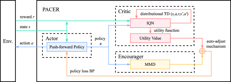
Figure 1: The structure of the PACER algorithm. The actor makes decisions according to a push-forward policy transformed from a basis distribution by DNNs. The critic models return distributions with quantile return representations and evaluating the policy via utility function on the return distribution. the encourager incentivizes exploration by guiding the actor to reduce the sample-based Maximum Mean Discrepancy between its policy and a reference policy.

Algorithm 1 PACER: Sample-based Distributional Actor-Critic-Encourager

1:environment $env$, replay buffer $\mathcal{B}$, initial policy networks $\theta_{\pi}$, quantile value networks $\theta_{z}$ and target networks $\hat{\theta}_{z}$.

2:Initialize parameters: number of quantiles K, batch size M, discounted factor $\gamma$, base distribution $\mathscr{P}(\xi)$, learning rate $\alpha_{z}$ and $\alpha_{\pi}$, MMD kernel $k$, MMD sample number $N_{m}$, utility function $\psi$.

3:for $n=1$ to $N$ do

4:     Sample a transition $\{(s_{n},a_{n},r_{n},s^{\prime}_{n})\}$ from $env$.

5:     $\mathcal{B}=\mathcal{B}\cup\{(s_{n},a_{n},r_{n},s^{\prime}_{n})\}$.

6:     if $\frac{n}{N_{update}}==0\ \&\ n\geq N_{explore}$ then

7:         Sample a batch $\mathcal{B}_{n}=\{(s_{m},a_{m},r_{m},s^{\prime}_{m})_{m=1}^{M}\}$ from $\mathcal{B}$.

8:         for each $(s_{m},a_{m},r_{m},s^{\prime}_{m})$ in $\mathcal{B}_{n}$ do

9:              $\triangleright$ Distributional TD learning.

10:              Generate quantiles $\{\tau_{i}\}_{i=1}^{K}$, $\{\tau_{j}\}_{j=1}^{K}$ and $\hat{\tau}_{i}=\frac{\tau_{i+1}+\tau_{i}}{2}$, $\hat{\tau}_{j}=\frac{\tau_{j+1}+\tau_{j}}{2}$.

11:              for $i=1$ to $K$, $j=1$ to $K$ do

12:                  $\delta_{ij}(s,a)=r(s,a)+\gamma z(s^{\prime},\pi(s^{\prime},\xi;\theta_{\pi}),\hat{\tau}_{i};\hat{\theta}_{z})-z(s,a,\hat{\tau}_{j};\theta_{z})$

13:              end for

14:              $\mathcal{L}^{m}(\theta_{z})=\sum_{i=1}^{K}\sum_{j=1}^{K}\rho_{\hat{\tau}_{i}}^{\kappa}\big{(}\delta_{ij}(s,a)\big{)}$

15:              $\triangleright$ Calcualte the utility value function and MMD regularizer.

16:              for $i=1$ to $N_{m}$ do

17:                  sample $\{\xi_{i},\xi_{j}\}\sim P(\xi)$, $\{a_{i},a_{j}\}$ from a uniform random policy.

18:                  $x_{i}=\pi(s^{\prime},\xi_{i};\theta_{\pi})$,$x_{j}=\pi(s^{\prime},\xi_{j};\theta_{\pi})$.

19:              end for

20:              $d^{m}(\theta_{\pi})=[\frac{1}{N_{m}^{2}}\sum^{N_{m}}_{i,j=1}\big{(}k(x_{i},x_{j})+k(a_{i},a_{j})-2k(x_{i},a_{j})\big{)}]^{\frac{1}{2}}$

21:              $V^{m}_{\psi}(s^{\prime})=\sum_{i=1}^{K}(\tau_{i+1}-\tau_{i})\psi^{\prime}(\hat{\tau_{i}})z\big{(}s,\pi(s,\xi;\theta_{\pi}),\hat{\tau}_{i};\theta_{z}\big{)}$.

22:         end for

23:         $\triangleright$ Construct loss functions.

24:         $\mathcal{L}(\theta_{z})=\frac{1}{M}\sum_{m=1}^{M}\mathcal{L}^{m}(\theta_{z})$.

25:         $\mathcal{L}(\theta_{\pi})=\frac{1}{M}\sum_{m=1}^{M}(-V^{m}_{\psi}(s^{\prime})+\alpha d^{m}(\theta_{\pi}))$

26:         $\mathcal{L}(\alpha)=ln\alpha(\beta-\frac{1}{M}\sum_{m=1}^{M}d^{m}(\theta_{\pi}))$.

27:         $\mathcal{L}(\beta)=\frac{1}{2}\beta[sign(\alpha_{\max}-\alpha)+sign(\alpha_{\min}-\alpha)]$.

28:         Update $\theta_{z},\ \theta_{\pi},\ \alpha,\ \beta$ according their loss functions.

29:     end if

30:end for

31:return $\pi(s,\xi;\theta_{\pi})$

3.1.1 Actor with push-forward policy

The actor of PACER is a deep neural network which acts as a push-forward operator transforming from a base distribution $\mathscr{P}(\mathcal{X})\in\mathcal{M}(\mathbb{R}^{d})$, where $\xi\sim\mathscr{P}(\mathcal{X})$ and $\xi\in\mathbb{R}^{d}$, to the action space $\mathcal{A}$ at a given state $s$ in a sample-to-sample manner. That is, $a\sim\pi(\cdot|s;\theta_{\pi}):=\pi(s,\xi;\theta_{\pi})_{\sharp}\mathscr{P}(\xi)$, where $\theta_{\pi}$ are the parameters of the DNN, and $\pi(s,\xi;\theta_{\pi}):\mathcal{S}\times\mathbb{R}\rightarrow\mathcal{A}$. Practically, an action in state $s$ can be generated in a lightweight approach by first sampling $\xi\sim\mathscr{P}(\xi)$ and then transforming it with $\pi(s,\xi;\theta_{\pi})$. Note that this kind of push-forward distributions has been shown to have high expressiveness and modelling capability both in theory and practice[5, 19], and has been widely used in the machine learning literature to approximately generate samples for complex distributions [24, 13, 19, 34]. While it is easy to obtain sample from push-forward policies, it is generally intractable to obtain its density function explicitly.

3.1.2 Critic with quantile return representation

The critic uses an IQN to push forward a sample from uniform distribution $U(0,1)$ to the corresponding quantile values sampled from the return distribution. The return distribution approximation is maintained by the weighted mixture of N Diracs. Notes that there are two alternative ways, QRN [15] and FQF [48], to represent quantile returns. However, QRN is designed for discrete actions, thus preclude continuous control tasks from its application. FQF requires additional computational steps to update another network for fraction proposal, and although it can obtain benefits, the complexity it brings is not conductive to the understanding of this proposed algorithm.

To reshape the policy’s random reward $R(s,a)$, a nonlinear reward-reshape type utility function $\psi(\cdot)$ is adopted. Specifically, we leverage the implicit quantile distribution $Z_{\pi}(s,a,\tilde{\tau};\theta_{z})$ defined in (4) to model the random return, and update it according to (5). With $\psi(R(s,a))$, we define the state-action utility function as

$$Q_{\psi}^{\pi}(s,a):=\mathbb{E}_{a\sim\pi(\cdot|s),s_{t+1}\sim\mathscr{P}(\cdot|s_{t},a_{t})}\left[\sum_{t=0}^{\infty}\gamma^{t}\psi(R(s,a))|_{s_{0}=s,a_{0}=a}\right],$$ (7)

and state utility function as

$$V_{\psi}^{\pi}(s):=\mathbb{E}_{a\sim\pi(\cdot|s)}[Q_{\psi}^{\pi}(s,a)].$$ (8)

Accordingly, the utility Bellman function can be defined as

$$Q_{\psi}^{\pi}(s,a):=\mathbb{E}_{R}[\psi(R(s,a))]+\gamma\mathbb{E}_{s^{\prime}\sim\mathscr{P}(\cdot|s,a)}[V_{\psi}^{\pi}(s^{\prime})].$$ (9)

For a given policy $\pi$, the critic evaluate it with $\mathbb{E}_{s\in\mu_{0}}V_{\psi}^{\pi}(s)$.

Remark 2.

We can also adopt risk-measure type utility functions in PACER, e.g., the distorted expectation [4] defined as follows.

A distortion expectation  $\psi:[0,1]\rightarrow[0,1]$ is a non-decreasing continuous function with $\psi(0)=0$ and $\psi(1)=1$. The distorted expectation of a random variable $Z$ under distortion function $\psi$ is given by: $\int_{0}^{1}F_{Z}^{-1}(\tau)d\psi(\tau)$. The distorted expectation for the random return of a given policy is defined as $\mathbb{E}_{s\sim\mu_{0},a\sim\pi(\cdot|s)}\int_{0}^{1}F_{Z_{\pi}(s,a)}^{-1}(\tau)d\psi(\tau)$.

3.1.3 Encourager with sample-based metric

Previous study has provided evidence for enhancing exploration by incorporating diverse behaviors in policies [20]. Building upon this idea, the encourager is constructed with the Maximum Mean Discrepancy (MMD), which incentivizes exploration by reducing MMD between agent’s policy $\pi(\cdot|s;\theta_{\pi})$ and a reference policy with diverse actions.

Definition 2.

(Maximum Mean Discrepancy). Let $\mathcal{F}$ be a unit ball in a Reproducing Kernel Hilbert Space $\mathcal{H}$ defined on a compact metric space $\mathcal{X}$. Then the maximum mean discrepancy between two distributions $p$ and $q$ is

$$MMD(p,q):=\sup_{f\in\mathcal{F}}\big{(}\mathbb{E}_{x\sim p}[f(x)]-\mathbb{E}_{y\sim q}[f(y)]\big{)}.$$ (10)

Note that MMD has an approximation which solely requires the samples from the distributions and does not demand the density functions explicitly. Given $m$-samples $\{x_{1},...,x_{m}\}$ from $p$ and $n$-samples $\{y_{1},...y_{n}\}$ from $q$, the MMD between $p$ and $q$ is approximated by

$$D_{m}(p||q):= \left[\frac{1}{m^{2}}\sum^{m}_{i,j=1}k(x_{i},x_{j})+\frac{1}{n^{2}}\sum^{n}_{i,j=1}k(y_{i},y_{j})-\frac{2}{mn}\sum^{m,n}_{i,j=1}k(x_{i},y_{j})\right]^{\frac{1}{2}}.$$ (11)

Here, we choose the uniform policy $u(\cdot|s)$ on the action space $\mathcal{A}$ as the reference policy. This uniform policy is widely utilized in the RL literature to facilitate exploration of the environment [9, 45]. We denote the sample-based regualrizer of encourager as the following expected MMD between $\pi(\cdot|s;\theta_{\pi})$ and $u(\cdot|s)$ by $d_{m}(\theta_{\pi})$,

$$d_{m}(\theta_{\pi}):=\mathbb{E}_{s\sim d_{\mu_{0}}^{\pi}}D_{m}\big{(}\pi(\cdot|s;\theta_{\pi})||u(\cdot|s)\big{)}.$$ (12)

Therefore, the exploration capability of the policy $\pi(\cdot|s;\theta_{\pi})$ is inversely proportional to $d_{m}{\theta_{\pi}}$. In practical, Monte Carlo method can be used to estimate the expectation, and the samples of policy $\pi(\cdot|s;\theta_{\pi})$ are generated as described in Sec 3.1.1.

3.2 The Stochastic Utility Value Policy Gradient Theorem

Combining the aforementioned components together, we obtain the objective for the policy in PACER as

$$J_{\psi}\left(\theta_{\pi}\right)=\mathbb{E}_{s\sim\mu_{0}}V_{\psi}^{\pi_{\theta}}(s)-\alpha\mathbb{E}_{s\sim d_{\mu 0}^{\pi}}D_{m}(\pi(\cdot|s;\theta_{\pi})||u(\cdot|s)),$$ (13)

where $\alpha>0$ denotes the regularizer weight. By maximizing $J_{\psi}\left(\theta_{\pi}\right)$, the policy pursues a large expected utility and maintains exploring to reduce the MMD regularizer. Generally, the optimization process in PACER can be divided into two steps. We firstly leverage distributional TD learning to update the parameter of IQN in the critic. The loss function for IQN is defined as follows, and it can be efficiently optimized using SGD method.

$$\mathcal{L}(\theta_{z})=\mathbb{E}_{s\sim d_{\mu_{0}}^{\pi},a\sim\pi(s,\xi;\theta_{\pi})}\sum_{i=0}^{N-1}\sum_{j=0}^{N^{\prime}-1}\rho_{\hat{\tau}_{i}}^{\kappa}\big{(}\delta_{ij}(s,a)\big{)},$$ (14)

where $\rho_{\hat{\tau}_{i}}^{\kappa}\big{(}\delta_{ij}(s,a)\big{)}$ is defined as equation (5). Then, we optimize the parameters in the policy according to $J_{\psi}\left(\theta_{\pi}\right)$ by leveraging gradient ascent iteratively.

Note that the first part $\mathbb{E}_{s\sim\mu_{0}}V_{\psi}^{\pi_{\theta}}(s)=\mathbb{E}_{s\sim\mu_{0}}\mathbb{E}_{a\sim\pi(\cdot|s,\theta_{\pi})}[Q_{\psi}^{\pi_{\theta}}(s,a)]$ of $J_{\psi}\left(\theta_{\pi}\right)$ is non-oblivious, i.e., the randomness of $\pi_{\theta}$ affects both the choice of action $a\sim\pi(\cdot|s,\theta_{\pi})$ and the function $Q_{\psi}^{\pi_{\theta}}(s,a)$, whose gradient is generally difficult to calculate. When the density of $\pi_{\theta}$ is calculable, we can compute its gradient according to the Stochastic Policy Gradient theorem [22]. However, as it is intractable to access the density of a push-forward policy with complex DNNs, we propose a stochastic policy gradient theorem that can be approximated only based on the samples of a policy.

Theorem 1 (Stochastic Utility Value Policy Gradient).

For a push-forward policy $\pi(s,\xi;\theta_{\pi})$ and a differentiable utility function $\psi(\cdot)$, the policy gradient of the state utility function $\mathbb{E}_{s\sim\mu_{0}}V_{\psi}^{\pi_{\theta}}(s)$ is given by

$$\nabla_{\theta_{\pi}}\mathbb{E}_{s\sim\mu_{0}}V_{\psi}^{\pi_{\theta}}(s)=\mathbb{E}_{s\sim d_{\mu 0}^{\pi},\xi\sim\mathscr{P}(\xi)}\left[\nabla_{\theta_{\pi}}\pi\left(s,\xi;\theta_{\pi}\right)\cdot\nabla_{a}Q_{\psi}^{\pi_{\theta}}\left(s,a\right)|_{a=\pi(s,\xi;\theta_{\pi})}\right].$$ (15)

According to Theorem 1, it can be verified that the gradient of $J_{\psi}\left(\theta_{\pi}\right)$ is as follows.

$$\mathbb{E}_{s\sim d_{\mu 0}^{\pi},\xi\sim\mathscr{P}(\xi)}\nabla_{\theta_{\pi}}\left[\pi\left(s,\xi;\theta_{\pi}\right)\cdot\nabla_{a}Q_{\psi}^{\pi_{\theta}}\left(s,a\right)-\alpha D_{m}(\pi(\cdot|s;\theta_{\pi})||u(\cdot|s))\right],$$ (16)

whose Monte-Carlo approximation can be efficiently calculated with only action samples from $\pi_{\theta}$ and the push-forward map $\pi\left(s,\xi;\theta_{\pi}\right)$.

When a risk-measure type utility function, e.g., the distorted expectation, is used in PACER, we can let $\psi$ in SUVPG be the identity map. Then, we obtain a fully sample-based version of the Stochastic Policy Gradient (SPG). As a result, we can train our PACER algorithm just in the same way as the training process in DSAC for risk-measure type utility functions, by replacing the SPG estimator in DSAC with our sample-based one.

Actually, SUVPG can be regarded as the policy gradient obtained under the reparameterization trick [23], while the widely used REINFORCE gradient [22] is based on the log-derivative trick. This also suggests that SUVPG is applicable to a wide range of familiar policy gradient approaches, such as advantage variance-reduction [42] and natural gradient [2].

3.3 An Adaptive Weight-Adjustment Mechanism

Inspired by the automating temperature adjustment mechanism for Maximum Entropy RL [21], we implement an adaptive mechanism to automatically adjust the weight parameter $\alpha$ for the Encourager.

By considering the MMD regularizer as a constraint, we can reformulate $\max J_{\psi}\left(\theta_{\pi}\right)$ as the following constrained optimization problem:

$$\max_{\theta_{\pi}} \ \mathbb{E}_{s\sim\mu_{0},\xi\sim\mathscr{P}(\xi)}\int_{0}^{1}F_{Z(s,\pi(s,\xi;\theta_{\pi}))}^{-1}(\tau)d\psi(\tau),$$ (17)

$$s.t. d_{m}(\theta_{\pi})\leq\beta.$$

Using Lagrange multipliers, the optimization problem can be converted into

$$\max_{\theta_{\pi}}\min_{\alpha\geq 0}f(\theta_{\pi},\alpha)\mathbb{E}_{s\sim\mu_{0},\xi\sim\mathscr{P}(\xi)}\int_{0}^{1}F_{Z(s,\pi(s,\xi;\theta_{\pi}))}^{-1}(\tau)d\psi(\tau)+\alpha(\beta-d_{m}(\theta_{\pi})).$$

The above problem can be optimized by iteratively solving the following two sub-problems: $max_{\theta_{\pi}}J_{\psi}\left(\theta_{\pi}\right)$ and $min_{\alpha\geq 0}\mathcal{L}(\alpha)$, in which

$$J_{\psi}\left(\theta_{\pi}\right) =\mathbb{E}_{s\sim\mu_{0},\xi\sim\mathscr{P}(\xi)}\int_{0}^{1}F_{Z(s,\pi(s,\xi;\theta_{\pi}))}^{-1}(\tau)d\psi(\tau)-\alpha d_{m}(\theta_{\pi}),\ \textrm{and}$$ (18)

$$\mathcal{L}(\alpha) =\alpha(\beta-d_{m}(\theta_{\pi})).$$

The constraint $d_{m}(\theta_{\pi})\leq\beta$ restricts the feasible policy space within the realm of the reference policy. Yet, the optimal $\beta$ could be varied from different training environments, which still needs manual tuning. Actually, an unsuitable $\beta$ would greatly deteriorate the performance of the algorithm.

Accordingly, we implement a new mechanism to adaptively obtain a trade-off between $\alpha$ and $\beta$, thus achieving a better balance between exploration and exploitation. Intuitively, the policy should progressively acquire knowledge during training, leading to a gradual increase in the impact of exploration. When $\beta$ is fixed, $\alpha$ will increase to counter the rising trend of Encourager during training. A high $\alpha$ indicates that the current training period requires a larger $\beta$ value, prompting the policy to increase its exploitation rate. Conversely, a low $\alpha$ suggests that the current training period has an excessive $\beta$ value, prompting the policy to enhance exploration by decreasing $\beta$. Thus, we define the following objective for $\beta$

$$\mathcal{L}(\beta)=\beta[\mathrm{sign}(\alpha_{\max}-\alpha)+\mathrm{sign}(\alpha_{\min}-\alpha)].$$ (19)

The parameters $\alpha_{\max}$ and $\alpha_{\min}$ that are suitable to PACER, can be set over a wide range, making them easy to configure practically.

4 Experiments

A comprehensive set of experiments are conducted to demonstrate the performance of PACER on MuJoCo continuous control benchmarks. The first is the comparison between PACER and other SOTA reinforcement learning algorithms. Our baselines include: Implicit Distributional Actor Critic (IDAC) [49] (the DRL algorithm leveraging Mixture of Gaussian policy), Distributional Soft Actor Critic (DSAC) [29] (a distributional version of SAC using quantile regression), as well as popular RL algorithms, DDPG [27], SAC [21], and TD3 [18]. For the baselines, we modified the code provided by SpinningUp [1] to implement SAC, DDPG, TD3, and we use the code from the websites provided in the original papers for IDAC and DSAC [49, 29]. The second experiment is the evaluation on the exploration capability of the push-forward policy. Moreover, ablation study is conducted to evaluate the effect of the push-forward policy and the MMD regularizer. At last, we also test the performance of PACER with different levels of CVaR utility function.

4.1 Settings

As suggested in [49, 29], we incorporates twin delayed networks and target networks in all the algorithms. In all the experiments except for the last one, the neutral utility function, i.e. identity map, are adopted in all the DRL algorithms for a fair comparison.

We fix batch size and total environment interactions for all the algorithms, and other tunable hyperparameters in different algorithms are either set to their best values according their original papers (if provided) or tuned with grid search on proper intervals. We list the key hyperparameters of PACER in appendix.

All experiments are conducted on Nvidia GeForce RTX 2080 Ti graphics cards, aiming to eliminate the performance variations caused by discrepancies in computing power. We train 5 different runs of each algorithm with 5 different random seeds. The evaluations are performed every 50 steps by calculating their averaged return. The total environment interactions are set to 1 millions and update the model parameters after collecting every 50 new samples.

4.2 Experimental results

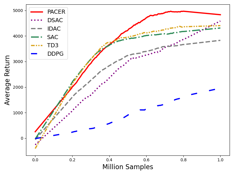
(a) Walker2d

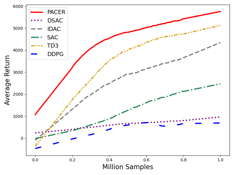
(b) Ant

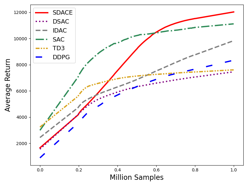
(c) HalfCheetah

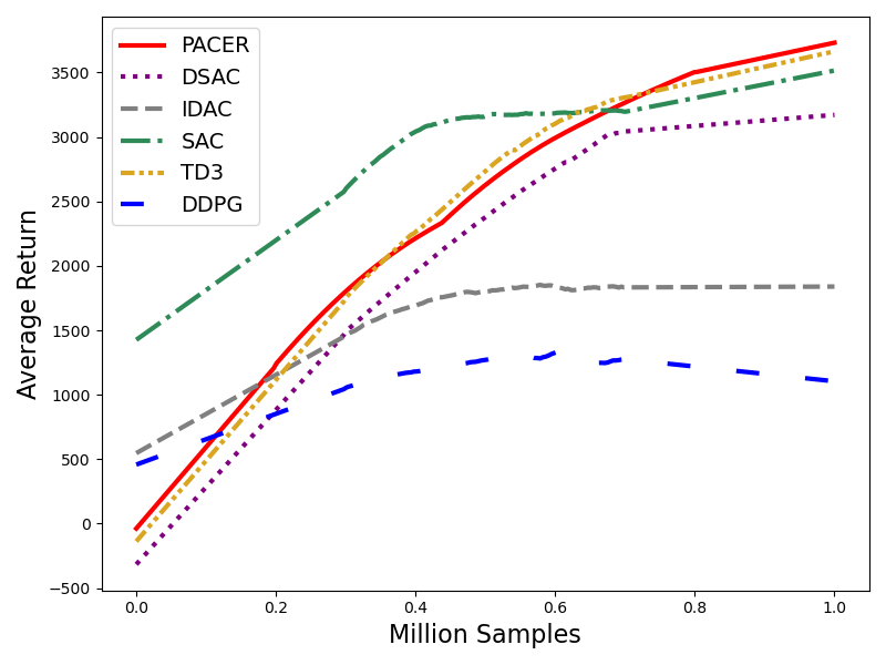
(d) Hopper

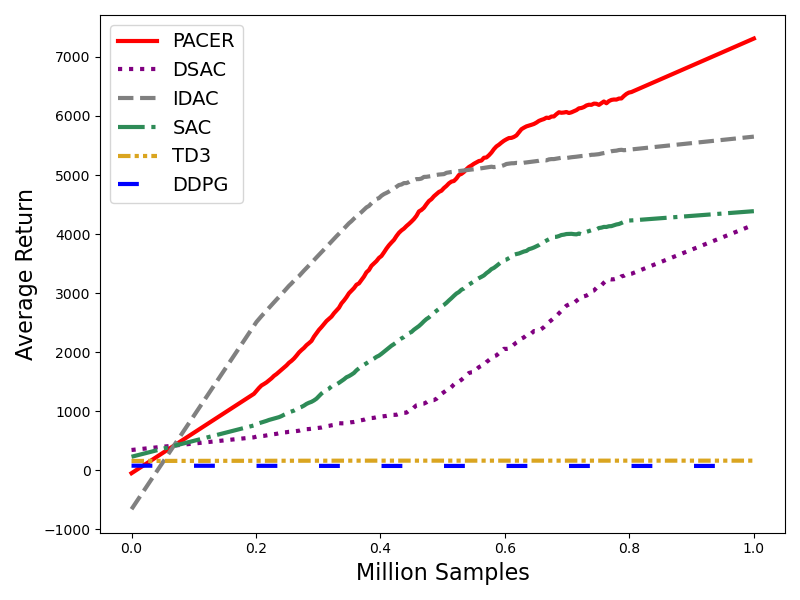
(e) Humanoid

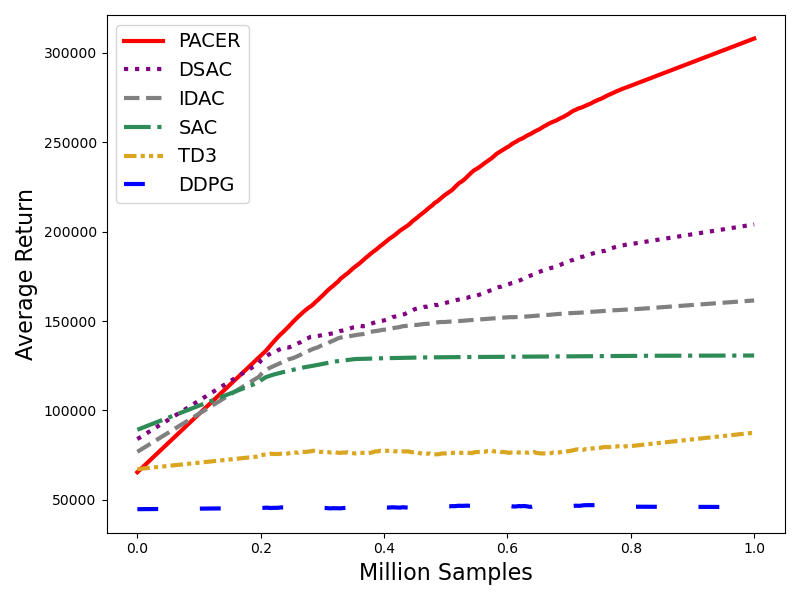
(f) Humanstandup

Figure 2: The training curves of PACER and baselines in MuJoCo continuous control tasks. All curves are smoothed with a window of length 100

Performance compared to SOTA. The learning curves are shown in figure 2 and the average final returns are listed in table 1. It can be observed that the proposed PACER algorithm outperforms all other algorithms across all benchmark tasks. Particularly, PACER can handle complex tasks (whose state and action dimensions are relative larger than other environments) effectively, where it gains $53.25\%$ improvements over HumanoidStandup and $59.72\%$ improvements over Humanoid tasks, compared to the existing SOTA. Additionally, the total score for DRL algorithms (PACER, IDAC, DSAC) are higher than the total score for Non-DRL algorithms (SAC, TD3, DDPG), which further demonstrates the advantage of modeling return distributions.

Table 1: Average final return (the maximum value for each task is bolded)

	Ant	Walker2d	Humanstandup	Humanoid	HalfCheetah	Hopper
PACER	5997.34	6213.28	312405.75	9257.93	12040.35	3588.56
IDAC	5154.094	3979.12	160750.56	5790.26	9788.23	3294.33
DSAC	1319.28	4605.83	203849.30	5400.88	7531.44	3132.13
SAC	3288.58	4455.96	130779.38	5161.05	11538.5	3536.81
TD3	5557.73	5118.61	114515.03	167.95	7705.37	3584.76
DDPG	2479.05	3672.8	68798.52	123.12	8434.51	2724.01

Exploration capability for Push-forward policy. We visualize the stochastic policies at the 10000th step of PACER on the Humanstandup task in Fig. 3. We focus on this task as it is the most complex task among all benchmarks. Specifically, we sample 100000 actions from the push-forward policy in a given state and create a heat maps on the (1,2) (9,10) and (14,15) dimensions over the total 17 dimension, respectively. It can be observed that the push-forward policy shows sufficient exploration ability even in the midst of the PACER training (10000th over the 20000 total steps) and would not degenerate into a deterministic policy.

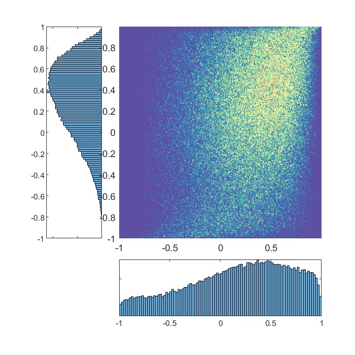
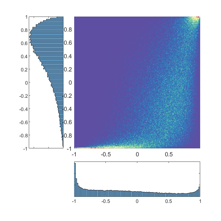
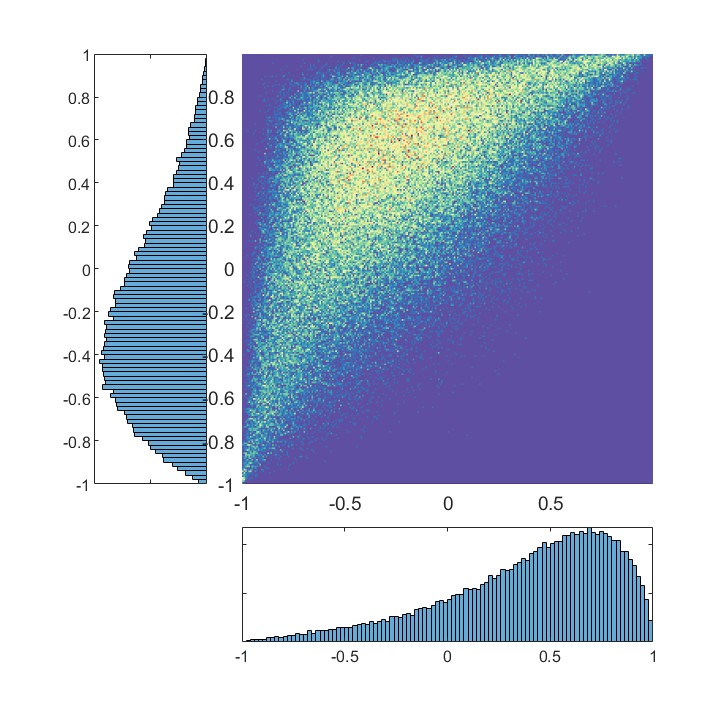
Figure 3: Visualization of the push-forward policies. In each sub-figure, the two distributions are formulated with 100000 sampled actions for one state that randomly selected in the training period, and the heat map is constructed by treating those distributions as the X-axis and Y-axis.

Ablation studies: significance and effect for each component. In Fig. 4(a), we shows the training curves of PACER, DSAC, IDAC and the ablated DRL algorithms derived from PACER on HumanoidStandup task. Detailed information of each algorithm is shown in table 2. The results exhibit the significance and effect of adopting push-forward policies and leveraging the MMD regularizer in continuous control tasks. We can see PACER, which leverages both MMD regularizer (M1) and push-forward policy (P1), outperforms all ablated algorithms that leverage one/none of the push-forward policy and MMD regularizer. Besides, the results also reveal that: (i) The MMD regularizer is also suitable to enhance exploration for the Guassian type policies as M1P0 achieves the next highest score. (ii) The absence of these crucial components significantly increases the probability of low performance or even failure. These findings offer compelling evidence for the effectiveness and significance of incorporating the push-forward policy and MMD regularizer within DRL algorithms.

Table 2: Ablation results

	Policy	Exploration	Frame	Score
PACER	push-forward	MMD	ACE	312405.75
M1P0	Gaussian	MMD	ACE	270045.92
M0P1G	push-forward	$\epsilon\ greedy$	AC	157777.47
M0P1	push-forward	None	AC	167379.97
M0P0G	Gaussian	$\epsilon\ greedy$	AC	165686.65
M0P0	Gaussian	None	AC	161008.71
DSAC	Gaussian	entropy	SAC	203849.30
IDAC	Gaussian	entropy	SAC	160750.56

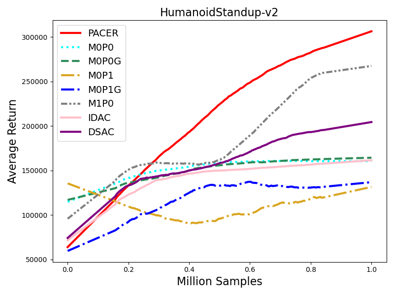
(a) Ablation

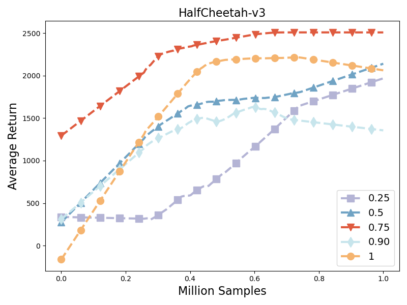
(b) Utility function

Figure 4: (a) Ablation experiments result, where we denote the push-forward policy with P, the MMD regularizer with M, and $P0$, $M0$ represent the PACER-induced algorithm without the corresponding techniques. (b) The results for different levels of CVaR under the modified HalfCheetah environment.

Effectiveness for Utility function. In this part, we follow the same idea as [3] to show the performance of PACER with different levels of CVaR utility function. Specifically, we modify the reward function in the HalfCheetah task as $R_{t}(s,a)=\bar{r}_{t}(s,a)-70\mathbb{I}_{v>4}\cdot\mathcal{B}_{0.1}$, where $R_{t}(s,a)$ is the modified reward, $\bar{r}_{t}(s,a)$ is the original reward, and $v$ is the forward velocity. This modification will penalize high velocities ($v>4$) with a Bernoulli distribution ($\mathcal{B}_{0.1}$), which represents rare but catastrophic events. We leverage CVaR with level $={0.25,0.5,0.75,0.90,1}$ as our utility functions. The results are shown in Fig. 4(b). It is evident that the policy with a 0.75-CVaR outperforms the risk-neutral policy (1-CVaR), since the actor employing the 0.75-CVaR policy demonstrates risk aversion towards the infrequent yet catastrophic event that robot breakdowns. The result shows that PACER with proper utility functions has the ability to obtain risk-sensitive policies.

5 Conclusions

We present PACER in this paper, the first fully push-forward-based Distributional Reinforcement Learning algorithm. We simultaneously leverage the push-forward operator to model return distributions and stochastic policies, enabling them with equal modeling capability and enhancing synergetic performance. The compatible with the push-forward policies in PACER, a sample-based exploration-induced regularizer and a stochastic utility value policy gradient theorem are established. We validate the critical roles of components in our algorithm with a detailed ablation study, and demonstrate that our algorithm is capable of handling state-of-the-art performance on a number of challenging continuous control problems.

Appendix

Proof for Theorem 1.

Theorem (Stochastic Utility Value Policy Gradient).

The gradient of the target function $J_{\psi}\left(\theta_{\pi}\right)=\mathbb{E}_{s\sim\mu_{0}}V_{\psi}^{\pi_{\theta}}(s)$ is given by

$$\mathbb{E}_{s\sim d_{\mu 0}^{\pi},\xi\sim\mathscr{P}(\xi)}\left[\nabla_{\theta_{\pi}}\pi\left(s,\xi;\theta_{\pi}\right)\cdot\nabla_{a}Q_{\psi}^{\pi_{\theta}}\left(s,a\right)|_{a=\pi(s,\xi;\theta_{\pi})}\right].$$ (20)

Proof.

According to the definition of $J_{\psi}\left(\theta_{\pi}\right)$, its gradient can be written as

$$\nabla_{\theta_{\pi}}J_{\psi}(\theta_{\pi})=\nabla_{\theta_{\pi}}\mathbb{E}_{s\sim\mu_{0}}V_{\psi}^{\pi_{\theta}}(s)=\int_{\mathcal{S}}\mu_{0}(s)\nabla_{\theta_{\pi}}V_{\psi}^{\pi_{\theta}}(s)\mathrm{d}s.$$ (21)

Thus we focus on the gradient of $V_{\psi}^{\pi_{\theta}}(s)$.

$$\nabla_{\theta_{\pi}}V_{\psi}^{\pi_{\theta}}(s)=\nabla_{\theta_{\pi}}\int_{\mathcal{X}}\mathscr{P}(\xi)Q_{\psi}^{\pi_{\theta}}\left(s,\pi\left(s,\xi;\theta_{\pi}\right)\right)\mathrm{d}\xi=\int_{\mathcal{X}}\mathscr{P}(\xi)\nabla_{\theta_{\pi}}Q_{\psi}^{\pi_{\theta}}\left(s,\pi\left(s,\xi;\theta_{\pi}\right)\right)\mathrm{d}\xi,$$ (22)

where the gradient of $Q_{\psi}^{\pi_{\theta}}\left(s,\pi\left(s,\xi;\theta_{\pi}\right)\right)$ can be calculated by,

$$\nabla_{\theta_{\pi}}Q_{\psi}^{\pi_{\theta}}\left(s,\pi\left(s,\xi;\theta_{\pi}\right)\right)$$

$$=\nabla_{\theta_{\pi}}[\psi\big{(}R(s,\pi\left(s,\xi;\theta_{\pi}\right))\big{)}+\gamma\mathbb{E}_{s^{\prime}\sim\mathscr{P}(\cdot|s,\pi\left(s,\xi;\theta_{\pi}\right))}V_{\psi}^{\pi_{\theta}}(s^{\prime})]$$

$$=\nabla_{\theta_{\pi}}\psi\big{(}R(s,\pi\left(s,\xi;\theta_{\pi}\right))\big{)}+\gamma\nabla_{\theta_{\pi}}\int_{\mathcal{S}}\mathscr{P}(s^{\prime}|s,\pi\left(s,\xi;\theta_{\pi}\right))V_{\psi}^{\pi_{\theta}}(s^{\prime})\mathrm{d}s^{\prime}$$

$$=\nabla_{\theta_{\pi}}\pi\left(s,\xi;\theta_{\pi}\right)\nabla_{a}\psi\big{(}R(s,a)\big{)}|_{a=\pi(s,\xi;\theta_{\pi})}$$

$$\ \ +\int_{\mathcal{S}}\gamma\nabla_{\theta_{\pi}}\pi\left(s,\xi;\theta_{\pi}\right)\nabla_{a}\mathscr{P}(s^{\prime}|s,\pi\left(s,\xi;\theta_{\pi}\right))|_{a=\pi(s,\xi;\theta_{\pi})}V_{\psi}^{\pi_{\theta}}(s^{\prime})\mathrm{d}s^{\prime}$$

$$\ \ +\int_{\mathcal{S}}\gamma\mathscr{P}(s^{\prime}|s,\pi\left(s,\xi;\theta_{\pi}\right))\nabla_{\theta_{\pi}}V_{\psi}^{\pi_{\theta}}(s^{\prime})\mathrm{d}s^{\prime}$$

$$=\nabla_{\theta_{\pi}}\pi\left(s,\xi;\theta_{\pi}\right)\nabla_{a}[\psi\big{(}R(s,a)\big{)}+\int_{\mathcal{S}}\gamma\mathscr{P}(s^{\prime}|s,\pi\left(s,\xi;\theta_{\pi}\right))V_{\psi}^{\pi_{\theta}}(s^{\prime})\mathrm{d}s^{\prime}]|_{a=\pi(s,\xi;\theta_{\pi})}$$

$$\ \ +\int_{\mathcal{S}}\gamma\mathscr{P}(s^{\prime}|s,\pi\left(s,\xi;\theta_{\pi}\right))\nabla_{\theta_{\pi}}V_{\psi}^{\pi_{\theta}}(s^{\prime})\mathrm{d}s^{\prime}$$

$$=\nabla_{\theta_{\pi}}\pi\left(s,\xi;\theta_{\pi}\right)\nabla_{a}Q_{\psi}^{\pi_{\theta}}(s,a)|_{a=\pi(s,\xi;\theta_{\pi})}+\int_{\mathcal{S}}\gamma\mathscr{P}(s^{\prime}|s,\pi\left(s,\xi;\theta_{\pi}\right))\nabla_{\theta_{\pi}}V_{\psi}^{\pi_{\theta}}(s^{\prime})\mathrm{d}s^{\prime}.$$

By substituting this back into (22), we have

$$\nabla_{\theta_{\pi}}V_{\psi}^{\pi_{\theta}}(s) =\int_{\mathcal{X}}\mathscr{P}(\xi)\nabla_{\theta_{\pi}}\pi\left(s,\xi;\theta_{\pi}\right)\nabla_{a}Q_{\psi}^{\pi_{\theta}}(s,a)|_{a=\pi(s,\xi;\theta_{\pi})}\mathrm{d}\xi$$

$$\ \ +\int_{\mathcal{X}}\mathscr{P}(\xi)\int_{\mathcal{S}}\gamma\mathscr{P}(s\rightarrow s^{\prime},1,\pi_{\theta})\nabla_{\theta_{\pi}}V_{\psi}^{\pi_{\theta}}(s^{\prime})\mathrm{d}s^{\prime}\mathrm{d}\xi,$$

where $\mathscr{P}(s\rightarrow s^{\prime},1,\pi_{\theta})$ indicates the probability that $s$ transforms to $s^{\prime}$ in one step with policy $\pi_{\theta}$. We can see that $\nabla_{\theta_{\pi}}V^{\pi_{\theta}}(s)$ have an iteration property, thus we can obtain that $\nabla_{\theta_{\pi}}V_{\psi}^{\pi_{\theta}}$ equals to

$$\mathbb{E}_{\xi\sim\mathscr{P}(\xi)}\int_{\mathcal{S}}\sum_{t=0}^{\infty}\gamma^{t}\mathscr{P}(s\rightarrow s^{\prime},t,\pi_{\theta})\nabla_{\theta_{\pi}}\pi(s^{\prime},\xi^{\prime};\theta_{\pi})\nabla_{a^{\prime}}Q_{\psi}^{\pi_{\theta}}(s^{\prime},a^{\prime})|_{a^{\prime}=\pi(s^{\prime},\xi^{\prime};\theta_{\pi})}\mathrm{d}s^{\prime}.$$

As a result, we can conclude that $\nabla_{\theta_{\pi}}J_{\psi}(\theta_{\pi})$

$$=\int_{\mathcal{S}}\mu_{0}(s)\mathbb{E}_{\xi\sim\mathscr{P}(\xi)}\int_{\mathcal{S}}\sum_{t=0}^{\infty}\gamma^{t}\mathscr{P}(s\rightarrow s^{\prime},t,\pi_{\theta})\nabla_{\theta_{\pi}}\pi(s^{\prime},\xi^{\prime};\theta_{\pi})\nabla_{a^{\prime}}Q_{\psi}^{\pi_{\theta}}(s^{\prime},a^{\prime})|_{a^{\prime}=\pi(s^{\prime},\xi^{\prime};\theta_{\pi})}\mathrm{d}s^{\prime}\mathrm{d}s$$

$$=\mathbb{E}_{s\sim d_{\mu 0}^{\pi},\xi\sim\mathscr{P}(\xi)}\left[\nabla_{\theta_{\pi}}\pi\left(s,\xi;\theta_{\pi}\right)\cdot\nabla_{a}Q_{\psi}^{\pi_{\theta}}\left(s,a\right)|_{a=\pi(s,\xi;\theta_{\pi})}\right]$$

∎

Implementation Details

We use the following techniques in Mujoco environments for training stability, all of them are also applied to baseline algorithms for fair comparisons.

• Observation Normalization: in mujoco environments, the observation ranges from $-\infty$ to $\infty$. We normalize the observations by $clip\big{(}(s-\hat{\mu}_{s})/(\max(\hat{\sigma}_{s})),-5,5\big{)}$, where $\hat{\mu}_{s}$ is the mean of observations and $\hat{\sigma}_{s}$ is the standard deviation of observations.

• Reward Scaling: the reward signal for the environment HumanoidStandup is too large, so we shrink it for numerical stability. Notice that the change only reacts on training period, all testing experiments are carried out on the same reward signals.

Table 3: Hyper-parameters settings

Hyper-parameters	Value
$q_{train}(z)$	$\mathcal{N}(0,1)$
$q_{test}(z)$	$\mathcal{N}(0,0.5)$
Number of quantiles	$32$
Policy network learning rate	$1\times 10^{-3}$
(Quantile) Value network learning rate	$1\times 10^{-3}$
Optimizer	Adam
Replay Buffer Size	$10^{6}$
Total environment interactions	$1\times 10^{6}$
Batch Size	$100$
Number of training steps per update	$50$
MMD sample numbers $m$	$100$
$\lambda$	$0.99$
The step of $\beta$	$0.01$

Table 4: Network Structure

Actor	Critic
(state dim + epsilon dim, 400)	(state dim + act dim, 400)
Relu	Relu
(400, 300)	(400, 300)
Relu	Relu
(300, action dim)	(300, 1)
Tanh

References

- \bibcommenthead
- Achiam [2018] Achiam J (2018) Spinning Up in Deep Reinforcement Learning
- Amari [1998] Amari SI (1998) Natural gradient works efficiently in learning. Neural computation 10(2):251–276
- Armengol Urpí et al [2021] Armengol Urpí N, Curi S, Krause A (2021) Risk-averse offline reinforcement learning. In: ICLR 2021, OpenReview
- Balbás et al [2009] Balbás A, Garrido J, Mayoral S (2009) Properties of distortion risk measures. Methodology and Computing in Applied Probability 11(3):385–399
- Baptista et al [2023] Baptista R, Hosseini B, Kovachki NB, et al (2023) An approximation theory framework for measure-transport sampling algorithms. arXiv preprint arXiv:230213965
- Barth-Maron et al [2018] Barth-Maron G, Hoffman MW, Budden D, et al (2018) Distributed distributional deterministic policy gradients. In: ICLR 2018
- Bellemare et al [2017] Bellemare MG, Dabney W, Munos R (2017) A distributional perspective on reinforcement learning. In: ICML 2017, PMLR, pp 449–458
- Bellemare et al [2023] Bellemare MG, Dabney W, Rowland M (2023) Distributional Reinforcement Learning. MIT Press, http://www.distributional-rl.org
- Burda et al [2019] Burda Y, Edwards H, Storkey A, et al (2019) Exploration by random network distillation. In: Seventh International Conference on Learning Representations, pp 1–17
- Choi et al [2021] Choi J, Dance C, Kim Je, et al (2021) Risk-conditioned distributional soft actor-critic for risk-sensitive navigation. In: ICRA 2021, IEEE, pp 8337–8344
- Chow et al [2015] Chow Y, Tamar A, Mannor S, et al (2015) Risk-sensitive and robust decision-making: a cvar optimization approach. Advances in neural information processing systems 28
- Chow et al [2017] Chow Y, Ghavamzadeh M, Janson L, et al (2017) Risk-constrained reinforcement learning with percentile risk criteria. J Mach Learn Res 18(1):6070–6120
- Creswell et al [2018] Creswell A, White T, Dumoulin V, et al (2018) Generative adversarial networks: An overview. IEEE signal processing magazine 35(1):53–65
- Dabney et al [2018a] Dabney W, Ostrovski G, Silver D, et al (2018a) Implicit quantile networks for distributional reinforcement learning. In: ICML 2018, PMLR, pp 1096–1105
- Dabney et al [2018b] Dabney W, Rowland M, Bellemare M, et al (2018b) Distributional reinforcement learning with quantile regression. In: AAAI 2018
- Duan et al [2021] Duan J, Guan Y, Li SE, et al (2021) Distributional soft actor-critic: Off-policy reinforcement learning for addressing value estimation errors. IEEE transactions on neural networks and learning systems
- Engel et al [2005] Engel Y, Mannor S, Meir R (2005) Reinforcement learning with gaussian processes. In: Proceedings of the 22nd international conference on Machine learning, pp 201–208
- Fujimoto et al [2018] Fujimoto S, Hoof H, Meger D (2018) Addressing function approximation error in actor-critic methods. In: ICML 2018, PMLR, pp 1587–1596
- Goodfellow et al [2020] Goodfellow I, Pouget-Abadie J, Mirza M, et al (2020) Generative adversarial networks. Communications of the ACM 63(11):139–144
- Haarnoja et al [2017] Haarnoja T, Tang H, Abbeel P, et al (2017) Reinforcement learning with deep energy-based policies. In: ICML 2017, PMLR, pp 1352–1361
- Haarnoja et al [2018] Haarnoja T, Zhou A, Hartikainen K, et al (2018) Soft actor-critic algorithms and applications. arXiv preprint arXiv:181205905
- Heess et al [2015] Heess N, Wayne G, Silver D, et al (2015) Learning continuous control policies by stochastic value gradients. Advances in neural information processing systems 28
- Kingma and Welling [2013] Kingma DP, Welling M (2013) Auto-encoding variational bayes. arXiv preprint arXiv:13126114
- Kingma et al [2014] Kingma DP, Mohamed S, Jimenez Rezende D, et al (2014) Semi-supervised learning with deep generative models. NIPS 2014 27
- Konda and Tsitsiklis [1999] Konda V, Tsitsiklis J (1999) Actor-critic algorithms. Advances in neural information processing systems 12
- Kuznetsov et al [2020] Kuznetsov A, Shvechikov P, Grishin A, et al (2020) Controlling overestimation bias with truncated mixture of continuous distributional quantile critics. In: International Conference on Machine Learning, PMLR, pp 5556–5566
- Lillicrap et al [2015] Lillicrap TP, Hunt JJ, Pritzel A, et al (2015) Continuous control with deep reinforcement learning. arXiv preprint arXiv:150902971
- Lindenberg et al [2022] Lindenberg B, Nordqvist J, Lindahl KO (2022) Conjugated discrete distributions for distributional reinforcement learning. In: AAAI 2022, pp 7516–7524
- Ma et al [2020] Ma X, Xia L, Zhou Z, et al (2020) Dsac: distributional soft actor critic for risk-sensitive reinforcement learning. arXiv preprint arXiv:200414547
- Marzouk et al [2016] Marzouk Y, Moselhy T, Parno M, et al (2016) Sampling via measure transport: An introduction. Handbook of uncertainty quantification 1:2
- Mnih et al [2015] Mnih V, Kavukcuoglu K, Silver D, et al (2015) Human-level control through deep reinforcement learning. nature 518(7540):529–533
- MORIMURA [2010] MORIMURA T (2010) Parametric return density estimation for reinforcement learning. In: Conference on Uncertainty in Artificial Intelligence, 2010
- Nam et al [2021] Nam DW, Kim Y, Park CY (2021) Gmac: A distributional perspective on actor-critic framework. In: ICML 2021, PMLR, pp 7927–7936
- Ororbia and Kifer [2022] Ororbia A, Kifer D (2022) The neural coding framework for learning generative models. Nature communications 13(1):2064
- Parno and Marzouk [2018] Parno MD, Marzouk YM (2018) Transport map accelerated markov chain monte carlo. SIAM/ASA Journal on Uncertainty Quantification 6(2):645–682
- Peherstorfer and Marzouk [2019] Peherstorfer B, Marzouk Y (2019) A transport-based multifidelity preconditioner for markov chain monte carlo. Adv Comput Math 45:2321–2348
- Peyré et al [2019] Peyré G, Cuturi M, et al (2019) Computational optimal transport: With applications to data science. Found Trends Mach Learn 11(5-6):355–607
- Prashanth and Ghavamzadeh [2016] Prashanth L, Ghavamzadeh M (2016) Variance-constrained actor-critic algorithms for discounted and average reward mdps. Machine Learning 105(3):367–417
- Prashanth et al [2022] Prashanth L, Fu MC, et al (2022) Risk-sensitive reinforcement learning via policy gradient search. Found Trends Mach Learn 15(5):537–693
- Rowland et al [2018] Rowland M, Bellemare M, Dabney W, et al (2018) An analysis of categorical distributional reinforcement learning. In: AISTATS 2018, PMLR, pp 29–37
- Sato et al [2001] Sato M, Kimura H, Kobayashi S (2001) Td algorithm for the variance of return and mean-variance reinforcement learning. Trans Jpn Soc Artif 16(3):353–362
- Schulman et al [2015] Schulman J, Moritz P, Levine S, et al (2015) High-dimensional continuous control using generalized advantage estimation. arXiv preprint arXiv:150602438
- Singh et al [2020] Singh R, Zhang Q, Chen Y (2020) Improving robustness via risk averse distributional reinforcement learning. In: Learning for Dynamics and Control, pp 958–968
- Singh et al [2022] Singh R, Lee K, Chen Y (2022) Sample-based distributional policy gradient. In: Learning for Dynamics and Control Conference, PMLR, pp 676–688
- Sukhbaatar et al [2018] Sukhbaatar S, Lin Z, Kostrikov I, et al (2018) Intrinsic motivation and automatic curricula via asymmetric self-play. In: 6th International Conference on Learning Representations, ICLR 2018
- Sutton and Barto [2018] Sutton RS, Barto AG (2018) Reinforcement learning: An introduction. MIT press
- Villani et al [2009] Villani C, et al (2009) Optimal transport: old and new, vol 338. Springer
- Yang et al [2019] Yang D, Zhao L, Lin Z, et al (2019) Fully parameterized quantile function for distributional reinforcement learning. NeurIPS 2019 32
- Yue et al [2020] Yue Y, Wang Z, Zhou M (2020) Implicit distributional reinforcement learning. Advances in Neural Information Processing Systems 33:7135–7147
- Ziebart [2010] Ziebart BD (2010) Modeling purposeful adaptive behavior with the principle of maximum causal entropy. Carnegie Mellon University