Abstract

This paper extends continuous contraction theory of nonlinear dynamical systems to systems with nonlinear inequality constraints. It shows that the contraction behaviour of the constrained dynamics is given by the covariant derivative of the system dynamics from the original contraction theorem [5], plus the second covariant derivative of the active inequality constraint. It is shown that this approach works both for a step Lagrangian constraint term at a first-order system as well for a Dirac Lagrangian constraint term for a second-order system.

Practical applications include controllers constrained to an operational envelope, trajectory control with moving obstacles, and a classical Lagrangian interpretation of the single and two slit experiments of quantum mechanics.

1 Introduction

This paper extends contraction theory [5] of unconstrained $n$-dimensional nonlinear dynamics in covariant form,

$${\bf M}({\bf x},t)\ \dot{\bf x}={\bf f}({\bf x},t)$$ (1)

where ${\bf M}({\bf x},t)$ is a Riemannian metric, to systems with $j=1,...,J$-dimensional inequality constraints

$$g_{j}({\bf x},t)\leq 0$$ (2)

Note that the above ’covariant’ form [9] corresponds to the $n$-dimensional ’contravariant’ [9] dynamics

$$\dot{\bf x}\ =\ {\bf f}^{\prime}({\bf x},t)$$

with ${\bf f}={\bf M}{\bf f}^{\prime}$, which is used in the original contravariant contraction theorem [5]. This paper will use covariant coordinates since the constraint terms introduced later will be covariant. While both representations are fully equivalent, in this case covariant coordinates are simpler.

This paper computes continuous-time contraction rates in section 2.1 for ${\bf M}={\bf I}$ and in section 2.2 for a general metric ${\bf M}({\bf x},t)$. Finally the result is applied to second-order collsion dynamics in section 2.3. The discussion is illustrated with simple applications, including

• trajectory control considering moving obstacles as constraint

• second-order controller operation in a constrained operational envelope

• a Lagrangian collision interpretation of the single and double slit experiment of quantum mechanics

A discrete-time version of the approach is derived in [8], along with an application to piece-wise linear neuronal networks.

2 Continuous-time constrained dynamics

A constraint $j$ in equation (2) can have only an impact on the dynamics (1) if the inequality turns in an equality $g_{j}({\bf x},t)=0$ , leading to the following definition.

Definition 1

The set of active constraints $\mathcal{A}({\bf x},t)\subset\{1,...,J\}$ (2) contains the elements $j$ which are on the boundary of the original constraint

$$g_{j}({\bf x},t)=0$$

The constrained dynamic equations (1, 2) are then of the form [2]

$${\bf M}\dot{\bf x}={\bf f}({\bf x},t)+\sum_{all\ j\in\mathcal{A}}\frac{\partial g_{j}}{\partial{\bf x}}\lambda_{j}$$ (3)

All constraints $g_{j},j\in\mathcal{A}$ are not violated at $t+dt$ if [2]

$$\dot{g}_{j}=\frac{\partial{g}_{j}}{\partial{\bf x}}^{T}{\bf M}^{-1}\left({\bf f}({\bf x},t)+\sum_{all\ j\in\mathcal{A}}\frac{\partial g_{j}}{\partial{\bf x}}\lambda_{j}\right)+\frac{\partial{g}_{j}}{\partial t} \leq 0$$ (4)

leading to

Definition 2

The set of Lagrange multipliers $\lambda_{j},j\in\mathcal{A}({\bf x},t)$ of (2) are defined as

$$\lambda_{j} \leq -\sum_{k\in\mathcal{A}({\bf x},t)}\frac{\frac{\partial{g}_{k}}{\partial{\bf x}}^{T}{\bf M}^{-1}{\bf f}({\bf x},t)+\frac{\partial{g}_{k}}{\partial t}}{\frac{\partial{g}_{j}}{\partial{\bf x}}^{T}{\bf M}^{-1}\frac{\partial g_{k}}{\partial{\bf x}}}$$

where we assume without loss of generality

• that all corners are obtuse, i.e. $\frac{\partial{g}_{j}}{\partial{\bf x}}^{T}{\bf M}^{-1}\frac{\partial g_{k}}{\partial{\bf x}}({\bf x},t)\geq 0$ and

• that $\frac{1}{\frac{\partial{g}_{j}}{\partial{\bf x}}^{T}{\bf M}^{-1}\frac{\partial g_{k}}{\partial{\bf x}}}$ is replaced with the Moore-Penrose inverse [10] if $\frac{\partial{g}_{j}}{\partial{\bf x}}^{T}{\bf M}^{-1}\frac{\partial g_{k}}{\partial{\bf x}}$ does not have full rank.

Note that possible acute corners can be locally avoided by replacing the acute corner with two obtuse corners at the same ${\bf x},t$. Also note that alternatively the linear perogramming (LP) definition of [7] may be used.

Let us now introduce a virtual displacement between two neighbouring trajectories, constrained by $g_{j}({\bf x},t)=0$. This virtual displacement has to be parallel to $g_{j}({\bf x},t)=0$, i.e. orthogonal to the normals $\frac{\partial g_{j}}{\partial{\bf x}}$, which implies on the constraint

$${\bf\delta x} = {\bf G}_{\parallel}({\bf x},t)\ {\bf\delta x}^{\ast}$$

$${\bf G}_{\parallel}^{T}{\bf G}_{\parallel} = {\bf I}$$

$${\bf G}_{\parallel}^{T}\ \frac{\partial g_{j}}{\partial{\bf x}} = {\bf 0}\ \forall j\in\mathcal{A}({\bf x},t))$$ (5)

where ${\bf\delta x}^{\ast}$ is the reduced virtual displacement, which is of dimension $n$ minus the number of active constraints in $\mathcal{A}$. Note that all neighbouring trajectory steps $(\dot{\bf x}+\delta\dot{\bf x})dt$ around the main trajectory step $\dot{\bf x}dt$ arrive at the same time on the constraint since ($\delta\dot{\bf x}\ dt$) is a second-order term. Hence all neighbouring trajectories are constrained at the same time with (5).

The following two subsections analyse the contraction behaviour first for ${\bf M}={\bf I}$ and then for the general case.

2.1 Basic case

The constrained dynamic equations (3) can be rewritten for ${\bf M}={\bf I}$ as

$$\dot{\bf x}={\bf f}({\bf x},t)+\sum_{all\ j\in\mathcal{A}({\bf x},t)}\frac{\partial g_{j}}{\partial{\bf x}}\lambda_{j}={\bf f}({\bf x},t)+\sum_{j=1}^{J}\frac{\partial g_{j}}{\partial{\bf x}}step(g_{j})\lambda_{j}$$

with the Heaviside step function and Dirac impulse

$$\theta(g_{j}) = \left\{\begin{array}[]{l}0\text{\ \ for \ \ }g_{j}<0\\ 1\text{\ \ for \ \ }g_{j}=0\\ undefined\text{\ \ for \ \ }g_{j}>0\end{array}\right.$$ (9)

$$\delta(g_{j}) = \frac{\partial step(g_{j})}{\partial g_{j}}$$ (10)

whose variation is

$${\bf\delta\dot{x}}\ = \frac{\partial{\bf f}}{\partial{\bf x}}{\bf\delta x}+\sum_{j=1}^{J}\left(\left(\frac{\partial^{2}g_{j}}{\partial{\bf x}^{2}}\lambda_{j}+\frac{\partial g_{j}}{\partial{\bf x}}\frac{\partial\lambda_{j}}{\partial{\bf x}}^{T}\right)\theta(g_{j})+\frac{\partial g_{j}}{\partial{\bf x}}\delta(g_{j})\lambda_{j}\frac{\partial g_{j}}{\partial{\bf x}}^{T}\right){\bf\delta x}$$

Multiplying the above with $dt$ exactly at an activation of a constraint leads with $\lambda_{j}dt=\frac{dg_{j}}{\frac{\partial{g}_{j}}{\partial{\bf x}}^{T}\frac{\partial g_{j}}{\partial{\bf x}}}$ of Definition 2 to

$${\bf\delta{x}}_{t+dt}\ = \left({\bf I}-\sum_{allj\in\mathcal{A}}\frac{\frac{\partial g_{j}}{\partial{\bf x}}\frac{\partial g_{j}}{\partial{\bf x}}^{T}}{\frac{\partial{g}_{j}}{\partial{\bf x}}^{T}\frac{\partial g_{k}}{\partial{\bf x}}}\ \right){\bf\delta{x}}_{t}+dt\left(\frac{\partial{\bf f}}{\partial{\bf x}}+\sum_{allj\in\mathcal{A}}\left(\frac{\partial^{2}g_{j}}{\partial{\bf x}^{2}}\lambda_{j}+\frac{\partial g_{j}}{\partial{\bf x}}\frac{\partial\lambda_{j}^{T}}{\partial{\bf x}}\right)\right){\bf\delta x}$$

Performing the activation of the constraints sequentially (i.e. at least in infinitesimal time steps) we can see that the virtual displacement ${\bf\delta x}$ are set to ${\bf G}_{\parallel}{\bf\delta x}^{\ast}$ when a constraint is activated. The other terms can be neglected at the constraint activation since they are multiplied with $dt$. Now the squared virtual length dynamics can be computed outside the activation of a constraint as

$$\frac{1}{2}\ \frac{d}{dt}\left({\bf\delta x}^{T}{\bf\delta x}\right) = \ {\bf\delta x}^{\ast T}{\bf G}_{\parallel}^{T}\left(\frac{\partial{\bf f}}{\partial{\bf x}}+\sum_{allj\in\mathcal{A}}\frac{\partial^{2}g_{j}}{\partial{\bf x}^{2}}\lambda_{j}\right)_{H}{\bf G}_{\parallel}{\bf\delta x}^{\ast}$$

where we used ${\bf G}_{\parallel}^{T}\frac{\partial g_{j}}{\partial{\bf x}}\frac{\partial\lambda_{j}}{\partial{\bf x}}^{T}={\bf 0}$ since on the constraint the first two terms vanish and outside the constraint the last term vanishes.

Thus the dynamics of ${\bf\delta x}^{T}{\bf\delta x}$ is composed of exponentially convergent continuous segments and an enforcement of ${\bf\delta x}$ to ${\bf G}_{\parallel}{\bf\delta x}^{\ast}$ at the activation of a constraint.

2.2 More general metrics

We now extend the results of section 2.1 to a general metric ${\bf M}({\bf x},t)$, rather than identity. We recall the standard definition [9] of the covariant derivative operator $\nabla_{H}$ in a Riemann space with an underlying metric ${\bf M}({\bf x},t)$.

Definition 3

The covariant derivatives of a scalar $a({\bf x},t)$ or a vector ${\bf a}({\bf x},t)$ are defined as

$$\nabla_{M}\ a = \frac{\partial a}{\partial{\bf x}}\ =\ \nabla a$$

$$(\nabla_{M}\ {\bf a})_{ij} = \frac{\partial{\bf a}_{i}}{\partial{\bf x}_{j}}-\sum_{k=1}^{n}\gamma_{ij}^{k}\ {\bf a}_{k}$$

where $\ \gamma_{ij}^{k}\$ is the Christoffel term for the metric ${\bf M}({\bf x})$,

$$\gamma_{ij}^{k}({\bf x},t)=\frac{1}{2}\sum_{l=1}^{n}\left(\frac{\partial M_{il}}{\partial x^{j}}+\frac{\partial M_{jl}}{\partial x^{i}}-\frac{\partial M_{ij}}{\partial x^{l}}\right)M_{kl}^{-1}$$

The constrained dynamic equations (3) can be rewritten as

$${\bf M}\dot{\bf x}={\bf f}({\bf x},t)+\sum_{all\ j\in\mathcal{A}}\frac{\partial g_{j}}{\partial{\bf x}}\lambda_{j}={\bf f}({\bf x},t)+\sum_{j=1}^{J}\frac{\partial g_{j}}{\partial{\bf x}}step(g_{j})\lambda_{j}$$

whose variation is with (10)

$$\frac{\partial{\bf M}}{\partial{\bf x}}\ {\bf\delta x}\ \dot{\bf x}+{\bf M}{\bf\delta\dot{x}} = \frac{\partial{\bf f}}{\partial{\bf x}}{\bf\delta x}+\sum_{j=1}^{J}\left(\left(\frac{\partial^{2}g_{j}}{\partial{\bf x}^{2}}\lambda_{j}+\frac{\partial g_{j}}{\partial{\bf x}}\frac{\partial\lambda_{j}}{\partial{\bf x}}\right)\theta(g_{j})+\frac{\partial g_{j}}{\partial{\bf x}}\delta(g_{j})\lambda_{j}\frac{\partial g_{j}}{\partial{\bf x}}\right){\bf\delta x}$$

Multiplying the above with $dt$ exactly at an activation of a constraint leads with $\lambda_{j}dt=\frac{dg_{j}}{\frac{\partial{g}_{j}}{\partial{\bf x}}^{T}{\bf M}^{-1}\frac{\partial g_{j}}{\partial{\bf x}}}$ of Definition 2 to

$$\frac{\partial{\bf M}}{\partial{\bf x}}\ {\bf\delta x}\ \dot{\bf x}dt+{\bf M}{\bf\delta{x}}_{t+dt}$$

$$= \left({\bf M}-\sum_{allj\in\mathcal{A}}\frac{\frac{\partial g_{j}}{\partial{\bf x}}\frac{\partial g_{j}}{\partial{\bf x}}^{T}}{\frac{\partial{g}_{j}}{\partial{\bf x}}^{T}{\bf M}^{-1}\frac{\partial g_{j}}{\partial{\bf x}}}\ \right){\bf\delta{x}}_{t}+dt\left(\frac{\partial{\bf f}}{\partial{\bf x}}+\sum_{allj\in\mathcal{A}}\left(\frac{\partial^{2}g_{j}}{\partial{\bf x}^{2}}\lambda_{j}+\frac{\partial g_{j}}{\partial{\bf x}}\frac{\partial\lambda_{j}^{T}}{\partial{\bf x}}\right)\right){\bf\delta x}$$

Performing the activation of the constraints sequentially (i.e. at least in infinitesimal time steps) we can see that the virtual displacement ${\bf\delta x}$ are set to ${\bf G}_{\parallel}{\bf\delta x}^{\ast}$ when a constraint is activated. The other terms can be neglected at the constraint activation since they are multiplied with $dt$. Now the squared virtual length dynamics can be computed outside the activation of a constraint as

$$\frac{1}{2}\ \frac{d}{dt}\left({\bf\delta x}^{T}{\bf M}{\bf\delta x}\right) = \ {\bf\delta x}^{\ast T}{\bf G}_{\parallel}^{T}\left(\nabla_{M}\ {\bf f}+\frac{1}{2}\frac{\partial{\bf M}}{\partial t}+\sum_{all\ j\in\mathcal{A}}\lambda_{j}\nabla_{M}^{2}g_{j}\right)_{H}{\bf G}_{\parallel}{\bf\delta x}^{\ast}$$ (11)

where we used ${\bf G}_{\parallel}^{T}\frac{\partial g_{j}}{\partial{\bf x}}\frac{\partial\lambda_{j}}{\partial{\bf x}}={\bf 0}$ since on the constraint the first two terms vanish and outside the constraint the last term vanishes.

Thus the dynamics of ${\bf\delta x}^{T}{\bf\delta x}$ is composed of exponentially convergent continuous segments and an enforcement of ${\bf\delta x}$ to ${\bf G}_{\parallel}{\bf\delta x}^{\ast}$ at the activation of a constraint.

Summarizing the above leads to:

Theorem 1

Consider the continuous dynamics

$${\bf M}\dot{\bf x}={\bf f}({\bf x},t)+\sum_{all\ j\in\mathcal{A}}\lambda_{j}\frac{\partial g_{j}}{\partial{\bf x}}$$ (12)

within the metric ${\bf M}({\bf x},t)$ constrained by $j=1,...,J$ inequality constraints

$$g_{j}({\bf x},t)\leq 0$$

equivalent to the subset $\mathbb{G}^{n}\subset\mathbb{R}^{n}$. The set of active constraints $\mathcal{A}$ and Lagrange multipliers $\lambda_{j}$ are given in Definition 1 and 2.

The distance $s=\min\int_{{\bf x}(s)={\bf x}_{1}}^{{\bf x}_{2}}\sqrt{\delta{\bf x}^{T}{\bf M}\delta{\bf x}}$ within $\mathbb{G}^{n}$ from any trajectory ${\bf x}_{1}(t)$ to any other trajectory ${\bf x}_{2}(t)$ converges exponentially to $0$ with an exponential convergence rate $\leq\max_{along\ s}(\lambda_{\max}({\bf x},t)),\geq\min_{along\ s}(\lambda_{\min}({\bf x},t))$ with

$$\lambda_{\min}{\bf G}_{\parallel}^{T}{\bf M}{\bf G}_{\parallel}\leq{\bf G}_{\parallel}^{T}\left(\nabla_{M}\ {\bf f}+\frac{1}{2}\frac{\partial{\bf M}}{\partial t}+\sum_{all\ j\in\mathcal{A}}\lambda_{j}\nabla_{M}^{2}g_{j}\right)_{H}{\bf G}_{\parallel}\leq\lambda_{\max}{\bf G}_{\parallel}^{T}{\bf M}{\bf G}_{\parallel}$$ (13)

with the covariant derivative of Definition 3 and the constraint tangential space ${\bf G}_{\parallel}$ from equation (5).

In addition the activation of a constraint discontinuously sets the virtual displacement ${\bf\delta x}$ to ${\bf G}_{\parallel}{\bf\delta x}^{\ast}$.

Note that the inequality constraint in Theorem 13 can be replaced with an equality constraint if also the corresponding inequality in Definition 2 is replaced with an equality.

Also note that all lemmas of the original contraction theorem in [5] as adaptive control, observer design, combination principles etc. can be applied to Theorem 13 as well.

In addition note that [11] assessed the contraction behavior of nonlinear equality constraints. Initial principles for convex constraints and contraction theory were illustrated in [6, 12]. The following examples illustrate the application of Theorem 13 to different constrained dynamical systems:

• Example 2.1

  : Consider the inequality constraint in Figure 1

  $$g_{j}=x_{1}^{2}+x_{2}\leq 0$$

  

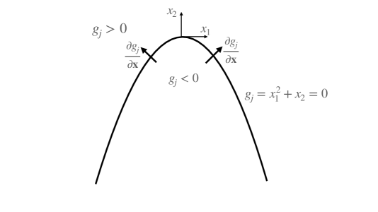
  Figure 1: Inequality constraint

  Regions of different signs of $g_{j}$ are shown in Figure 1, along with the gradient

  $$\frac{\partial g_{j}}{\partial{\bf x}}=\left(\begin{array}[]{c}2x_{1}\\ 1\end{array}\right)$$

  The constrained virtual displacement (5) is

  $${\bf\delta x}=\frac{1}{\sqrt{4x_{1}^{2}+1}}\left(\begin{array}[]{c}-1\\ 2x_{1}\end{array}\right)\delta x^{\ast}$$

  We consider now the divergent flow field

  $$\left(\begin{array}[]{c}\dot{x}_{1}\\ \dot{x}_{2}\end{array}\right)=\left(\begin{array}[]{c}x_{1}\\ x_{2}+1\end{array}\right)$$

  We compute the Lagrange multiplier of Definition 2 on the parabolic constraint $x_{1}^{2}=-x_{2}$ as

  $$\lambda_{j}\ = -\left(\frac{\partial g_{j}}{\partial{\bf x}}^{T}\frac{\partial g_{j}}{\partial{\bf x}}\right)^{-1}\left(\frac{\partial g_{j}}{\partial{\bf x}}^{T}{\bf f}+\frac{\partial g_{j}}{\partial t}\right)$$ (17)

  $$= -\frac{1}{4x_{1}^{2}+1}\left(\begin{array}[]{cc}2x_{1}&1\end{array}\right)\left(\begin{array}[]{c}x_{1}\\ x_{2}+1\end{array}\right)=-\frac{x_{1}^{2}+1}{4x_{1}^{2}+1}\leq 0$$

  I.e. the trajectories stay on the parabola once they moved on the parabola.

  We can bound with Theorem 13 the contraction behaviour (13) of the constrained dynamics (12)

  $$\frac{1}{2}\ \frac{d}{dt}\left({\bf\delta x}^{T}{\bf\delta x}\right) \leq {\bf\delta x}^{T}\left(\left(\begin{array}[]{cc}1&0\\ 0&1\end{array}\right)+\lambda_{j}\left(\begin{array}[]{cc}2&0\\ 0&0\end{array}\right)\right){\bf\delta x}$$ (22)

  The second term is only active on the 1-dimensional parabola $\mathcal{A}$ and decreases the divergence rate on the parabola. $\Box$

• Example 2.2

  : Consider a moving circular obstacle

  $$g_{j}=-(x_{1}-a(t))^{2}-(x_{2}-b(t))^{2}+1\leq 0$$

  The gradient at the constraint is

  $$\frac{\partial g_{j}}{\partial{\bf x}}=-2\left(\begin{array}[]{c}x_{1}-a\\ x_{2}-b\end{array}\right)$$

  The constrained virtual displacement (5) is hence

  $${\bf\delta x}=\frac{1}{\sqrt{(x_{1}-a)^{2}+(x_{2}-b)^{2}}}\left(\begin{array}[]{c}x_{2}-b\\ -(x_{1}-a)\end{array}\right)\delta x^{\ast}$$

  We consider now a robot which moves according to the convergent flow field

  $$\left(\begin{array}[]{c}\dot{x}_{1}\\ \dot{x}_{2}\end{array}\right)=-\left(\begin{array}[]{c}x_{1}\\ x_{2}\end{array}\right)$$

  We compute the Lagrange multiplier of Definition 2 on the circular constraint $(x_{1}-a)^{2}+(x_{2}-b)^{2}=1$ as

  $$\lambda_{j} = \min\left(-\left(\frac{\partial g_{j}}{\partial{\bf x}}^{T}\frac{\partial g_{j}}{\partial{\bf x}}\right)^{-1}\left(\frac{\partial g_{j}}{\partial{\bf x}}^{T}{\bf f}+\frac{\partial g_{j}}{\partial t}\right),0\right)$$ (26)

  $$= \min\left(-\frac{1}{2}\frac{1}{(x_{1}-a)^{2}+(x_{2}-b)^{2}}\left(\begin{array}[]{cc}x_{1}-a&x_{2}-b\end{array}\right)\left(\begin{array}[]{c}x_{1}+\dot{a}\\ x_{2}+\dot{b}\end{array}\right),0\right)$$

  We can upper and low bound with Theorem 13 the contraction behaviour (13) of the constrained dynamics (12) as

  $$\frac{1}{2}\ \frac{d}{dt}\left({\bf\delta x}^{T}{\bf\delta x}\right)=-(1+2\lambda_{j})\ {\bf\delta x}^{T}{\bf\delta x}$$

  The flow is globally contracting with $-(1+2\lambda_{j})$. Neighbouring trajectories exponentially converge with $e^{-\int(1+2\lambda_{j})dt}$.

  Figure 2 shows such a moving circle with velocity $v=\sqrt{\dot{a}^{2}+\dot{b}^{2}}$. The blue flow field is the unconstrained dynamics. The red flow is the Lagrangian normalisation and the black flow field, from which the contraction behaviour is computed in (13), is the flow on the constraint. $\Box$

Figure 2: Contraction flow field around moving circle

2.3 Hamiltonian collision dynamics

In the following we show that the Lagrangian step function (10) in the normal direction $\frac{\partial g_{j}}{\partial{\bf x}}$ of the $j=1,...,J$ inequality constraints

$$g_{j}({\bf q},t)\leq 0$$

in the Hamiltonian dynamics of Theorem 13

$$\dot{\bar{\bf p}} = -\frac{\partial h}{\partial{\bf q}}$$

$$\dot{\bf q} = \frac{\partial h}{\partial\bar{\bf p}}+\sum_{j=1}^{J}\lambda_{j}\theta(g_{j})\frac{\partial g_{j}}{\partial{\bf q}}$$

with $h=V({\bf q},t)+\frac{1}{2}\bar{\bf p}^{T}{\bf H}({\bf q})\bar{\bf p}$ is equivalent to a Dirac constraint force in the momentum dynamics. In the above the Langrangian $\lambda_{j}$ is a velocity increment according to Definition 2

$$\lambda_{j} \leq -\sum_{k\in\mathcal{A}({\bf x},t)}\frac{\frac{\partial{g}_{k}}{\partial{\bf x}}^{T}\bar{\bf p}+\frac{\partial{g}_{k}}{\partial t}}{\frac{\partial{g}_{j}}{\partial{\bf x}}^{T}\frac{\partial g_{k}}{\partial{\bf x}}}$$

The equal sign holds for a plastic collision, where the orthogonal velocity component to the constraint is set to zero. The $<$ holds for a partially elastic collision where the trajectory bounces back orthogonal to the constraint.

The position dynamics of the above is equivalent to the position dynamics of

$$\dot{\bf p} = -\frac{\partial h}{\partial{\bf q}}+\sum_{j=1}^{J}\left(\lambda_{j}\delta(g_{j})\dot{g}_{j}\frac{\partial g_{j}}{\partial{\bf q}}+\theta(g_{j})\frac{d}{dt}(\lambda_{j}\frac{\partial g_{j}}{\partial{\bf q}})\right)$$

$$\dot{\bf q} = \frac{\partial h}{\partial\bar{\bf p}}$$

At the time instance of the collision the term $\frac{d}{dt}(\lambda_{j}\frac{\partial g_{j}}{\partial{\bf q}})dt$ is neglegible. Outside the collisiton time instance the constraint force vanishes, i.e. the last term above can be neglected. Summarizing the above leads to:

Theorem 2

The Hamiltonian dynamics

$$\dot{\bar{\bf p}} = -\frac{\partial h}{\partial{\bf q}}$$

$$\dot{\bf q} = \frac{\partial h}{\partial\bar{\bf p}}+\sum_{j=1}^{J}\lambda_{j}\theta(g_{j})\frac{\partial g_{j}}{\partial{\bf q}}$$ (27)

with $h=V({\bf q},t)+\frac{1}{2}\bar{\bf p}^{T}{\bf H}({\bf q})\bar{\bf p}$ constrained by $j=1,...,J$ inequality constraints

$$g_{j}({\bf q},t)\leq 0$$ (28)

with set of active constraints $\mathcal{A}$ and Lagrange multipliers $\lambda_{j}$ in Definition 1 and 2 is equivalent to

$$\dot{\bf p} = -\frac{\partial h}{\partial{\bf q}}+\sum_{j=1}^{J}\lambda_{j}\delta(g_{j})\dot{g}_{j}\frac{\partial g_{j}}{\partial{\bf q}}$$

$$\dot{\bf q} = \frac{\partial h}{\partial{\bf p}}$$ (29)

where (27) has a step velocity increment whereas (29) has a Dirac force (see (10)) at the collision time instance.

The following examples illustrate the above for typical constrained Hamiltonian dynamics:

• Example 2.3

  : Consider the second-order dynamics

  $$\left(\begin{array}[]{c}\dot{v}\\ \dot{x}\end{array}\right)=\left(\begin{array}[]{cc}-1&-1\\ 1&0\end{array}\right)\left(\begin{array}[]{c}v\\ x\end{array}\right)-\left(\begin{array}[]{c}u(t)\\ 0\end{array}\right)$$ (38)

  constrained with a partially elastic collision forcce of Theorem 2 to an operational envelope of

  $$-2<x<2\Leftrightarrow\ g_{1}=x-2<0,\ g_{2}=-x+2<0$$

  Contraction behaviour can e.g. been seen in the metric ${\bf M}=\left(\begin{array}[]{cc}2&1\\ 1&2\end{array}\right)$ in which the constrained dynamics of Theorem 13 is

  $${\bf M}\left(\begin{array}[]{c}\dot{v}\\ \dot{x}\end{array}\right)=\left(\begin{array}[]{cc}-1&-2\\ 1&-1\end{array}\right)\left(\begin{array}[]{c}v\\ x\end{array}\right)-\left(\begin{array}[]{c}2\\ 1\end{array}\right)u(t)+\left(\begin{array}[]{c}0\\ 1\end{array}\right)\lambda_{j}\theta(g_{j})$$ (49)

  The contraction rate is here given by the symmetric part of the Jacobian

  $$\det\left(\left(\begin{array}[]{cc}-1&-2\\ 1&-1\end{array}\right)_{s}-{\bf M}\lambda\right)=0$$

  which implies the contraction rate $\lambda=-\frac{1}{2}$. The Lagrange multiplier of Definition 2 is $\lambda_{j}=-\frac{3}{2}v$ for a plastic collision. Fur a fully elastic collision it would be $\lambda_{j}=-3v$. The dynamics (49) is illustrated in Figure 3, where the unconstrainted dynamics is blue and the constraint dynamics is red.

  

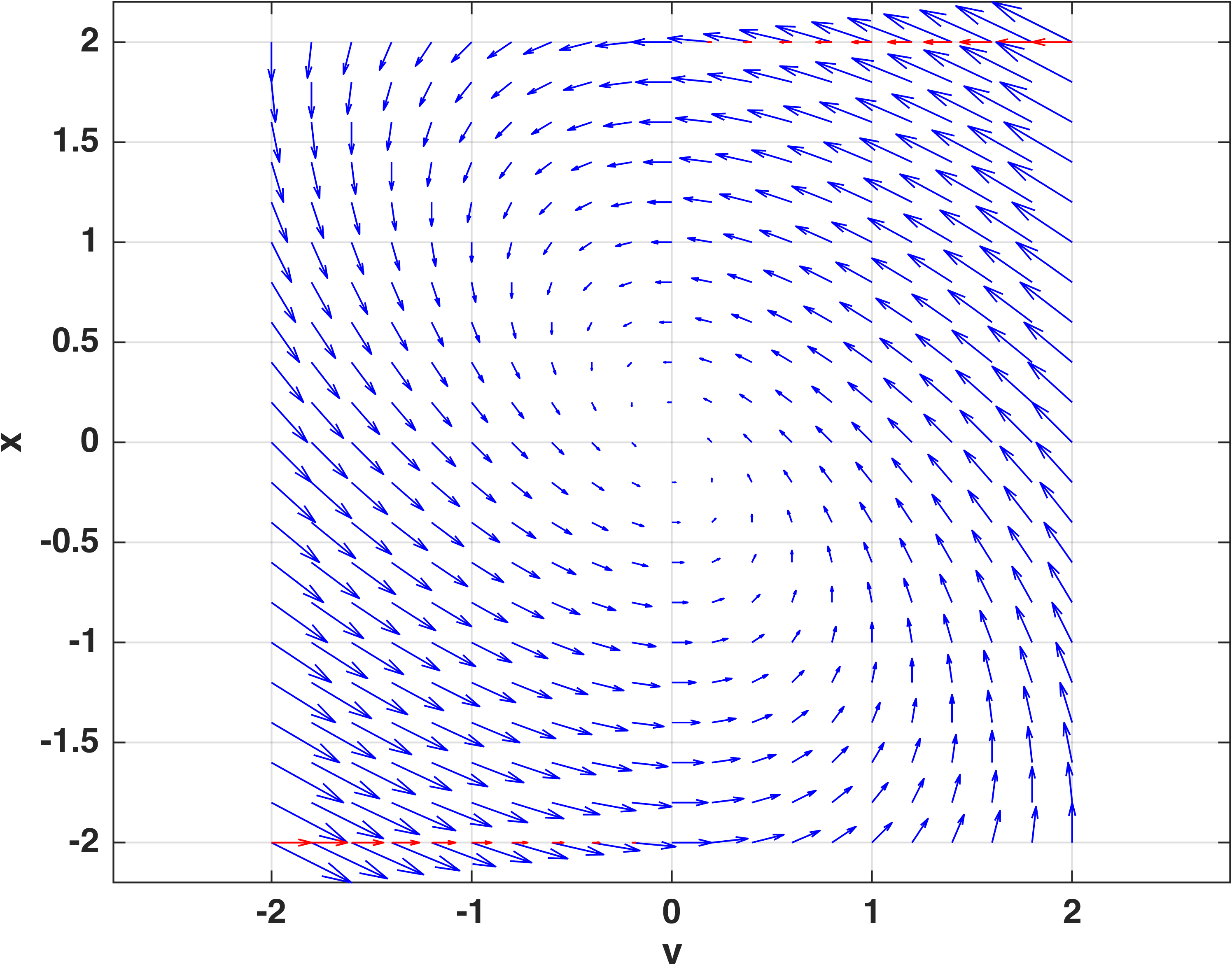
  Figure 3: Constrained second-order dynamics with a plastic velocity increment at the constraint

  We assess now the equivalent position dynamics with a Dirac constraint force by multiplying from the left with ${\bf M}^{-1}$ and using Theorem 2

  $$\left(\begin{array}[]{c}\dot{v}\\ \dot{x}\end{array}\right) = \left(\begin{array}[]{cc}-1&-1\\ 1&0\end{array}\right)\left(\begin{array}[]{c}v\\ x\end{array}\right)-\left(\begin{array}[]{c}u(t)\\ 0\end{array}\right)+\frac{1}{3}\left(\begin{array}[]{cc}2&-1\\ -1&2\end{array}\right)\left(\begin{array}[]{c}0\\ 1\end{array}\right)\lambda_{j}\theta(g_{j})$$ (62)

  $$= \left(\begin{array}[]{cc}-1&-1\\ 1&0\end{array}\right)\left(\begin{array}[]{c}v\\ x\end{array}\right)-\left(\begin{array}[]{c}u(t)\\ 0\end{array}\right)+\left(\begin{array}[]{c}-\frac{1}{3}\theta(g_{j})+\frac{2}{3}\delta(g_{j})\dot{g}_{j}\\ 0\end{array}\right)\lambda_{j}$$ (71)

  with the plastic Dirac impulse force $\lambda_{j}\delta(g_{j})\dot{g}_{j}$ whose transfered impulse over the collistion time instance is $\lambda_{j}\delta(g_{j})\dot{g}_{j}dt=\lambda_{j}$. The collision dynamics (71) with a plastic collision velocity increment $\lambda_{j}=-\frac{3}{2}v$ is shown in figure 3. The equivalent plastic force dynamics is shown in figure 4.

  The fully elastic collision with $\lambda_{j}=-3v$ is shown in figure 5. At the activation of the constraint term the velocity jumps from $\pm v$ to $\mp v$ not changing the contraction field around $v,x$ in the equivalent position dynamics of figure 5.

  

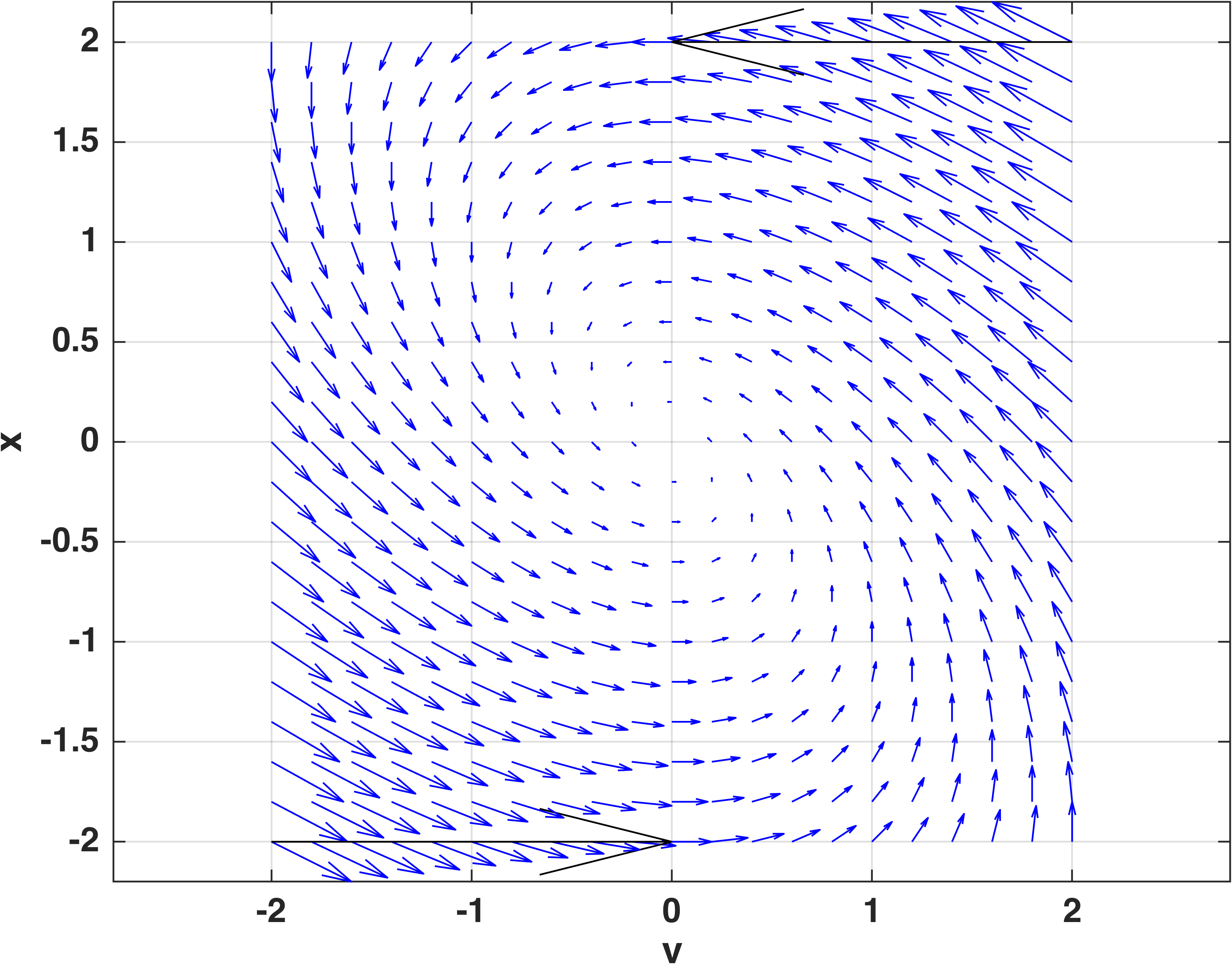
  Figure 4: Constrained second-order dynamics with a plastic Dirac force at the constraint

  

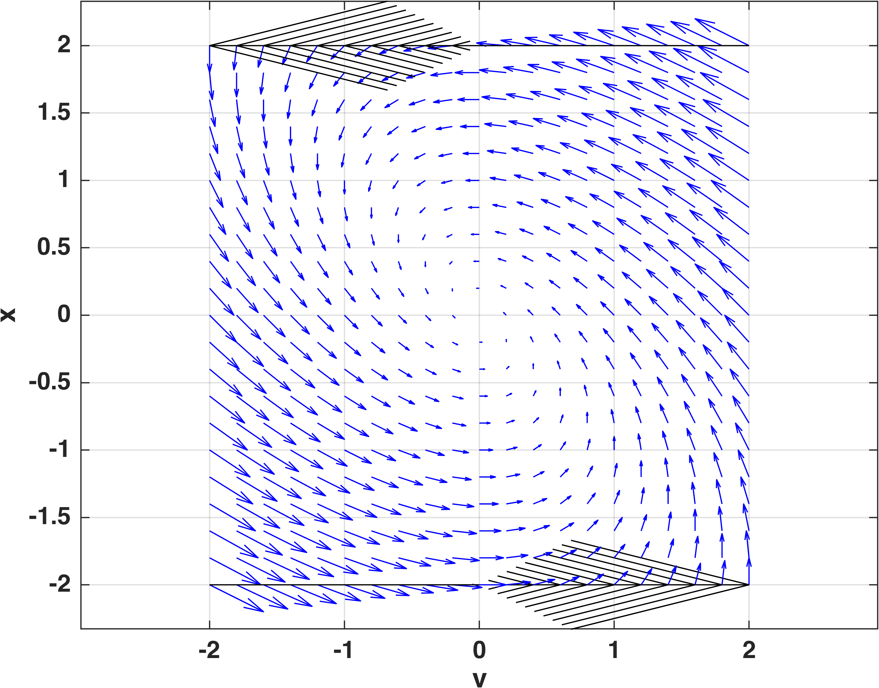
  Figure 5: Constrained second-order dynamics with a fully elastic Dirac force at the constraint

  Note that many practical systems have similar linear constraints, such as end positions or actuator limits. $\Box$

In a constrained Riemann space, as in Theorem 13, the path of minimum length between two points can be shaped by the constraint. For instance, with an identity metric, it needs not be a straight line segment. For a Lagrangian

$$L=\frac{1}{2}\dot{\bf x}^{T}{\bf M}({\bf x})\dot{\bf x}$$

the motion [9, 13] between two connecting points ${\bf x}_{1}(t_{1})$ and ${\bf x}_{2}(t_{2})$ is always a minimization of

$$\int_{{\bf x}_{1}(t_{1})}^{{\bf x}_{2}(t_{2})}Ldt$$

or equivalently

$$\int_{{\bf x}_{1}(t_{1})}^{{\bf x}_{2}(t_{2})}\sqrt{L}dt=\int_{{\bf x}_{1}(t_{1})}^{{\bf x}_{2}(t_{2})}\sqrt{\delta{\bf x}^{T}{\bf M}({\bf x})\delta{\bf x}}$$

so that for a pure kinetic energy the classical Lagrangian dynamics always corresponds to the shortest connection between two points. As we now illustrate, this leads to a new classical interpretation of the duality of particles and waves, by considering the multiple shortest connections between two points in a constrained Riemann space.

• Example 2.4

  : Let us now consider the double slit experiment in Figure 6. We define the geodesic distance on $\mathbb{G}^{2}=\mathbb{R}^{2}\setminus\mathbb{E}^{2}$ rather than on $\mathbb{R}^{2}$, thus excluding the red double slit wall obstacle $\mathbb{E}^{2}$ in Figure 6. The shortest connecting path $s=\min\int_{{\bf x}(s)={\bf x}_{1}}^{{\bf x}_{2}}\sqrt{\delta{\bf x}^{\ast T}\delta{\bf x}}$ (dashed line) from ${\bf x}_{1}$ to ${\bf x}_{2}$ has corner, marked as star in Figure 6, in the two slits.

  A Hamiltonian point mass with energy $h=\frac{1}{2}{\bf p}^{T}{\bf H}({\bf q}){\bf p}$ will get according to Theorem 2 a constraint Dirac collision force $\lambda_{j}\delta(g_{j})\dot{g}_{j}\frac{\partial g_{j}}{\partial{\bf q}}$ at the star corner within the Hamiltonian collision dynamics

  $$\dot{\bf p} = -\frac{\partial h}{\partial{\bf q}}+\sum_{j=1}^{J}\lambda_{j}\delta(g_{j})\dot{g}_{j}\frac{\partial g_{j}}{\partial{\bf q}}$$

  $$\dot{\bf q} = \frac{\partial h}{\partial{\bf p}}$$ (72)

  • This Dirac constraint force can bend the trajectory around the corner which is called difraction. Since the corner has normals in all directions it implies that the trajectory can bend in any direction behind the wall as long as the constraint is not violated.

  • Multiple solutions of the deterministic Hamiltonian dynamics (72) exist here because the Dirac collision force is not Lipschitz continuous. These multiple solutions of a deterministic Hamiltonian (72) are intepreted in quantum physics to be a stochastic distribution of waves.

  • There are two paths of shortest distance in Figure 6, going through slit 1 and slit 2. Both paths have a different distance and travel time. Hence both paths have a different phase angle which allows to compute the quantum state superposition of two particles with a phase shift according to Feynmans path integral formulation [4]. Note the Fenymans path integral is just used here to compute the stochastic distribution of the multiple solutions of a deterministic Hamiltonian (72).

  From this point of view, the only difference of quantum physics to a classical Hamiltonian dynamics is the fact that classical Hamiltonians are defined in unconstrained Riemann spaces whereas quantum physics is defined in constrained Riemann spaces (72). These constraints then imply multiple solutions, due to the non-Lipschitz Dirac collision force (72), which is interpreted as non-determinism in quantum physics.

  

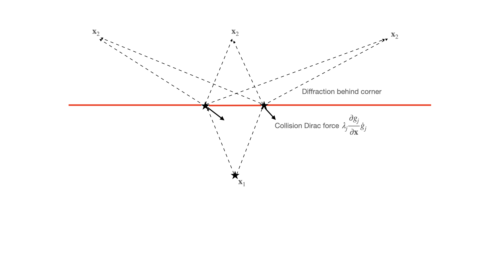
  Figure 6: Constraint Hamiltonian interpretation of double slit experiment

  $\Box$

• Example 2.5

  : Let us now consider the single slit experiment in Figure 7. We define the geodesic distance on $\mathbb{G}^{2}=\mathbb{R}^{2}\setminus\mathbb{E}^{2}$ rather than on $\mathbb{R}^{2}$, thus excluding the red double slit wall obstacle $\mathbb{E}^{2}$ in Figure 6. The shortest connecting path $s=\min\int_{{\bf x}(s)={\bf x}_{1}}^{{\bf x}_{2}}\sqrt{\delta{\bf x}^{\ast T}\delta{\bf x}}$ (dashed line) from ${\bf x}_{1}$ to ${\bf x}_{2}$ has two corners, marked as star in Figure 6, in the slit.

  A Hamiltonian point mass with energy $h=\frac{1}{2}{\bf p}^{T}{\bf H}({\bf q}){\bf p}$ will get according to Theorem 2 a constraint Dirac collision force $\lambda_{j}\delta(g_{j})\dot{g}_{j}\frac{\partial g_{j}}{\partial{\bf q}}$ at the star corner within the Hamiltonian collision dynamics

  $$\dot{\bf p} = -\frac{\partial h}{\partial{\bf q}}+\sum_{j=1}^{J}\lambda_{j}\delta(g_{j})\dot{g}_{j}\frac{\partial g_{j}}{\partial{\bf q}}$$

  $$\dot{\bf q} = \frac{\partial h}{\partial{\bf p}}$$ (73)

  • This Dirac constraint force can bend the trajectory within the slit, which is called difraction. Since the corner has normals in all directions it implies that the trajectory can bend in any direction behind the wall as long as the constraint is not violated. The collision force applies to particles on the left, right and middle of the slit due to the size of the particle.

  • Multiple solutions of the deterministic Hamiltonian dynamics (73) exist here since the Dirac collision force is not Lipschitz continuous. These multiple solutions of a deterministic Hamiltonian (73) are interpreted in quantum physics to be a stochastic distribution of waves.

  • There are several paths of shortest distance in Figure 6, going through the slit of finite size. All paths have a different distance and travel time. Hence all paths have a different phase angle which allows to compute the quantum state superposition of two particles with a phase shift according to the Feynman path integral formulation [4]. Note the Fenyman path integral is just used here to compute the stochastic distribution of the multiple solutions of a deterministic Hamiltonian (73).

  From this point of view, the only difference of quantum physics to a classical Hamiltonian dynamics is the fact that classical Hamiltonians are defined in unconstrained Riemann spaces whereas quantum physics is defined in constrained Riemann spaces (73). These constraints then imply multiple solutions, due to the non-Lipschitz Dirac collision force (73), which is interpreted as non-determinism in quantum physics.

  

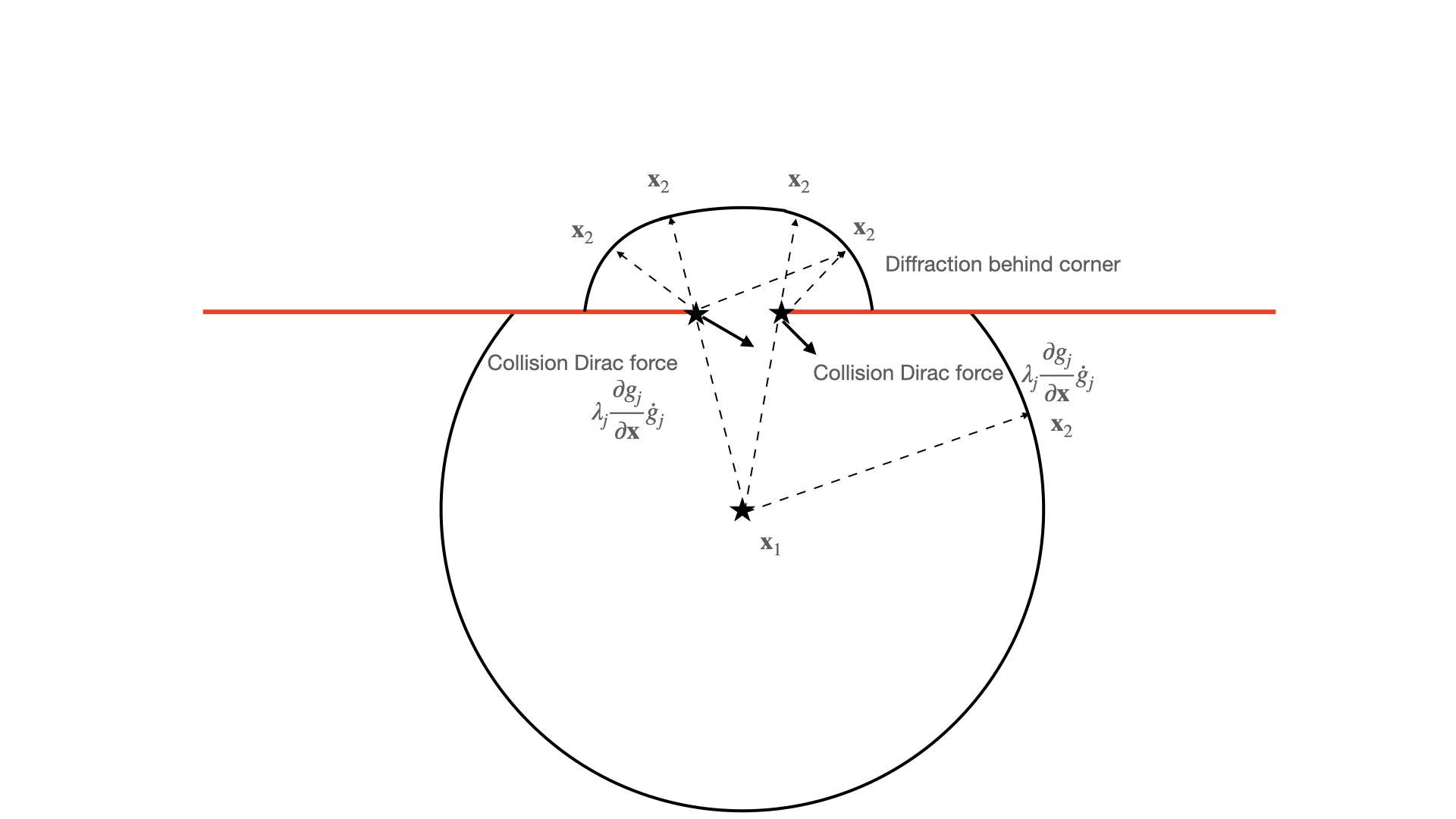
  Figure 7: Constraint Hamiltonian interpretation of single slit experiment

  $\Box$

3 Summary

This paper extends continuous contraction theory of non-linear dynamics to non-linear inequality constraints:

• The contraction behaviour of the constrained dynamics is the covariant derivative of the system dynamics, from the original contraction theorem [5], plus the second covariant derivative of the inequality constraint on the constraint as defined in Theorem 13.

• For Hamiltonian dynamics a Dirac collision force in Theorem 2 has an equivalent position dynamics to the velocity constraint dynamics of heorem 13.

Practical applications include controllers constrained to an operational envelope, trajectory control considering moving obstacles as constraints, and a classical Hamiltonian interpretation of the single and two slit experiments of quantum mechanics, among others.

Example 6 and Example 7 showed that in this context the only difference between quantum physics and classical Hamiltonian physics is the fact that classical Hamiltonians are defined in unconstrained Riemann spaces leading to a single deterministic solution of the Lipschitz Hamiltonian dynamics. The non-Lipschitz Dirac collision force, which is introduced by constraints in quantum physics, leads to a set of multiple solutions of a deterministic Hamiltonian 72, which is intepreted as non-determinism in quantum physics.

The results of this paper are extended to the discrete-time case in [8]. This allows contraction of discrete-time learning in piece-wise linear neuronal networks to be assessed.

Acknowledgements   We thank Paul Schiefer and Lukas Huber for the simulations of this paper. We also thank Philipp Gassert for fruitful discussions in the context of this paper.

References

- [1] Bronstein, Semendjajew, Taschenbuch der Mathematik, Teubner, 1991.
- [2] Bryson A., Yu-Chi H., Applied Optimal Control, Taylor and Francis, 1975.
- [3] https://en.wikipedia.org/wiki/Double-slit_experiment
- [4] Feynman’s path integral formulation https://en.wikipedia.org/wiki/Path_integral_formulation
- [5] Lohmiller, W., and Slotine, J.J.E., On Contraction Analysis for Nonlinear Systems, Automatica, 34(6), 1998.
- [6] Lohmiller, W., and Slotine, J.J.E., Nonlinear Process Control Using Contraction Theory, A.I.Ch.E. Journal, March 2000.
- [7] Lohmiller, W., and Slotine, J.J.E., Contraction Theory with Inequality Constraints, arXiv:1804.10085, 2023.
- [8] Lohmiller, W., Gassert P. and Slotine, J.J.E., MinMax Networks, arXiv, 2023
- [9] Lovelock D., and Rund, H., Tensors, Differential Forms, and Variational Principles, Dover, 1989.
- [10] Moore-Penrose Inverse https://en.wikipedia.org/wiki/Moore–Penrose_inverse
- [11] Nguyen, H.D., Vu, T.L., Slotine, J.J.E., and Turitsyn, K., ”Contraction Analysis of Nonlinear DAE Systems,” I.E.E.E. Transactions on Automatic Control, 2020
- [12] Tabareau, N., Bennequin, D., Berthoz A., Slotine J.J.E., and Girard, B., ”Geometry of the Superior Colliculus Mapping and Efficient Oculomotor Computation,” Biological Cybernetics, 97(4), 2007
- [13] Tolman R.C., Relativity Thermodynamics and Cosmology, Dover Publications, 1934.