Bayesian atomic clock locking

State-of-the-art atomic clocks occupy a crucial position in both fundamental science and practical technology. Generally, their stability is limited by the standard quantum limit, which scales as $1/\sqrt{N}$ in terms of the particle number $N$ or $1/\sqrt{T}$ in terms of the interrogation time $T$. On one hand, it is well-known that the scaling in terms of $N$ can be improved by employing quantum entanglement. On the other hand, the scaling in terms of $T$ can be improved by using well-designed Bayesian estimation. Here, by designing an adaptive Bayesian frequency estimation algorithm for a cold-atom coherent-population-trapping clock, we demonstrate the Heisenberg-limited sensitivity and achieve high-precision locking of the clock transition frequency. Benefit from the Heisenberg-limited sensitivity, the fractional frequency stability is improved to $4.2\times 10^{-12}/\sqrt{\tau}$, which is 6 times better than that of the conventional locking. Our work not only gives an alternative way to lock atomic clocks, but also provides promising applications in other quantum sensors, such as, quantum magnetometers and atomic interferometers.

Introduction

Atomic clocks work on precise detection of the transition frequency between two specific atomic levels and simultaneous synchronization between the clock transition and a local oscillator (LO)  (?, ?). State-of-the-art atomic clocks not only can be employed for practical applications, such as time-keeping, global satellite positioning systems and telecommunications, but also can be used to search new physics  (?, ?, ?, ?, ?, ?). Usually, the measurement noise is fundamentally dominated by quantum projection noise (QPN). Based upon the Ramsey interferometry, the QPN-limited fractional stability can be given by $\sigma(N,T,\tau)\propto\sqrt{\frac{\zeta^{2}}{N}}\sqrt{\frac{\kappa^{2}}{T}}\sqrt{\frac{1}{\tau}}$, where $\tau$ is the averaging time. $\zeta$ characterizes the QPN reduction among atoms, and $\zeta=1$ for $N$ uncorrelated atoms. $\kappa$ characterizes noise reduction with the interrogation time $T$, and $\kappa=1$ for independent measurements. Reducing the impact of QPN will improve the stability limits, which not only retrenches the averaging time, but also promises to open new opportunities in exploring new physics. For a given $\tau$, reducing $\zeta$ and $\kappa$ can effectively improve the stability.

To reduce $\zeta$, one can use quantum entanglement such as spin squeezing, which has been demonstrated in proof-of-principle experiments  (?, ?, ?, ?, ?, ?, ?, ?, ?, ?, ?). Although spin-squeezing in atomic clocks may enhance their stability, metrological applications require direct observation of stability enhancement without post-processed removal of technical noise  (?, ?). Alternatively, one can reduce $\kappa$ to increase the stability. Using well-designed Bayesian estimation algorithms with different interrogation times, it may be improved to the Heisenberg limit  (?, ?, ?), i.e., $\kappa^{2}\propto 1/T$, which has been applied to measure magnetic fields  (?, ?, ?). However, the Bayesian estimation algorithms have never been utilized to improve atomic clocks.

In this article, we experimentally demonstrate a Bayesian frequency estimation (BFE) algorithm via coherent-population-trapping (CPT) in an ensemble of laser-cooled ${}^{87}{\rm Rb}$ atoms and use it to achieve the high-precision closed-loop locking of a cold-atom CPT clock. The BFE algorithm is designed to measure ${}^{87}{\rm Rb}$ clock transition frequency via exponentially increasing the interrogation time in CPT-Ramsey interferometry and adaptively adjusting the LO frequency during Bayesian updates. The standard deviation of our protocol obeys the Heisenberg scaling $(\propto 1/T)$, which is better than the conventional standard quantum limit (SQL) scaling $(\propto 1/\sqrt{T})$. In further, we lock a cold-atom CPT clock via our BFE and yield a fractional frequency stability of $4.2\times 10^{-12}/\sqrt{\tau}$, which has been improved 6 times from that of the proportional-integral-differential (PID) locking. Applying these results to many-body quantum systems, one will suppress the QPN in the terms of both particle number $N$ and interrogation time $T$ and it gives a great promise for improving sensitivity of practical quantum sensors.

Results

Experimental system

Instead of using a microwave cavity, CPT  (?) interrogates the atomic transitions of alkali atoms optically. Therefore, CPT atomic clocks have an advantage of low power consumption and small size, which is suitable for developing chip-scale atomic clocks  (?, ?, ?). The experimental setup of cold-atom CPT system is similar to our previous work  (?, ?) and is shown in Fig. 1. The details can be seen in the Materials and Methods. We utilize a single-$\Lambda$ CPT scheme (Fig. 1A) to avoid time-dependent intervening between multi-path CPT in the $\textrm{lin}\ \parallel\ \textrm{lin}$ or $\textrm{lin}\perp\ \textrm{lin}$ scheme  (?, ?, ?, ?, ?). In a CPT-Ramsey interferometry, the probability amplitude of the excited state undergoing is given by $P_{\rm{e}}=\alpha e^{-\alpha\Gamma\tau_{d}}[1-(1-e^{-\alpha\Gamma\tau_{p}})|\sec(\alpha)|\times\cos{(f-f_{c}+f_{s})T_{R}}]$, where $\alpha=\Omega^{2}/(\Gamma^{2}+3\Omega^{2}+4\delta^{2})$ represents the interaction with the CPT pulse, $T_{R}$ is the Ramsey time, $\Omega$ is the average Rabi frequency, $\delta$ is the single-photon detuning, $\tau_{p}$ and $\tau_{d}$ are CPT preparation pulse duration and CPT detection pulse duration, $f_{c}$ is the clock transition frequency, $f_{s}$ is the $T_{R}$-dependent frequency shift and $\Gamma$ is the decay rate of the excited state. In our experiment, only the LO frequency $f$ and the Ramsey time $T_{R}$ are tunable, thus the transmission signal becomes proportional to the cosine term, i.e., $S_{TS}\propto\cos{(f-f_{c}+f_{s})T_{R}}$.

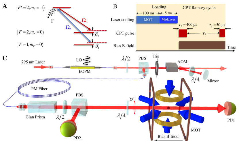
Figure 1: Experimental scheme and setup. (A) A typical three-level $\Lambda$ system in ${}^{87}\rm Rb$. In our experiment, the two clock states $(|F=1,m_{F}=0\rangle\$ and $|F=2,m_{F}=0\rangle)$ are coupled through the excited state $|F^{\prime}=2,m_{F}=-1\rangle$. (B) The timing sequence for an experimental cycle. The loading process contains 100 ms MOT and 5 ms molasses. The CPT-Ramsey process includes a 400 $\rm\mu s$ preparation pulse $\tau_{p}$, a Ramsey time $T_{R}$ and a 50 $\rm\mu s$ detection pulse $\tau_{d}$. The bias magnetic field aligned with the CPT laser beam is applied in the CPT-Ramsey process to split the Zeeman sublevels. (C) Experimental setup. The CPT beam is generated and modified by a fiber-coupled EOPM, an AOM and a Glan prism. To increase signal robustness to power noise, the CPT beam is separated into a transmission beam and a reflected beam by a half-wave plate and a PBS. The $\sigma-\sigma$ configuration of the CPT beam is realized by a quarter-wave plate according to the bias B-field. AOM: acousto-optic modulator, EOPM: electro-optic phase modulator, GP: Glan prism, PBS: polarization beam splitter, PD: photodetector, $\lambda/2$: half-wave plate, $\lambda/4$: quarter-wave plate.

Bayesian frequency estimation

The Bayesian estimation relies on updating the current knowledge of parameters after each experiment by means of Bayes’ law. It is particularly suitable for adaptive experiments in which measurement can be optimized based on the current knowledge of parameters. The adaptivity can improve sensitivity and save time compared with the frequentist estimation. It has been demonstrated that the sensitivity of Ramsey interferometry via single spin systems can surpass the SQL  (?, ?, ?, ?, ?). However single spin systems can only provide a binary data in each measurement and the efficiency is easily affected by quantum shot noise and decoherence. Quantum sensors with atomic ensembles have the advantages of larger particle number $N$ and higher signal-to-noise ratio. Below we present how Bayesian estimation can be used to improve the stability of atomic clocks based upon ensembles.

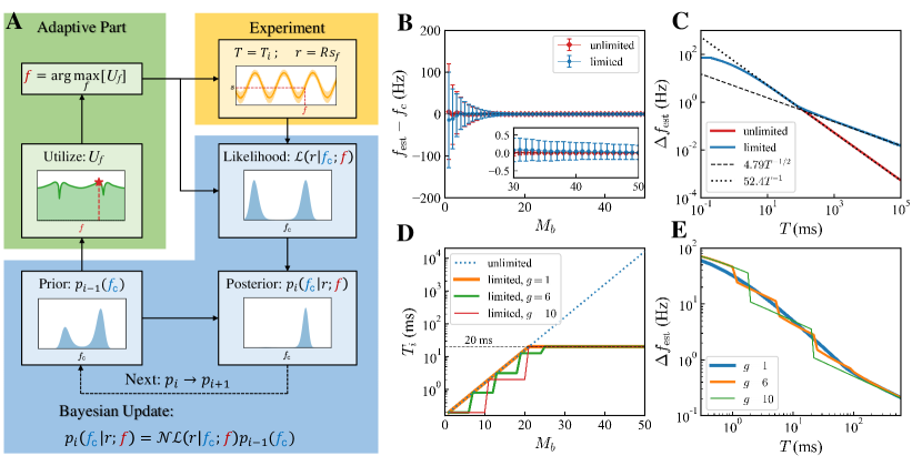
Figure 2: Schematic of Bayesian frequency estimation (BFE) algorithm and numerical results. (A) Schematic of BFE algorithm used in our experiment. Given a prior function $p_{i-1}$ obtained in the previous update, a likelihood function is accordingly obtained and the posterior function is updated through the Bayes’ formula Eq. 3. The likelihood function is obtained with the LO frequency $f$ optimized by the Utilize function Eq. 5. (B) Numerical results with freely increasing the individual interrogation time $T_{i}$ and with limitation that $T_{i}\leq T_{max}$ are represented by red and blue lines respectively. The errorbars are the standard deviations. (C) The standard deviations of B while the measurement times is up to $50$. The black dotted and dashed lines are asymptotes for the two cases respectively. (D) The individual interrogation time $T_{i}$ versus the measurement times $M_{b}$ with $g=1,6,10$. (E) The standard deviation versus the total interrogation time $T$ for $g=1,6,10$. They all converge to the same level after $50$ measurements.

In the Bayesian frequency estimation based upon Ramsey interferometry, the normalization of Ramsey signal $S_{TS}$ can be expressed as

$$s_{f}=\frac{1}{2}[1-\cos{2\pi(f-f_{c}+f_{s})T_{R}}]$$ (1)

The normalization is feasible as long as more than a period of oscillation can be achieved. In the Ramsey interferometry via single-particle systems, the likelihood function reads $\mathcal{L}_{u}(u|f_{c},f)=\frac{1}{2}[1+(-1)^{u}\cos{2\pi(f-f_{c}+f_{s})T_{R}}]$, where $u=0$ or $1$ stand for the particle occupying the clock state $|F=1,m_{F}=0\rangle$ or $|F=2,m_{F}=0\rangle$ respectively. In the CPT-Ramsey interferometry, the signal of each measurement is provided by an ensemble of atoms rather than a single atom. Thus, the likelihood function can be approximated by a Gaussian distribution function  (?),

$$\mathcal{L}(r|f_{c},f)=\frac{1}{\sqrt{2\pi}\sigma}\exp{\left[-\frac{(r-R\mathcal{L}_{u}(1|f_{c},f))^{2}}{2\sigma^{2}}\right]}$$ (2)

where $\sigma^{2}=R\mathcal{L}_{u}(0|f_{c},f)\mathcal{L}_{u}(1|f_{c},f)\approx r(R-r)/R$, the total effective atom number $R$ with $r$ atoms occupying the excited state of the clock transition $\left|F=1,m_{F}=0\right\rangle\leftrightarrow\left|F=2,m_{F}=0\right\rangle$. Here, $R$ is set according to the signal-to-noise ratio in experiments. In our experiments, it is appropriate to set $R=50$. From an initial prior function $p_{0}(f_{c})$ as a Gaussian function with standard deviation $\sigma=0.9$  (?), a corresponding posterior function in the $i$-th Bayesian update is calculated through Bayes’ formula,

$$p_{i}(f_{c}|r;f)=\mathcal{N}\mathcal{L}(r|f_{c},f)p_{i-1}(f_{c})$$ (3)

where $\mathcal{N}$ is a normalization factor. An estimator of $f_{c}$ and its standard deviation can be given as $f_{\rm{est}}^{(i)}=\int{p_{i}(f_{c}|r;f)f_{c}\mathrm{d}f_{c}}$ and $\Delta f_{\rm{est}}^{(i)}=\sqrt{\int{p_{i}(f_{c}|r;f)f_{c}^{2}\mathrm{d}f_{c}}-(\int{p_{i}(f_{c}|r;f)f_{c}\mathrm{d}f_{c}})^{2}}$. The next update is done by inheriting the posterior function as the next prior function $p_{i+1}(f_{c})=p_{i}(f_{c}|r;f)$.

For the periodic probability distribution such as Eq. 1 and the Gaussian likelihood such as Eq. 2, it is suggested to use the adaptive strategy with exponentially sparse times  (?, ?, ?, ?, ?, ?). To achieve the frequency estimation, the LO frequency is adaptively changed according to posterior distribution during Bayesian updates. The procedure of BFE algorithm is sketched in Fig. 2A. Initially, the interrogation time $T_{0}$ and the LO frequency $f$ should be pre-set. Here, we denote the interrogation time used in the $i$-th Bayesian update as $T_{R}^{(i)}\equiv T_{i}$. Initial probability distribution that $f_{c}$ belongs to, is set in the frequency range interval of 5 kHz according to the initial interrogation time $T_{0}=0.2$ ms. After the update via Eq. 3, we change $T_{i}$ as an exponential form for the iteration,

$$T_{i}=\begin{cases}T_{0}a^{i},&i/g\in\mathbb{N^{+}}\\ T_{i-1},&i/g\notin\mathbb{N^{+}}\end{cases}$$ (4)

where $\mathbb{N^{+}}$ is the set of positive integers, $a$ is a parameter that determines the increasing speed of $T_{i}$ and $g$ is a positive integer that determines when $T_{i}$ increases. As $T_{i}$ increases, the corresponding frequency range interval is turned into $[f_{\rm{est}}^{(i)}-1/2T_{i},f_{\rm{est}}^{(i)}+1/2T_{i}]$. The interrogation time $T_{i}$ in our experiment is limited up to $T_{max}=20\rm$ ms because the atoms are freely falling out of the CPT beam if $T_{i}>T_{max}$.

To determine the LO frequency $f_{i}$ for the $i$-th update, we use the expected gain in Shannon information of the posterior function  (?). Different from Ref.  (?) where summation over many single-shot measurement is used, we measure an ensemble of $R$ atoms and the Utilize function becomes,

$$U_{f}=\sum_{r=0}^{R}{U_{r,f}\int{\mathcal{L}(r|f_{c},f)p(f_{c}){\rm d}f_{c}}}$$ (5)

where

$$U_{r,f}=\int{p(f_{c}|r;f)\ln{[p(f_{c}|r;f)]}{\rm d}f_{c}}-\int{p(f_{c})\ln{[p(f_{c})]}{\rm d}f_{c}}$$ (6)

is the expected gain in Shannon information of the posterior function with respect to the prior function. The LO frequency $f_{i}$ is chosen as the one that maximizing $U_{f_{i}}$. Once $f_{i}$ and $T_{i}$ are given, a measurement can be made to obtain a normalized signal $s_{f_{i}}$. Due to the $T_{i}$-dependent frequency shift $f_{s}$ in the CPT-Ramsey interferometry, a measurement of $f_{s}$ prior to the update should be made for a compensation (see Supplementary Materials). Instead of updating every step with $g=1$ (see Fig. 2D), we find that this complexity can be reduced by changing $T_{i}$ every $g$ times, e.g. $g=6$ and $g=10$ in our experiments. This increasing rule for $T_{i}$ is different from the one used in Ref.  (?), but $\Delta f_{\rm est}$ can still achieve the Heisenberg-limited scaling and even have better dynamic range.

The performances of BFE algorithm is shown in Fig. 2 through numerical simulations. By setting $a=1.26$, the estimated value $f_{\rm est}$ is gradually converged to the clock transition frequency $f_{c}$ after several iterations. The scaling of the standard deviation $\Delta f_{\rm est}$ versus the total interrogation time $T=\sum_{i=0}^{M_{b}}{T_{i}}$  (?) obeys the Heisenberg scaling $\propto 1/T$ until $T_{i}$ reaches the maximum limited time $T_{max}$. If the interrogation time $T_{i}$ can increase unlimitedly, the Heisenberg scaling can always attain. However, there always exists a limited evolution time $T_{max}$ due to decoherence. For a time larger than $T_{max}$, the sensitivity scaling would become the SQL $\propto 1/\sqrt{T}$ (Fig. 2C). Fortunately, since the scaling is inversely proportional to the total interrogation time $T=\sum_{i=0}^{M_{b}}{T_{i}}$ rather than a single Ramsey interrogation time $T_{i}$, the scaling $\propto 1/T$ can be preserved for $T>T_{max}$ in which the sensitivity scaling for conventional Ramsey scheme already becomes the SQL ($\propto 1/\sqrt{T}$) (see Supplementary Materials). Simulations with $g=1$, $g=6$ and $g=10$ suggest that the standard deviations with different $g$ converge to the same value (Fig. 2D and Fig. 2E). Therefore, we can remarkably reduce the measurement times for $f_{s}$ through changing $T_{i}$ every $g$ times. Moreover, the case of $g>1$ can even has better dynamic range (see Supplementary Materials). Numerically, we find that the value of $a$ has no effect on the convergence as long as the total integration time $T$ is long enough, but has a slight influence on the dynamic range (see Supplementary Materials).

We use the BFE algorithm to measure the clock transition frequency of ${}^{87}{\rm Rb}$ atoms via CPT in a cold atomic ensemble. The experiment is performed automatically with the help of a computer including the BFE algorithm and digital I/O devices. The BFE algorithm used in our experiment is executed individually to the numerical simulation, except the parameter $r$ that is dependent on the normalized Ramsey signals $s_{f}$. By choosing $T_{0}=0.2$ ms, without loss of generality, we set the frequency range $[f_{c}-3~{}{\rm kHz},f_{c}+2~{}{\rm kHz}]$ as the initial interval. As $T_{0}$ and $a$ are pre-set, we can compensate the $T_{i}$-dependent frequency shift $f_{s}$ via adding it to the LO frequency as $f^{\prime}_{i}=f_{i}+f_{s}$. Then the BFE algorithm provides two varying parameters $T_{i}$ and $f^{\prime}_{i}$ in each update according to Eqs. 4 and 5. The two parameters are sent to the digital I/O devices that control a FPGA to generate a CPT-Ramsey sequence and scan the LO frequency to acquire the CPT-Ramsey fringe. The normalized signal $s_{f_{i}}$ is extracted by cosine fitting of the CPT-Ramsey fringe. The LO is referenced to a high-performance rubidium atomic clock with stability of $6\times 10^{-13}$ at 1 s and $1\times 10^{-12}$ at 100 s.

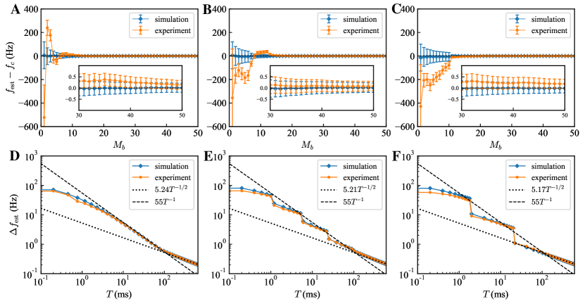
Figure 3: The converge of the estimated frequency and the Heisenberg-limited sensitivity scaling. The results from the experiment where $T_{i}$ increases in every Bayesian update ($g=1$) is shown in A and D, while the results with $T_{i}$ increasing every $g=6$ and $g=10$ Bayesian updates are shown in B and E, and C and F respectively. The estimated frequency difference versus the measurement times $M_{b}$ are plotted on the top including the corresponding standard deviations shown as errorbars, while the standard deviations versus the total interrogation time $T$ are shown on bottom. We also provide results of numerical simulations for comparison as blue lines and points while the results from experiments are colored by orange. In A, B and C the estimated values and the standard deviation decrease rapidly and we zoom in the last $20$ results in the insets.

Our experimental results are shown in Fig. 3, which include the numerical simulations for comparison. By setting $a=1.26$ and the limited interrogation time $T_{max}=20$ ms, the frequency measurement of $f_{c}$ is implemented for $T_{i}$ increasing every $g=1$, $g=6$ and $g=10$ steps during different Bayesian updates. For $g=10$, only $3$ measurement times for $f_{s}$ is needed, which can save a lot of experimental resources, compared with $21$ times for $g=1$. When the iteration number is small ($M_{b}<10$), the estimated value $f_{est}$ from the experiments deviate from results of simulations under the influence of experimental noises (Fig. 3A, Fig. 3B and Fig. 3C). However, it gradually converges to an acceptable one within $1\sigma$ standard deviation as the Bayesian iteration numbers $M_{b}$ increase. Meanwhile the standard deviations provided by the BFE algorithm agree well with the simulation ones, as shown in Fig. 3D, Fig. 3E and Fig. 3F, which follow the Heisenberg-limited scaling.

Closed-loop locking of the cold-atom CPT clock

Based on the BFE algorithm, we stabilize the LO frequency to the atomic reference and realize the Bayesian closed-loop locking of a cold-atom CPT clock. In the conventional closed-loop locking of an atomic clock, the clock transition frequency is acquired by the alternate measurements of the transition probability at bilateral half-maximum points of atomic resonance line. The corresponding error signal is derived from the transition probability difference and fed back to stabilize the LO frequency by a PID controller, as shown in Fig. 4A. We use a CPT-Ramsey fringe with the Ramsey time $T_{R}=20$ ms to closed-loop lock the cold-atom CPT clock. The error signal $\Delta\nu$ is calculated from $f_{c}^{j}=\frac{S_{TS}(f^{j-1}_{c}+1/2T_{R})-S_{TS}(f^{j-1}_{c}-1/2T_{R})}{4T_{R}P}$, where $f_{c}^{j}$ is the clock transition frequency after the $j$-th feedback cycle and $P$ is the amplitude of $S_{TS}$. The frequency fluctuation $\delta\nu_{j}=f_{c}^{j}-f_{c}$ and the corresponding Allan deviation are shown in Fig. 4B and Fig. 4D (in red colour).

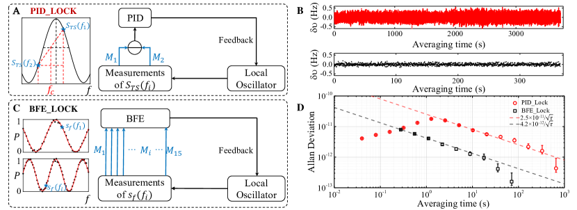
Figure 4: Closed-loop locking of a cold-atom CPT clock. (A) Conventional closed-loop locking of a cold-atom CPT clock via PID controller. The two blue arrows represent two measurements of $S_{TS}$ that is shown by the two blue stars. An error signal is derived by the difference between the two measurements and is sent to the PID controller to realize a feedback on the LO. (B) The frequency fluctuation for conventional closed-loop locking (in red colour) and BFE locking (in black colour). (C) BFE locking of a cold-atom CPT clock. The blue arrows represent 15 measurements of $s_{f}$ for a Bayesian frequency measurement, the normalized signal $s_{f}(f_{i})$ for specific evolution time $T_{i}$ and LO frequency $f_{i}$ are shown by the blue stars left. The estimated transition frequency $f_{c}$ is fed back to the LO. (D) Allan deviation of PID locking and BFE locking. The red dot and dashed line are the results from PID locking, while the black square and dashed line are the results from BFE locking. The stability based on BFE method is typically $4.2\times 10^{-12}/\sqrt{\tau}$, which is 6 times better than that of PID locking, whose frequency stability is $2.5\times 10^{-11}/\sqrt{\tau}$.

In our protocol, the BFE method is carried out to acquire the clock transition frequency and directly fed back to the LO frequency via the error signal $\Delta\nu_{j}=f_{est}^{j}-f_{est}^{j-1}$, where $f_{est}^{j}$ is the $j$-th estimated value of clock transition frequency by $M_{b}$ Bayesian updates (Fig. 4C). This means that we need $M_{b}$ measurements of $s_{f_{i}}$ to achieve one feedback rather than two measurements of $S_{TS}$ for conventional locking. We set $M_{b}=15$ for the closed-loop locking of the cold-atom CPT clock as $f_{est}$ is converged well after 10 updates (see Fig. 3). By increasing $T_{i}$ in every Bayesian update from initial interrogation time $T_{0}=10$ ms to the maximum interrogation time $T_{max}=20$ ms, we realize a tight locking of the cold-atom CPT clock. The results are shown in Fig. 4B and Fig. 4D (in black colour). The frequency fluctuation $\delta\nu_{j}=f_{est}^{j}-f_{c}$ of BFE locking is about 3 times smaller than that of conventional locking with a PID controller.

Finally, we use the Allan deviation to characterize the clock stability. As the transmission signal $S_{TS}$ detected in our experiment is proportional to the excited-state population rather than the clock-state population, the normalized signal $s_{f}$ is used for BFE. $s_{f}$ is obtained by scanning the CPT-Ramsey fringe in our experiment, which is unlike the transition probability at LO frequency $f_{i}$ that could be directly probed by the electron shelving technique in ion trap clocks, fountain clocks and optical lattice clocks  (?, ?, ?). Therefore, we expend more time to measure $s_{f_{i}}$ than $S_{TS}$. Anyway, the clock cycle time (a feedback time) $T_{c}$ contains the total interrogation time $T$ and dead time $T_{d}$. Then the averaging time can be expressed as $\tau=M_{c}T_{c}=M_{c}(T+T_{d})$, where $M_{c}$ is the total feedback number. Here, we use a total interrogation time of a feedback cycle $T=278.5$ ms for BFE locking while $T=40$ ms is used for the conventional locking. Due to the indirect detection of $s_{f}(f_{i})$, the dead time is different for the two locking methods. To facilitate the comparison of the two methods without loss of generality, the dead time is ignoring when we calculate the Allan deviation. We achieve a stability of $4.2\times 10^{-12}/\sqrt{\tau}$ for the BFE locking, which is 6 times better than that of $2.5\times 10^{-11}/\sqrt{\tau}$ for the PID locking. By setting $\tau$ as unit time, the fractional stability $\sigma(N,T,\tau)\propto\Delta f_{est}$. Owing to the $1/T$-scaling frequency measurement assisted by BFE, our cold-atom CPT clocks with BFE locking has an enhancement of stability (see Supplementary Materials). Our BFE locking method could be directly extended to the ion trap clocks, fountain clocks and optical lattice clocks, which would be easier to implement than the cold-atom CPT clock as the transition probability can be directly measured via probing the clock-state population.

Discussion

In conclusion, we experimentally demonstrate a cold-atom CPT clock locking with BFE algorithm, which exhibits better stability than conventional ones. The BFE algorithm is carried out to measure ${}^{87}{\rm Rb}$ clock transition frequency via exponentially step-wise increasing the interrogation time of CPT-Ramsey interferometry and adaptively adjusting the LO frequency during Bayesian updates. The sensitivity versus the interrogation time beats the standard quantum limit and reaches the Heisenberg-limited scaling. Further we lock a cold-atom CPT clock with BFE technique and yield its stability being 6 times better than that of conventional PID locking. Our Bayesian atomic clock locking is also suitable to lock other atomic clocks such as ion trap clocks, fountain clocks and optical lattice clocks, not only benefited from long interrogation time, but also the direct detection of clock-state population.

In our experiment, the precision limit is set by the limited interrogation time $T_{max}$ of our experimental system. Thus, the stability can be improved when long $T_{max}$ is available, such as, the cold atoms in optical lattice may have a $T_{max}$ up to tens of seconds  (?, ?). Besides, to improve the efficiency, one can adopt Markov-chain Monte Carlo (MMC) and particle filter method  (?, ?, ?) to efficaciously reduce the amount of calculation in Bayesian updates. Applying this algorithm to many-body quantum systems  (?, ?, ?, ?), the quantum projection noises can be further suppressed via reducing both $\zeta$ and $\kappa$ simultaneously.

Materials and Methods

Experimental setup

The single-$\Lambda$ CPT connects the clock states $|F=1,m_{F}=0\rangle\ \rm{and}\ |F=2,m_{F}=0\rangle$ through the excited state $|F^{\prime}=2,m_{F}=-1\rangle$. A three-dimensional magnetic-optical trap (MOT) is adopted for 100 ms followed by a 5 ms molasses, which can trap and cool approximately $10^{7}$ ⁸⁷Rb atoms to 20 $\rm\mu K$. At this moment, the atoms are fallen freely and interrogated by left-circularly polarized CPT light in a magnetic field of 35 mG. The CPT beam is generated from a laser modulated by a fiber-coupled electro-optic phase modulator (EOPM) at 6.835 GHz, which is equal to the ⁸⁷Rb ground-state hyperfine splitting frequency. The optical carrier and positive first-order sideband are set as equal intensity and couple the clock states to the excited state. An acousto-optic modulator (AOM) is used to generate the CPT pulses. After a fiber, a Glan prism is used to purify the polarization. We use a timing diagram of a 400 $\rm\mu s$ CPT preparation pulse $\tau_{p}$ followed by an interrogation time $T_{R}$ and a 50 $\rm\mu s$ detection pulse $\tau_{d}$ (Fig. 1B). The CPT beam is equally separated into two beams by a half-wave plate and a polarization beam splitter. One beam, whose polarizations are changed to $\sigma^{-}$ by a quarter-wave plate, transmits through the atoms and is detected by the CPT photodetector as $S_{T}$ (PD1 in Fig. 1C) while the other beam is detected by the photodetector as $S_{N}$ (PD2 in Fig. 1C). The transmission signals (TSs) are given by $S_{TS}=S_{T}/S_{N}$, which can reduce the effect of intensity noise on the CPT-Ramsey signals.

The flowing chart of Bayesian frequency estimation (BFE) algorithm

The BFE algorithm used in our experiment is shown in Algorithm 1.

Input :  modified atom number $R$; minimum interrogation time $T_{0}$; maximum interrogation time $T_{\rm max}$; algorithm parameter $a$ and $g$; initial interval $[f_{l},f_{r}]$;

Output : Estimator and uncertainty: $f_{c}^{\rm est}$ and $\Delta f_{c}^{\rm est}$

Initialize : initial prior function $p_{0}(f_{c})=\frac{1}{\sqrt{2\pi}\sigma}\exp{\frac{(f_{c}-\mu)^{2}}{2\sigma^{2}}}$, where $\mu=(f_{l}+f_{r})/2$ and $\sigma=0.9$

[Main Loop]:

for $i=0$ to $50$ do

       [Updates of parameter];

       interrogation time: $T_{i}=\{\begin{array}[]{ll}T_{0}a^{i},&i/g\in\mathbb{N^{+}}\\ T_{i-1},&i/g\notin\mathbb{N^{+}}\\ \end{array}$;

       if $T_{i}>T_{\rm max}$ then

             $T_{i}=T_{\rm max}$

       end if

      length of interval: $f_{lr}=1/T_{i}$;

       if $i>0$ then

             $f_{l}\leftarrow f_{c}^{\rm est}-f_{lr}/2$;

             $f_{r}\leftarrow f_{c}^{\rm est}+f_{lr}/2$;

             reset the prior function $p_{i}(f_{c})=\frac{1}{\sqrt{2\pi}\sigma}\exp{\frac{(f_{c}-\mu)^{2}}{2\sigma^{2}}}$, where $\mu=(f_{l}+f_{r})/2$ and $\sigma=\Delta f_{c}^{\rm est}$

       end if

      LO frequency: $f=\arg{\max_{f}{U(f)}}$ [Ramdom enhancement];

       if $T_{i}>T_{\rm max}$ then

            $f\leftarrow f+\epsilon$, where $\epsilon\sim\mathcal{N}(0,2\Delta f_{c}^{\rm est})$

       end if

      [Experimental measurement];

       frequency shift compensation: $f\leftarrow f+f_{s}$;

       measurement nomalized signal $s_{f}$ using $T_{i}$ and $f_{i}$;

       $r\leftarrow Rs_{f}$;

       [Bayesian update];

       Likelihood function: $\mathcal{L}(r|f_{c},f)=\frac{1}{\sqrt{2\pi}\sigma}\exp{[-\frac{(r-R\mathcal{L}_{u}(1|f_{c},f))^{2}}{2\sigma^{2}}]}$, where $\sigma^{2}=r(R-r)/R$;

       Bayesian update: $p(f_{c})\leftarrow\mathcal{N}\mathcal{L}(r|f_{c},f)p(f_{c})$;

       Estimator: $f_{c}^{\rm est}=\mathbb{E}_{f_{c}\sim p(f_{c})}(f_{c})=\int{f_{c}p(f_{c})\mathrm{d}f_{c}}$;

       Uncertainty: $\Delta f_{c}^{\rm est}=\sqrt{\mathbb{E}_{f_{c}\sim p(f_{c})}(f_{c}^{2})-(\mathbb{E}_{f_{c}\sim p(f_{c})}(f_{c}))^{2}}$;

      

end for

Algorithm 1 Bayesian frequency estimation algorithm for an atomic ensemble

Supplementary materials

This PDF file includes:
Sections SI to SVII
Figs. S1 to S8

References

- 1. E. Pedrozo-Peñafiel, S. Colombo, C. Shu, A. F. Adiyatullin, Z. Li, E. Mendez, B. Braverman, A. Kawasaki, D. Akamatsu, Y. Xiao, V. Vuletić, Entanglement on an optical atomic-clock transition, Nature 588, 414 (2020).
- 2. A. D. Ludlow, M. M. Boyd, J. Ye, E. Peik, P. O. Schmidt, Optical atomic clocks, Rev. Mod. Phys. 87, 637 (2015).
- 3. C. W. Chou, D. B. Hume, T. Rosenband, D. J. Wineland, Optical clocks and relativity, Science 329, 1630 (2010).
- 4. M. S. Safronova, D. Budker, D. DeMille, D. F. J. Kimball, A. Derevianko, C. W. Clark, Search for new physics with atoms and molecules, Rev. Mod. Phys. 90, 025008 (2018).
- 5. V. Schkolnik, D. Budker, O. Fartmann, V. Flambaum, L. Hollberg, T. Kalaydzhyan, S. Kolkowitz, M. Krutzik, A. Ludlow, N. Newbury, C. Pyrlik, L. Sinclair, Y. Stadnik, I. Tietje, J. Ye, J. Williams, Optical atomic clock aboard an earth-orbiting space station (OACESS): enhancing searches for physics beyond the standard model in space, Quantum Sci. Technol. 8, 014003 (2022).
- 6. C. Sanner, N. Huntemann, R. Lange, C. Tamm, E. Peik, M. S. Safronova, S. G. Porsev, Optical clock comparison for lorentz symmetry testing, Nature 567, 204 (2019).
- 7. C. J. Kennedy, E. Oelker, J. M. Robinson, T. Bothwell, D. Kedar, W. R. Milner, G. E. Marti, A. Derevianko, J. Ye, Precision metrology meets cosmology: Improved constraints on ultralight dark matter from atom-cavity frequency comparisons, Phys. Rev. Lett. 125, 201302 (2020).
- 8. M. Takamoto, I. Ushijima, N. Ohmae, T. Yahagi, K. Kokado, H. Shinkai, H. Katori, Test of general relativity by a pair of transportable optical lattice clocks, Nature Photon. 14, 411–415 (2020).
- 9. B. C. Nichol, R. Srinivas, D. P. Nadlinger, P. Drmota, D. Main, G. Araneda, C. J. Ballance, D. M. Lucas, An elementary quantum network of entangled optical atomic clocks, Nature 609, 689–694 (2022).
- 10. J. Appel, P. J. Windpassinger, D. Oblak, U. B. Hoff, N. Kjærgaard, E. S. Polzik, Mesoscopic atomic entanglement for precision measurements beyond the standard quantum limit, PNAS 106, 10960 (2009).
- 11. I. Kruse, K. Lange, J. Peise, B. Lücke, L. Pezzè, J. Arlt, W. Ertmer, C. Lisdat, L. Santos, A. Smerzi, C. Klempt, Improvement of an atomic clock using squeezed vacuum, Phys. Rev. Lett. 117, 143004 (2016).
- 12. T. Takano, M. Fuyama, R. Namiki, Y. Takahashi, Spin squeezing of a cold atomic ensemble with the nuclear spin of one-half, Phys. Rev. Lett. 102, 033601 (2009).
- 13. J. G. Bohnet, K. C. Cox, M. A. Norcia, J. M. Weiner, Z. Li, Z. Chen, J. K. Thompson, Reduced spin measurement back-action for a phase sensitivity ten times beyond the standard quantum limit, Nature Photon. 8, 731 (2014).
- 14. L. Pezzè, A. Smerzi, M. K. Oberthaler, R. Schmied, P. Treutlein, Quantum metrology with nonclassical states of atomic ensembles, Rev. Mod. Phys. 90, 035005 (2018).
- 15. C. Lee, Adiabatic Mach-Zehnder interferometry on a quantized Bose-Josephson junction, Phys. Rev. Lett. 97, 150402 (2006).
- 16. J. Estève, C. Gross, A. Weller, S. Giovanazzi, M. K. Oberthaler, Squeezing and entanglement in a Bose-Einstein condensate, Nature 455, 1216 (2008).
- 17. G. Tóth, I. Apellaniz, Quantum metrology from a quantum information science perspective, J. Phys. A: Math. Theor. 47, 424006 (2014).
- 18. O. Hosten, N. J. Engelsen, R. Krishnakumar, M. A. Kasevich, Measurement noise 100 times lower than the quantum-projection limit using entangled atoms, Nature 529, 505 (2016).
- 19. N. Wiebe, C. Granade, Efficient Bayesian phase estimation, Phys. Rev. Lett. 117, 010503 (2016).
- 20. B. L. Higgins, D. W. Berry, S. D. Bartlett, H. M. Wiseman, G. J. Pryde, Entanglement-free Heisenberg-limited phase estimation, Nature 450, 393 (2007).
- 21. C. L. Degen, F. Reinhard, P. Cappellaro, Quantum sensing, Rev. Mod. Phys. 89, 035002 (2017).
- 22. R. Santagati, A. A. Gentile, S. Knauer, S. Schmitt, S. Paesani, C. Granade, N. Wiebe, C. Osterkamp, L. P. McGuinness, J. Wang, M. G. Thompson, J. G. Rarity, F. Jelezko, A. Laing, Magnetic-field learning using a single electronic spin in diamond with one-photon readout at room temperature, Phys. Rev. X 9, 021019 (2019).
- 23. R. Puebla, Y. Ban, J. Haase, M. Plenio, M. Paternostro, J. Casanova, Versatile atomic magnetometry assisted by Bayesian inference, Phys. Rev. Applied 16, 024044 (2021).
- 24. N. M. Nusran, M. U. Momeen, M. V. Dutt, High-dynamic-range magnetometry with a single electronic spin in diamond, Nature Nanotech. 7, 109 (2012).
- 25. H. R. Gray, R. M. Whitley, J. Stroud, C. R., Coherent trapping of atomic populations, Opt. Lett. 3, 218 (1978).
- 26. M. A. Hafiz, G. Coget, M. Petersen, C. E. Calosso, S. Guérandel, E. d. Clercq, R. Boudot, Symmetric autobalanced ramsey interrogation for high-performance coherent-population-trapping vapor-cell atomic clock, Appl. Phys. Lett. 112, 244102 (2018).
- 27. X. Liu, E. Ivanov, V. I. Yudin, J. Kitching, E. A. Donley, Low-drift coherent population trapping clock based on laser-cooled atoms and high-coherence excitation fields, Phys. Rev. Applied 8, 054001 (2017).
- 28. P. Yun, F. Tricot, C. E. Calosso, S. Micalizio, B. François, R. Boudot, S. Guérandel, E. de Clercq, High-performance coherent population trapping clock with polarization modulation, Phys. Rev. Applied 7, 014018 (2017).
- 29. R. Fang, C. Han, X. Jiang, Y. Qiu, Y. Guo, M. Zhao, J. Huang, B. Lu, C. Lee, Temporal analog of Fabry-Pérot resonator via coherent population trapping, npj Quantum Information 7, 143 (2021).
- 30. C. Han, J. Huang, X. Jiang, R. Fang, Y. Qiu, B. Lu, C. Lee, Adaptive Bayesian algorithm for achieving a desired magneto-sensitive transition, Opt. Exp. 29, 21031 (2021).
- 31. A. V. Taichenachev, V. I. Yudin, V. L. Velichansky, S. A. Zibrov, On the unique possibility of significantly increasing the contrast of dark resonances on the D1 line of 87Rb, Jetp Lett. 82, 398 (2005).
- 32. C. Xi, Y. Guo-Qing, W. Jin, Z. Ming-Sheng, Coherent population trapping-Ramsey interference in cold atoms, Chin. Phys. Lett. 27, 113201 (2010).
- 33. E. Blanshan, S. M. Rochester, E. A. Donley, J. Kitching, Light shifts in a pulsed cold-atom coherent-population-trapping clock, Phys. Rev. A 91, 041401(R) (2015).
- 34. S. V. Kargapoltsev, J. Kitching, L. Hollberg, A. V. Taichenachev, V. L. Velichansky, V. I. Yudin, High-contrast dark resonance in optical field, Laser Phys. Lett. 1, 495 (2004).
- 35. T. Zanon, S. Guerandel, E. de Clercq, D. Holleville, N. Dimarcq, A. Clairon, High contrast Ramsey fringes with coherent-population-trapping pulses in a double Lambda atomic system, Phys. Rev. Lett. 94, 193002 (2005).
- 36. P. Cappellaro, Spin-bath narrowing with adaptive parameter estimation, Phys. Rev. A 85, 030301(R) (2012).
- 37. C. Bonato, M. Blok, H. Dinani, D. Berry, M. Markham, D. Twitchen, R. Hanson, Optimized quantum sensing with a single electron spin using real-time adaptive measurements, Nature Nanotech. 11, 247 (2016).
- 38. H. T. Dinani, D. W. Berry, R. Gonzalez, J. R. Maze, C. Bonato, Bayesian estimation for quantum sensing in the absence of single-shot detection, Phys. Rev. B 99, 125413 (2019).
- 39. A. Lumino, E. Polino, A. S. Rab, G. Milani, N. Spagnolo, N. Wiebe, F. Sciarrino, Experimental phase estimation enhanced by machine learning, Phys. Rev. Applied 10, 044033 (2018).
- 40. R. S. Said, D. W. Berry, J. Twamley, Nanoscale magnetometry using a single-spin system in diamond, Phys. Rev. B 83, 125410 (2011).
- 41. G. Waldherr, J. Beck, P. Neumann, R. S. Said, M. Nitsche, M. L. Markham, D. J. Twitchen, J. Twamley, F. Jelezko, J. Wrachtrup, High-dynamic-range magnetometry with a single nuclear spin in diamond, Nature Nanotech. 7, 105 (2012).
- 42. C. Ferrie, C. E. Granade, D. G. Cory, How to best sample a periodic probability distribution, or on the accuracy of Hamiltonian finding strategies, Quantum Information Processing 12, 611 (2013).
- 43. T. Ruster, H. Kaufmann, M. A. Luda, V. Kaushal, C. T. Schmiegelow, F. Schmidt-Kaler, U. G. Poschinger, Entanglement-based dc magnetometry with separated ions, Phys. Rev. X 7, 031050 (2017).
- 44. W. Nagourney, J. Sandberg, H. Dehmelt, Shelved optical electron amplifier: Observation of quantum jumps, Phys. Rev. Lett. 56, 2797 (1986).
- 45. R. Wynands, S. Weyers, Atomic fountain clocks, Metrologia 42, S64 (2005).
- 46. V. Xu, M. Jaffe, C. Panda, S. Kristensen, L. Clark, H. Müller, Probing gravity by holding atoms for 20 seconds, Science 366, 745 (2019).
- 47. A. Young, W. Eckner, W. Milner, D. Kedar, M. Norcia, E. Oelker, N. Schine, J. Ye, A. Kaufman, Half-minute-scale atomic coherence and high relative stability in a tweezer clock, Nature 588, 408 (2020).
- 48. C. E. Granade, C. Ferrie, N. Wiebe, D. G. Cory, Robust online Hamiltonian learning, New J. Phys. 14, 103013 (2012).
- 49. J. Wang, S. Paesani, R. Santagati, S. Knauer, A. A. Gentile, N. Wiebe, M. Petruzzella, J. L. O’brien, J. G. Rarity, A. Laing, M. G. Thompson, Experimental quantum Hamiltonian learning, Nature Phys. 13, 551 (2017).
- 50. Y. Qiu, M. Zhuang, J. Huang, C. Lee, Efficient Bayesian phase estimation via entropy-based sampling, Quantum Sci. Technol. 7, 035022 (2022).
- 51. S. Nolan, A. Smerzi, L. Pezzè, A machine learning approach to Bayesian parameter estimation, npj Quantum Information 7, 169 (2021).
- 52. G. Carleo, I. Cirac, K. Cranmer, L. Daudet, M. Schuld, N. Tishby, L. Vogt-Maranto, L. Zdeborová, Machine learning and the physical sciences, Rev. Mod. Phys. 91, 045002 (2019).
- 53. L. Pezzè, A. Smerzi, M. K. Oberthaler, R. Schmied, P. Treutlein, Quantum metrology with nonclassical states of atomic ensembles, Rev. Mod. Phys. 90, 035005 (2018).
- 54. R. Elvin, G. W. Hoth, M. W. Wright, J. P. McGilligan, A. S. Arnold, P. F. Griffin, E. Riis, Raman-Ramsey CPT with a grating magneto-optical trap, 2018 European Frequency and Time Forum (EFTF), pp. 61–64.
- 55. Z.-W. Thomas, d. C. Emeric, A. Ennio, Ultrahigh-resolution spectroscopy with atomic or molecular dark resonances: Exact steady-state line shapes and asymptotic profiles in the adiabatic pulsed regime, Phys. Rev. A 84, 062502 (2011).
- 56. P. R. Hemmer, M. S. Shahriar, V. D. Natoli, S. Ezekiel, Ac stark shifts in a two-zone Raman interaction, J. Opt. Soc. Am. B 6, 1519 (1989).
Acknowledgments
Funding: This work is supported by the National Key Research and Development Program of China (2022YFA1404104), the National Natural Science Foundation of China (12025509, 12104521), and the Key-Area Research and Development Program of GuangDong Province (2019B030330001). Author contributions: C.L., B.L. and J.H. conceived the project. Y.Q., J.H. and C.L. developed the physical protocol and performed the theoretical simulations. C.H., Z.M. and B.L. designed the experiment. C.H., Z.M., J.W., C.Z. and M.L. performed the experiment. All authors discussed the results and contributed to compose and revise the manuscript. C.L. supervised the project. Competing interests: The authors declare no competing interests. Data and materials availability: All data needed to evaluate the conclusions in the paper are present in the paper and/or the Supplementary Materials