Optimizing the Collaboration Structure in Cross-Silo Federated Learning

Abstract

In federated learning (FL), multiple clients collaborate to train machine learning models together while keeping their data decentralized. Through utilizing more training data, FL suffers from the potential negative transfer problem: the global FL model may even perform worse than the models trained with local data only. In this paper, we propose FedCollab, a novel FL framework that alleviates negative transfer by clustering clients into non-overlapping coalitions based on their distribution distances and data quantities. As a result, each client only collaborates with the clients having similar data distributions, and tends to collaborate with more clients when it has less data. We evaluate our framework with a variety of datasets, models, and types of non-IIDness. Our results demonstrate that FedCollab effectively mitigates negative transfer across a wide range of FL algorithms and consistently outperforms other clustered FL algorithms.

1 Introduction

Federated learning (FL) is a distributed learning system where multiple clients collaborate to train a machine learning model under the orchestration of the central server, while keeping their data decentralized (McMahan et al., 2017). We focus on cross-silo FL, where clients are organizations with data that differ in their distributions and quantities (Caldas et al., 2018). For example, the clients can be hospitals with varying patient types and numbers (e.g., children’s hospitals, trauma centers). Although cross-silo FL clients can train local models with their own data locally (local training), they participate in FL for a model trained with more data, which potentially performs better than local models.

Traditionally, global FL (GFL) (McMahan et al., 2017; Wang et al., 2020b; Li et al., 2020a) trains a single global model for all clients that minimizes a weighted average of local losses. It is a natural solution when clients have independent and identically distributed (IID) data. However, when clients have non-IID data, GFL may suffer from the negative transfer problem: the global model performs even worse than the local models (Zhang et al., 2021). The negative transfer problem also plagues many personalized FL (PFL) algorithms (Fallah et al., 2020; Dinh et al., 2020; Li et al., 2021). Although these algorithms allow each client to train a personalized model with parameters different from the global model, the regularization of the global model still prevents personalized models from achieving better performance than local models.

One way to avoid negative transfer is clustered FL (CFL) (Sattler et al., 2021; Long et al., 2022; Ghosh et al., 2019). CFL groups clients with similar data distribution into coalitions, and trains FL models within each coalition. As a result, each client only collaborates with other clients in the same coalition. By changing the collaboration structure, CFL can alleviate negative transfer with almost no additional computation and communication costs.

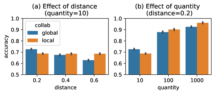
Figure 1: Effects of distribution distance and data quantity. When two clients have large distribution distance or large quantities, the local model performs better than global model.

A natural follow-up question would be what determines the best collaboration structure. We summarize two key factors for characterizing client collaboration: distribution distance and data quantity. We start with a simple 2-client scenario, studying whether the global model or the local model has higher accuracy. As shown in Figure 1, when two clients have small distribution distance and small quantity, the global model has higher accuracy, which is a scenario suitable for GFLs. When the distribution distance between two clients increases (Figure 1(a)), the local model performs better than the global model, showing that distribution distance influences the optimal collaboration structure. Meanwhile, it is often ignored that the data quantity also influences the optimal collaboration structure: given the same distribution distance, when the data quantity increases (Figure 1(b)), the local model also performs better than the global model. In other words, clients with more data are more “picky” in the choice of collaborators.

Previous CFL algorithms (Ghosh et al., 2020; Long et al., 2022; Sattler et al., 2021) generate clusters mainly based on loss values or parameter/gradient similarities, which have the following drawbacks. First, they ignore the influence of quantities, and group clients together, even when these clients have large quantities and prefer local training. Second, most CFL algorithms rely on indirect information of distribution distance, which does not recover the real distribution distance given the high complexity of neural networks (e.g., nonlinearity and permutation invariance). Finally, most CFL algorithms optimize the model parameters and collaboration structure simultaneously. Thus, they reinforce the current collaboration structure and fall into local optima easily, resulting in sub-optimal model performance.

In this paper, we propose FedCollab to optimize for a better collaboration structure. First, we derive a theoretical error bound for each client in the FL system. The error bound consists of three terms: an irreducible minimal error term related to the model and data noise, a generalization error term depending on data quantities, and a dataset shift term depending on pairwise distribution distance between clients. By minimizing the error bounds, FedCollab solves for the optimal collaboration structure with awareness of both quantities and distribution distances. Second, to better estimate pairwise distribution distances without violating the privacy constraint of FL, we use a light-weight client discriminator between each pair of clients to predict which client the labeled data comes from, and train the discriminator within the FL framework. Third, we design an efficient optimization method to minimize the error bound. It requires no model training and solves the collaboration in seconds. Finally, we run FL algorithms within each coalition we identify. Since the model training and collaboration structure optimization are disentangled, FedCollab can be seamlessly integrated with any GFL or PFL algorithms.

Contributions

We summarize our contributions below.

• We derive error bounds for FL clients and summarize two key factors that affect the model performance for each client: data quantity and distribution distance. (Section 3)

• We propose FedCollab to solve for the best collaboration structure, including a distribution difference estimator and an efficient optimizer. (Section 4)

• We empirically test our algorithm with a wide range of datasets, models, and types of non-IIDness. FedCollab enhances a variety of FL algorithms by providing better collaboration structures, and outperforms existing CFL algorithms in accuracy. (Section 5)

2 Related Works

Global Federated Learning

Global federated learning (GFL) aims to train a single global model for private clients, by assuming that all the clients follow the same data distribution. Typically, FedAvg (McMahan et al., 2017) is proposed to minimize a weighted average of local client objectives (e.g., empirical risks). More recently, many efforts (Li et al., 2020a; Karimireddy et al., 2020) have been made to speed up the convergence of FL on top of FedAvg. Another related line of works (Mohri et al., 2019; Li et al., 2020b) is performance fairness aware federated learning, which encourages a uniform distribution of accuracy among clients. However, it is revealed (Zhang et al., 2021) that under severe data heterogeneity among clients, these GFL algorithms suffer from negative transfer with undesirable performance on local clients.

Personalized Federated Learning

In recent years, personalized federated learning has been proposed to deal with statistical data heterogeneity among clients. We roughly group them into two categories: coarse-grained and fine-grained. For coarse-grained PFL (Fallah et al., 2020; Dinh et al., 2020; Li et al., 2021), each client can further optimize a global model (trained with the union of local datasets) with its own data. This kind of PFL algorithm cannot choose which clients to collaborate with, and suffer from negative transfer when the client’s own data distribution is distinct from the population. For fine-grained PFL (Smith et al., 2017), clients can directly collaborate with some of the other clients. However, most of the fine-grained PFL algorithms significantly change the communication protocol of FL or introduce additional communication and computation costs (Smith et al., 2017; Zhang et al., 2021).

Clustered Federated Learning

Similar to our algorithm, clustered federated learning partitions clients into clusters. For example, IFCA (Ghosh et al., 2020) initializes multiple models and lets each client choose one based on the training loss; FeSEM (Long et al., 2022) lets each client choose a cluster with similar weights; and CFL (Sattler et al., 2021) iteratively bipartition the clients based on their cosine similarity of gradients. However, all these methods only consider distribution distances and ignore the importance of data quantities, which also play a key role in collaboration performance. To the best of our knowledge, (Donahue & Kleinberg, 2021) is the only work that considers the quantity in the optimization of the collaboration structure. However, it is limited to linear models with analytical solutions, and only considers a simplified non-IID setting.

3 Analysis of Client Error Bound

In this section, we derive a theoretical error bound to understand how data quantity and distribution distance affect the model performance for each client.

3.1 Setup

We consider a FL system with $N$ clients connected to a central server. Each client $i\in\{1,\cdots,N\}$ has a dataset $\hat{}\mathcal{D}_{i}=\{(\boldsymbol{x}_{k}^{(i)},\boldsymbol{y}_{k}^{(i)})\}_{k=1}^{m_{i}}$ with $m_{i}$ samples drawn from its underlying true data distribution $\mathcal{D}_{i}$, where $\boldsymbol{x}_{k}^{(i)}\in\mathcal{X}$ is the feature and $\boldsymbol{y}_{k}^{(i)}\in\mathcal{Y}$ is the label. We denote $m=\sum_{i=1}^{N}m_{i}$ as the total quantity of samples and $\boldsymbol{\beta}=[\beta_{1},\cdots,\beta_{N}]=[\frac{m_{1}}{m},\cdots,\frac{m_{N}}{m}]$ as the client quantity distribution. Given a machine learning model (hypothesis) $h$ and risk function $\ell$, client $i$’s local expected risk is given by $\epsilon_{i}(h)=\mathbb{E}_{(\boldsymbol{x},\boldsymbol{y})\in\mathcal{D}_{i}}\ell(h(\boldsymbol{x}),\boldsymbol{y})$, and its local empirical risk is given by $\hat{\epsilon}_{i}(h)=\frac{1}{m_{i}}\sum_{k=1}^{m_{i}}\ell(h(\boldsymbol{x}_{k}^{(i)}),\boldsymbol{y}_{k}^{(i)})$. The goal of each client $i\in\{1,\cdots,N\}$ is to find a model $h$ within the hypothesis space $\mathcal{H}$ that minimizes its local expected risk, which we denote as $h_{i}^{*}=\operatorname*{arg\,min}_{h\in\mathcal{H}}\epsilon_{i}(h)$. However, clients can only optimize their models with their finite samples $\hat{}\mathcal{D}_{1},\cdots,\hat{}\mathcal{D}_{N}$. There are several representative options: local training, global FL (GFL), and clustered FL (CFL).

Local Training

In local training, each client trains its own model individually without sharing information with other clients. Each local model minimizes the local empirical risk $\hat{h}_{i}=\operatorname*{arg\,min}_{h\in\mathcal{H}}\hat{\epsilon}_{i}(h)$. Despite its simplicity, local training can only utilize each client’s local data, which impedes the generalization performance of local models.

GFL

FL provides a way for each client to utilize other clients’ data to enhance the model, without directly exchanging raw data. In typical global FL algorithms (McMahan et al., 2017; Li et al., 2020a; Wang et al., 2020b), clients globally train a model to minimize an average of local empirical risks weighted by each client’s data quantity, i.e., $\hat{h}_{\boldsymbol{\beta}}=\operatorname*{arg\,min}_{h\in\mathcal{H}}\sum_{i=1}^{N}\beta_{i}\hat{\epsilon}_{i}(h)$. When all clients have the same underlying distribution $\mathcal{D}_{1}=\cdots=\mathcal{D}_{N}$, GFL enlarges the “training set” with IID data, which improves the model generalization performance from a theoretical perspective. However, when clients have different distributions, the global model significantly degrades, and even performs worse than local training (Zhang et al., 2021), which we refer to as the negative transfer problem.

CFL

More generally, the CFL framework partitions clients into non-overlapping coalitions and allows each client to train models only with clients in the same coalition. Clients in the same coalition share the same model, while clients in different coalitions have different model parameters. For a client $i$ in coalition $\mathcal{C}$, it trains a model with all other clients in $\mathcal{C}$ to minimize a weighted average of local empirical risks weighted by $\boldsymbol{\alpha}_{i}=[\alpha_{i1},\cdots\alpha_{iN}]$:

$$\hat{h}_{\boldsymbol{\alpha}_{i}}=\operatorname*{arg\,min}_{h\in\mathcal{H}}\sum_{j=1}^{N}\alpha_{ij}\hat{\epsilon}_{j}(h)$$ (1)

where $\alpha_{ij}=\frac{\beta_{j}\cdot\mathbb{I}\{j\in\mathcal{C}\}}{\sum_{k\in\mathcal{C}}\beta_{k}}$ ($\mathbb{I}$ is the indicator function). By finding a good collaboration structure, CFL groups clients with similar distributions into the same coalition, so they can enjoy better generalization without suffering a lot of negative transfer. Notice that the objective (1) subsumes both local training and GFL, by setting $\boldsymbol{\alpha}_{i}$ as a one-hot vector (i.e., $\alpha_{ii}=1$ and $\alpha_{ij}=0$ for $j\neq i$) and $\boldsymbol{\alpha}_{i}=\boldsymbol{\beta}$.

Given various collaboration options above, a natural question rises: which collaboration structure is optimal for client $i$, i.e., having the lowest local expected risk $\epsilon_{i}(h)$? Since there are at least $2^{N-1}$ different coalitions for client $i$, it is prohibitively expensive to enumerate every option and pick the best model. Instead, in the next part, we derive a theoretical error bound for each client to estimate the error without training machine learning models practically.

3.2 Theoretical Error Bound

Before deriving the generalization error bound for FL, we first introduce two concepts: quantity-aware function and distribution difference.

Definition 3.1 (Quantity-aware function).

For a given hypothesis space $\mathcal{H}$, combination weights $\boldsymbol{\alpha}_{i}$, quantity distribution $\boldsymbol{\beta}$, total quantity $m$, for any $\delta\in(0,1)$, with probability at least $1-\delta$ (over the choice of the samples), a quantity-aware function $\phi_{|\mathcal{H}|}(\boldsymbol{\alpha}_{i},\boldsymbol{\beta},m,\delta)$ satisfies that for all $h\in\mathcal{H}$,

$$|\hat{\epsilon}_{\boldsymbol{\alpha}_{i}}(h)-\epsilon_{\boldsymbol{\alpha}_{i}}(h)|\leq\phi_{|\mathcal{H}|}(\boldsymbol{\alpha}_{i},\boldsymbol{\beta},m,\delta)$$ (2)

The quantity-aware function can be quantified with traditional generalization error bounds, including VC dimension (Ben-David et al., 2010) and weighted Rademacher complexity (Liu et al., 2015) (see Appendix A.1). For example, when using VC dimension $d$ to quantify the complexity of hypothesis space $\mathcal{H}$, we have

$$\begin{split}&\phi_{|\mathcal{H}|}(\boldsymbol{\alpha}_{i},\boldsymbol{\beta},m,\delta)\\ &=\sqrt{\left(\sum_{j=1}^{N}\frac{\alpha_{ij}^{2}}{\beta_{j}}\right)\left(\frac{2d\log(2m+2)+\log(4/\delta)}{m}\right)}\end{split}$$ (3)

Definition 3.2 (Distribution difference).

For a given hypothesis space $\mathcal{H}$, the distribution difference satisfies that for any two distributions $\mathcal{D}_{i},\mathcal{D}_{j}$, the following holds for all $h\in\mathcal{H}$,

$$|\epsilon_{i}(h)-\epsilon_{j}(h)|\leq D(\mathcal{D}_{i},\mathcal{D}_{j})$$ (4)

Distribution difference can also be quantified with a variety of distribution distances, including $\mathcal{H}\Delta\mathcal{H}$-distance (Ben-David et al., 2010) and $\mathcal{C}$-divergence (Mohri & Medina, 2012; Wu & He, 2020). When using $\mathcal{C}$-divergence, we have

$$D(\mathcal{D}_{i},\mathcal{D}_{j})=\max_{h\in\mathcal{H}}\left|\epsilon_{i}(h)-\epsilon_{j}(h)\right|$$ (5)

Theorem 3.3.

Let $\hat{h}_{\boldsymbol{\alpha}_{i}}$ be the empirical risk minimizer defined in Eq. (1) and $h_{i}^{*}$ be client $i$’s expected risk minimizer. For any $\delta\in(0,\frac{1}{2})$, with probability at least $1-2\delta$, the following holds

$$\begin{split}\epsilon_{i}(\hat{h}_{\boldsymbol{\alpha}_{i}})\leq\epsilon_{i}(h_{i}^{*})&+2\phi_{|\mathcal{H}|}(\boldsymbol{\alpha}_{i},\boldsymbol{\beta},m,\delta)\\ &+2\sum_{j\neq i}\alpha_{ij}D(\mathcal{D}_{i},\mathcal{D}_{j})\end{split}$$ (6)

where $\epsilon_{i}(h_{i}^{*})=\min_{h\in\mathcal{H}}\epsilon_{i}(h)$ is the minimal local expected risk that cannot be optimized given the distribution $\mathcal{D}_{i}$ and the hypothesis space $\mathcal{H}$.

Theorem 3.3 reveals that when we form a coalition for client $i$ to minimize its local expected risk $\epsilon_{i}(\hat{h}_{\boldsymbol{\alpha}_{i}})$, both quantity information $(\boldsymbol{\beta},m)$ and distribution difference $\{D(\mathcal{D}_{i},\mathcal{D}_{j})\}_{i,j}$ should be considered. To better understand how Theorem 3.3 can guide the clustering of clients, we consider two special cases in Corollary 3.4 below.

Corollary 3.4.

When using VC-dimension bound (3) as the quantity aware function, the following results hold.

• If $D(\mathcal{D}_{i},\mathcal{D}_{j})=0,\forall i,j$, GFL minimizes the error bound of Theorem 3.3 with $\alpha_{ij}=\beta_{j},\forall{j}$.

• If $\min_{j\neq i}D(\mathcal{D}_{i},\mathcal{D}_{j})>\frac{\sqrt{2d\log(2m+2)+\log(4/\delta)}\sqrt{m}}{2m_{i}}$, local training minimizes the error bound of Theorem 3.3 with $\alpha_{ii}=1$ and $\alpha_{ij}=0,\forall j\neq i$.

Corollary 3.4 matches with our observation in FL. GFL is most powerful when clients have the same data distribution. However, with large distribution distance and data quantity, local training becomes a better option. More generally, Corollary 3.5 shows that clients with more data are more “picky” in the choice of collaborators. When a client $i$ has $m_{i}$ samples, it will only choose collaborators from clients with distribution difference smaller than or equal to $D_{\text{thr}}$, which decreases with the increase of $m_{i}$.

Corollary 3.5.

When using VC-dimension bound (3) as the quantity aware function, for a client $i$ with $m_{i}$ samples, if its coalition $\mathcal{C}$ minimizes the error bound of Theorem 3.3, then $\mathcal{C}$ does not include any clients with distribution distance $D(\mathcal{D}_{i},\mathcal{D}_{j})>D_{\text{thr}}$, where $D_{\text{thr}}=\frac{\sqrt{2d\log(2m+2)+\log(4/\delta)}\sqrt{m}}{2m_{i}}$.

In the next section, we design a framework using the error bound to guide the clustering of FL clients.

4 Proposed Methods

In this section, we present our method FedCollab to optimize the collaboration structure under the guidance of Theorem 3.3. We transform the error bound in Theorem 3.3 to an optimization objective, estimate client distribution differences without violating the privacy constraints, and design an efficient algorithm to optimize the collaboration structure with the awareness of both data quantity and distribution difference. Figure 2 provides an overview of our proposed method.

4.1 FedCollab Objective

We first transform the error bound to a practical optimization objective. We remove the non-optimizable $\epsilon_{i}(h_{i}^{*})$, and replace the quantity-aware term $\phi_{|\mathcal{H}|}(\boldsymbol{\alpha}_{i},\boldsymbol{\beta},m,\delta)$ and the pair-wise distribution difference $D(\mathcal{D}_{i},\mathcal{D}_{j})$ with empirical estimations. Finally, we combine error bounds for each client together to form a global objective for clustering.

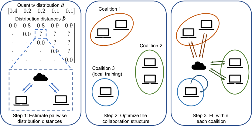
Figure 2: An overview of FedCollab

Quantifying the Quantity-Aware Function

The quantity-aware function $\phi_{|\mathcal{H}|}(\boldsymbol{\alpha}_{i},\boldsymbol{\beta},m,\delta)$ indicates the influence of data quantity. However, it is related to the complexity of hypothesis space $\mathcal{H}$, which can be hard to estimate accurately for neural networks. Inspired by earlier works on the model-complexity-based generalization bounds (Cao et al., 2019; Sagawa et al., 2020; Mohri & Medina, 2012), we treat the model capacity constant $C=\sqrt{2d\log(2m+2)+\log(4/\delta)}$ as a hyperparameter to tune. This gives the empirical quantity-aware function:

$$\hat{\phi}(\boldsymbol{\alpha}_{i},\boldsymbol{\beta},m,C)=\frac{C}{\sqrt{m}}\cdot\sqrt{\sum_{j=1}^{N}\frac{\alpha_{ij}^{2}}{\beta_{j}}}$$ (7)

Notice that $\boldsymbol{\beta}$ and $m$ can be directly calculated with the quantities reported by each client directly.

Quantifying the Distribution Differences

In Theorem 3.3, the distribution difference $D(\mathcal{D}_{i},\mathcal{D}_{j})$ is defined on two clients’ underlying distributions $\mathcal{D}_{i},\mathcal{D}_{j}$, which is typically not available in practice. Previous CFL algorithms (Sattler et al., 2021; Long et al., 2022) usually rely on the similarity of parameters/gradients, which indirectly reflect the distribution difference of clients. These methods are less accurate in the estimation of distribution distance, due to the non-convexity and permutation invariance of neural networks (Wang et al., 2020a). For example, even when we train two neural networks on two identical datasets, the parameters of two networks can vary significantly due to the differences in parameter initialization, the randomness of data loading, etc.

In domain adaptation, when estimating the distribution distance between two domains (distributions), a common practice is to train a domain discriminator (Ben-David et al., 2010) to predict which domain a randomly drawn sample is from. However, traditional domain adaptation requires putting data from two domains together, which violates the privacy constraints of FL. Therefore, we design an algorithm to estimate pairwise distribution difference between two clients without sharing their data. Notice that different from domain adaptation, our goal is to estimate the distribution difference, rather than aligning two distributions.

In particular, we use the $\mathcal{C}$-divergence to quantify the distribution differences, i.e.,

$$\begin{split}&D(\mathcal{D}_{i},\mathcal{D}_{j})=\max_{h\in\mathcal{H}}\left|\epsilon_{i}(h)-\epsilon_{j}(h)\right|=\\ &\max_{h\in\mathcal{H}}\left|\mathbb{E}_{(\boldsymbol{x},\boldsymbol{y})\in\mathcal{D}_{i}}\ell(h(\boldsymbol{x}),\boldsymbol{y})-\mathbb{E}_{(\boldsymbol{x},\boldsymbol{y})\in\mathcal{D}_{j}}\ell(h(\boldsymbol{x}),\boldsymbol{y})\right|\end{split}$$ (8)

where $\ell$ is the 0-1 loss. We can further rewrite $f(\boldsymbol{x},\boldsymbol{y})=\ell(h(\boldsymbol{x}),\boldsymbol{y})$ as a mapping $\mathcal{X}\times\mathcal{Y}\to\{0,1\}$. With detailed derivation provided in Appendix A.3, the equation above can be transformed as

$$\begin{split}&\max_{f\in\mathcal{F}}\left|\Pr_{(\boldsymbol{x},\boldsymbol{y})\in\mathcal{D}_{i}}[f(\boldsymbol{x},\boldsymbol{y})=1]+\Pr_{(\boldsymbol{x},\boldsymbol{y})\in\mathcal{D}_{j}}[f(\boldsymbol{x},\boldsymbol{y})=0]-1\right|\\ &=\max_{f\in\mathcal{F}}\left|2\cdot\text{BalAcc}(f,\{\mathcal{D}_{i},1\}\cup\{\mathcal{D}_{j},0\})-1\right|\end{split}$$

The equation above shows that we can train a client discriminator $f\in\mathcal{F}$ to predict 1, 0 on client $i,j$, respectively. The estimated distance is a simple function of the balanced accuracy (BalAcc) of the discriminator. Intuitively, when two distributions are distinctly different, a classifier will discriminate two distributions with BalAcc $\approx 100\%$, thus the distance $\approx 1$. Meanwhile, when two distributions are similar, the classifier cannot outperform random guessing, which results in BalAcc $\approx 50\%$ and thus the distance $\approx 0$.

Notice that while our FL model takes features $\boldsymbol{x}$ as input and predicts label, the client discriminator takes feature-label pairs $(\boldsymbol{x},\boldsymbol{y})$ as input and predicts sample origin. By taking feature-label pairs as input, the estimated $\mathcal{C}$-divergence can capture a wide range of distribution shifts, including feature shift (different $P(\boldsymbol{x})$), label shift (different $P(\boldsymbol{y})$), and concept shift (different $P(\boldsymbol{y}|\boldsymbol{x})$). In practice, we instantiate the client discriminator $f$ with a 2-layer neural network $f_{\boldsymbol{w}}$ with parameters $\boldsymbol{w}$, and train the client discriminator within FL framework, with pseudo-code in Algorithm 1. By using light-weight client discriminator, estimating pairwise distribution differences is much more efficient than training FL models. We quantify and compare their computation and communication complexities in Appendix B.4.

Algorithm 1 Training client discriminator

0:  Clients $i,j$ with local datasets $\hat{}\mathcal{D}_{i},\hat{}\mathcal{D}_{j}$, $m_{\text{train}},\boldsymbol{w}_{S}^{0},T$

0:  Distribution distance estimation $\hat{D}_{ij}$

1:  Train-valid split: $\hat{\mathcal{D}}_{i}=\hat{}\mathcal{D}_{i}^{\text{train}}\cup\hat{}\mathcal{D}_{i}^{\text{valid}},\hat{\mathcal{D}}_{j}=\hat{}\mathcal{D}_{j}^{\text{train}}\cup\hat{}\mathcal{D}_{j}^{\text{valid}}$ with $|\hat{}\mathcal{D}_{i}^{\text{train}}|=|\hat{}\mathcal{D}_{j}^{\text{train}}|=m_{\text{train}}$

2:  for communication round $t=1,\cdots,T$ do

3:     Server sends $\boldsymbol{w}_{S}^{t-1}$ to two clients

4:     for client $k\in\{i,j\}$ in parallel do

5:        Let client index $c=1,0$ for client $i,j$, respectively

6:        $\boldsymbol{w}_{k}^{t}\leftarrow\text{LocalUpdate}(\boldsymbol{w}_{S}^{t-1},\{\hat{}\mathcal{D}_{i}^{\text{train}},c\})$

7:        Client sends $\boldsymbol{w}_{k}^{t}$ to server

8:     end for

9:     $\boldsymbol{w}_{S}^{t}\leftarrow\frac{1}{2}(\boldsymbol{w}_{i}^{t}+\boldsymbol{w}_{j}^{t})$

10:  end for

11:  $\hat{D}_{ij}\leftarrow 2\cdot\text{BalAcc}(f_{\boldsymbol{w}_{S}^{T}},\{\mathcal{D}_{i}^{\text{valid}},1\}\cup\{\mathcal{D}_{j}^{\text{valid}},0\})-1$

Combining Error Bounds from All Clients

Finally, we combine the error bounds of all clients to form the following objective function. Given a collaboration structure $\{\mathcal{C}_{1},\cdots,\mathcal{C}_{K}\}$ with $K$ non-overlapping coalitions, where $K$ is an indeterminate number of coalitions, clients from the same coalition have the same collaboration vector $\boldsymbol{\alpha}_{i}$ as defined in Eq. (1) since they share the same global model. Here we define the collaboration matrix $\boldsymbol{A}=[\boldsymbol{\alpha}_{1}^{\top},\cdots,\boldsymbol{\alpha}_{N}^{\top}]^{\top}$ as follows.

$$\boldsymbol{A}_{ij}=\alpha_{ij}=\begin{cases}\frac{\beta_{j}}{\sum_{l\in\mathcal{C}_{k}}\beta_{l}},&\text{if }i\in\mathcal{C}_{k},j\in\mathcal{C}_{k},\exists k\\ 0,&\text{otherwise}\end{cases}$$ (9)

Then, the FedCollab objective can be formulated as

$$\begin{split}\mathcal{L}(\boldsymbol{A},\boldsymbol{\beta},m,\hat{}\boldsymbol{D})&=\sum_{i=1}^{N}\left(\frac{C}{\sqrt{m}}\sqrt{\sum_{j=1}^{N}\frac{\alpha_{ij}^{2}}{\beta_{j}}}+\sum_{j=1}^{N}\alpha_{ij}\hat{D}_{ij}\right)\\ &=\frac{C}{\sqrt{m}}\sum_{i=1}^{N}\|\boldsymbol{\alpha}_{i}\|_{\text{diag}(\boldsymbol{\beta})^{-1}}^{2}+\boldsymbol{A}\odot\hat{}\boldsymbol{D}\end{split}$$ (10)

where $\odot$ is the element-wise product. In the next part, we propose an efficient optimizer to find a collaboration structure that minimizes the objective above.

4.2 FedCollab Optimizer

Note that optimizing collaboration structure involves not only determining the objective but also how to optimize it. For example, while the objective is concise, constraints on $\boldsymbol{A}$ in Eq. (9) make optimization challenging: the range of $\boldsymbol{A}$ is discrete, and thus gradient descent cannot be directly used.

Therefore, we propose an efficient algorithm to solve the problem in discrete space. We optimize the coalition assignment $p(\cdot)$ which maps the client index to a coalition index (e.g., $p(1)=2$ means assigning client 1 to coalition 2). We initialize the coalition assignment with local training, i.e., $p(i)=i,\forall i$, and iteratively assign clients to a new coalition that can further minimize the FedCollab objective in Eq (10). Algorithm 2 gives the pseudo-code of the optimizer.

Algorithm 2 FedCollab optimizer

0:  $\boldsymbol{\beta},m,\hat{}\boldsymbol{D}$

0:  Coalition assignment $p(\cdot)$

1:  Initialize $p(i)=i$ for all clients (local training)

2:  while not converged do

3:     for client index $k$ in a permutation of $[1,\cdots,N]$ do

4:        Evaluate the objective of Eq. (10) with the new collaboration structure after setting $p(k)=1,\cdots,N$

5:        Update $p(k)$ to the coalition with lowest value of Eq. (10)

6:     end for

7:  end while

The optimizer guarantees to converge to local optimum, since the objective function has finite values and strictly decreases in each iteration. In practice, since greedy methods generally do not guarantee the global optimum, we re-run Algorithm 2 multiple times with different random seeds to further refine the collaboration structure. Different from most CFL algorithms (Ghosh et al., 2020; Long et al., 2022), where re-optimizing the collaboration structure requires re-training FL models and introduces large computation and communication costs, the collaboration optimization process of FedCollab is purely on the server and does not require training any ML model. As a result, our optimizer is very efficient and only takes a few seconds to run.

4.3 Training FL Models

After solving the collaboration structure, FedCollab fixes the collaboration and trains FL models within each coalition separately. Notice that since the collaboration structure and the FL model are optimized independently, FedCollab can be seamlessly integrated with any GFL or PFL algorithms in this stage.

4.4 New Training Clients

An additional advantage of FedCollab is that while typical cross-silo FL systems (Karimireddy et al., 2020; Smith et al., 2017) are expensive to allow new clients to join after the training of FL models, our FedCollab framework allows new clients to join a cross-silo FL system without the need for re-clustering and re-training all FL models. In particular, FedCollab assigns new clients to existing coalitions that minimize the objective in Eq. (10) by estimating the distribution distance between the new client and existing clients, thus requiring only one coalition to fine-tune or re-train the FL model for each new client.

5 Experiments

In this section, we design experiments to answer the following research questions:

• RQ1: Can FedCollab alleviate negative transfer for both GFL and PFL?

• RQ2: Can FedCollab provide better collaboration structures than previous CFL algorithms?

• RQ3 (hyperparameter): How do the choices of hyperparameter $C$ affect FedCollab?

• RQ4 (ablation study): How do different components contribute to the effectiveness of FedCollab?

• RQ5: Can FedCollab utilize new training clients? (see Appendix B.2)

• RQ6 (convergence): Does FedCollab optimizer converge efficiently and effectively? (see Appendix B.3)

Table 1: Alleviating negative transfer of base GFL and PFL algorithms with different models, datasets, and types of non-IIDness, where we report the mean and standard deviation for each evaluation metric in percentage ($\%$) after five runs.

Method	Label Shift (FashionMNIST)			Feature Shift (CIFAR-10)			Concept Shift (CIFAR-100)
	Acc $\uparrow$	IPR $\uparrow$	RSD $\downarrow$	Acc $\uparrow$	IPR $\uparrow$	RSD $\downarrow$	Acc $\uparrow$	IPR $\uparrow$	RSD $\downarrow$
Local Train	$86.05$ ($0.28$)	-	-	$38.65$ ($0.44$)	-	-	$29.82$ ($0.56$)	-	-
FedAvg	$46.64$ ($0.12$)	$46.00$ ($2.24$)	$41.03$ ($0.24$)	$44.31$ ($0.98$)	$86.00$ ($4.18$)	$4.62$ ($0.58$)	$26.62$ ($0.12$)	$50.00$ ($0.00$)	$11.54$ ($0.45$)
+FedCollab	$92.45$ ($0.07$)	$100.00$ ($0.00$)	$5.99$ ($0.41$)	$52.61$ ($0.60$)	$100.00$ ($0.00$)	$3.30$ ($0.63$)	$40.94$ ($0.22$)	$100.00$ ($0.00$)	$2.78$ ($0.30$)
FedProx	$46.70$ ($0.08$)	$45.00$ ($5.00$)	$41.09$ ($0.29$)	$44.45$ ($0.58$)	$87.00$ ($4.47$)	$4.74$ ($0.56$)	$26.78$ ($0.14$)	$50.00$ ($0.00$)	$11.66$ ($0.36$)
+FedCollab	$92.39$ ($0.15$)	$100.00$ ($0.00$)	$6.02$ ($0.37$)	$52.73$ ($0.64$)	$100.00$ ($0.00$)	$3.16$ ($0.61$)	$40.99$ ($0.17$)	$100.00$ ($0.00$)	$2.79$ ($0.34$)
FedNova	$75.92$ ($1.14$)	$45.00$ ($3.54$)	$12.38$ ($1.25$)	$46.98$ ($0.57$)	$99.00$ ($2.24$)	$3.42$ ($0.22$)	$26.46$ ($0.13$)	$50.00$ ($0.00$)	$10.57$ ($0.32$)
+FedCollab	$92.47$ ($0.13$)	$100.00$ ($0.00$)	$5.97$ ($0.39$)	$52.72$ ($0.57$)	$100.00$ ($0.00$)	$3.18$ ($0.63$)	$40.92$ ($0.36$)	$100.00$ ($0.00$)	$2.75$ ($0.43$)
Finetune	$67.32$ ($3.17$)	$48.00$ ($2.74$)	$22.97$ ($2.82$)	$44.17$ ($0.99$)	$82.00$ ($2.74$)	$5.14$ ($0.32$)	$33.30$ ($4.79$)	$50.00$ ($0.00$)	$13.95$ ($0.57$)
+FedCollab	$92.57$ ($0.15$)	$99.00$ ($2.24$)	$6.07$ ($0.30$)	$51.53$ ($0.61$)	$100.00$ ($0.00$)	$2.92$ ($0.46$)	$40.94$ ($2.36$)	$100.00$ ($0.00$)	$2.54$ ($0.30$)
Per-FedAvg	$51.13$ ($4.10$)	$49.00$ ($2.24$)	$37.35$ ($4.15$)	$43.78$ ($0.69$)	$83.00$ ($9.08$)	$4.74$ ($0.65$)	$27.39$ ($0.24$)	$50.00$ ($0.00$)	$12.24$ ($0.46$)
+FedCollab	$92.16$ ($0.25$)	$97.00$ ($6.71$)	$6.00$ ($0.25$)	$52.64$ ($0.45$)	$100.00$ ($0.00$)	$3.03$ ($0.30$)	$41.04$ ($0.26$)	$100.00$ ($0.00$)	$2.85$ ($0.49$)
pFedMe	$55.31$ ($3.45$)	$47.00$ ($4.47$)	$33.71$ ($3.11$)	$39.74$ ($0.85$)	$60.00$ ($12.25$)	$4.81$ ($0.74$)	$27.04$ ($0.39$)	$48.00$ ($2.74$)	$10.39$ ($0.47$)
+FedCollab	$92.18$ ($0.43$)	$99.00$ ($2.24$)	$6.40$ ($0.81$)	$47.20$ ($1.29$)	$97.00$ ($2.74$)	$3.02$ ($0.30$)	$37.47$ ($0.31$)	$100.00$ ($0.00$)	$3.04$ ($0.23$)
Ditto	$68.73$ ($1.40$)	$48.00$ ($2.74$)	$20.29$ ($2.06$)	$47.04$ ($0.30$)	$97.00$ ($2.74$)	$3.85$ ($0.35$)	$32.50$ ($0.40$)	$50.00$ ($0.00$)	$12.22$ ($0.36$)
+FedCollab	$92.55$ ($0.08$)	$99.00$ ($2.24$)	$6.11$ ($0.30$)	$50.97$ ($0.75$)	$99.00$ ($2.24$)	$3.38$ ($1.55$)	$40.33$ ($0.33$)	$100.00$ ($0.00$)	$2.16$ ($0.30$)

5.1 Setup

Models and Datasets

We evaluate our framework on three models and datasets: we train a 3-layer MLP for FashionMNIST (Xiao et al., 2017), a 5-layer CNN for CIFAR-10 (Krizhevsky, 2009), and an ImageNet pre-trained ResNet-18 (He et al., 2016) for CIFAR-100 (with 20 coarse labels). We simulate three typical scenarios of non-IIDness (Kairouz et al., 2021) on three datasets respectively, to show that our algorithm can handle a wide range of non-IIDness. For all scenarios, we simulate 20 clients with four types.

• Label shift (Ma et al., 2022). Each client has a different label distribution. Figure 3 visualizes the label and quantity distribution for each client. Different from Dirichlet partition (Hsu et al., 2019), where the distribution distance between any two clients has the same expectation, we create multiple levels of distribution distances. For example, client 0’s label distribution is most close to clients 1-4, less close to clients 5-9, and very distinct to clients 10-19.

• Feature shift (Ghosh et al., 2020). Each client’s image is rotated for a given angle: $+25^{\circ}$, $-25^{\circ}$, $+155^{\circ}$, $-155^{\circ}$ for clients 0-4, 5-9, 10-14, and 15-19, respectively. Multiple levels of distribution distances also exist in this scenario: client 0’s images have $0^{\circ}$ angle difference from client 1-4, $50^{\circ}$ from client 5-9, $130^{\circ}$ from client 10-14, and $180^{\circ}$ from client 15-19.

• Concept shift (Sattler et al., 2021). Each client’s label indices are permuted with the order given in Figure 4. Similar multiple levels of distribution distances are constructed: client 0 has all labels aligned with clients 1-4, 14 labels aligned with clients 5-9, and no label aligned with clients 10-19.

To simulate quantity shift while remaining explainability, we let clients 0-9 be “large” clients with more data, and clients 10-19 be “small” clients with less data. As a result, the large clients are more picky, and perform the best when they only collaborate with the same type of client (e.g., client 0 performs the best within a coalition of 0-4). However, small clients will prefer larger coalitions (e.g., client 10 performs the best within a coalition of 10-19).

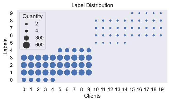
Figure 3: Label and quantity distributions for label shift scenario.

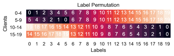
Figure 4: Label permutation for concept shift scenario.

Metrics

To comprehensively evaluate the FL algorithms, besides the accuracy score (Acc), we use incentivized participation rate (IPR) (Cho et al., 2022) to evaluate how many clients get accuracy gains compared to local training, and reward standard deviation (RSD) to evaluate the fairness of accuracy gains. Both metrics are defined with local model $\hat{h}_{i}^{\text{local}}$ and FL model $\hat{h}_{i}^{\text{FL}}$.

IPR $$=\frac{1}{N}\sum_{i=1}^{N}\mathbb{I}\{\text{acc}(\hat{h}_{i}^{\text{FL}})-\text{acc}(\hat{h}_{i}^{\text{local}})>0\}$$ (11)

RSD $$=\text{SD}(\{\text{acc}(\hat{h}_{i}^{\text{FL}})-\text{acc}(\hat{h}_{i}^{\text{local}})\}_{i=1}^{N})$$ (12)

where SD is the standard deviation. In an ideal FL system, all clients can get similar accuracy gains, which indicates a large IPR and small RSD.

For all three datasets, we use a light-weight two-layer MLP as the client discriminator to estimate pairwise distribution distances. For CIFAR-10/CIFAR-100, we use an ImageNet pre-trained ResNet-18 to encode the raw image to 512 dimensions as a pre-processing step, before feeding it into the client discriminator. Notice that since the parameters of the ResNet-18 encoder is not trained or transmitted, it does not introduce any additional communication cost.

Table 2: Comparison with Clustered FL

Method	Label Shift (FashionMNIST)			Feature Shift (CIFAR-10)			Concept Shift (CIFAR-100)
	Acc $\uparrow$	IPR $\uparrow$	RSD $\downarrow$	Acc $\uparrow$	IPR $\uparrow$	RSD $\downarrow$	Acc $\uparrow$	IPR $\uparrow$	RSD $\downarrow$
IFCA	$91.49$ ($0.61$)	$95.00$ ($5.00$)	$5.62$ ($0.54$)	$49.78$ ($1.01$)	$100.00$ ($0.00$)	$3.13$ ($0.52$)	$30.74$ ($4.46$)	$60.00$ ($22.36$)	$11.28$ ($5.04$)
FedCluster	$92.07$ ($0.47$)	$95.00$ ($7.07$)	$6.14$ ($0.49$)	$44.86$ ($1.90$)	$79.00$ ($17.10$)	$5.64$ ($1.81$)	$29.23$ ($2.18$)	$62.00$ ($12.55$)	$9.55$ ($0.69$)
FeSEM	$56.79$ ($6.71$)	$45.00$ ($11.18$)	$36.12$ ($2.08$)	$42.73$ ($0.37$)	$82.00$ ($5.70$)	$4.10$ ($0.62$)	$31.92$ ($3.12$)	$72.00$ ($12.55$)	$9.81$ ($1.77$)
KMeans	$69.30$ ($0.81$)	$72.00$ ($2.74$)	$35.87$ ($1.22$)	$48.61$ ($1.15$)	$96.00$ ($4.18$)	$4.54$ ($0.74$)	$34.24$ ($3.01$)	$85.00$ ($13.69$)	$6.47$ ($3.06$)
FedCollab	$92.45$ ($0.07$)	$100.00$ ($0.00$)	$5.99$ ($0.41$)	$52.61$ ($0.60$)	$100.00$ ($0.00$)	$3.30$ ($0.63$)	$40.94$ ($0.22$)	$100.00$ ($0.00$)	$2.78$ ($0.30$)

5.2 Alleviating Negative Transfer (RQ1)

We first show that while GFL and PFL algorithms suffer from negative transfer, after integrated with FedCollab, their negative transfer can be alleviated. We consider a wide range of SOTA GFL and PFL algorithms. For GFL, besides FedAvg (McMahan et al., 2017), we also compare to FedProx (Li et al., 2020a) (for better stability to non-IIDness) and FedNova (Wang et al., 2020b) (for more consistent objective under quantity shift). For PFL, we include Finetune (where each client locally finetunes the FedAvg model), a meta-learning-based method Per-FedAvg (Fallah et al., 2020), a regularization-based method pFedMe (Dinh et al., 2020), and a fair-and-robust method Ditto (Li et al., 2021).

We report the results in Table 1. Across datasets, models and types of non-IIDness, our proposed FedCollab strongly enhances the performance of all seven base FL algorithms in terms of accuracy, IPR and fairness (RSD). In the label shift and concept shift scenarios, all the base GFL and PFL algorithms strongly suffer from negative transfer: more than half of the clients (mostly the small clients) receive a FL model worse than local model. Although PFLs introduce accuracy gain compared to FedAvg, they do not solve the negative transfer problem since small clients still do not benefit from FL. However, when combined with our FedCollab, all base FL algorithms can reach a near $100\%$ IPR with much better accuracy and reward fairness.

In the feature shift scenarios, since rotation is a mild kind of non-IIDness also used for data augmentation, base FL algorithms suffer less from negative transfer compared to the other two scenarios: all the base FL algorithms get accuracy gain in average. Our FedCollab framework can further boost these FL algorithms to the next level, also reach a near $100\%$ IPR with significantly better accuracy and reward fairness.

It is also interesting to notice that after combining with our FedCollab framework, four PFL algorithms have limited or no accuracy gain compared to GFL algorithms. This enlightens us that “who to collaborate” may be more important than “how to collaborate”, and should be considered first.

5.3 Comparison to other CFL Algorithms (RQ2)

In this part, we compare our FedCollab algorithm (combined with FedAvg) to baseline CFL algorithms, including one loss-based algorithm IFCA (Ghosh et al., 2020), one gradient-based algorithm FedCluster (Sattler et al., 2021), and two parameter-based algorithms FeSEM (Long et al., 2022) and KMeans (Ghosh et al., 2019). We report the results in Table 2. Across all scenarios, FedCollab has the highest accuracy and IPR, with RSD among the lowest. Besides numerical results, we further study why FedCollab has better performance than baseline CFL methods.

Quantity Awareness

While FedCollab explicitly uses the quantity distribution $\boldsymbol{\beta}$ during collaboration optimization, all four baseline CFL algorithms cannot utilize the quantity information. For example, IFCA uses training losses to choose the model (cluster), which is not sensitive to the quantities. Therefore, it usually results in two clusters: 0-9 and 10-19, without further splitting the “large” clients.

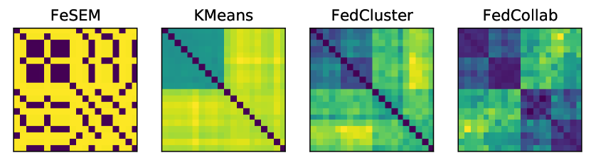
Figure 5: Client distance matrices on CIFAR-10 with feature shift.

Distribution Distances

Apart from the quantity awareness, our FedCollab framework estimates high-quality distribution distances. Notice that FeSEM and KMeans rely on the distance between model parameters, while FedCluster relies on gradient similarity matrix $\boldsymbol{S}$. We visualize the distance matrix of FedCollab and these baselines in Figure 5 (for FedCluster we show $1-\boldsymbol{S}$). It can be seen that the distance matrix of FeSEM is highly random depending on the initialization. KMeans gives some meaningful estimations, but the distance between two clients with the same underlying distribution is still high. While FedCluster gives the best estimation among baselines, the estimated distribution distance of FedCollab clearly reveals the multi-level distribution distances we construct.

Besides the performance, we also point out that while IFCA, FedCluster and FeSEM perform clustering during FL, KMeans and FedCollab perform clustering before FL. We compare these two types of CFL in Appendix B.5.

5.4 Effects of Hyperparameter (RQ3)

Our algorithm has a hyperparameter $C$ that balances generalization error and dataset shift. We study the effect of $C$ with results shown in Figure 6. When $C=6,8,10$, FedCollab gives the same collaboration structure with the highest accuracy. When we decrease $C$, the solved collaboration structure changes from coarse to fine, and finally to local training when $C=0$. On the other hand, when $C$ goes to infinity, the solved collaboration structure changes to global training, which suffers from negative transfer.

Figure 6: Effects of $C$ on FashionMNIST with label shift.

5.5 Ablation Study (RQ4)

In this part, we show that both distribution distances and quantity contribute to the optimization of collaboration structure. To this end, we consider two variants of FedCollab. With dataset untouched, “ignore quantities” replaces the real quantity distribution $\boldsymbol{\beta}$ with a uniform vector $\frac{1}{N}\boldsymbol{1}$, while “ignore distances” replaces the non-diagonal elements in the estimated distribution distance matrix $\hat{}\boldsymbol{D}$ with their average.

Table 3 summarizes the results of the ablation study. When ignoring distances, we observe that FedCollab assigns clients with no overlapping labels to the same coalition, which results in worse performance. When ignoring quantities, we observe that FedCollab forms multiple coalitions for small clients, instead of a large coalition for clients 10-19. Therefore, small clients get smaller performance gains compared to the original FedCollab.

Table 3: Ablation study on FashionMNIST with label shift

Method	Acc $\uparrow$	IPR $\uparrow$	RSD $\downarrow$
FedCollab	$92.45$ ($0.07$)	$100.00$ ($0.00$)	$5.99$ ($0.41$)
Ignore quantities	$90.31$ ($0.11$)	$94.00$ ($5.48$)	$4.30$ ($0.46$)
Ignore distances	$67.79$ ($0.89$)	$19.00$ ($4.18$)	$18.97$ ($0.83$)

6 Conclusion

We present FedCollab, a CFL framework that alleviates negative transfer in FL. Inspired by our derived generalization error bound for FL clients, FedCollab utilizes both quantity and distribution distance information to optimize the collaboration structure among clients. Extensive experiments demonstrate that FedCollab can boost the accuracy, incentivized participation rate and fairness of a wide range of GFL and PFL algorithms and a variety of non-IIDness. Moreover, FedCollab significantly outperforms state-of-the-art clustered FL algorithms in optimizing the collaboration structure among clients.

Appendix A Proofs

A.1 Proof of Theorem 3.3

In this part, we give the proof of Theorem 3.3. We first formally define the quantity-aware function $\phi_{|\mathcal{H}|}(\boldsymbol{\alpha}_{i},\boldsymbol{\beta},m,\delta)$ in Definition 3.1 and the distribution difference term $D(\mathcal{D}_{i},\mathcal{D}_{j})$ in Definition 3.2

A.1.1 Quantity-aware function

Definition 3.1 (Quantity-aware function).

For a given hypothesis space $\mathcal{H}$, fixed combination weights $\boldsymbol{\alpha}_{i}$, quantity distribution $\boldsymbol{\beta}$, total quantity $m$, for any $\delta\in(0,1)$, with probability at least $1-\delta$ (over the choice of the samples), the following holds for all $h\in\mathcal{H}$,

$$|\hat{\epsilon}_{\boldsymbol{\alpha}_{i}}(h)-\epsilon_{\boldsymbol{\alpha}_{i}}(h)|\leq\phi_{|\mathcal{H}|}(\boldsymbol{\alpha}_{i},\boldsymbol{\beta},m,\delta)$$ (13)

Remark A.1.

Definition 3.1 is an abstract form of the difference between $\epsilon_{\boldsymbol{\alpha}_{i}}(h)$, the expected loss on the mixture population distribution $\sum_{j=1}^{N}\alpha_{ij}\mathcal{D}_{j}$, and $\hat{\epsilon}_{\boldsymbol{\alpha}_{i}}(h)$, the empirical risk on finite samples drawn from the mixture empirical distribution $\sum_{j=1}^{N}\alpha_{ij}\hat{}\mathcal{D}_{j}$. It can be instantiated with traditional generalization error bounds. In the main text we give an example with VC dimension (Ben-David et al., 2010):

$$\phi_{|\mathcal{H}|}^{\text{VC}}(\boldsymbol{\alpha}_{i},\boldsymbol{\beta},m,\delta)=\sqrt{\left(\sum_{j=1}^{N}\frac{\alpha_{ij}^{2}}{\boldsymbol{\beta}_{j}}\right)\left(\frac{2d\log(2m+2)+\log(4/\delta)}{m}\right)}$$ (14)

Another choice is using weighted Rademacher complexity (Liu et al., 2015), which gives a similar form of the bound.

$$\phi_{|\mathcal{H}|}^{\text{Rad}}(\boldsymbol{\alpha}_{i},\boldsymbol{\beta},m,\delta)=\hat{R}_{\boldsymbol{\alpha}_{i}}(\mathcal{H})+3\sqrt{\frac{m}{2}\left(\max_{1\leq j\leq N}\frac{\alpha_{ij}}{m_{i}}\right)^{2}\log\left(\frac{2}{\delta}\right)}$$ (15)

where

$$\hat{R}_{\boldsymbol{\alpha}_{i}}(\mathcal{H})=\mathbb{E}_{\boldsymbol{\sigma}\in\{\pm 1\}^{m}}\sup_{h\in\mathcal{H}}2\sum_{j=1}^{N}\frac{\alpha_{ij}}{m_{j}}\sum_{k=1}^{m_{i}}\sigma_{j,k}\ell(h(\boldsymbol{x}_{k}^{(j)}),\boldsymbol{y}_{k}^{(j)})$$ (16)

It can be transformed into a similar form. Denote $\hat{R}_{j}(\mathcal{H})=\mathbb{E}_{\boldsymbol{\sigma}_{j}\in\{\pm 1\}^{m_{j}}}\sup_{h\in\mathcal{H}}2\sum_{k=1}^{m_{i}}\sigma_{j,k}\ell(h(\boldsymbol{x}_{k}^{(j)}),\boldsymbol{y}_{k}^{(j)})$ be the empirical Rademacher complexity of client $j$ with order $\mathcal{O}(\frac{1}{\sqrt{m_{j}}})$ (Shalev-Shwartz & Ben-David, 2014), we have

$$\hat{R}_{\boldsymbol{\alpha}_{i}}(\mathcal{H}) \leq\sum_{j=1}^{N}\alpha_{ij}\hat{R}_{j}(\mathcal{H})\leq\sqrt{N\sum_{j=1}^{N}\alpha_{ij}^{2}(\hat{R}_{j}(\mathcal{H}))^{2}}\leq\sqrt{N\sum_{j=1}^{N}\alpha_{ij}^{2}\cdot\left(\frac{C}{\sqrt{m_{j}}}\right)^{2}}=\sqrt{\left(\sum_{j=1}^{N}\frac{\alpha_{ij}^{2}}{\boldsymbol{\beta}_{j}}\right)\cdot\frac{NC^{2}}{m}},\quad\exists C>0$$ (17)

A.1.2 Distribution differences

Definition 3.2 (Distribution differences).

For a given hypothesis space $\mathcal{H}$, two distributions $\mathcal{D}_{i},\mathcal{D}_{j}$, the following holds for all $h\in\mathcal{H}$,

$$|\epsilon_{i}(h)-\epsilon_{j}(h)|\leq D(\mathcal{D}_{i},\mathcal{D}_{j})$$ (18)

Remark A.2.

Definition 3.2 also can be instantiated with different distribution distances. In the main text we focus on $\mathcal{C}$-divergence (Mohri & Medina, 2012; Wu & He, 2020), which utilizes both feature and label information.

$$D^{\mathcal{C}}(\mathcal{D}_{i},\mathcal{D}_{j})=\max_{h\in\mathcal{H}}|\epsilon_{i}(h)-\epsilon_{j}(h)|$$ (19)

Another common choice is using $\mathcal{H}\Delta\mathcal{H}$-distance (Ben-David et al., 2010). Denote $\mathcal{X}_{i},\mathcal{X}_{j}$ as the marginal feature distributions of $\mathcal{D}_{i},\mathcal{D}_{j}$, respectively,

$$D^{\mathcal{H}\Delta\mathcal{H}}(\mathcal{D}_{i},\mathcal{D}_{j})=\frac{1}{2}d_{\mathcal{H}\Delta\mathcal{H}}(\mathcal{X}_{i},\mathcal{X}_{j})+\lambda_{ij}$$ (20)

where $\lambda_{ij}=\min_{h\in\mathcal{H}}(\epsilon_{i}(h)+\epsilon_{j}(h))$ is assumed to be small and $d_{\mathcal{H}\Delta\mathcal{H}}(\mathcal{X}_{i},\mathcal{X}_{j})$ can be estimated with a client discriminator using only feature as input.

A.1.3 Error Upper Bound

Lemma A.3 (Error decomposition).

For all $h\in\mathcal{H}$, denote $\epsilon_{\boldsymbol{\alpha}_{i}}(h)=\sum_{j=1}^{N}\alpha_{ij}\epsilon_{\alpha_{j}}(h)$,

$$\left|\epsilon_{i}(h)-\epsilon_{\boldsymbol{\alpha}_{i}}(h)\right| =\left|\sum_{j=1}^{N}\alpha_{ij}\epsilon_{i}(h)-\sum_{j=1}^{N}\alpha_{ij}\epsilon_{j}(h)\right|$$

$$\leq\sum_{j\neq i}\alpha_{ij}\left|\epsilon_{i}(h)-\epsilon_{j}(h)\right|$$

$$\leq\sum_{j\neq i}\alpha_{ij}D(\mathcal{D}_{i},\mathcal{D}_{j})$$ (Definition 3.2)

Theorem 3.3.

Let $\hat{h}_{\boldsymbol{\alpha}_{i}}$ be the empirical risk minimizer defined in Eq. (1) and $h_{i}^{*}$ be client $i$’s expected risk minimizer. For any $\delta\in(0,\frac{1}{2})$, with probability at least $1-2\delta$, the following holds

$$\epsilon_{i}(\hat{h}_{\boldsymbol{\alpha}_{i}})\leq\epsilon_{i}(h_{i}^{*}) +2\phi_{|\mathcal{H}|}(\boldsymbol{\alpha}_{i},\boldsymbol{\beta},m,\delta)+2\sum_{j\neq i}\alpha_{ij}D(\mathcal{D}_{i},\mathcal{D}_{j})$$ (21)

Proof.

$$\epsilon_{i}(\hat{h}_{\boldsymbol{\alpha}_{i}}) \leq\epsilon_{\boldsymbol{\alpha}_{i}}(\hat{h}_{\boldsymbol{\alpha}_{i}})+\left|\epsilon_{\boldsymbol{\alpha}_{i}}(\hat{h}_{\boldsymbol{\alpha}_{i}})-\epsilon_{i}(\hat{h}_{\boldsymbol{\alpha}_{i}})\right|$$

$$\leq\epsilon_{\boldsymbol{\alpha}_{i}}(\hat{h}_{\boldsymbol{\alpha}_{i}})+\sum_{j\neq i}\alpha_{ij}D(\mathcal{D}_{i},\mathcal{D}_{j})$$ (Lemma A.3)

$$\leq\hat{\epsilon}_{\boldsymbol{\alpha}_{i}}(\hat{h}_{\boldsymbol{\alpha}_{i}})+\left|\epsilon_{\boldsymbol{\alpha}_{i}}(\hat{h}_{\boldsymbol{\alpha}_{i}})-\hat{\epsilon}_{\boldsymbol{\alpha}_{i}}(\hat{h}_{\boldsymbol{\alpha}_{i}})\right|+\sum_{j\neq i}\alpha_{ij}D(\mathcal{D}_{i},\mathcal{D}_{j})$$

$$\leq\hat{\epsilon}_{\boldsymbol{\alpha}_{i}}(\hat{h}_{\boldsymbol{\alpha}_{i}})+\phi_{|\mathcal{H}|}(\boldsymbol{\alpha}_{i},\boldsymbol{\beta},m,\delta)+\sum_{j\neq i}\alpha_{ij}D(\mathcal{D}_{i},\mathcal{D}_{j}) 1-\delta$$ (Definition 3.1, hold with probability )

$$\leq\hat{\epsilon}_{\boldsymbol{\alpha}_{i}}(h_{i}^{*})+\phi_{|\mathcal{H}|}(\boldsymbol{\alpha}_{i},\boldsymbol{\beta},m,\delta)+\sum_{j\neq i}\alpha_{ij}D(\mathcal{D}_{i},\mathcal{D}_{j})$$ (Empirical Minimizer)

$$\leq\epsilon_{\boldsymbol{\alpha}_{i}}(h_{i}^{*})+\left|\epsilon_{\boldsymbol{\alpha}_{i}}(h_{i}^{*})-\hat{\epsilon}_{\boldsymbol{\alpha}_{i}}(h_{i}^{*})\right|+\phi_{|\mathcal{H}|}(\boldsymbol{\alpha}_{i},\boldsymbol{\beta},m,\delta)+\sum_{j\neq i}\alpha_{ij}D(\mathcal{D}_{i},\mathcal{D}_{j})$$

$$\leq\epsilon_{\boldsymbol{\alpha}_{i}}(h_{i}^{*})+2\phi_{|\mathcal{H}|}(\boldsymbol{\alpha}_{i},\boldsymbol{\beta},m,\delta)+\sum_{j\neq i}\alpha_{ij}D(\mathcal{D}_{i},\mathcal{D}_{j}) 1-\delta$$ (Definition 3.1, hold with probability )

$$\leq\epsilon_{i}(h_{i}^{*})+\left|\epsilon_{i}(h_{i}^{*})-\epsilon_{\boldsymbol{\alpha}_{i}}(h_{i}^{*})\right|+2\phi_{|\mathcal{H}|}(\boldsymbol{\alpha}_{i},\boldsymbol{\beta},m,\delta)+\sum_{j\neq i}\alpha_{ij}D(\mathcal{D}_{i},\mathcal{D}_{j})$$

$$\leq\epsilon_{i}(h_{i}^{*})+2\phi_{|\mathcal{H}|}(\boldsymbol{\alpha}_{i},\boldsymbol{\beta},m,\delta)+2\sum_{j\neq i}\alpha_{ij}D(\mathcal{D}_{i},\mathcal{D}_{j})$$ (Lemma A.3)

Notice that we use the generalization error bound twice, so the bound holds with probability at least $1-2\delta$ instead of $1-\delta$. ∎

A.2 Proof of Corollaries 3.4 and 3.5

A.2.1 Proof of Corollary 3.4(1)

Corollary 3.4 (1).

When using VC-dimension bound (14) as the quantity aware function, if $D(\mathcal{D}_{i},\mathcal{D}_{j})=0,\forall i,j$, GFL minimizes the error bound with $\alpha_{ij}=\beta_{j},\forall{j}$.

Proof.

In the first case, $D(\mathcal{D}_{i},\mathcal{D}_{j})=0$. Let $Q=\sqrt{\frac{2d\log(2m+2)+\log(4/\delta)}{m}}$. Then

$$f(\boldsymbol{\alpha}_{i}) =2\phi_{|\mathcal{H}|}(\boldsymbol{\alpha}_{i},\boldsymbol{\beta},m,\delta)=2Q\sqrt{\sum_{j=1}^{N}\frac{\alpha_{ij}^{2}}{\beta_{j}}}$$

$$=2Q\sqrt{\sum_{j=1}^{N}\frac{(\alpha_{ij}-\beta_{j})^{2}}{\beta_{j}}+1}$$

$$=2Q\sqrt{\chi^{2}\left(\boldsymbol{\alpha}_{i}||\boldsymbol{\beta}\right)+1}$$

which achieves the minimum at $\boldsymbol{\alpha}_{i}=\boldsymbol{\beta}$. ∎

A.2.2 Proof of Corollary 3.5 and 3.4(2)

Corollary 3.5.

When using VC-dimension bound (14) as the quantity aware function, for a client $i$ with $m_{i}$ samples, if its coalition $\mathcal{C}$ minimizes the error bound of Theorem 3.3, then $\mathcal{C}$ does not include any clients with distribution distance $D(\mathcal{D}_{i},\mathcal{D}_{j})>D_{\text{thr}}$, where $D_{\text{thr}}=\frac{\sqrt{2d\log(2m+2)+\log(4/\delta)}\sqrt{m}}{2m_{i}}$.

Proof.

For the coalition $\mathcal{C}$, if there is at least one client $j\in\mathcal{C}$ with $\mathcal{D}(\mathcal{D}_{i},\mathcal{D}_{j})>D_{\text{thr}}>0$, we show that there exists a different coalition $\mathcal{C}^{-}=\{k\in\mathcal{C}:\mathcal{D}(\mathcal{D}_{i},\mathcal{D}_{k})\leq D_{\text{thr}}\}$ with strictly smaller error bound.

We denote $\mathcal{C}^{+}=\{k\in\mathcal{C},k\neq i:\mathcal{D}(\mathcal{D}_{i},\mathcal{D}_{k})>D_{\text{thr}}\}$ as the clients in the coalition with distribution differences strictly larger than $D_{\text{thr}}$, and $\mathcal{C}^{-}=\{k\in\mathcal{C},k\neq i:\mathcal{D}(\mathcal{D}_{i},\mathcal{D}_{k})\leq D_{\text{thr}}\}\cup\{i\}$ as the clients in the coalition with distribution differences smaller than or equal to $D_{\text{thr}}$ (including client $i$ itself). Notice that

• $\mathcal{C}=\mathcal{C}^{+}\cup\mathcal{C}^{-}$,

• $\mathcal{C}^{-}\subsetneqq\mathcal{C},\mathcal{C}^{+}\neq\emptyset$, and

• $i\in\mathcal{C}^{-}$.

Therefore, $\mathcal{C}^{-}$ is a different coalition for client $i$. Next, we prove that coalition $\mathcal{C}^{-}$ has a strictly smaller error bound than $\mathcal{C}$. For clarity, we denote $m_{\mathcal{C}}=\sum_{j\in\mathcal{C}}m_{j}$ and $\mu=\sqrt{2d\log(2m+2)+\log(4/\delta)}$. We first quantify the error bound for $\mathcal{C}$.

$$\text{error\_bound}(\mathcal{C}) =\epsilon_{i}(h_{i}^{*})+2\mu\sqrt{\frac{1}{m}\sum_{j\neq i}\frac{\alpha_{ij}^{2}}{\beta_{j}}}+2\sum_{j\neq i}\alpha_{ij}D(\mathcal{D}_{i},\mathcal{D}_{j})$$

$$=\epsilon_{i}(h_{i}^{*})+2\mu\sqrt{\frac{1}{m}\sum_{j\in\mathcal{C}}\frac{\left(\frac{\beta_{j}}{\sum_{k\in\mathcal{C}}\beta_{k}}\right)^{2}}{\beta_{j}}}+2\sum_{j\in\mathcal{C}-\{i\}}\frac{\beta_{j}}{\sum_{k\in\mathcal{C}}\beta_{k}}D(\mathcal{D}_{i},\mathcal{D}_{j})$$

$$=\epsilon_{i}(h_{i}^{*})+2\mu\sqrt{\frac{1}{m}\sum_{j\in\mathcal{C}}\frac{\beta_{j}}{\left(\sum_{k\in\mathcal{C}}\beta_{k}\right)^{2}}}+2\sum_{j\in\mathcal{C}-\{i\}}\frac{\beta_{j}}{\sum_{k\in\mathcal{C}-\{i\}}\beta_{k}}D(\mathcal{D}_{i},\mathcal{D}_{j})$$

$$=\epsilon_{i}(h_{i}^{*})+2\mu\sqrt{\frac{1}{\sum_{j\in\mathcal{C}}m_{j}}}+2\sum_{j\in\mathcal{C}-\{i\}}\frac{m_{j}}{\sum_{k\in\mathcal{C}}m_{k}}D(\mathcal{D}_{i},\mathcal{D}_{j})$$

$$=\epsilon_{i}(h_{i}^{*})+2\mu\sqrt{\frac{1}{m_{\mathcal{C}}}}+2\sum_{j\in\mathcal{C}-\{i\}}\frac{m_{j}}{m_{\mathcal{C}}}D(\mathcal{D}_{i},\mathcal{D}_{j})$$

We can quantify the error bound for $\mathcal{C}^{-}$ through the same steps. Then we can compare two error bounds.

$$\quad\ \ \text{error\_bound}(\mathcal{C})-\text{error\_bound}(\mathcal{C}^{-})$$

$$=\left(2\mu\sqrt{\frac{1}{m_{\mathcal{C}}}}+2\sum_{j\in\mathcal{C}-\{i\}}\frac{m_{j}}{m_{\mathcal{C}}}D(\mathcal{D}_{i},\mathcal{D}_{j})\right)-\left(2\mu\sqrt{\frac{1}{m_{\mathcal{C}^{-}}}}+2\sum_{j\in\mathcal{C}^{-}-\{i\}}\frac{m_{j}}{m_{\mathcal{C}^{-}}}D(\mathcal{D}_{i},\mathcal{D}_{j})\right)$$

$$=-2\mu\left(\sqrt{\frac{1}{m_{\mathcal{C}^{-}}}}-\sqrt{\frac{1}{m_{\mathcal{C}}}}\right)+2\left(\sum_{j\in\mathcal{C}-\{i\}}\frac{m_{j}}{m_{\mathcal{C}}}D(\mathcal{D}_{i},\mathcal{D}_{j})-\sum_{j\in\mathcal{C}^{-}-\{i\}}\frac{m_{j}}{m_{\mathcal{C}^{-}}}D(\mathcal{D}_{i},\mathcal{D}_{j})\right)$$

In the first term,

$$\sqrt{\frac{1}{m_{\mathcal{C}^{-}}}}-\sqrt{\frac{1}{m_{\mathcal{C}}}} =\frac{\frac{1}{m_{\mathcal{C}^{-}}}-\frac{1}{m_{\mathcal{C}}}}{\sqrt{\frac{1}{m_{\mathcal{C}^{-}}}}+\sqrt{\frac{1}{m_{\mathcal{C}}}}}$$

$$<\frac{\frac{1}{m_{\mathcal{C}^{-}}}-\frac{1}{m_{\mathcal{C}}}}{\sqrt{\frac{1}{m}}+\sqrt{\frac{1}{m}}}$$

$$=\frac{\sqrt{m}}{2}\left(\frac{1}{m_{\mathcal{C}^{-}}}-\frac{1}{m_{\mathcal{C}}}\right)$$

In the second term,

$$\quad\sum_{j\in\mathcal{C}-\{i\}}\frac{m_{j}}{m_{\mathcal{C}}}D(\mathcal{D}_{i},\mathcal{D}_{j})-\sum_{j\in\mathcal{C}^{-}-\{i\}}\frac{m_{j}}{m_{\mathcal{C}^{-}}}D(\mathcal{D}_{i},\mathcal{D}_{j})$$

$$=\sum_{j\in\mathcal{C}^{-}-\{i\}}\left(\frac{m_{j}}{m_{\mathcal{C}}}-\frac{m_{j}}{m_{\mathcal{C}^{-}}}\right)D(\mathcal{D}_{i},\mathcal{D}_{j})+\sum_{j\in\mathcal{C}^{+}}\frac{m_{j}}{m_{\mathcal{C}}}D(\mathcal{D}_{i},\mathcal{D}_{j})$$

$$>\sum_{j\in\mathcal{C}^{-}-\{i\}}\left(\frac{m_{j}}{m_{\mathcal{C}}}-\frac{m_{j}}{m_{\mathcal{C}^{-}}}\right)D_{\text{thr}}+\sum_{j\in\mathcal{C}^{+}}\frac{m_{j}}{m_{\mathcal{C}}}D_{\text{thr}}$$

$$=\left(\sum_{j\in\mathcal{C}-\{i\}}\frac{m_{j}}{m_{\mathcal{C}}}-\sum_{j\in\mathcal{C}^{-}-\{i\}}\frac{m_{j}}{m_{\mathcal{C}}^{-}}\right)D_{\text{thr}}$$

$$=\left(\frac{1}{m_{\mathcal{C}}^{-}}-\frac{1}{m_{\mathcal{C}}}\right)m_{i}D_{\text{thr}}$$

Put them together, we have

$$\text{error\_bound}(\mathcal{C})-\text{error\_bound}(\mathcal{C}^{-}) >-2\mu\frac{\sqrt{m}}{2}\left(\frac{1}{m_{\mathcal{C}^{-}}}-\frac{1}{m_{\mathcal{C}}}\right)+2\left(\frac{1}{m_{\mathcal{C}}^{-}}-\frac{1}{m_{\mathcal{C}}}\right)m_{i}D_{\text{thr}}$$

$$=\left(\frac{1}{m_{\mathcal{C}^{-}}}-\frac{1}{m_{\mathcal{C}}}\right)\left(2m_{i}D_{\text{thr}}-\mu\sqrt{m}\right)$$

$$=0$$

Therefore, the coalition $\mathcal{C}^{-}$ has a strictly smaller error bound than $\mathcal{C}$. ∎

Corollary 3.4 (2).

When using VC-dimension bound (14) as the quantity aware function, if $\min_{j\neq i}D(\mathcal{D}_{i},\mathcal{D}_{j})>\frac{\sqrt{2d\log(2m+2)+\log(4/\delta)}\sqrt{m}}{2m_{i}}$, where $d$ is the VC-dimension of the hypothesis space, local training minimizes the error bound with $\alpha_{ii}=1$ and $\alpha_{ij}=0,\forall j\neq i$.

Proof.

It is a special case for Corollary 3.5. Since $\forall i\neq j,D(\mathcal{D}_{i},\mathcal{D}_{j})>\frac{\sqrt{2d\log(2m+2)+\log(4/\delta)}\sqrt{m}}{2m_{i}}$, each client’s coalition should only include itself, which results in local training. ∎

A.3 Derivation of Client Discriminator

$$D(\mathcal{D}_{i},\mathcal{D}_{j}) =\max_{h\in\mathcal{H}}|\epsilon_{i}(h)-\epsilon(h)|$$

$$=\max_{h\in\mathcal{H}}\left|\mathbb{E}_{(\boldsymbol{x},\boldsymbol{y})\in\mathcal{D}_{i}}\ell(h(\boldsymbol{x}),\boldsymbol{y})-\mathbb{E}_{(\boldsymbol{x},\boldsymbol{y})\in\mathcal{D}_{j}}\ell(h(\boldsymbol{x}),\boldsymbol{y})\right|$$

$$=\max_{f\in\mathcal{F}}\left|\mathbb{E}_{(\boldsymbol{x},\boldsymbol{y})\in\mathcal{D}_{i}}f(\boldsymbol{x},\boldsymbol{y})-\mathbb{E}_{(\boldsymbol{x},\boldsymbol{y})\in\mathcal{D}_{j}}f(\boldsymbol{x},\boldsymbol{y})\right|$$

$$=\max_{f\in\mathcal{F}}\left|\Pr_{(\boldsymbol{x},\boldsymbol{y})\in\mathcal{D}_{i}}[f(\boldsymbol{x},\boldsymbol{y})=1]-\Pr_{(\boldsymbol{x},\boldsymbol{y})\in\mathcal{D}_{j}}[f(\boldsymbol{x},\boldsymbol{y})=1]\right|$$

$$=\max_{f\in\mathcal{F}}\left|\Pr_{(\boldsymbol{x},\boldsymbol{y})\in\mathcal{D}_{i}}[f(\boldsymbol{x},\boldsymbol{y})=1]+\Pr_{(\boldsymbol{x},\boldsymbol{y})\in\mathcal{D}_{j}}[f(\boldsymbol{x},\boldsymbol{y})=0]-1\right|$$

$$=\max_{f\in\mathcal{F}}\left|2\cdot\text{BalAcc}(f,\{\mathcal{D}_{i},1\}\cup\{\mathcal{D}_{j},0\})-1\right|$$

where

$$\text{BalAcc}(f,\{\mathcal{D}_{i},1\}\cup\{\mathcal{D}_{j},0\})=\frac{1}{2}\left(\Pr_{(\boldsymbol{x},\boldsymbol{y})\in\mathcal{D}_{i}}[f(\boldsymbol{x},\boldsymbol{y})=1]+\Pr_{(\boldsymbol{x},\boldsymbol{y})\in\mathcal{D}_{j}}[f(\boldsymbol{x},\boldsymbol{y})=0]\right)$$

is the balanced accuracy.

Appendix B Additional Experiments

B.1 Setup

Here we provide more information on our experimental settings. Table 4 show the statistics of training/testing samples in three scenarios we consider. Notice that the testing data is NOT used during collaboration structure optimization or FL model training.

Table 4: Number of training / testing samples on each client

Client	Label Shift (FashionMNIST)	Feature Shift (CIFAR-10)	Concept Shift (CIFAR-100)
“Large” (0-9)	2,100 / 350	2,500 / 500	2,500 / 500
“Small” (10-19)	14 / 350	340 / 500	120 / 500

We run $C=6,8,10$ on all three settings, and report the best result. Finally, we choose $C=10$ for FashionMNIST and CIFAR-10 experiments, and $C=8$ for CIFAR-100 experiments.

Our code is available at https://github.com/baowenxuan/FedCollab.

B.2 New Training Clients (RQ5)

In this part, we study whether new training clients can contribute to the FL system with a collaboration structure solved by FedCollab. We initialize a FedAvg system with 19 clients, leaving client 0 out. Client 0 operates local training in the first 200 rounds, and joins the FL system after 200 rounds (when FL models nearly converge). We use FedCollab to decide which coalition it should join. As shown in Figure 7, client 0 (“new”) receives a FL model with higher accuracy than the local model. Meanwhile, clients in the updated coalition (“clustered”) also benefit from the new training client since the FL model has additional performance gain after the new client 0 joins the training.

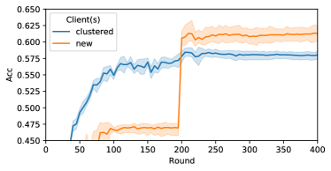
Figure 7: Utilizing new training clients on CIFAR-10 with feature shift

B.3 Convergence of FedCollab solver (RQ6)

Algorithm 2 is theoretically guaranteed to converge. In this part, we further study how many iterations it needs to converge, and whether it falls into local optima. Figure 8 visualizes the result of convergence. We re-run the FedCollab solver 100 times with different random seeds, and plot all trajectories indicating how the FedCollab loss changes w.r.t. inner iterations (line 3-6 in Algorithm 2). Notice that the FedCollab loss is evaluated for $N=20$ times in each inner iteration.

All the random runs converge within the first 60 inner iterations, while stopping within the first 80 inner iterations (since it requires one additional outer iteration to confirm convergence). Since the evaluation of FedCollab loss is very efficient, it only takes around 100ms to run Algorithm 2 once.

We also notice that a single run of Algorithm 2 cannot guarantee the optimal solution. In many runs, FedCollab solver converges to a sub-optimal solution, which gives a collaboration structure of [[0..4], [5..9], [10..14], [15..19]]. Therefore, we use multiple random runs to refine the collaboration structure.

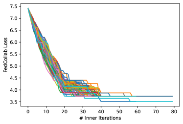
(a) # inner iteration v.s. loss value

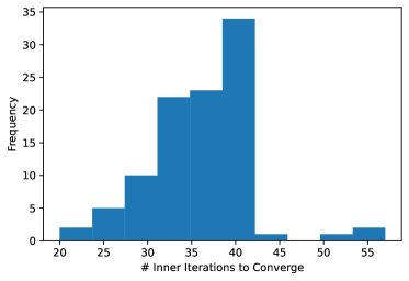
(b) Histogram of # inner iteration to converge

Figure 8: Convergence of Algorithm 2 on CIFAR-10

B.4 Computation and Communication Complexity

During the clustering step, FedCollab trains $\frac{N(N-1)}{2}$ client discriminators for $N$ clients, introducing $\mathcal{O}(N^{2})$ complexity. The complexity of FedCollab has the same order as many cross-silo FL algorithms, including MOCHA (Smith et al., 2017), FedFOMO (Zhang et al., 2021), and PACFL (Vahidian et al., 2022), which all model pairwise relationship among clients. Meanwhile, the training of client discriminators can be conducted in parallel: each client can train $N-1$ discriminators in parallel with other clients.

Table 5: Comparison of computation and communication complexities (CIFAR-100 experiment)

Model	MACs	Params
Client discriminator (MLP)	104,600	105,001
FL model (ResNet-18)	37,220,352	11,181,642

In the paper, to reduce the computation and communication constraints, we use a lightweight 2-layer MLP as the client discriminator, which is very efficient compared to the FL model (ResNet-18). We numerically evaluate their computation and communication complexities in the CIFAR-100 experiment.

• For computation cost, we count the number of multiply-add cumulations (MACs) for the forward pass of a single data point.

• For communication cost, we count the number of parameters (Params).

As shown in Table 5, the MACs and Params for client discriminator are negligible compared to the FL model. Considering that each client needs to train $N-1=19$ client discriminators in total, our clustering step still only introduces $\sim 5.3\%$ additional computation cost and $\sim 17.8\%$ additional communication cost for each client.

B.5 Discussion of Clustering During or before FL

Compared to clustering during FL, clustering before FL has the following advantages.

• Clustering before FL is more stable and efficient. IFCA and FeSEM conduct clustering during FL. Their clustering results are influenced by the random initialization, and can easily converge to suboptima. To jump out of local optima, IFCA must conduct the whole FL training for multiple times, which is very inefficient. In comparison, FedCollab does not rely on any random initialization of the collaboration structure, and can refine the collaboration structure within only a few seconds.

• Clustering before FL is more flexible. For clustering before FL, the clustering and FL phases are disentangled, which allows them to be seamlessly integrated with any GFL or PFL algorithms. Meanwhile, the convergence of clustering during FL algorithms may depend on specific FL algorithm.

• Clustering before FL saves communication cost for outliers. For outlier clients that have significantly different distribution from all other clients, FedCollab allows them to form self-clusters, and they do not need to participate in the FL phase anymore (see blue cluster in Figure 2). It saves communication cost for these outlier clients and the server. It also prevents other clients from being negatively affected by outlier clients.

For disadvantages, clustering before FL requires each client’s data set to be stable. In other words, the same client data set is used for clustering and FL. If the data sets for clustering and FL have different distributions or quantities, the optimal collaboration during clustering may not also be optimal for FL. However, this requirement is automatically satisfied for clustering during FL.

References

- Ben-David et al. (2010) Ben-David, S., Blitzer, J., Crammer, K., Kulesza, A., Pereira, F., and Vaughan, J. W. A theory of learning from different domains. Machine learning, 79(1):151–175, 2010.
- Caldas et al. (2018) Caldas, S., Wu, P., Li, T., Konečný, J., McMahan, H. B., Smith, V., and Talwalkar, A. LEAF: A benchmark for federated settings. CoRR, abs/1812.01097, 2018.
- Cao et al. (2019) Cao, K., Wei, C., Gaidon, A., Aréchiga, N., and Ma, T. Learning imbalanced datasets with label-distribution-aware margin loss. In Advances in Neural Information Processing Systems, pp. 1565–1576, 2019.
- Cho et al. (2022) Cho, Y. J., Jhunjhunwala, D., Li, T., Smith, V., and Joshi, G. To federate or not to federate: Incentivizing client participation in federated learning. CoRR, abs/2205.14840, 2022.
- Dinh et al. (2020) Dinh, C. T., Tran, N. H., and Nguyen, T. D. Personalized federated learning with moreau envelopes. In Advances in Neural Information Processing Systems, 2020.
- Donahue & Kleinberg (2021) Donahue, K. and Kleinberg, J. M. Model-sharing games: Analyzing federated learning under voluntary participation. In Thirty-Fifth AAAI Conference on Artificial Intelligence, pp. 5303–5311, 2021.
- Fallah et al. (2020) Fallah, A., Mokhtari, A., and Ozdaglar, A. E. Personalized federated learning with theoretical guarantees: A model-agnostic meta-learning approach. In Advances in Neural Information Processing Systems, 2020.
- Ghosh et al. (2019) Ghosh, A., Hong, J., Yin, D., and Ramchandran, K. Robust federated learning in a heterogeneous environment. CoRR, abs/1906.06629, 2019.
- Ghosh et al. (2020) Ghosh, A., Chung, J., Yin, D., and Ramchandran, K. An efficient framework for clustered federated learning. In Advances in Neural Information Processing Systems, 2020.
- He et al. (2016) He, K., Zhang, X., Ren, S., and Sun, J. Deep residual learning for image recognition. In IEEE Conference on Computer Vision and Pattern Recognition, pp. 770–778, 2016.
- Hsu et al. (2019) Hsu, T. H., Qi, H., and Brown, M. Measuring the effects of non-identical data distribution for federated visual classification. CoRR, abs/1909.06335, 2019.
- Kairouz et al. (2021) Kairouz, P., McMahan, H. B., Avent, B., Bellet, A., Bennis, M., Bhagoji, A. N., Bonawitz, K. A., Charles, Z., Cormode, G., Cummings, R., D’Oliveira, R. G. L., Eichner, H., Rouayheb, S. E., Evans, D., Gardner, J., Garrett, Z., Gascón, A., Ghazi, B., Gibbons, P. B., Gruteser, M., Harchaoui, Z., He, C., He, L., Huo, Z., Hutchinson, B., Hsu, J., Jaggi, M., Javidi, T., Joshi, G., Khodak, M., Konečný, J., Korolova, A., Koushanfar, F., Koyejo, S., Lepoint, T., Liu, Y., Mittal, P., Mohri, M., Nock, R., Özgür, A., Pagh, R., Qi, H., Ramage, D., Raskar, R., Raykova, M., Song, D., Song, W., Stich, S. U., Sun, Z., Suresh, A. T., Tramèr, F., Vepakomma, P., Wang, J., Xiong, L., Xu, Z., Yang, Q., Yu, F. X., Yu, H., and Zhao, S. Advances and open problems in federated learning. Found. Trends Mach. Learn., 14(1-2):1–210, 2021.
- Karimireddy et al. (2020) Karimireddy, S. P., Kale, S., Mohri, M., Reddi, S. J., Stich, S. U., and Suresh, A. T. SCAFFOLD: stochastic controlled averaging for federated learning. In Proceedings of the 37th International Conference on Machine Learning, pp. 5132–5143. PMLR, 2020.
- Krizhevsky (2009) Krizhevsky, A. Learning multiple layers of features from tiny images. 2009.
- Li et al. (2020a) Li, T., Sahu, A. K., Zaheer, M., Sanjabi, M., Talwalkar, A., and Smith, V. Federated optimization in heterogeneous networks. In Proceedings of Machine Learning and Systems, 2020a.
- Li et al. (2020b) Li, T., Sanjabi, M., Beirami, A., and Smith, V. Fair resource allocation in federated learning. In 8th International Conference on Learning Representations, 2020b.
- Li et al. (2021) Li, T., Hu, S., Beirami, A., and Smith, V. Ditto: Fair and robust federated learning through personalization. In Proceedings of the 38th International Conference on Machine Learning, pp. 6357–6368. PMLR, 2021.
- Liu et al. (2015) Liu, J., Zhou, J., and Luo, X. Multiple source domain adaptation: A sharper bound using weighted rademacher complexity. In 2015 Conference on Technologies and Applications of Artificial Intelligence (TAAI), pp. 546–553, 2015. doi: 10.1109/TAAI.2015.7407124.
- Long et al. (2022) Long, G., Xie, M., Shen, T., Zhou, T., Wang, X., and Jiang, J. Multi-center federated learning: clients clustering for better personalization. World Wide Web, 2022.
- Ma et al. (2022) Ma, J., Long, G., Zhou, T., Jiang, J., and Zhang, C. On the convergence of clustered federated learning. CoRR, abs/2202.06187, 2022.
- McMahan et al. (2017) McMahan, B., Moore, E., Ramage, D., Hampson, S., and y Arcas, B. A. Communication-efficient learning of deep networks from decentralized data. In Proceedings of the 20th International Conference on Artificial Intelligence and Statistics, pp. 1273–1282. PMLR, 2017.
- Mohri & Medina (2012) Mohri, M. and Medina, A. M. New analysis and algorithm for learning with drifting distributions. In International Conference on Algorithmic Learning Theory, pp. 124–138. Springer, 2012.
- Mohri et al. (2019) Mohri, M., Sivek, G., and Suresh, A. T. Agnostic federated learning. In Proceedings of the 36th International Conference on Machine Learning, pp. 4615–4625. PMLR, 2019.
- Sagawa et al. (2020) Sagawa, S., Koh, P. W., Hashimoto, T. B., and Liang, P. Distributionally robust neural networks. In International Conference on Learning Representations, 2020.
- Sattler et al. (2021) Sattler, F., Müller, K., and Samek, W. Clustered federated learning: Model-agnostic distributed multitask optimization under privacy constraints. IEEE Trans. Neural Networks Learn. Syst., 32(8):3710–3722, 2021.
- Shalev-Shwartz & Ben-David (2014) Shalev-Shwartz, S. and Ben-David, S. Understanding machine learning: From theory to algorithms. Cambridge university press, 2014.
- Smith et al. (2017) Smith, V., Chiang, C., Sanjabi, M., and Talwalkar, A. Federated multi-task learning. In Advances in Neural Information Processing Systems, pp. 4424–4434, 2017.
- Vahidian et al. (2022) Vahidian, S., Morafah, M., Wang, W., Kungurtsev, V., Chen, C., Shah, M., and Lin, B. Efficient distribution similarity identification in clustered federated learning via principal angles between client data subspaces. CoRR, abs/2209.10526, 2022.
- Wang et al. (2020a) Wang, H., Yurochkin, M., Sun, Y., Papailiopoulos, D., and Khazaeni, Y. Federated learning with matched averaging. In International Conference on Learning Representations, 2020a.
- Wang et al. (2020b) Wang, J., Liu, Q., Liang, H., Joshi, G., and Poor, H. V. Tackling the objective inconsistency problem in heterogeneous federated optimization. In Advances in Neural Information Processing Systems, 2020b.
- Wu & He (2020) Wu, J. and He, J. Continuous transfer learning with label-informed distribution alignment. CoRR, abs/2006.03230, 2020.
- Xiao et al. (2017) Xiao, H., Rasul, K., and Vollgraf, R. Fashion-mnist: a novel image dataset for benchmarking machine learning algorithms. CoRR, abs/1708.07747, 2017.
- Zhang et al. (2021) Zhang, M., Sapra, K., Fidler, S., Yeung, S., and Alvarez, J. M. Personalized federated learning with first order model optimization. In 9th International Conference on Learning Representations, 2021.