Quantifying the Benefits of Carbon-Aware Temporal and Spatial Workload Shifting in the Cloud

Abstract.

To mitigate climate change, there has been a recent focus on reducing computing’s carbon emissions by shifting its time and location to when and where lower-carbon energy is available. However, despite the prominence of carbon-aware spatiotemporal workload shifting, prior work has only quantified its benefits in narrow settings, i.e., for specific workloads in select regions. As a result, the potential benefits of spatiotemporal workload scheduling, which are a function of both workload and energy characteristics, are unclear. To address the problem, this paper quantifies the upper bound on the benefits of carbon-aware spatiotemporal workload shifting for a wide range of workloads with different characteristics, e.g., job duration, deadlines, SLOs, memory footprint, etc., based on hourly variations in energy’s carbon-intensity across 123 distinct regions, including cloud regions, over a year. Notably, while we find that some workloads can benefit from carbon-aware spatiotemporal workload shifting in some regions, the approach yields limited benefits for many workloads and cloud regions. In addition, we also show that simple scheduling policies often yield most of the benefits. Thus, contrary to conventional wisdom, i) carbon-aware spatiotemporal workload shifting is likely not a panacea for significantly reducing cloud platforms’ carbon emissions, and ii) pursuing further research on sophisticated policies is likely to yield little marginal benefits.

1. Introduction

The demand for computing continues to grow rapidly, and is expected to further accelerate with the mainstream adoption of machine learning (ML) and artificial intelligence (AI) applications, such as ChatGPT (Brown et al., 2020) and its derivatives. Importantly, since computation requires energy, computing’s energy consumption is also expected to accelerate (Ludvigsen, 2022). For example, recent estimates project that datacenter energy consumption will increase by at least 10% per year until 2030 (Bangalore et al., 2023), which is significantly higher than the 1.65% estimated increase per year in 2010s (Masanet et al., 2020). Given these trends, there is a concern that substantial increases in computing’s energy consumption will lead to proportionate increases in its carbon emissions and thus detract from the IPCC’s goals of halving carbon emissions by end of this decade, which is necessary to mitigate the harmful effects of climate change. Technology companies have recognized this problem and are addressing it by setting aggressive targets for rapidly reducing computing’s carbon footprint, such as achieving net-zero emissions by 2030 or even earlier (Shepardson and Bose, 2019; O’Sullivan, 2020; Acutt, 2018; Etherington, 2020; Smith, 2020; Pichai, 2020).

To achieve the aggressive carbon reduction targets above, researchers have begun to focus on optimizing computing’s carbon-efficiency, or computations per mass of carbon emitted (Bashir et al., 2021b; Souza et al., 2023), in addition to its energy-efficiency, or computations per joule of energy consumed. While optimizing energy-efficiency also reduces carbon emissions, its benefits moving forward are limited since i) computing is already highly energy-efficient and thus there are diminishing returns on further improvements and ii) it does not leverage real-time variations in energy’s carbon-intensity across time and space by shifting computation to when and where lower-carbon energy is available. Although information on energy’s carbon-intensity has not been historically available, third-party carbon information services, such as electricityMaps (Maps, 2022) and WattTime (WattTime, 2022), have recently started providing real-time data on energy’s carbon-intensity at high temporal and spatial resolutions. This has led recent work to propose using spatial and temporal workload shifting to exploit variations in energy’s carbon-intensity to reduce computing’s carbon emissions (Souza et al., 2023; Gupta et al., 2021; Patterson et al., 2021; Acun et al., 2023; Wiesner et al., 2021; Radovanović et al., 2023; Hanafy et al., 2023).

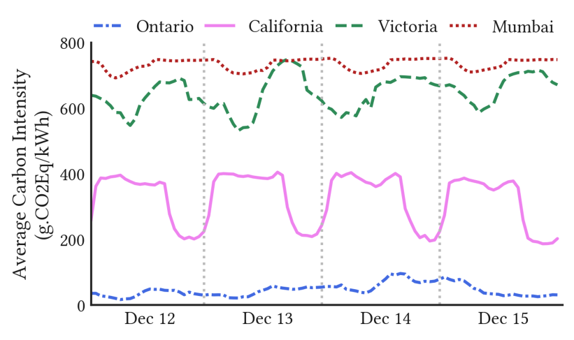
Figure 1. The carbon-intensity of energy supplied by the electric grid can vary by 6-43$\times$ temporally and spatially.

To illustrate, Figure 1 shows that grid energy’s carbon-intensity can vary by 6$\times$ over a day (in California) and by 43$\times$ across regions (between Ontario and Mumbai). The magnitude and variability of grid energy’s carbon intensity depends on the mix of energy sources used to generate it. Traditional fossil fuel-based energy sources tend to exhibit high carbon intensity with negligible variance. In contrast, renewable generation sources, such as from solar and wind, have zero carbon emissions but exhibit highly variable energy output. As a result, the proportion of local renewable versus fossil fuel energy sources, along with the variability in energy’s demand, determines the magnitude and variance of grid energy’s aggregate carbon intensity at a specific location. For instance, since California has a high solar penetration, its energy’s carbon intensity has a low average magnitude but is highly variable. In contrast, since Mumbai generates its energy primarily by burning fossil fuels, its energy’s carbon intensity has a high average magnitude and low variability.

Leveraging spatiotemporal variations in energy’s carbon intensity requires workload flexibility along multiple dimensions. Fortunately, most computing workloads have significant performance, temporal, and spatial flexibility that enables adjusting the intensity, time, and location of their execution to better align with the availability of low-carbon energy. For instance, batch ML training jobs often have temporal flexibility that enables them to be suspended during high-carbon periods and resumed during low-carbon periods (Wiesner et al., 2021). Similarly, an interactive inference request for object detection may have spatial flexibility that enables migrating them to a location with a low carbon intensity. The insights above have led to an implicit assumption within the research community that systems can harness computing workloads’ flexibility to significantly reduce their carbon emissions.

Of course, the benefits of carbon-aware spatiotemporal workload shifting depend on both energy and workload characteristics, i.e., variability in energy’s carbon intensity across different times and regions along with the dimensions and degrees of workload flexibility. If energy’s carbon intensity at some location is relatively stable, such as in Mumbai, then temporal shifting is less effective. In addition, most workloads have limits to their flexibility due to deadline- and latency-based Service Level Objectives (SLOs), privacy regulations, resource constraints, and inaccurate forecasts that prevent fully exploiting variations in carbon. For example, an interactive web request cannot be delayed, and may be subject to regional data privacy regulation, such as GDPR (European Parliament and Council of the European Union, 2016), that restrict spatial migration. Even without privacy restrictions, if there are no nearby locations with low-carbon energy, spatial migration may be infeasible due to additional latency overheads that violate an application’s SLO. Likewise, a batch ML training job may have a completion deadline that prevents delaying it, and requires processing a large dataset that imposes a high overhead for spatial migration. In general, some workloads may not be able to reduce carbon without significantly compromising performance.

Understanding and quantifying the potential for reducing carbon emissions at a global scale via spatiotemporal workload shifting given the constraints above is crucial for informing ongoing research efforts. While there has been preliminary work on quantifying carbon reductions for a small number of geographical regions and batch ML training jobs (Strubell et al., 2020; Dodge et al., 2022; Wiesner et al., 2021), there has not been a comprehensive large-scale analysis that encompasses multiple types of workloads, a wide range of geographical regions across the earth, and various dimensions and degrees of workload flexibility.

To address the problem, we conduct a large-scale longitudinal analysis of historical carbon intensity data worldwide to quantify the upper-bound on the carbon reduction possible through temporal and spatial workload shifting. Our analysis includes traces of hourly average carbon intensity from 123 regions worldwide and covers a three year period from 2020 to 2022. The primary finding from our analysis is that the upper bound on carbon savings from spatiotemporal workload shifting is often modest, and that simple policies can yield most of the benefits. Thus, contrary to conventional wisdom, i) carbon-aware spatial and temporal workload shifting is likely not a panacea for significantly reducing cloud platforms’ carbon emissions, and ii) pursuing further research on sophisticated policies is likely to yield diminishing returns. We highlight many of the insights from our analysis below.

• Currently, more than 70% of regions worldwide have minimal daily variations in carbon intensity due to their reliance on fossil fuel-based or nuclear power generation.

• Nearly all regions exhibit cyclical changes in carbon intensity every 24 hours, influenced mostly by daily demand cycles rather than the presence of solar energy.

• While the long-term trend in worldwide carbon intensity of electricity is downward, global power grids have not experienced an overall shift towards greener energy sources from 2020 to 2022. While some regions have reduced their energy’s carbon intensity, others have increased it.

• For a real-world workload, the average carbon savings from temporal shifting are limited even if the workload has significant performance and temporal flexibility. This occurs because large jobs benefit the least from temporal shifting but typically dominate the resource and energy consumption in real-world workloads.

• Spatial migration offers substantial carbon savings, although they may be constrained by capacity limitations in the greenest regions. The savings may be less in practice due to restrictions on spatial migration due to migration overhead, latency SLOs, and privacy regulations.

• In the current scenario, geographical regions are strictly ranked based on their carbon footprint. Consequently, there is little need for sophisticated region-hopping policies, and migrating to the greenest available region once would yield most of the potential savings.

2. Background

Below, we provide an overview of grid energy’s carbon intensity data, as well as the workload characteristics that affect carbon-aware spatiotemporal workload shifting.

2.1. Grid Carbon Intensity

Our analysis uses historical time-series data for grid energy’s carbon-intensity (in g$\cdot$CO₂eq/kWh) at over 100 locations worldwide. As mentioned in §1, grid energy’s carbon-intensity changes over time based on the mix of generators required to satisfy a variable demand. Of course, the grid’s energy demand varies based on human behavioral patterns, e.g., day/night, weekday/weekend, etc., and weather, which influences the energy necessary for indoor heating and cooling. The electric grid is generally divided into different regions that are operated by their own balancing authority, i.e., Independent System Operators (ISOs) and Regional Transmission Organizations (RTOs), which must satisfy the region’s demand using a variety of generators with different characteristics, such as fuel types, capacities, ramp rates, and, importantly, carbon intensities. The grid’s daily demand is largely met by the day-ahead electricity market, which operates on an hourly basis. Any variations in demand within an hour are handled by the real-time market, which operates on either 5 or 15 minutes intervals. The instantaneous changes in demand or generation occur at the seconds-to-minutes level and are handled by spinning or frequency reserves.

The average carbon intensity of electricity for a specific region at any instant is the average of the carbon intensity for each of its generators weighted by their energy output. Many generation sources have zero carbon intensity, including nuclear, geothermal, hydroelectric, solar, and wind. In addition, solar and wind energy, which are the fastest growing energy sources (Moya, 2022), are “non-dispatchable” generation sources, i.e., their generation is variable. Fossil fuel-based generation such as coal, oil and natural gas, in contrast, have higher emissions, and consequently, a higher carbon intensity. Each region’s mix of generators also differs based on its unique climate and access to natural resources. For example, while some regions have abundant hydro power due to the presence of large rivers, such as in the northwest U.S. , others have abundant solar power, such as in the southwest U.S. In addition, the variability in grid-tied solar and wind’s zero-carbon energy output manifests as variations in grid energy’s carbon intensity. Thus, regions with more solar and wind tend to have more carbon intensity variations.

Until recently, the carbon-intensity of grid energy was opaque to consumers, since generation data was not easily available. However, balancing authorities have begun to publicly release information about the set of active generators and their real-time energy output via web APIs. Carbon information services, such as electricityMap (Maps, 2022) and WattTime (WattTime, 2022), combine this real-time generation information with models based on each generator’s characteristics to infer grid energy’s real-time carbon-intensity in each region, and make it available via web APIs. As discussed in §3, we collect multiple years of this data to use for our analysis.

Note that our analysis focuses narrowly on grid energy’s average carbon-intensity, which falls under Scope 2 emissions in the GHG protocol (Protocol, 2022). The use of grid energy accounts for the vast majority of datacenters’ operational emissions, which include Scopes 1 and 2. Importantly, we do not analyze Scope 3 emissions for either datacenters or the electric grid. Scope 3 mostly covers embodied carbon emissions that result from the production of the products and services a company uses. For example, building a datacenter or power plant also incurs carbon emissions. While Scope 3 emissions are important, they are more difficult to accurately measure and optimizing them, e.g., by increasing server lifetime, selecting “greener” suppliers, etc., generally has a less direct effect on operations. In addition, we also focus our analysis on average carbon emissions, rather than marginal carbon emissions, since the GHG protocol only requires reporting the former. Energy’s marginal carbon-intensity is the carbon-intensity of satisfying the next unit of energy demand. The GHG protocol does not use marginal carbon intensity largely because accurately measuring it is not possible, as it requires knowing when each generator and load starts and stops.

2.2. Workload Spatiotemporal Flexibility

Cloud datacenters serve two broad classes of workloads – batch and interactive – that each have their own dimensions and degrees of spatiotemporal flexibility.

Batch Workloads. Common batch workloads include data processing tasks, machine learning training, scientific computing, and simulations. Such workloads desire high throughput and do not have strict latency needs. Consequently, batch workloads generally include jobs that have some degree of “slack” and thus may be delayed, although not indefinitely. Schedulers often exploit this slack by deferring batch jobs’ start time, i.e., forcing them to wait in a queue, or periodically interrupting their execution. Cluster schedulers, such as Google’s Borg (Burns et al., 2016), Kubernetes (Burns et al., 2016) and Slurm (Jette et al., 2002), generally defer or interrupt batch jobs to satisfy higher-priority requests, either by terminating low priority jobs or checkpointing their state and resuming them later. As we discuss, such schedulers can also defer or interrupt jobs when energy’s carbon-intensity is high to lower carbon emissions. Batch jobs have a wide range of characteristics: from computationally-intensive to data-intensive, from large memory footprints to small memory footprints, and from long running times to short running times. These characteristics, particularly the size of their memory and disk state, affect the overhead of spatially migrating batch jobs as carbon emissions vary across regions. As we discuss, our analysis mostly ignores such overheads to provide an upper bound on carbon reductions from spatially migrating batch jobs. In addition, as mentioned in §1, regulatory policies, such as HIPPA and GDPR, may also prevent spatially shifting batch jobs outside a region, which we consider.

Interactive Workloads. Interactive workloads include small server requests, such as web and inference requests, that require a low latency response. While such requests cannot be delayed and have no temporal flexibility, they can often be flexibly routed to different datacenters for servicing. For example, prior work has proposed policies for migrating (or routing) web requests to datacenters in global Content Distribution Networks (CDNs) based on datacenter load, electricity prices (Qureshi et al., 2009), and energy (Mathew et al., 2012; Gupta et al., 2019). Of course, routing requests based on carbon intensity is also possible. The primary constraint for spatially migrating requests is the additional latency incurred when routing them further from their source. As above, regulatory policies may also prevent spatially migrating interactive workloads.

3. Objectives and Methodology

The primary goal of our analysis is to quantify an upper bound on carbon savings from spatiotemporal workload shifting. Given carbon intensity’s variations and computing’s substantial workload flexibility, our hypothesis was that spatiotemporal workload scheduling could yield significant reductions in computing’s carbon emissions. To quantify carbon savings and evaluate our hypothesis, we focus on answering the specific research questions below. We then outline our methodology for answering these questions.

1. Global Carbon Analysis. What are the characteristics of grid energy’s carbon intensity worldwide? How does its magnitude, variance, and periodicity vary across regions? How has it changed in recent years? (§4).

2. Temporal Workload Shifting. How much carbon savings are possible from temporally shifting delay-tolerant batch workloads? How do the savings vary with workload characteristics, such as job length and slack? (§5).

3. Spatial Workload Migration: How much savings are possible from spatially migrating interactive workloads? How might latency SLOs and regional privacy regulations impact carbon savings? What is the optimal policy for minimizing carbon emissions? (§6).

Importantly, as we discuss in later sections, our real-world trace-driven analysis invalidates our hypothesis above. The primary finding from our analysis is that the upper bound on carbon savings from spatiotemporal workload shifting is modest, and that simple policies can yield most of the benefits. This led to additional questions below on the implications.

1. Implications: What are the implications of this analysis for system operators and the research community? How will the electric grid evolve in the future? How can our analysis guide carbon optimizations in both current and future grids? (§7).

3.1. Analysis Setup

Below, we provide details on our i) carbon intensity data sources, ii) workload characteristics, iii) approach to deriving carbon emissions with and without leveraging workload flexibility, and iv) finally metrics for quantifying average and absolute carbon savings.

3.1.1. Carbon Intensity Data

We collected carbon intensity traces for 123 different grid zones spread across the globe from 2020 to 2022 using the electricityMaps (Maps, 2022) API. Each trace reports energy’s average carbon intensity, measured in grams of carbon dioxide equivalent per kilowatt-hour (g$\cdot$CO₂eq/Wh), every hour. The hourly resolution is the highest resolution for average carbon intensity data that is currently available from public sources. As we show in §4, since grid energy’s carbon intensity rarely varies significantly within 2-3 hour periods, higher resolution data would likely not change the results of our analysis. The 123 locations cover most of the data centers operated by the major cloud providers, including Amazon Web Services, Google Cloud Platform, Microsoft Azure, Alibaba, etc.

Dimension	Range / Description	Source
Type	Interactive, batch, service	(Tirmazi et al., 2020; Cortez et al., 2017)
Length (h)	0.01, 1, 6, 12, 24, 48, 96, 168	(Tirmazi et al., 2020; Cortez et al., 2017)
Deferrability	Fixed or 1-10$\times$	(Ambati et al., 2020; Rodrigo et al., 2018)
Interruptibility	Zero overhead
Resource Usage	Energy-optimized 100% usage	(Tirmazi et al., 2020; Cortez et al., 2017)
Job Arrival Time	Every hour of the year.
Job Origin	$\sim$2700 locations	(Nygren et al., 2010)

Table 1. Workload characteristics, flexibility dimensions and degrees, and configurations.

3.1.2. Workload Configuration

Table 1 outlines the workload configurations used in our analysis. We define workload characteristics across six dimensions as described below.

1. Job Length is the amount of time a job needs to complete its execution without interruption. We examine a range of job lengths that map to interactive jobs (1 minute or less), small batch jobs (1hr to 24hrs), long batch jobs (24-168hrs), and uninterruptible service jobs ($>$168hrs). The range of job lengths and values within that range are based on version 3 of Google’s Borg cluster trace (Tirmazi et al., 2020; Bashir et al., 2021a).

2. Deferrability characterizes the temporal flexibility of a job to delay the start of its execution based on its slack, which dictates the maximum delay possible. Prior work suggests that practical waiting times for batch jobs are generally between a few minutes to less than 24 hours (Ambati et al., 2020; Rodrigo et al., 2018). However, to quantify an upper bound on carbon savings, we vary our slack from 1-10$\times$ a job’s running time, which translates to 1 hour on the lower end and 10 weeks on the higher end for the job lengths we consider.

3. Interruptibility defines the performance flexibility of a job. An interruptible job can be paused and resumed without a significant loss of computation. While suspending and resuming a job incurs some time and energy overhead (based on an application’s memory footprint) that increase emissions, our analysis ignores it, since we focus on quantifying an upper bound on carbon savings.

4. Resource usage captures the aggregate amount of computing resources used over some time period, such as CPU-hours and memory-hours. In our case, we use real-world traces from Azure and Google to find the fraction of total resource usage across all job lengths. We use these fractions to compute the expected carbon savings across all the jobs in these workloads.

   

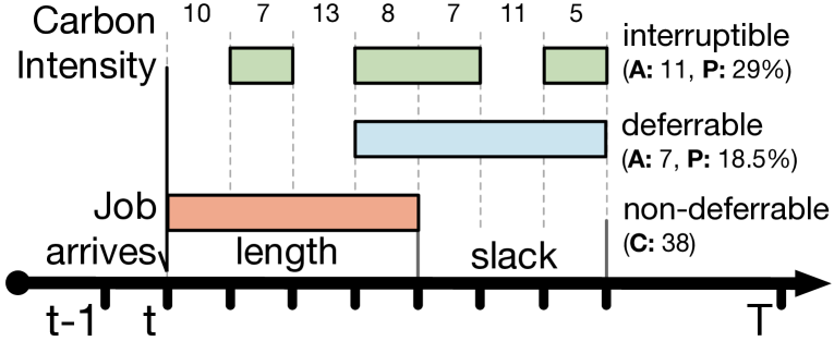
   Figure 2. An illustration of workload shifting based on temporal and performance flexibility showing carbon emissions (C), absolute carbon savings (A), and % carbon savings (P) for deferrable and interruptible jobs.

5. Job arrival time is the submission time of a job. Since jobs can potentially arrive at any point of the day, we consider all the possible job starting times in our carbon traces. As our trace is collected at hourly granularity, jobs can start at the hour boundary and there are 8760 potential start times over a year. We compute carbon savings at all the start time and report the average results along with the standard deviation.

6. Job origin is the geographical location where a job originates. This is an important metric since different locations have different magnitude and variability in their carbon intensity, which dictates the maximum benefits of temporal and spatial workload shifting. For temporal workload shifting, we analyze the carbon savings across all 123 locations. For spatial workload shifting, we estimate the origin of the jobs based on Akamai’s CDN trace (Nygren et al., 2010), where the load at each of the 2700+ locations represents the jobs in a given region. Given this trace, we compute the fraction of jobs that map to, i.e., are closest to, each of the 123 location in the carbon trace, and use the relative weights of locations to compute the aggregate carbon savings for spatial migrations.

3.1.3. Metrics.

We present both the relative carbon savings of spatiotemporal workload shifting for specific locations, as well as the absolute carbon savings. Below, we define both metrics and how we calculate them.

• Relative savings is the percentage difference between carbon emissions after the spatiotemporal workload shifting and a carbon-agnostic baseline where no workload flexibility is present and a job runs as soon as it arrives.

• Absolute savings is the absolute difference between carbon emissions after the spatiotemporal workload shifting and the carbon-agnostic baseline. It is measured in g$\cdot$CO₂eq/kWh and a higher value is better.

• Relative to global average savings is the ratio of absolute carbon savings from workload shifting and the global average carbon intensity of 368.39 g$\cdot$CO₂eq/kWh.

3.2. Analysis Workflow

Below, we describe the high-level workflow for all temporal and spatial workload shifting policies.

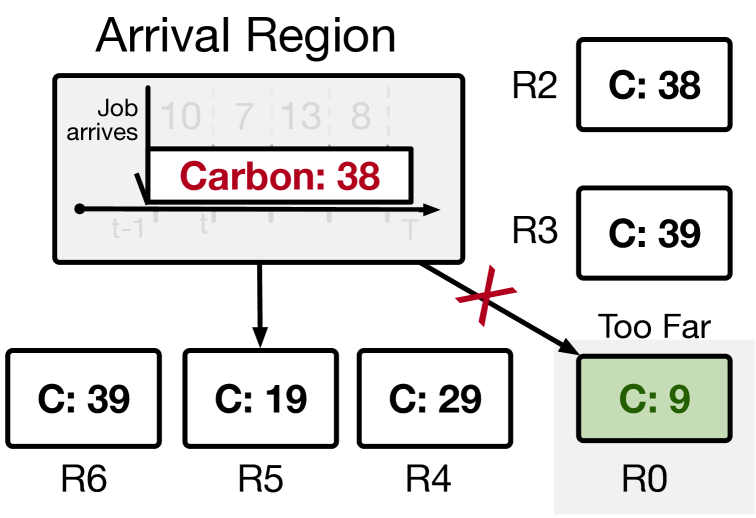
Figure 3. An illustration of workload shifting based on spatial and performance flexibility showing carbon emissions (C) for various regions.

3.2.1. Temporal Workload Shifting.

In our temporal analysis, the different dimensions of a job include its length, ability to defer and related slack, and the ability to interrupt. We assume that we have perfect knowledge of the future carbon intensity and job length. Figure 2 shows our methodology for computing carbon savings under different dimensions. In a non-deferrable or baseline scenario, a job arrives at time $t$ and immediately starts running. In our toy example, such an execution yields 38 units of carbon emissions. If the job is deferrable, we find contiguous slots with minimum cumulative carbon emissions that can fit a given job. Our problem maps well to the standard k-element subarray with minimum sum (Bentley, 1984), where the length of the array is equal to the sum of job length and slack. In our example, the job is deferred to provide 7 units of absolute savings and 18.5% relative savings. Finally, for interruptible jobs, we find k minimum elements in an array, considering no overhead, to find the slots that can finish the job. In the example, the interruptibility leads to absolute savings of 11 units and relative savings of 29%. We repeat this analysis for all the job arrival times and present the mean and standard deviation.

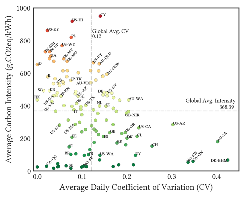
Figure 4. Average carbon intensity and average daily variabilityfor 123 regions around the globe. Labeled points are regions with cloud datacenters and regions with extreme carbon intensities (Hawaii and Cyprus).

3.2.2. Spatial Workload Shifting.

In our spatial analysis, the different dimensions are the job length, the different regions the job can migrate to, and the policy it uses to decide on the migration. As with our temporal analysis, we assume we know the job length and carbon intensity across all the regions in the world. Figure 3 shows how spatial shifting works. A job arrives in a given region and without any spatial migration, its carbon emissions are 38 units. However, during the same time period, the job would have a different amount of carbon emissions if it ran in one of the other regions. Under a “global” setting, the job can migrate to any region in the world, including the R0 region in the figure. However, a job may have a latency target or regulations that prevent it from moving to the greenest region. As a result, it may only be able to migrate to R5, which reduces its savings from spatial shifting. We define various regions in our analysis based on the geographical boundaries. The amount of carbon savings are calculated similar to the temporal analysis.

4. Global Carbon Analysis

Before analyzing the efficacy of temporal and spatial workload shifting for optimizing the carbon emissions of different types of cloud workloads, we begin with an analysis of the carbon intensity of electrical energy across the earth. Our analysis extracts workload-independent observations of the electric grid’s carbon intensity, which will inform our analysis of spatial and temporal workload shifting.

4.1. Carbon’s Magnitude and Variance

Since spatiotemporal workload shifting exploits differences in grid carbon intensity across time and regions, we analyze carbon traces from 123 regions across all give continents to understand their characteristics. Note that many of these regions have cloud data centers from hyperscaler cloud providers. Our analysis examines the average carbon intensity of each region and hourly variations in the carbon intensity, expressed as the coefficient of variation of each region’s carbon intensity. Figure 4 depicts the average and the coefficient of variation (CV) of each region. The dotted lines in the figure represent the average carbon intensity (CI) and the average CV across all regions. As shown, the dotted lines also partition the figure into 4 quadrants, that represent four combinations of low and high CI and low and high CV, e.g., the bottom left quadrant is the low-low quadrant where regions have low CI and low CV and so on.

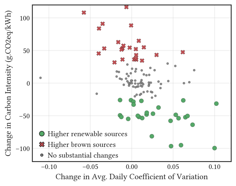
Figure 5. Change in average carbon intensity and daily variability from 2020 to 2022. A negative change indicates the value of the variable decreased over time.

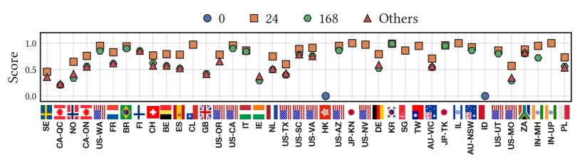
Figure 6. Periodicity scorefor 40 regions with data centers (aws, azure, gcp), the two most common periods are 24 and 168 hour period. The regions are ordered by their average carbon intensity from lowest to highest.

Overall, electric grids that largely depend on fossil fuels to generate electricity have above average (“high”) carbon intensity, while regions with a high degree of renewable sources such as hydro, geothermal, solar, and wind have below average (“low”) carbon intensity. Similarly, since electricity generation from fossil fuels tends to be stable over time, grids that derive electricity from such sources exhibit low variations in carbon intensity. Conversely, grids with higher fractions of intermittent sources, such as wind and solar, exhibit higher variations in hourly carbon intensity.

Figure 4 reveals a number of insights. In particular, the data shows that a significant number (46%) of regions have above-average carbon intensity ($>400$ g$\cdot$CO₂eq/kWh) due to a high reliance on brown sources in many parts of the world. At the same time, many (54%) of the regions also have below average ($<400$ g$\cdot$CO₂eq/kWh) carbon intensity. This implies that workloads from regions that lie in the top two quadrants will benefit from spatial workload shifting by migrating workloads to cloud regions in the bottom two quadrants, and can potentially yield significant emission reductions. For example, there is a 40$\times$ difference in average CI between the highest and lowest regions. The figure also reveals that a majority of regions have below average CV (i.e., lie in the left half), with fewer than 43% of the regions with above average CV. As we will see, the lower the CV, the less effective temporal workload shifting (§5). Many regions with a high carbon intensity also have a low CV due to stable clean generation, e.g., from nuclear, hydro, and geothermal. Even for many regions in the bottom two quadrants (with below-average CI due from using clean energy), relatively few lie in the right half of the figure, with above average CV.

Thus, overall few regions will see significant benefits from temporal shifting methods. Of the regions in the right half, those in the high-high quadrants will see the highest absolute reductions. Overall, the clustering of regions in various quadrants indicates that on a global scale, carbon intensity has a medium average magnitude, but varies widely, with a relatively low average variance.

4.2. Long Term Trends

The carbon intensity of electricity in each region depends on that region’s energy mix and production levels. The mix has changed over time, particularly as various grids attempt to decarbonize and transition to lower carbon sources, e.g., by deploying more solar and wind farms. To understand how grids are evolving in each region, we next analyze the changes in energy’s carbon intensity over a 3 year period. Figure 5 shows the change in each region’s average carbon intensity and CV from 2020 to 2022. Ideally, we would want the change in CI to be negative and the change in CV to be positive, as this would indicate lower emissions due to increased renewable sources.

We derive clusters for Figure 5 using the K-Means++ (Arthur and Vassilvitskii, 2007) heuristic with input $k=3$ for three different groupings with: positive, negative, and no changes in the regions’ mix of energy sources. The figure shows that approximately 23% of regions lowered their carbon intensity, while the CI actually increased in 20% of the regions. Regions are classified with $\pm$0.01 CV changes and $\pm$25 g$\cdot$CO₂eq/kWh as insignificant changes — roughly, 57% of regions fall into this category. Thus, for most regions, there has not been a meaningful change in CI over a 3-year period, indicating that significant changes in grid CI is a slow process and thus the conclusions from our analysis are likely to hold for the next several years. We discuss the implications of long term trends in §7.

4.3. Periodicity Analysis

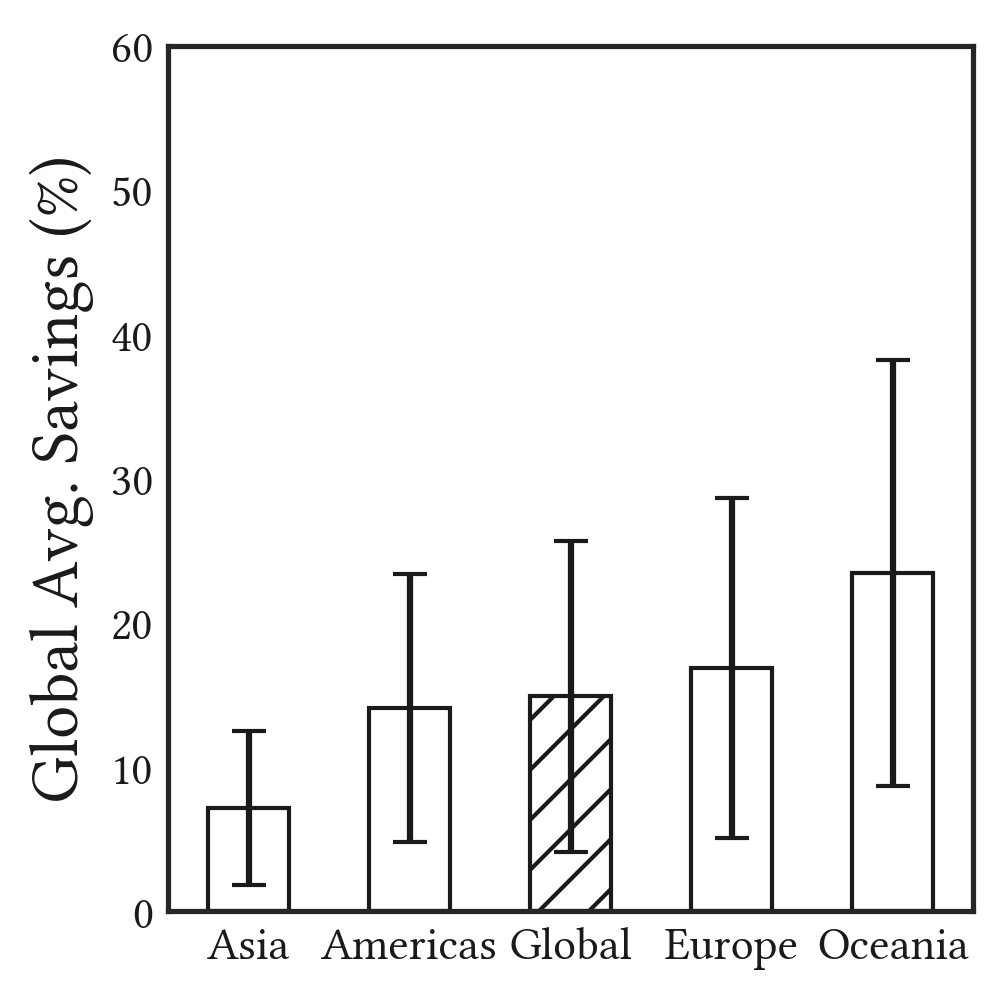
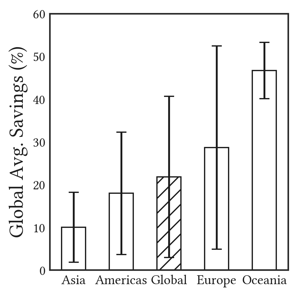
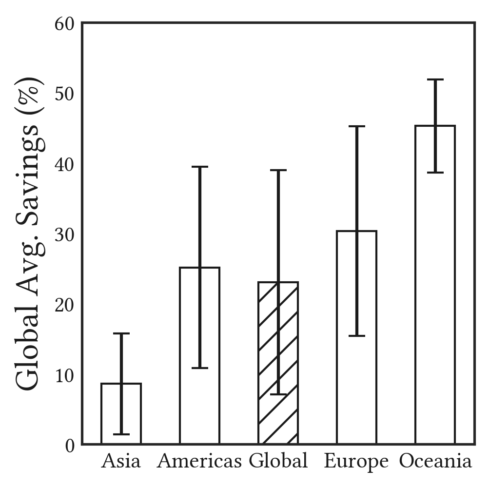
(a) Equal	(b) 80-20 Split	(c) Azure Trace	(c) Google Trace

Figure 7. Estimation of global and regional carbon reductions through temporal shifting of workloads under different mixes of job lengths and datacenters. Slack is 10$\times$. The figure illustrates the relative carbon reduction achieved across different scenarios, showcasing average savings ranging from 14 to 23%.

Apart from their hourly variations, the carbon intensity of a region’s grid also exhibits periodicity at longer time scales. Intuitively, the electricity demand of a grid follows a diurnal pattern across days and nights. Since generation must match demand, the mix of sources used to meet that time varying demand follows similar daily patterns, which in turn influences the resulting carbon intensity. We conducted time series analysis to estimate the degree of periodicity present in the carbon intensity trace of each region. Our analysis yields a periodicity score between 0 and 1, with 0 indicating no period exists and 1 indicating that the time series has exactly the same pattern for that particular period.

Figure 6 depicts the detected period within each trace for 40 geographic regions with hyperscale datacenters, along with their periodicity score. As shown, 35 out of the 40 regions exhibit a 24 hour period in the carbon intensity variation with a periodicity score of 0.5 or higher. Most of these regions also exhibit a weekly period (168 hours period) due to repeating weekday-weekend effects. Only two regions, namely Hong Kong and Indonesia, show a period of zero, indicating a high reliance on fossil fuels, with the mix of generation source and the resulting carbon intensity remaining unchanged overtime. Overall, the presence of daily periods indicates that carbon intensity values exhibit similar diurnal patterns from one day to the next and are predictable. This periodicity and predictability is beneficial for temporal workload shifting methods, which defer work to the future with the expectation of low carbon periods occurring regularly.

5. Temporal Shifting

Below, we quantify the benefits of temporal shifting globally for different workload mixes (§5.1) and different degrees of for deferring (§5.2) and interrupting (§5.3) jobs. We focus solely on batch workloads, since we assume interactive workloads have no temporal flexibility.

5.1. Global Carbon Savings

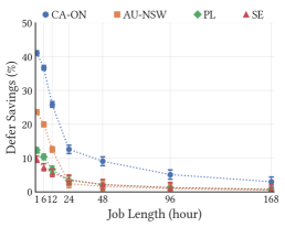
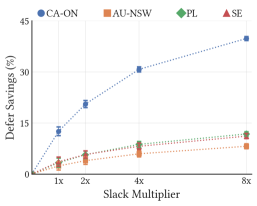
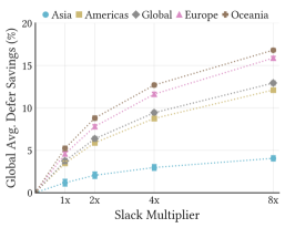
(a) Fixed Slack (24h)	(b) 24h Job Variable Slack (0-8x)	(c) Global Avg. Savings for all job lengths

Figure 8. Comparison of Deferrability Savings across four Regions: Poland, Australia, Ontario, and Sweden. The diverse carbon profiles of these regions result in varied savings. Noticeably, smaller jobs exhibit higher savings as their sizes better align with low carbon periods.

Figure 7 shows the percentage decrease in the workload’s average carbon-intensity relative to the global average carbon-intensity. The global savings ranges from a 14-23% reduction in average carbon-intensity. In the equal weighting and 80/20 split workload mixes, the average savings is $\sim$15%, while for the Azure and Google traces (azu, 2023; goo, 2023), the average savings is $\sim$23%. The Azure and Google traces have a much higher percentage of long jobs ($>$48hrs), which, when combined with the large 10$\times$ slack and interruptibility, increase their flexibility to align with low carbon periods and increase their savings. In particular, in the Google trace, 1% of the very long-running jobs ($>$1 week) account for 90% of resource utilization and energy consumption (Tirmazi et al., 2020). Thus, our analysis assumes that 90% of the energy consumption can be delayed up to 10 weeks, which enables significant flexibility to align with low-carbon periods. The carbon savings also increase as regions have more variations in their carbon intensity, which indicates higher fractions of solar and wind. Since Asia mostly relies on fossil fuels, it has few variations and thus the carbon savings range from only 5-10% across the workload mixes. In contrast, Oceania has a higher percentage of renewables, more variations and more periodicity, which results in carbon savings ranging from 25-50%. Our analysis provides the upper bound on ideal temporal shifting. Actual savings are likely to be much less due to less slack for long jobs, resource constraint that prevents running many jobs during low carbon periods, and uncertain carbon intensity forecasts. We next examine the impact of job length and slack on carbon savings when jobs are deferrable and interruptible.

Key Takeaway. The maximum potential global carbon savings from temporally shifting workloads is around 25%. Regions with more renewables and variation in their energy’ carbon intensity have more potential for savings. Achieving the ideal savings in practice is unlikely, since they largely depend on long jobs having a large slack, no resource constraints, and future knowledge of carbon intensity.

5.2. Effect of Deferrability

Some jobs can be deferred to low-carbon periods, but, once started, cannot be interrupted, e.g., if they cannot be checkpointed. Thus, we analyze the potential for reducing carbon by deferring jobs for a range of different job lengths and slacks. In particular, our analysis specifies slack as both a fixed 24hr value and as a multiple of job length (from 1$\times$-8$\times$). We consider job lengths from 1-168hrs in multiple regions with different characteristics: Poland (PL, with high mean, low CV), Australia (AU-NSW, with high mean, high CV), Ontario (CA-ON, with low mean, high CV) and Sweden (SE, with low mean, low CV).

Figure 8(a) shows the carbon savings from being able to defer batch jobs of varying lengths for a fixed slack of 24hrs. In this case, the carbon savings are relative to a non-deferrable job of the same length running in the same region. The datapoints are averages across all start times over a year. Generally, regions with low coefficients of variation, such as Sweden and Poland, exhibit modest savings of less than 10%, with even lower values observed for longer job durations. This outcome can be attributed to Sweden’s predominantly stable energy mix, primarily composed of hydro and nuclear sources, which results in limited variations that restrict the benefits derived from temporal shifting. In contrast, Ontario and Australia demonstrate more substantial savings of up to 44% and 28% for small 1h jobs, respectively. As job lengths gradually increase, the savings decrease to less than 5% (168-hour jobs) for both regions. However, regardless of the region, larger jobs tend to yield lower savings. This is due to the relatively low fixed slack duration (24h), in comparison to the job lengths. For example, a 168-hour job with a 24-hour slack will have few opportunities to find periods with low carbon intensity compared to smaller jobs.

Next, we analyze how the carbon savings change with increasing slack values, a measure of temporal flexibility of a job. Figure 8(b) plots the carbon savings from deferring a 24hr job as a functional of slack multiplier from 1$\times$ to 8$\times$. Of course, the carbon savings increase as we give the job more slack, since there is more opportunity to align a job’s execution with low carbon periods. Specifically, the savings amount to 12% and 36% with 1$\times$ and 8$\times$ slacks, respectively. Finally, Figure 8(c) shows the average savings globally and across all regions and job lengths. Although Europe and Oceania have higher carbon savings than the global average – up to 15 and 17% respectively – Asia pushes the global average down due to its low renewable penetration. As the slack multiplier increases, the savings increase in higher proportions for regions with higher renewable penetration. Regions like Sweden, Quebec, and Norway have very limited benefits with deferrability because these regions have simultaneously low averages and low coefficient of variations (due to high nuclear and hydro sources), reducing their temporal shifting potential. Overall, deferring jobs yields 12% global carbon savings across all locations and all job lengths with up to 8$\times$ slack, although we note that such high slack values are impractical for long-running jobs, e.g., $>$24hrs.

Key Takeaway. The carbon savings from deferring a job’s start time decrease with job length, with small jobs seeing the greatest benefits. For any given job length, the savings increase with the degree of slack. We find the average carbon savings across all jobs and all regions is less then 12% even for large slack values, with some jobs lengths and some regions seeing up to 45% savings. Our results find that the overall efficacy of temporal shifting will be limited in most regions for most jobs barring the smallest ones.

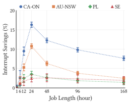
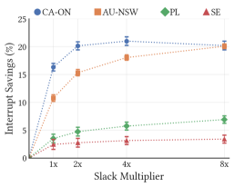
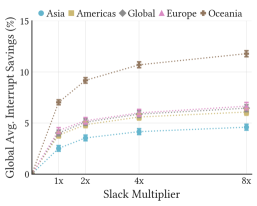
(a) Fixed Slack (24hrs)	(b) 24h Job Variable Slack (1-8x)	(c) Global Avg. Savings for all job lengths

Figure 9. Interruptibility Savings – Peaks at 24h lengths (a), primarily due to deferrability savings. Slack multipliers (b) illustrates the gains for day-long jobs, while (c) showcases the global and continental average savings.

5.3. Effect of Interuptibility

In addition to deferring a job’s start time, the ability to interrupt an already running job when energy’s carbon intensity increases is an additional dimension of flexibility. Interruptibility enables schedulers to pause jobs when energy’s carbon intensity is high and resume them when it is low.

Figures 9(a)-(c) show the additional savings if batch jobs are interruptible in addition to deferrable. Here, we represent the carbon savings as a percentage of additional savings beyond that from deferring jobs (as shown in the previous section). We compare these savings for the same regions and slack settings as discussed in the previous section (§5.2). Figure 9(a) shows the extra average savings for various job lengths (1-168 hours) under the fixed slack case of 24 hours. The carbon savings reaches its peak at 24-hour job lengths — at $\sim$18% — and gradually decreases as the job length increases. The 24-hour jobs exhibit the highest carbon savings because the one-day slack aligns with the job’s length, allowing the interruptibility policy to select very low-intensity periods from two carbon intensity “valleys” within the available 48-hour time window. However, smaller jobs yield lower carbon savings as most of their potential savings are gained simply by deferring them. Likewise, longer jobs exceeding 24 hours follow a similar trend, as the additional savings for these jobs arise from a few lower-intensity carbon hours in the trace.

In addition, Figures 9(b) and (c) show the extra carbon savings from interruptibility as a function of the slack multiplier for 24h jobs and an average across all regions, respectively. Figure 9(b) shows that the carbon savings increases dramatically in Ontario and Australia, particularly with large slack multipliers, reaching up to 20% additional savings. This can be attributed to the relatively higher penetration of renewable energy in these regions, which causes more variations in energy’s carbon-intensity that temporal shifting can exploit. Figure 9(b) also demonstrates that in low variable regions such as Poland and Sweden, the carbon savings plateau quickly at 2$\times$ slack multipliers. This occurs because as the slack increases, the ability to interrupt jobs eventually converges to the same global minima as the deferrable policy, leading to schedules within similar time slots and, consequently, similar emissions. Finally, Figure 9(c) shows the average global and continental interruptible trends. Australia has the highest additional savings of up to 12%, mainly due to its predictable periodicity, allowing the interruptibility policy to consistently use low-intensity time slots throughout the year. In particular, Australia’s average intensity levels can periodically drop by $\sim$$200$ g$\cdot$CO₂eq/kWh, substantially increasing the carbon savings from interrupting jobs. However, the additional carbon savings relative to the global average remains low, reaching only 5% additional savings.

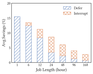
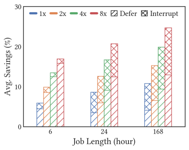
(a) Fixed Slack (24hrs)	(b) Variable Slack (1-8x)

Figure 10. Carbon savings from deferrability and interruptibility for various lengths as a percentage of global average carbon for fixed (24hrs) and variable slack.

Deferrability + Interruptibility Figures 10(a) and (b) show the average carbon savings breakdown for job deferrability and interruptability across all regions. The graphs show the average combined savings from deferrability and interruptability when compared over the same workload mix and slack settings relative to non-deferrable jobs, similar to §5.2 and §5.3. As seen in Figure 10(a) for a 24hr slack, job lengths smaller than 24hr benefit the least from interruptability, with savings reaching only up to 5% for 12hr jobs. As job lengths increase, the effect of interruptability increases, and those from deferrability decrease, although the absolute savings remain small for a fixed slack of 24hrs. Finally, Figure 10(b) shows that similar effects are sustained as the slack multiplier increases. Overall, the carbon savings from interruptability is low for short job lengths – bounded at 5% – and higher for large jobs at 15%. This shows that for large, long-running jobs, the best way to reduce their emissions is through interruptibility.

Key Takeaway. The carbon savings from interrupting a job’s execution increase with job length, with large jobs seeing the greatest benefits. For any given job, the savings increase when slacks are larger than the job lengths. We find the average carbon savings across all jobs and all regions is less than 10% even for large proportional slacks, with some jobs lengths and some regions seeing up to 12% savings. Our results find that the overall efficacy of interruptability depend on the slack being proportional to job lengths.

6. Spatial Shifting

In this section, we quantify the benefits of spatial workload shifting from: (i) migrating to the greenest region in the world (§6.1), (ii) one-to-one migrations between countries with cloud datacenters (§6.2), (iii) using different spatial shifting policies (§6.3), and (iv) migrating interactive workloads (§6.4). Below, we focus solely on carbon savings from spatial shifting; benefits of temporally shifting workloads following the spatial shifting follow from the temporal shifting results for the destination region (see §5). Also, we ignore the overhead of migrating jobs and their data to the destination.

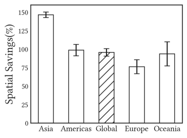
Figure 11. Carbon savings from spatial shifting to the lowest carbon region in the world from various geographical regions.

6.1. Global Carbon Savings

Figure 11 shows the percentage decrease in global carbon, as well as for various geographical regions, relative to the average global carbon intensity. In this case, we assume an always running job that migrates to the region with lowest average carbon intensity for the whole year. In our trace, Sweden has the lowest annual average carbon intensity in the world, $\sim$16g$\cdot$CO₂eq/kWh. As a result, in the extreme case, every job in every other region of the world moves to Sweden and the global average carbon intensity drops by 95.68%. As the average carbon intensity values for various geographical regions are different, depending on their energy mix, the amount of relative savings they get also differ significantly. For example, Europe is the greenest overall region in the world and averaging $\sim$280g$\cdot$CO₂eq/kWh. Thus, its average savings are only 76%, which is significantly less than the global savings. At the other extreme, Asia has the highest average carbon intensity for any geographical region in the world,$\sim$540g$\cdot$CO₂eq/kWh, and thus gets the highest savings from moving to Sweden. Note that the carbon savings from Europe, the least benefiting region, are still massive (more than 4$\times$ compared to the temporal benefits).

Key Takeaway. Spatial shifting to the greenest region in the world yields massive carbon savings when compared to temporal shifting. However, as more regions in the world become greener, the benefits of spatial shifting will start to reduce.

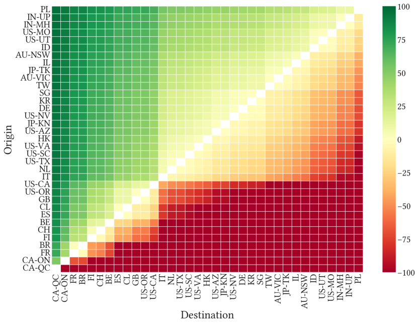
Figure 12. Heat map of carbon savings for spatial shifting from an origin region to a destination region for various GCP datacenters. The darker the green, the higher the savings. For each region on the y-axis, the row shows savings for all possible destinations on x-axis.

6.2. Region-Region Carbon Savings

In presenting the global carbon savings, we implicitly assumed that the lowest carbon region in the world, Sweden, has an infinite capacity and can accommodate jobs from all the other regions in the world. While cloud platforms provide the abstraction of an infinite capacity, it does not hold true in practice. Furthermore, as not all the users leverage cloud resources due to privately-owned datacenters or regulatory considerations, some of the companies may be able to migrate only to specific regions in the world. Below, we relax the assumption of a green region with an infinite capacity and quantify the carbon savings for one-to-one migrations between regions in a smaller subset of the complete trace.

Figure 12 depicts the percentage carbon savings, relative to the originating region, for doing spatial shifting between the origin and destination regions using a heat map. The green boxes represent a decrease in carbon emissions (greener the better) while red boxes represent a reciprocal increase. Also, since we compute the percentage with respect to the region of origin, and not the global average carbon intensity, the amount of savings is always less than 100%. Also, this heat map is symmetrical and we can ignore the red half of the graphs. If we pick a region of origin on y-axis, e.g., Poland (PL), moving along the x-axis gives us the carbon savings for moving to the greenest to the brownest region in the subset, which decrease from 97% for moving to Québec Canada (CA-QC) to 11% for moving to Uttar Pardesh, India (IN-UP). Notably, the savings for Italy (IT) are significant for all the possible destinations. This is due to a large drop in carbon intensity from Italy (375g$\cdot$CO₂eq/kWh) to California, USA (264.232g$\cdot$CO₂eq/kWh), which means that all the regions above Italy can get significant savings from moving their workloads to California, USA. Additionally, if everyone moved to their adjacent region in the carbon ranking, shown by the hypotenuse of the green triangle, the worldwide carbon emissions would decrease by 14%.

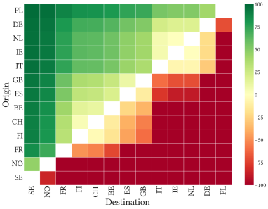
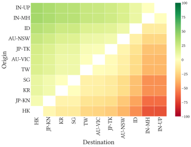
(a) Europe	(b) Asia-Pacific

Figure 13. Carbon savings from spatial workload shifting when restricted to a geographical region (a) Europe and (b) Asia Pacific.

Figure 13 shows a similar heat map, but focuses on the locations in Europe (a) and Asia Pacific (b). The results for Europe are almost similar to the global results as many of the green regions are located in Europe. However, restriction to a region due to GDPR or SLO targets, significantly reduces the extent of carbon savings. For example, if the jobs can only shift to regions within Asia, the maximum achievable savings drop to 40.5% as compared to 96.5% for global scenario.

While we have looked at region-to-region migrations, we have not imposed any capacity constraints. To evaluate the effect of capacity constrains, we compute the capacity fraction in each of the regions by dividing the capacity in each location by the total capacity in the geographical region. The value of capacity for each region is derived from the Akamai CDN trace. After that, we move the load from the brownest location to the greenest location until the destination gets filled. We iterate through the region and stop when each green location is completely full. We compute the savings as the difference between the scenario when no load is migrated versus when it is migrated under capacity constraints. Our results show that, ignoring capacity constraints significantly over-estimates the carbon savings and considering capacity constraints reduce the savings from 98% to 28%.

Key Takeaway. Restrictions on spatial shifting, due to privacy concerns or capacity constraints, significantly reduces carbon savings. Capacity constraints impact carbon savings the most and can reduce savings by more than 70%.

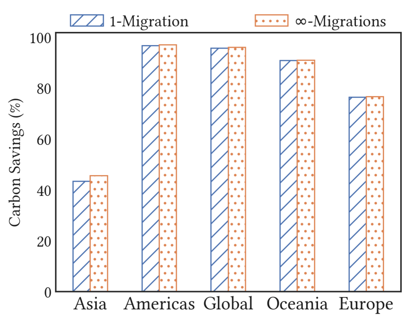
Figure 14. Relative carbon savings from spatially shifting to the greenest region once, 1-migration policy, compared to a greedy carbon chasing policy that migrates infinitely to the lowest carbon region in each time slot in a given geographical region ($\infty$-migration policy.).

6.3. Smart Region-hopping Policies

To this point, our default spatial shifting policy has been to migrate once to the greenest available region. We chose this policy because it enables a simple spatial shifting policy based on historical averages which do not vary significantly on per-year basis. However, as we discussed in §1, there is an assumption that the carbon intensity patterns of various regions vary daily and weekly, and thus may overlap or cross. In this case, a more sophisticated migration policy that hops between locations may yield more carbon savings than a simple one-time migration policy.

To evaluate this hypothesis, we devise another spatial region-hopping policy that is clairvoyant, does not incur energy overhead to migrate, and immediately shifts to the destination. We refer to this policy as $\infty$-migrations, since it can migrate an infinite number of times, as compared to the 1-migration policy we have used so far. Figure 14 shows the amount of relative carbon savings for the $\infty$-migration as well as 1-migration policies. The results show that carbon savings for both policies are quite similar, with $\infty$-migration yielding only slightly higher savings but the difference between them being $<$1%. Thus, migrating once to the greenest region yields the vast majority of the savings and more sophisticated migration approaches that migrate more often are not necessary. Notably, our $\infty$-migration represents a best case policy, as it ignores the overhead of migration. Thus, any practical policy that outperforms 1-migration would have a very tight upper-bound on its savings. In our current electric grid, this upper bound is less than 1%. As a result, there are no practical benefits to sophisticated migration policies.

Key Takeaway. In today’s world, migrating once to the greenest region gives most of the benefits of spatial shifting. Even a clairvoyant policy that ignores the overhead of migration yields at most 2% more carbon savings than 1-migration.

Figure 15. Relative carbon savings, compared to average global carbon intensity, as a function of latency target.

6.4. Effect on Interactive Workloads

Our analysis thus far has focused on long-running batch jobs that may require moving data alongside the job, which incurs overhead and makes the spatial shifting prohibitive. An ideal workload for spatial migration are the interactive requests originating web-based services or inference-serving AI/ML systems. These workloads typically do not have any data dependency and thus their requests can be processed at any location in the world as long as the user receives the response to the request with a certain time frame. If a request can afford additional latency, it can potentially run at a greener datacenter if it can be reached within that time period. As a result, there is a trade-off between the carbon savings and the increase in latency for such interactive workloads.

Figure 15 shows the average carbon savings, compared to average global carbon intensity, as a function of latency SLOs. We use the actual latency data for GCP that provides average latency information between two cloud end points within GCP (for Virtualization at Southern Methodist University, 2023). In each region, as the latency limit increases, the average savings increase, since requests can be routed to greener regions that might be further away. As Figure shows, savings up to 60% can be achieved by a mere 50ms increase in latency. However, the gains are nominal and become flat after 200ms latency. Interestingly, the carbon savings in Asia and Oceania are much less than the other regions initially. This happens because the locations in these regions have similar carbon intensities. As the latency target increases to 300ms, all the regions in the world become accessible, which enables very high carbon savings.

Key Takeaway. Spatially migrating interactive requests yields significant savings ($\sim$60%) for modest increases in latency in regions having locations with different carbon intensity profiles.

7. Conclusions

In this paper, we conducted an empirical analysis of the benefits and limitations of spaiotempoal workload shifting in the cloud. Our results have several important implications.

We show that although there is the potential for some significant carbon savings from spatiotemporal workload shifting, the benefits are often limited in practice. For temporal shifting, these limits derive from a lack of variability in carbon intensity at many locations. In addition, the locations with low variability – where temporal shifting is least effective –tend to be those with the highest absolute carbon emissions – where reducing carbon emissions is most important. Likewise, locations with significant variability tend to have low average carbon emissions, and thus adapting to such variations does not yield significant savings. For spatial shifting, resource constraints will likely limit much of the, potentially significant, carbon savings in practice by preventing most jobs from migrating to the lowest carbon regions. In addition, migration overheads may also prevent many large jobs that consume significant resources and energy, i.e., from processing large datasets, from benefiting from migration.

Of course, as the grid becomes greener our results may change. For example, as more locations adopt renewables, their carbon variability will increase and the global average carbon will decrease. This will increase both the relative and absolute benefit of temporal shifting, since even the highest carbon regions will have variations in their carbon intensity due to renewables. A greener grid will also elevate the importance of more sophisticated spatial shifting policies, as there are likely to be more frequent overlaps in the carbon intensity profiles of different nearby locations. As the grid integrates more intermittent solar and wind to lower its emissions to lower its emissions, it will need more flexible capacity that can dynamically vary its energy consumption to offset variations in these sources. Thus, rather than adapting to how carbon emissions currently vary in the grid, cloud platforms might be more effective in supporting grid’s operations so it can increase the penetration of renewable energy. Our future work will quantify the potential of cloud platforms in supporting such goals.

References

- (1)
- azu (2023) 2023. Azure Public Dataset. https://github.com/Azure/AzurePublicDataset.
- goo (2023) 2023. Google Cluster Data. https://github.com/google/cluster-data.
- Acun et al. (2023) Bilge Acun, Benjamin Lee, Fiodar Kazhamiaka, Kiwan Maeng, Udit Gupta, Manoj Chakkaravarthy, David Brooks, and Carole-Jean Wu. 2023. Carbon Explorer: A Holistic Framework for Designing Carbon Aware Datacenters. In ACM International Conference on Architectural Support for Programming Languages and Operating Systems (ASPLOS). ACM, New York, NY, USA, 118–132.
- Acutt (2018) Nicola Acutt. 2018. Radius: Stories at the Edge, Achieving Carbon Neutrality. https://www.vmware.com/radius/achieving-carbon-neutrality/.
- Ambati et al. (2020) Pradeep Ambati, Noman Bashir, David Irwin, and Prashant Shenoy. 2020. Waiting Game: Optimally Provisioning Fixed Resources for Cloud-enabled Schedulers. In ACM/IEEE International Conference for High Performance Computing, Networking, Storage and Analysis (SC). ACM, New York, NY, USA, 1–14.
- Arthur and Vassilvitskii (2007) David Arthur and Sergei Vassilvitskii. 2007. K-means++ the advantages of careful seeding. In Proceedings of the Annual ACM-SIAM Symposium on Discrete Algorithms. ACM, New York, NY, USA, 1027–1035.
- Bangalore et al. (2023) Srini Bangalore, Arjita Bhan, Andrea Del Miglio, Pankaj Sachdeva, Vijay Sarma, Raman Sharma, and Bhargs Srivathsan. 2023. Investing in the Rising Data Center Economy. https://www.mckinsey.com/industries/technology-media-and-telecommunications/our-insights/investing-in-the-rising-data-center-economy.
- Bashir et al. (2021a) Noman Bashir, Nan Deng, Krzysztof Rzadca, David Irwin, Sree Kodak, and Rohit Jnagal. 2021a. Take it to the Limit: Peak Prediction-driven Resource Overcommitment in Datacenters. In European Conference on Computer Systems (EuroSys). ACM, New York, NY, USA, 556–573.
- Bashir et al. (2021b) Noman Bashir, Tian Guo, Mohammad Hajiesmaili, David Irwin, Prashant Shenoy, Ramesh Sitaraman, Abel Souza, and Adam Wierman. 2021b. Enabling Sustainable Clouds: The Case for Virtualizing the Energy System. In Proceedings of the ACM Symposium on Cloud Computing (SoCC ’21). Association for Computing Machinery, New York, NY, USA, 350–358. https://doi.org/10.1145/3472883.3487009
- Bentley (1984) Jon Bentley. 1984. Programming Pearls: Algorithm Design Techniques. Commun. ACM 27, 9 (1984), 865–873.
- Brown et al. (2020) Tom B. Brown, Benjamin Mann, Nick Ryder, Melanie Subbiah, Jared Kaplan, Prafulla Dhariwal, Arvind Neelakantan, Pranav Shyam, Girish Sastry, Amanda Askell, Sandhini Agarwal, Ariel Herbert-Voss, Gretchen Krueger, Tom Henighan, Rewon Child, Aditya Ramesh, Daniel M. Ziegler, Jeffrey Wu, Clemens Winter, Christopher Hesse, Mark Chen, Eric Sigler, Mateusz Litwin, Scott Gray, Benjamin Chess, Jack Clark, Christopher Berner, Sam McCandlish, Alec Radford, Ilya Sutskever, and Dario Amodei. 2020. Language Models are Few-Shot Learners. Advances in neural information processing systems 33 (2020), 1877–1901.
- Burns et al. (2016) Brendan Burns, Brian Grant, David Oppenheimer, Eric Brewer, and John Wilkes. 2016. Borg, omega, and kubernetes. Queue 14, 1 (2016), 10.
- Cortez et al. (2017) Eli Cortez, Anand Bonde, Alexandre Muzio, Mark Russinovich, Marcus Fontoura, and Ricardo Bianchini. 2017. Resource Central: Understanding and Predicting Workloads for Improved Resource Management in Large Cloud Platforms. In Proceedings of the 26th Symposium on Operating Systems Principles (Shanghai, China) (SOSP ’17). Association for Computing Machinery, New York, NY, USA, 153–167. https://doi.org/10.1145/3132747.3132772
- Dodge et al. (2022) J. Dodge, T. Prewitt, R. des Combes, E. Odmark, R. Schwartz, E. Strubell, A. Luccioni, N. Smith, N. DeCario, and W. Buchanan. 2022. Measuring the Carbon Intensity of AI in Cloud Instances. In FAccT. ACM, New York, NY, USA, 1877–1894.
- Etherington (2020) Darrell Etherington. 2020. TechCrunch, Google Claims Net Zero Carbon Footprint over its Entire Lifetime, Aims to only use Carbon-Free Energy by 2030. https://techcrunch.com/2020/09/14/google-claims-net-zero-carbon-footprint-over-its-entire-lifetime-aims-to-only-use-carbon-free-energy-by-2030/.
- European Parliament and Council of the European Union (2016) European Parliament and Council of the European Union. 2016. Regulation (EU) 2016/679 of the European Parliament and of the Council. https://data.europa.eu/eli/reg/2016/679/oj.
- for Virtualization at Southern Methodist University (2023) AT&T Center for Virtualization at Southern Methodist University. 2023. Google Cloud Inter-Region Latency and Throughput. https://lookerstudio.google.com/u/0/reporting/fc733b10-9744-4a72-a502-92290f608571/page/70YCB.
- Gupta et al. (2021) Udit Gupta, Young Geun Kim, Sylvia Lee, Jordan Tse, Hsien-Hsin S Lee, Gu-Yeon Wei, David Brooks, and Carole-Jean Wu. 2021. Chasing Carbon: The Elusive Environmental Footprint of Computing. In 2021 IEEE International Symposium on High-Performance Computer Architecture (HPCA). IEEE, New York, NY, USA, 854–867.
- Gupta et al. (2019) Vani Gupta, Prashant Shenoy, and Ramesh Sitaraman. 2019. Combining Renewable Solar and Open Air Cooling for Internet-scale Distributed Networks. In e-Energy. ACM, New York, NY, USA, 303–314.
- Hanafy et al. (2023) Walid A. Hanafy, Qianlin Liang, Noman Bashir, David Irwin, and Prashant Shenoy. 2023. CarbonScaler: Leveraging Cloud Workload Elasticity for Optimizing Carbon-Efficiency. arXiv:2302.08681 [cs.DC]
- Jette et al. (2002) Morris A. Jette, Andy B. Yoo, and Mark Grondona. 2002. SLURM: Simple Linux Utility for Resource Management. In In Lecture Notes in Computer Science: Proceedings of Job Scheduling Strategies for Parallel Processing (JSSPP) 2003. Springer Berlin Heidelberg, Berlin, Heidelberg, 44–60.
- Ludvigsen (2022) Kasper Groes Albin Ludvigsen. 2022. The Carbon Footprint of ChatGPT. https://towardsdatascience.com/the-carbon-footprint-of-chatgpt-66932314627d.
- Maps (2022) Electricity Maps. 2022. Electricity Map. https://www.electricitymap.org/map.
- Masanet et al. (2020) Eric Masanet, Arman Shehabi, Nuoa Lei, Sarah Smith, and Jonathan Koomey. 2020. Recalibrating Global Data Center Energy-use Estimates. Science 367, 6481 (2020), 984–986.
- Mathew et al. (2012) Vimal Mathew, Ramesh Sitaraman, and Prashant Shenoy. 2012. Energy-aware Load Balancing in Content Delivery Networks. In INFOCOM. IEEE, Orlando FL, USA, 954–962.
- Microsoft (2022) Microsoft. 2022. Microsoft Ignite, series_periods_detect(). https://learn.microsoft.com/en-us/azure/data-explorer/kusto/query/series-periods-detectfunction.
- Moya (2022) Maria Jimenez Moya. 2022. USAToday, A record 10% of the world’s power was generated by wind, solar methods in 2021. https://www.usatoday.com/story/news/world/2022/03/30/clean-energy-wind-solar-2021/7219298001/.
- Nygren et al. (2010) E. Nygren, R.K. Sitaraman, and J. Sun. 2010. The Akamai Network: A Platform for High-performance Internet Applications. ACM SIGOPS Operating Systems Review 44, 3 (2010), 2–19.
- O’Sullivan (2020) Kevin O’Sullivan. 2020. The Irish Times, Facebook Commits to Net-Zero Carbon Emissions by 2030. https://www.irishtimes.com/news/environment/facebook-commits-to-net-zero-carbon-emissions-by-2030-1.4354701.
- Patterson et al. (2021) David Patterson, Joseph Gonzalez, Quoc Le, Chen Liang, Lluis-Miquel Munguia, Daniel Rothchild, David So, Maud Texier, and Jeff Dean. 2021. Carbon Emissions and Large Neural Network Training. Technical Report. arXiv.
- Pichai (2020) Sundar Pichai. 2020. Google Blog, Our Third Decade of Climate Action: Realizing a Carbon-Free Future. https://blog.google/outreach-initiatives/sustainability/our-third-decade-climate-action-realizing-carbon-free-future.
- Protocol (2022) Greenhouse Gas Protocol. 2022. Greenhouse Gas Protocol. https://ghgprotocol.org/.
- Qureshi et al. (2009) A. Qureshi, R. Weber, H. Balakrishnan, J. Guttag, and B. Maggs. 2009. Cutting the Electric Bill for Internet-Scale Systems. In SIGCOMM. ACM, New York, NY, USA, 123–134.
- Radovanović et al. (2023) Ana Radovanović, Ross Koningstein, Ian Schneider, Bokan Chen, Alexandre Duarte, Binz Roy, Diyue Xiao, Maya Haridasan, Patrick Hung, Nick Care, Saurav Talukdar, Eric Mullen, Kendal Smith, MariEllen Cottman, and Walfredo Cirne. 2023. Carbon-Aware Computing for Datacenters. IEEE Transactions on Power Systems 38, 2 (2023), 1270–1280.
- Rodrigo et al. (2018) Gonzalo P Rodrigo, P-O Östberg, Erik Elmroth, Katie Antypas, Richard Gerber, and Lavanya Ramakrishnan. 2018. Towards Understanding HPC Users and Systems: A NERSC Case Study. J. Parallel and Distrib. Comput. 111 (2018), 206–221.
- Shepardson and Bose (2019) David Shepardson and Nandita Bose. 2019. Reuters, Amazon Vows to be Carbon Neutral by 2040, buying 100,000 Electric Vans. https://www.reuters.com/article/us-amazon-environment/amazon-vows-to-be-carbon-neutral-by-2040-buying-100000-electric-vans-idUSKBN1W41ZV.
- Smith (2020) Brad Smith. 2020. Official Microsoft Blog, Microsoft will be Carbon Negative by 2030. https://blogs.microsoft.com/blog/2020/01/16/microsoft-will-be-carbon-negative-by-2030/.
- Souza et al. (2023) Abel Souza, Noman Bashir, Jorge Murillo, Walid Hanafy, Qianlin Liang, David Irwin, and Prashant Shenoy. 2023. Ecovisor: A Virtual Energy System for Carbon-Efficient Applications. In ACM International Conference on Architectural Support for Programming Languages and Operating Systems (ASPLOS). ACM, New York, NY, USA, 252–265.
- Strubell et al. (2020) Emma Strubell, Ananya Ganesh, and Andrew McCallum. 2020. Energy and Policy Considerations for Modern Deep Learning Research. In AAAI Conference on Artificial Intelligence (AAAI). ACM, New York, NY, USA, 13693–13696.
- Tirmazi et al. (2020) Muhammad Tirmazi, Adam Barker, Nan Deng, Md E Haque, Zhijing Gene Qin, Steven Hand, Mor Harchol-Balter, and John Wilkes. 2020. Borg: The Next Generation. In European Conference on Computer Systems (EuroSys). ACM, New York, NY, USA, 1–14.
- WattTime (2022) WattTime. 2022. WattTime. https://www.watttime.org/.
- Wiesner et al. (2021) Philipp Wiesner, Ilja Behnke, Dominik Scheinert, Kordian Gontarska, and Lauritz Thamsen. 2021. Let’s Wait Awhile: How Temporal Workload Shifting Can Reduce Carbon Emissions in the Cloud. In Proceedings of the 22nd International Middleware Conference (Middleware). ACM, New York, NY, USA, 260–272.