Developments and Further Applications of Ephemeral Data Derived Potentials

Abstract

Machine-learned interatomic potentials are fast becoming an indispensable tool in computational materials science. One approach is the ephemeral data-derived potential (EDDP), which was designed to accelerate atomistic structure prediction. The EDDP is simple and cost-efficient. It relies on training data generated in small unit cells and is fit using a lightweight neural network, leading to smooth interactions which exhibit the robust transferability essential for structure prediction. Here, we present a variety of applications of EDDPs, enabled by recent developments of the open-source EDDP software. New features include interfaces to phonon and molecular dynamics codes, as well as deployment of the ensemble deviation for estimating the confidence in EDDP predictions. Through case studies ranging from elemental carbon and lead to the binary scandium hydride and the ternary zinc cyanide, we demonstrate that EDDPs can be trained to cover wide ranges of pressures and stoichiometries, and used to evaluate phonons, phase diagrams, superionicity, and thermal expansion. These developments complement continued success in accelerated structure prediction.

I Introduction

Machine learning methods have transformed computational materials science Schmidt et al. (2019); Kulik et al. (2022). They have been applied to predict material properties Bhadeshia, MacKay, and Svensson (1995); Sutton et al. (2019); Garrido Torres et al. (2021); Weinreich et al. (2022), develop new density functionals Tozer, Ingamells, and Handy (1996); Snyder et al. (2012); Nagai, Akashi, and Sugino (2020), and train highly accurate interatomic potentials on large quantities of data Behler and Parrinello (2007); Bartók et al. (2010); Deringer, Caro, and Csányi (2019). These machine-learned potentials enable simulations over much larger length- and time-scales than those feasible with ab initio methods such as density functional theory (DFT) Hohenberg and Kohn (1964); Kohn and Sham (1965), at a comparable level of accuracy. Some successful applications of machine learned potentials include crack propagation in silicon Bartók et al. (2018), the high-temperature high-pressure phase diagram of hydrogen Cheng et al. (2020), demonstrating the influence of quantum effects on phases of water and ice  Cheng et al. (2019) and Ge-Te-based phase change materials Sosso et al. (2012); Mocanu et al. (2018), to name a handful of examples among many.

The development of machine-learned potentials is a highly active field and there are already many implementations to choose from. The primary differences between them arise from the choice of atomic descriptors and the fitting method Behler and Parrinello (2007); Bartók et al. (2010); Thompson et al. (2015); Zhang et al. (2018); Pickard (2022); Shapeev (2016); Drautz (2020); Dusson et al. (2022); Batatia et al. (2022); Musaelian et al. (2023); Behler and Csányi (2021); Behler (2021); Chen and Ong (2022); Choudhary et al. (2023). Pioneering developments in machine learning the energy landscapes of extended systems were made by Behler and Parrinello Behler and Parrinello (2007), as well as Csányi and co-workers Bartók et al. (2010). More recently, classes of local potentials that are systematically improvable by increasing the size of the basis, such as the moment tensor potentials (MTP) Shapeev (2016) and the atomic cluster expansion (ACE) Drautz (2020); Dusson et al. (2022), have been developed. Message-passing neural networks take inspiration from chemical intuition Nigam et al. (2022); Batatia et al. (2022). Another promising development is the construction of large-scale graph neural networks covering extensive swathes of the periodic table Chen and Ong (2022); Choudhary et al. (2023).

In addition to research into the development of appropriate atomic descriptors Behler (2011); Bartók, Kondor, and Csányi (2013); Willatt, Musil, and Ceriotti (2019); Musil et al. (2021), substantial effort has been devoted to developing efficient schemes for the training database generation Smith et al. (2018). Traditionally, training data consist of experimental structures, supplemented by manually constructed defect and surface prototypes Deringer, Caro, and Csányi (2019). However, more recent methods have enabled automated construction of datasets without experimental input.

Molecular dynamics (MD) simulations can be used to train the potential on selected uncorrelated snapshots Behler and Parrinello (2007); Novikov et al. (2020); Deringer, Caro, and Csányi (2019); Miksch et al. (2021). This frequently includes an element of active learning Podryabinkin and Shapeev (2017); Zhang et al. (2019), where the potential is updated when it encounters a badly described structure. It is possible to consciously bias the MD runs towards configurations badly described by the potential, requiring fewer steps to obtain sufficient sampling of the energy landscape van der Oord et al. (2023); Kulichenko et al. (2023). Another promising method is to use techniques inspired by structure prediction, in particular random search, to create ab initio datasets Pickard (2022); Dolgirev, Kruglov, and Oganov (2016); Hajinazar, Shao, and Kolmogorov (2017); Hajinazar et al. (2021); Deringer, Pickard, and Csányi (2018); Deringer et al. (2018).

Structure prediction is a prominent component of modern materials science; understanding materials’ structures at the atomic level allows for a quantum mechanical prediction and description of their properties Oganov et al. (2019); Conway, Pickard, and Hermann (2023). Perhaps the most straightforward technique for first-principles structure prediction is Ab Initio Random Structure Searching (AIRSS) Pickard and Needs (2006, 2011), which explores energy landscapes through the relaxation of many randomly generated structures to nearby local minima. Through sufficient samples and aided by constraints ensuring the initial random structures are chemically sensible, low-enthalpy arrangements of the constituent atoms are identified. Other approaches also exist, notably evolutionary Glass, Oganov, and Hansen (2006); Lonie and Zurek (2011) and particle-swarm optimisation Wang et al. (2010), as well as minima/basin hopping Wales and Doye (1997).

The success of ab initio structure prediction over recent decades Pickard and Needs (2007a, 2010); Liu et al. (2020); Pickard and Needs (2006); Duan et al. (2014); Peng et al. (2017); Liu et al. (2017) is largely due to the development of DFT-based methods which can accurately determine candidate structure energies. DFT’s quantum mechanical foundation allows it to replicate the underlying smoothness of the energy landscape, resulting in robust behaviour for all configurations of atoms. This is essential for structure prediction. However, the need in DFT to account for the electronic structure incurs a significant computational cost. This cost can scale cubically with the number of atoms, while the size of the configuration space to be searched ultimately increases exponentially Pickard and Needs (2011).

Machine learned potentials can ameliorate the cubic scaling problem Hajinazar, Shao, and Kolmogorov (2017); Deringer et al. (2018); Ouyang, Xie, and Jiang (2015); Deringer, Csányi, and Proserpio (2017); Patra et al. (2017); Tong et al. (2018); Podryabinkin et al. (2019); Gubaev et al. (2019); Thorn et al. (2019); Bisbo and Hammer (2020); Kaappa, del Río, and Jacobsen (2021) and a class of neural-network potentials, Ephemeral Data-Derived Potentials (EDDPs) Pickard (2022), were recently developed specifically for high-throughput structure prediction. To date, the approach has been validated with two published searches. Its first application was the prediction of a new high pressure phase of silane (SiH₄). Silane was one of the first systems to be studied with AIRSSPickard and Needs (2006), but the recent work using EDDPs has uncovered a previously unseen structure which contains twelve formula units (f.u.) in the primitive cell and becomes thermodynamically stable around $300$ GPa Pickard (2022). Recently, EDDPs were employed in the study of a ternary hydride system. Following the recent experimental claim of room temperature superconductivity at close-to-ambient pressures in the Lu-H-N system Dasenbrock-Gammon et al. (2023), ternary hydride systems have been the focus of several computational studies Xie et al. (2023); Huo et al. (2023); Hilleke et al. (2023); Ferreira et al. (2023). Of these studies, the only one to identify a thermodynamically stable ternary structure at ambient pressure leveraged EDDPs for the structure search, exploring more of the composition space and searching with larger unit cells Ferreira et al. (2023); Kim et al. (2023).

The training scheme for the EDDPs is inspired by the AIRSS approach and closely integrated with the AIRSS software package. In AIRSS, sensible structures are generated by placing atoms randomly into a unit cell and then adjusting their positions to satisfy a set of chemically inspired constraints. The structures are then relaxed to their nearest local minima. Normally, this is done using the CASTEP DFT package Clark et al. (2005), but with the EDDPs, repose (see Sec. IV.2) fulfils this role. Through sufficient samples, low-enthalpy arrangements of the constituent atoms are identified.

This work is organised as follows. In Sec. II, we summarise the main features of the EDDPs, notably their tightly-constrained, physically inspired descriptors. In Sec. III, we explain our training scheme, which is based on a wide exploration of chemical space in small cells and uses a light-weight neural network of typically just five nodes in a single hidden layer. In Sec. IV, we explain the software implementation of EDDPs, how they can be used to carry out simulations, and suggest some best practices for generating a high-quality potential. In Sec. V, we highlight several key features of the EDDPs through a series of case studies. The EDDPs are smooth and exhibit size transferability (for instance, a Pb potential trained on no more than six atoms can be used to successfully run MD simulations with thousands of atoms). EDDPs can be used to study a wide range of stoichiometries and pressures and can describe complex systems such as metal-organic frameworks (MOFs). The EDDPs, originally designed to accelerate structure search, can be used to calculate phonon dispersions, run MD, and accurately predict phase diagrams.

II Main Features of the EDDPs

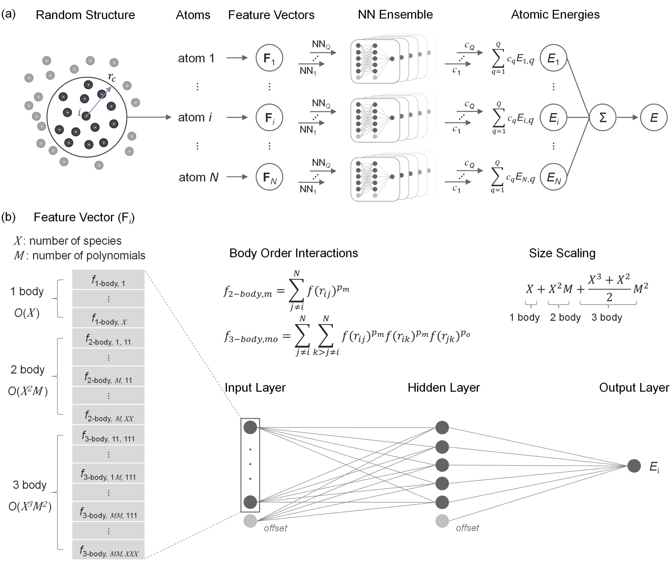
Figure 1: (a) Key stages of generating a potential: building feature vectors from atomic environments, training of multiple individual potentials to generate an ensemble before obtaining a single potential from a weighted fit across this ensemble (Q is total size of ensemble, with each individual potential indexed by q). (b) Feature vectors are constructed by concatenating the basis functions for each species and each body-order interaction. The total size of this vector depends on the number of functions (M), the number of body-order interactions included in the potential and the number of species (X). These feature vectors are passed through a shallow neural network to yield an atomic energy. The atomic energies for all atoms are summed up to give the total energy.

In this section we outline briefly the EDDP method; a more complete description is available in Ref. (22). Like many interatomic potentials, EDDPs approximate the total potential energy by a sum of atomic contributions ¹⁰:

$$E_{\mathrm{tot}}=\sum_{i}E_{i}=\sum_{i}E(\mathbf{F}_{i}),$$ (1)

where $\mathbf{F}_{i}$ is a feature vector encoding a local atomic environment and i runs over all atoms in the system. In principle, the function $E(\mathbf{F}_{i})$ may be determined in numerous ways, including linear, Gaussian process, or neural network regression. In the Subsection II.1, we introduce the EDDP feature vector in a linear setting, after which we summarise the neural networks employed in practice (shown in Fig. 1(a)).

II.1 EDDP Feature Vectors

The EDDP feature vector is rooted in the body-order expansions utilised by many classical interatomic potentials. Such expansions express the atomic energies in Eq. 1 in terms of interactions with neighbouring atoms:

$$E_{i}=E^{(1)}_{i}+E^{(2)}_{i}+E^{(3)}_{i}+...$$ (2)

with each term corresponding to an increasing body-order interaction ($E^{(1)}$ is one-body, etc.). Taking inspiration from the physically motivated Lennard-Jones ^{79; 80} and extended Lennard-Jones ⁸¹ potentials, these interactions can be modelled with a linear combination of functions composed of a radial function f(r) raised to a power $p_{m}$. Wang et al. ⁸² have previously proposed using radial functions that are naturally cut-off beyond a radius $r_{c}$. We use a function that follows this approach with the form:

$$f(r)=\begin{cases}2(1-r/r_{c})&r\leq r_{c}\\ 0&r>r_{c}.\end{cases}$$ (3)

The two-body interaction expressed as a sum of these functions is:

$$E^{(2)}_{i}=\sum^{N}_{j\neq i}\sum^{M}_{m}w^{(2)}_{m}f(r_{ij})^{p_{m}}=\mathbf{w}^{T}_{(2)}\mathbf{F}_{i}^{(2)},$$ (4)

where the first summation is over the neighbours j of the central atom i, with distance $r_{ij}$ between them. The second summation is over the total number of functions M with corresponding weights $w^{(2)}_{m}$. The analogous expression to Eq. 4 for the three-body interactions is:

$$E^{(3)}_{i}=\sum^{N}_{j\neq i}\sum^{N}_{k>j\neq i}\sum^{M}_{m}\sum^{M}_{o}w^{(3)}_{mo}f(r_{ij})^{p_{m}}f(r_{ik})^{p_{m}}f(r_{jk})^{q_{o}}=\mathbf{w}^{T}_{(3)}\mathbf{F}_{i}^{(3)}.$$ (5)

The first two summations now run over neighbouring atoms, with the index k corresponding to a third atom that contributes to the interaction. The summations in $m$ and $o$ run over functions with corresponding weights $w_{mo}$. The powers $p_{m}$ are distributed geometrically between a minimum and maximum exponent. By default, the minimum exponent is $2$, ensuring continuity of energies and forces at the cutoff radius ²².

The right-hand sides of Eq. 4 and Eq. 5 show how the two- and three-body interactions can be expressed as a scalar product between a number of weights $\mathbf{w}^{T}$ and a vector $\mathbf{F_{i}}$. When the $\{\mathbf{F}_{i}^{(j)}\}$ for all body-order interactions are concatenated they constitute the feature vector (shown in figure 1 (b)), which defines the local environment of atom $i$:

$$\mathbf{F}_{i}=\mathbf{F}^{(1)}_{i}\oplus\mathbf{F}^{(2)}_{i}\oplus\mathbf{F}^{(3)}_{i}.$$ (6)

The weights ($\mathbf{w}^{T}$) could be found from a linear fit. In practice these linear weights are not used in the EDDP scheme, rather a small neural network is employed with the feature vectors $\mathbf{F_{i}}$ as input.

In the case of multiple species and truncation at three-body terms, this concatenation gives a feature vector of length $X+X^{2}M+\frac{X^{3}+X^{2}}{2}M^{2}$, where $X$ is the number of species and M the number of polynomials. This scaling results from species-centred representations of each body order and the feature vectors are sparse in the case of many species. While the EDDPs include interactions up to three-body by default, two-body potentials can be sufficiently accurate to accelerate structure prediction in non-covalently bonded systems and considerably faster.

II.2 Neural Network

After constructing the feature vectors, a fit is carried out using a neural network with a single hidden layer typically containing no more than $5$ nodes. This small and light-weight neural network makes the cost of fitting the potential negligible compared to the cost of the first-principles calculations. An EDDP can be trained on a small number of central processing units (CPUs), such as might be contained in a laptop.

Since training neural networks involves non-convex optimisation with a stochastic initialisation, two subsequent fits on the same data will typically produce two different potentials. In the EDDP framework, this is exploited to construct an ensemble of several potentials to obtain a composite EDDP. By regularising the fit, ensembles are expected to outperform individual potentials ^{83; 84}.

III How to Train Your EDDP

Several recent studies have demonstrated the success of small-cell training schemes ^{47; 48; 22; 85; 86}. These methods cover a large region of chemical space by using a training set containing many small cells with a wide variety of structures. The computational cost associated with evaluating the DFT energies of datapoints in this way is low compared to methods which rely on MD trajectories of larger systems.

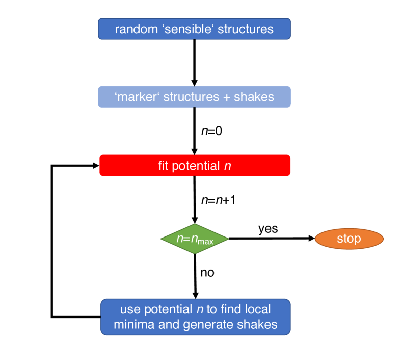
Figure 2: The iterative scheme used to generate a dataset of small-cell structures and train an EDDP on it. Blue rectangles indicate DFT singlepoint energy calculations, with light blue indicating the optional marker structure step. The red rectangle indicates the process of fitting the potential.

The scheme for training EDDPs uses a small-cell method designed to exploit random structure searching to provide diverse, and challenging, datasets. Figure 2 summarises the iterative training. The training dataset is initially comprised of randomly generated structures. It is possible to specify a variety of constraints on how these structures are generated, such as minimum interatomic distances and a number of applied symmetry operations. The exact choices will depend on the task at hand, but the general principle is that this set of structures should be diverse, and include high-energy configurations in order to help the EDDP learn what is not a good arrangement of atoms. The energies for these structures are found with single-point calculations at the DFT level. The number of atoms in these initial structures is typically in the range of $2$-$20$. In the examples in Sec. V, the lowest number of atoms is $2$ for elemental lead, and the highest is $24$ for scandium hydride.

It is possible, but not necessary, to add ‘marker’ structures to the set. These will usually be structures the system is known to adopt, and manually including them helps ensure they are well-described. These structures are ‘shaken’ (subjected to small random distortions). The DFT energies of the new set are calculated and added to the dataset. A first EDDP is trained on the random (and possible marker) structures and then refined in an iterative process. In each iteration the current EDDP is used to relax a set of newly generated random structures to their local minima. The structures corresponding to those minima are also shaken. The energies of these shaken structures and those at the minima are calculated using DFT and added to the dataset. A new EDDP is then trained for the next iteration. The training is terminated after a few, typically five, iterations. The default values for these parameters, along with all others important for the generation of EDDPs, are summarised in table 1.

The cost function used to train the potential takes the form

$$C=\frac{1}{S}\sum_{s}\left|E_{s}-\sum^{N_{s}}_{i}E(\mathbf{F}_{s,i})\right|^{p},$$ (7)

where the index s runs over the total S structures in the training dataset, $E(\mathbf{F}_{s,i})$ is the EDDP energy of atom i, $E_{s}$ is the total DFT energy and $N_{s}$ is number of atoms in each structure. The exponent $p=1.25$, in a compromise between minimising the mean average and root mean square errors. Note that, in contrast to other schemes, forces are not included in the cost function. The low computational cost of energy calculations for small-cells allows for a denser sampling of the energy landscape and the quality of forces from the resulting potentials has proven to be sufficient for many applications (see sec. V for examples of dynamical calculations). In particular, the shaken structures ensure sensible forces by providing information about the potential energy surface near the minima.

On every iteration, the data is split into training, validation, and testing sets at a ratio of approximately 80:10:10. The cost function is minimised using the Levenberg-Marquardt optimisation algorithm ^{87; 88} only on the training set. The validation set is used to implement early stopping ⁸⁹ in order to avoid over-fitting. Finally, the remaining error against DFT is calculated on the testing set in order to assess the quality of the potential.

As discussed in Sec II and shown in figure 1a, an ensemble of potentials is used in the EDDP scheme. The weighted average potential is generated via non-negative least squares (NNLS) ⁹⁰ reusing and fitting to the validation dataset. This combines a small subset of all generated potentials with positive weights; most potentials will have weights of exactly 0, avoiding over-fitting problems arising from an unconstrained least-squares fit ²². The NNLS combines only those potentials important and useful for describing the energy landscape well. This reduces the number of neural network predictions which must be carried out. Combining a number of potentials allows the size of the individual neural networks to be kept small. In our experience, the ensemble usually results in a smaller testing error than any individual potential.

The existence of many individual potentials allows for statistical analysis of the performance of the potential ⁸³. The (unweighted) standard deviation of the predicted energies across the subset of potentials selected by the NNLS is referred to as the ‘ensemble deviation’. Although not a direct measurement of the error with respect to DFT, it provides a useful indicator of how well-constrained the potential is in a given region of structure space. This can be used to bias the structures included in the dataset towards those which are not yet well-described, introducing an additional element of active learning. It can also be used to assess the transferability of potentials. It should be kept in mind that, in principle, it is possible for the deviation to be small even though the error compared to DFT is large⁹¹, however we are yet to observe such a case for any EDDP ensemble. Finally, we use the ensemble deviation to remove pathological structures from high-throughput searches. These pathological structures appear in regions where the potential is not well-constrained and are usually characterised by unreasonably small atomic separations. Such structures will have ensemble deviations of hundreds of eV per atom. This is orders of magnitude larger than well-described structures, whose deviations are of the order of a few meV per atom.

Table 1: Default values of the main parameters governing EDDP training.

Parameter	Default
Radial cutoff, $r_{c}$	$3.75$ Å
Size of hidden layer	$5$
Number of training cycles, n${}_{\text{max}}$	$5$
Number of polynomials, $M$	$5$
Lowest exponent	$2$
Highest exponent	$10$
Number of initial random structures	$1000$
Number of minima per cycle	$100$
Number of shakes per minimum	$10$
Shake amplitude	$0.02$ Å

IV Implementation and Practical Use

As originally implemented, the EDDP package is a set of bash scripts and Fortran codes. These are available under the GPL2 license ⁹², along with AIRSS ⁹³, which the EDDP package uses to generate the training set. The CASTEP DFT package ⁷⁸, with which the EDDP framework has been integrated, is available at no cost under academic license ⁹⁴.

IV.1 Generating EDDPs

The chain script is distributed with the EDDP package and steps through the iterative training scheme discussed in Sec. III. It is executed on a head node and launches jobs on a set of specified compute nodes it must be able to reach via ssh. This is a convenient setup for small- to mid-size personal clusters not inhibited by wallclock time restrictions.

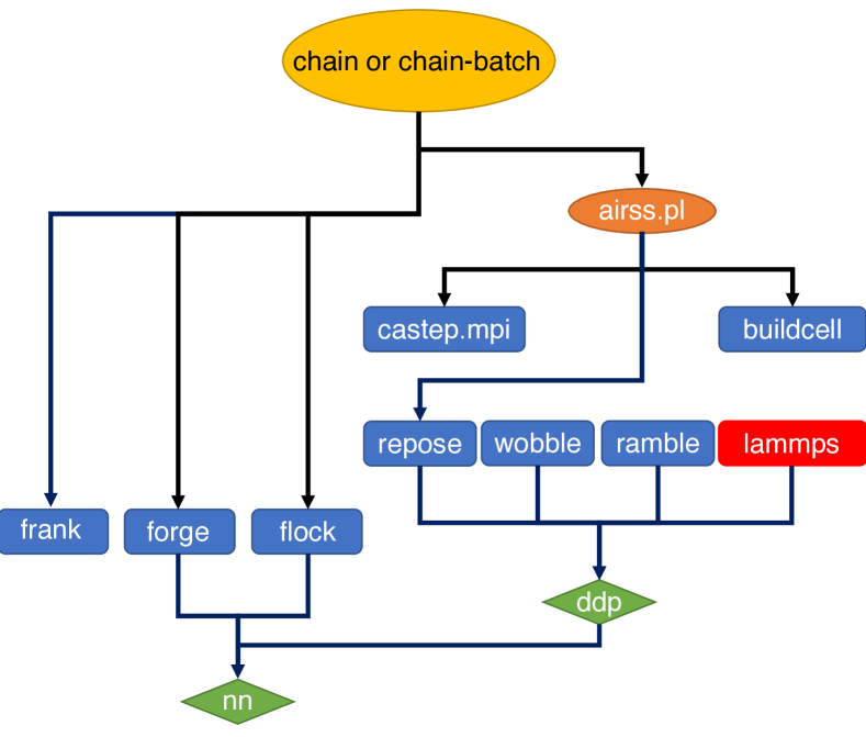
Figure 3: The relationship between the different codes comprising the EDDP framework. Downward arrows indicate a call. Yellow (orange) ellipses represent bash (perl) scripts, blue (red) rectangles represent compiled Fortran (C++) programs, and green rhombi are Fortran modules. For details on the different codes, see the main text.

Figure 3 shows the relationship between chain and the other codes in the EDDP framework. It calls AIRSS, which generates random structures using buildcell, and then calculates their energies using DFT. These calculations are small and run independently, resulting in efficient parallelism and scalability. frank, forge, and flock are responsible for feature vector generation, neural network fit, and NNLS combination of the final potential respectively. flock and forge interface with the neural network via the nn module. repose is the supported geometry optimisation code; it is run through the AIRSS script to generate relaxed structures for the training dataset. All the codes described above are developed in-house and do not use any pre-existing neural-network libraries for Fortran. They currently make use of OpenMP parallelisation and Basic Linear Algebra Subprograms (BLAS) libraries, but detailed profiling and optimisation is yet to be implemented.

From a functionality perspective, the EDDP package provides a self-contained pipeline for data-set generation, potential training, geometry optimisation and dynamical simulations, via the buildcell, repose, ramble and wobble codes. The most unique feature of the EDDP package compared to other Fortran neural network potential implementations is the in-built integration with AIRSS for generation of the data-set of small random structures.

A Julia implementation (developed by one of us) is also available (EDDP.jl) ⁹⁵. This implementation has comparable performance to the Fortran version and allows easy integration with a range of optimisation algorithms, machine learning frameworks, and neural network implementations. It also interfaces with python, allowing packages such as the Atomic Simulation Environment (ASE) ⁹⁶ and phonopy ⁹⁷ to use the EDDPs.

High-performance computing (HPC) clusters with queueing systems are supported using the ddp-batch package, available separately on GitHub ⁹⁸. chain-batch is based on chain, and takes the same command line arguments, but instead of launching the various steps in the training process directly using ssh, it submits them as job scripts to the HPC queueing system. Users are able to specify the scheduler options separately for each of these jobs in a .schedopt file, allowing for the available compute resources and architectures to be employed optimally. chain-batch monitors the status of the HPC jobs and only progresses once the required number of calculations has been completed. If the job is interrupted by wallclock time limitations before then, it is automatically resubmitted. chain-batch is transferable to different HPC systems; so far, it has successfully been used on the SGE-based Thomas cluster hosted at University College London, as well as the Slurm-based Cambridge Service for Data-Driven Discovery (CSD3) and the UK National Supercomputing Service ARCHER2.

IV.2 Running Calculations with EDDPs

Table 2: Summary of simulation codes in the EDDP package.

Programme	Task
repose	Local geometry optimisation
wobble	Finite-difference phonon calculations
ramble & LAMMPS	Molecular dynamics

Table 2 summarises the different codes which use the EDDPs to carry out different types of atomistic calculations. The EDDPs’ original purpose, structure prediction, is enabled by repose, which performs local structural optimisation of atomic configurations and is interfaced with the AIRSS package. In addition, the EDDP suite of codes supports phonon calculations based on the finite differences method ⁹⁹ through wobble, which calculates the vibrational energy, as well as phonon dispersions and densities of states. MD simulations are performed using ramble, as well as through a LAMMPS ¹⁰⁰ interface. These codes interact with the neural network via the ddp module, see figure 3.

Table 3: Single-core performance of potentials used in this work.

System	CPU Time [$\mu$s/atom/step]
Carbon (Fig. 4(b) in section V.1)	475
Lead (section V.2)	324
ScH12 (section V.3)	23781
lcs-Zn(CN)2 (section V.4)	250

repose, wobble, and ramble are Fortran codes, supplied by the EDDP package. They are not fully-featured packages, but rather designed to be workhorses which carry out basic tasks and can easily be integrated into more complex workflows. The EDDP-enabled version of LAMMPS permits a wider range of dynamical simulations to be conducted. The EDDPs are implemented through a new ‘pair-style’ and currently permit OpenMP parallelisation over a single node. Melting point calculations for lead (see Sec. V.2.4) have been computed separately and validated between LAMMPS and ramble.

Both wobble and ramble can automatically construct nearly cubic supercells with a specified number of atoms given any primitive, or base, unit cell. While methods exist to generate such supercells (see e.g. Erhart et al.¹⁰¹), the approach outlined below is more robust to varying orientations of the basis vectors, and therefore more suitable to high-throughput calculations.

A structure with a primitive unit cell basis, $\mathbf{S_{p}}$, can be transformed to a supercell basis, $\mathbf{S_{s}}$, by matrix multiplication,

$$\mathbf{S_{s}}=\mathbf{P}\mathbf{S_{p}},$$ (8)

where $\mathbf{P}$ is an integer matrix. The aim is to choose $\mathbf{P}$ which generates the ‘most cubic’ $\mathbf{S_{s}}$ for a given $\mathbf{S_{p}}$. In our approach, we define a ‘cost function’, $\Delta$, which is agnostic to the unit cell orientation and contains the lattice parameters, $x_{i}$, angles, $\alpha_{i}$, and the target number of unit cells, $N_{\textnormal{target}}$,

$$\Delta=\frac{\sqrt{\sum_{i}\left(x_{i}-\sum_{j}\frac{x_{j}}{3}\right)^{2}}}{\sum_{i}\frac{x_{i}}{3}}\\ -\sqrt{\sum_{i}\cos^{2}\alpha_{i}}+\frac{|N_{\textnormal{target}}-\det{(\mathbf{P})}|}{N_{\textnormal{target}}}.$$ (9)

This cost function is minimised stochastically by applying random changes of $+1$, $0$, or $-1$ to the elements of $\mathbf{P}$. If this change lowers the cost function, then the new $\mathbf{P}$ is accepted. This procedure is continued until a stable $\mathbf{P}$ is found which will contain close to the target number of atoms and have a close-to-cubic lattice shape.

The method described here is distinct from the method of Erhart et al.¹⁰¹, which instead attempts to minimise the off-diagonal terms of $\mathbf{S_{s}}$ and so is sensitive to the specific orientation of $\mathbf{S_{p}}$. Our method is well suited to high-throughput calculations which may encounter non-standard unit cell orientations.

Table 4: Some of the most important parameters for obtaining high-quality EDDPs, along with commonly suitable values and strategies for setting them appropriately for particular cases.

Parameter	Common values	How to determine it	Comments
Radial cutoff $r_{c}$	$\sim 2\times$bond length	Simple hyperparameter search	It is essential to use a sufficiently large $r_{c}$.
			For $r_{c}>5$ Å, it may be beneficial
			to increase the number of polynomials slightly.
Size of input dataset	1000 random & 5500 (shaken)	MAE${}_{\text{testing}}$ >> MAE${}_{\text{training}}$	For systems with multiple elements,
	local minima structures	indicates that more data is necessary	a larger dataset will usually be required.
	(for single-element systems)
Number of polynomials $M$	$5$-$7$	Simple hyperparameter search
Range of minimum	Should encapsulate the	Known experimental structures or	It is important that this is in the right
atomic separations &	range exhibited by the	simple AIRSS-CASTEP search	range; the exact details are not crucial.
volumes per atom	local minima structures

IV.3 Benchmarks

Table 3 summarises the computational performance of the different potentials used in this work. The timing tests have been carried out on a single core of an Apple M1 Pro chip. The systems for which the timings were measured were chosen to reflect the practical applications in section V. All benchmarks are 100-step MD simulations. The Pb benchmark is a solid-liquid coexistence simulation at $0$ GPa; the ScH₁₂ benchmark was carried out at 300 GPa; and the lcs-Zn(CN)₂ benchmark is a MOF at 0 GPa. The different densities explain the large spread of timings. The open structure of the Zn(CN)₂ MOF system gives it the lowest number density of all the systems studied. It therefore yields the fastest benchmark, in spite of the large feature vectors needed to describe the three elements. Conversely, ScH₁₂ at $300$ GPa is significantly denser than all other systems, leading to a larger computational overhead for calculation of the feature vectors.

For carbon, a cubic cell with 800 atoms at a density of 2 g/cm³ was constructed in order to enable comparison with the potentials benchmarked by Qamar et al. ¹⁰². We note that the timings presented in table 3 represent a snapshot of the current performance of the EDDP code suite. Further optimisations, particularly of the feature calculation and GPU porting, are in progress. Nevertheless, the benchmarks demonstrate that the EDDPs are capable of achieving costs competitive with ACE, and an order of magnitude lower than the established methods tested by Qamar et al. ¹⁰². The benchmark suite is available ¹⁰³.

IV.4 Best Practices

The ‘recipe’ for generating an EDDP is straightforward, and the key input parameters have reasonable defaults. For some systems or applications, other values may give better results. In particular, we note that the default radial cutoff, $3.75$ Å, is chosen to obtain fast potentials most suitable for structure search. If a more accurate and transferable potential is required, a higher cutoff must typically be chosen. This is the case for all examples presented in section V.

Table 4 summarises (in roughly descending order of impact) some common strategies for obtaining well-behaved and transferable EDDPs. This is not intended to be an exhaustive list; the case studies described in section V present a wide range of different strategies for generating high-quality EDDPs. However, the parameters summarised in table 4 will provide suitable starting points, especially for those still learning to use EDDPs. All EDDP training parameters can be optimised using hyperparameter searches. This does not require regeneration of the dataset and is hence computationally cheap, especially considering the lightweight nature of the neural network architecture.

V Case Studies

Table 5: The input parameters chosen for the EDDP training as well as the underlying DFT calculations in the different case studies.

	System
Parameter	Carbon	Lead	Scandium hydride	Zinc cyanide
DFT Parameters
Energy cutoff [eV]	600	600	600	600
$\mathbf{k}$-point spacing [$\times 2\pi$ Å-1]	0.05	0.017	0.03	0.04
XC functional	PBE 104 + TS dispersion correction 105	PBEsol 106	PBE	PBE + TS dispersion correction
Structure Building Parameters
Minimum interatomic distance [Å]	$1$-$2$	$2$-$4$	Sc-Sc: $1.79$-$2.79$	$0.4$-$4$
			H-H: $0.60$-$1.46$
			H-Sc: $1.20$-$2.32$
Volume per atom [Å3]	$4$-$11$	$25$-$35$	Sc: $6.9$-$16.1$	$25$-$100$
			H: $1.2$-$4.3$
EDDP Training Parameters
$r_{c}$ [Å]	$5.5$	$7$	$6$	$6$
Number of exponents	$5$	$6$	$5$	$5$
Highest body order	$3$	$3$	$3$	$3$
Number of nodes in hidden layer	$5$	$5$	$5$	$5$
Number of random structures	$1000$	$1000$	$10000$	20000
Number of cycles	5	5	5	5
Number of local minima per cycle	$100$	$100$	$100$	110
Number of shakes per local minimum	$10$	$10$	$10$	10
Total number of structures	$6500$	$6500$	$15500$	32100
Pressure range [GPa]	$0$	$0$-$50$	$50$-$400$	$0$-$10$
Number of EDDPs generated	$250$	$280$	$256$	$405$
Number of EDDPs selected by NNLS	19	14	19	45
MAE [meV/atom]	$64.88$	$3.14$	$25.33$	$44.34$

In this section, we present a series of case studies highlighting different features and capabilities of the EDDPs. Carbon, with its diverse range of allotropes and chemical bonds, is an interesting and difficult test case for machine-learned potentials. Our EDDPs generate smooth potential energy surfaces in good agreement with DFT for a wide variety of different structures. Lead, as a heavy metal, is expensive to describe in DFT, due to the need for both a dense $\mathbf{k}$-point grid and the inclusion of spin-orbit coupling (SOC). Experimentally lead is well-understood, making it a suitable test case. Training an EDDP on high-quality first-principles data enables structure searching and the successful reproduction of its known phase diagram up to $20$ GPa.

Two further case studies, the scandium hydride system under pressure and a MOF, Zn(CN)₂, demonstrate that EDDPs are able to describe systems with more than a single element. For scandium hydride, a single potential can be used to robustly search a range of stoichiometries, across a pressure range of $50-400$ GPa. MD simulations reveal a prediction of superionicity at 350 GPa and 600 K in this system. In Zn(CN)₂, we compute a negative thermal expansion in good agreement with the experimentally observed value, without prior knowledge of the stable structures. These two case studies also reveal good practices for training an EDDP for variable stoichiometry.

All first-principles calculations presented in this work were carried out using the CASTEP plane-wave DFT package ⁷⁸. The EDDP package interfaces with the plane-wave DFT calculations via the AIRSS package, and only requires single-point energies. It can be straightforwardly adapted to different DFT codes, or different total energy methods altogether. The data that supports these case studies is available on MaterialsCloud ¹⁰⁷.

V.1 Smoothness and Transferability: Carbon

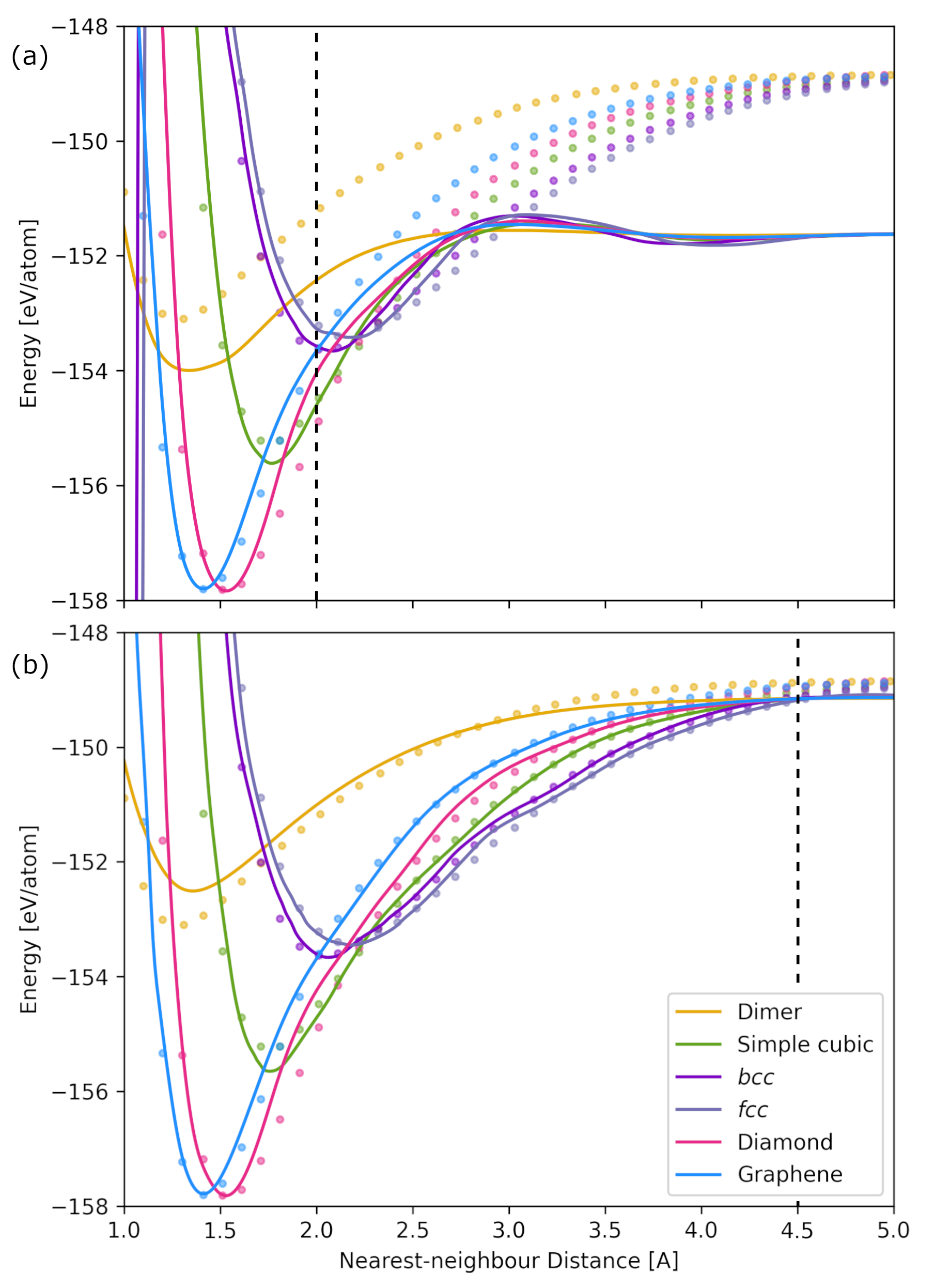
Figure 4: Potential energy curves of a number of carbon structures as a function of distance for (a) an EDDP trained on data with only short minimum atomic separations and (b) an EDDP with longer-range data added. Lines represent EDDP curves and dots represent DFT calculations. Dashed vertical lines indicate the largest nearest-neighbour distance in the respective training sets.

In the context of structure prediction, a machine-learned potential should be smooth, transferable, and robust. A smooth potential is well suited to global optimisation, allowing physically sensible energy minima to be accessed from less physical initial conditions. The potential must also be transferable to describe these diverse initial conditions with sufficient accuracy.

Carbon is the essential element of organic life ¹⁰⁸ and a building block in many diverse and complex molecules. The allotropes of pure carbon are also of continued scientific interest ^{109; 110} and machine-learned potentials have been applied to accelerate their prediction and characterisation ¹¹¹. A difficult and illuminating test is to generate a potential for carbon which is both smooth and transferable to systems far away from idealised diamond- or graphite-like structures. While several transferable Carbon potentials have been developed, they vary significantly in smoothness, as discussed by Qamar et al. in the comparison to their smooth ACE potential ¹⁰², and therefore suitability for structure search.

To highlight the comparative smoothness and transferability of a well-trained EDDP, we train and compare two separate potentials for carbon. The training set for the first potential contains only structures with minimum nearest-neighbour atomic separations between $1$ and $2$ Å. The second potential is trained on a set which contains a larger range of nearest-neighbour distances.

Table 5 summarises the parameters governing the generation of the first potential. $1000$ random structures were used in the training set with minimum interatomic distances of $1$-$2$ Å. $5500$ local minima and shakes were added to the set in $5$ cycles of iterative training. 250 EDDPs were generated from this training data. The NNLS reduced this to 19 for the final potential, which had a testing mean average error (MAE) of $64.88$ meV/atom. This comparatively large error (the largest of all systems in this section) results from the diversity of carbon systems. In many EDDP training sets, a large segment of the error arises from badly described high-energy structures. In this case, however, the test set error when considering only structures within $1$ eV/atom of the ground state is still $63.55$ meV/atom.

The second potential was trained using the same parameters, but $500$ randomly generated structures with minimum C-C separations between $1.75$ and $4.5$ Å and volumes per atom from $40$-$70$ Å were added to the dataset generated above. $100$ identical copies of the isolated carbon atom were also included. This structure is added multiple times to ensure a suitable weighting in the fitting process. We emphasise that other than this, the dataset remained completely random. For instance, the isolated carbon dimer is not included in the training set. 250 EDDPs were again generated from this training data, of which the NNLS selected 14 for the final potential. The testing mean average error was slightly higher at $73.25$ meV/atom in this case. The testing error over structures no more than $1$ eV/atom from the ground state is reduced slightly, to $71.35$ meV/atom.

The potential energy curve for the EDDP trained on smaller interatomic distances is shown in Fig. 4(a). With exception of the dimer, the potential accurately describes all structures around their respective minima, including the simple cubic crystal – an uncommon structure for carbon at low pressure. Any unphysical oscillations in the curves are minor, and their smoothness for atypical structures is enhanced dramatically compared to the potentials tested by Qamar et al.¹⁰² - with the exception of ACE. This is true even in regions with nearest-neighbour distances larger than $2$ Å, yielding a ‘sensible’ if not quantitatively correct extrapolation into this region. A shallow false minimum exists between $3.5$ and $4$ Å, but this can be avoided in structure searches applying chemically sensible constraints.

Fig. 4(b) shows that by augmenting the dataset, the correct description of longer-range interactions can be achieved. The curve now accurately predicts energies at long range, making the potential more suitable for applications such as surface or defect structure searches. No false minima exist in this EDDP.

From this example, we see that that EDDPs are, by construction, smooth. We also show that it is trivial to produce an EDDP which is suitable for the most important regions of structure space - around the minima of the potential energy curves - and straightforward to improve the description of longer-range interactions.

In order to enable comparisons with other carbon potentials in the literature^{102; 112}, we calculated the lattice constant and bulk modulus of diamond, using both the EDDP used to generate Fig. 4(b), and a new EDDP trained (with the same hyperparameters) on the dataset curated by Qamar et al.¹⁰². For the sake of brevity, these two potentials are referred to as EDDPs I and II respectively.

Table 6: The properties of Carbon calculated by a variety of different machine-learned potentials. Values in brackets are the corresponding DFT values.

Potential	Lattice Parameter [Å]	Bulk modulus [GPa]
EDDP I	3.502 (3.572)	580 (431)
EDDP II	3.570 (3.572)	433 (431)
ACE102	N.A.	429 (435)
PANNA112	3.576 (3.584)	431 (425)

Table 6 summarises the properties predicted by these EDDPs, as well as those predicted by ACE¹⁰² and PANNA^{113; 112}, and compares them to the corresponding DFT values. EDDP I disagrees most strongly with DFT. The dataset used to generate EDDP I is much smaller than those used for the ACE and the PANNA potentials, and the EDDP is trained only on the energies. It is designed for transferability and cost-effectiveness to accelerate searches and is not in any way refined to predict properties for diamond. EDDP II, however, predicts properties in excellent agreement with DFT. This demonstrates that the EDDP formalism can produce significantly more accurate potentials when necessary.

Overall, this brief comparison highlights the flexibility of the EDDPs, which can produce both cheap and transferable potentials for searching, as well as accurate potentials competitive with state-of-the-art methods. The balance between the two extremes can be tuned to fulfil the specific task at hand by adapting the training set and hyperparameters.

V.2 (Heavy) Elements: Lead

Lead (Pb), with atomic number 82, is relatively common in nature. It is the the heaviest element with stable isotopes and the end-product of the three most common radioactive decay chains ¹¹⁴. Its ground state structures have been studied extensively up to hundreds of GPa. At ambient temperature, the sequence is fcc $\rightarrow$ hcp $\rightarrow$ bcc with increasing pressure ¹¹⁵. The melt curve has also been investigated both experimentally ^{116; 117; 118} and with DFT ¹¹⁹.

Spin-orbit coupling, a relativistic effect, is an important contribution to the behaviour of heavy elements, as it is proportional to the nuclear charge ¹²⁰. In Pb, it shifts the phase boundaries, renormalises the phonons, and increases the superconducting transition temperature ^{121; 122; 123}. However, the additional computational expense associated with SOC ¹²⁴ prohibits high-throughput DFT searches and ab initio MD. This difficulty is compounded by the need for dense $\mathbf{k}$-point grids to obtain converged DFT energies in metals.

Accelerating such calculations is therefore an important application of machine-learned potentials, enabling structure prediction for previously inaccessible regions of the periodic table. Here, we train an EDDP for Pb, with SOC included in the training dataset, and deploy it for structure searching, phonon calculations, and MD simulations. The resulting pressure-temperature phase diagram up to $20$ GPa and $2500$ K shows good agreement with available experimental data. Compared to DFT, the reductions in computational cost amount to 4-5 orders of magnitude for the structure searches and 7 orders of magnitude for the lattice dynamics.

V.2.1 Training

Table 5 summarises the training parameters used to generate the Pb potential. A norm-conserving pseudopotential (NCP) with two projectors on both the $6$s and $5$d states, and one on the $6$p state, was constructed. The CASTEP pseudopotential string is 3|2.4|12|14|26|60NN:61N:52NN(qc=7). The potential’s error over the whole testing set is $3.14$ meV/atom. When considering only the low-energy structures at most 1 eV/atom from the ground state, this is further reduced by more than half to $1.31$ meV/atom. A separate potential was trained on DFT energies not including SOC. In this case, the default C19 ultrasoft pseudopotential was used but all other parameters were left unchanged. All calculations presented below include SOC unless otherwise stated.

V.2.2 Benchmark Search and Enthalpy Curves

Table 7 compares the number of $8$-atom Pb structures found with DFT and the EDDP per hour. The EDDP is very nearly $5$ orders of magnitude faster than DFT, and easily finds the favourable fcc and hcp structures. Even accounting for the computational expense of generating the DFT training data — which uses only single-point energy calculations — the total computational cost of a thorough structure search is significantly lower with the EDDP. This underlines starkly the challenge of carrying out ab initio structure prediction for heavy metals at the level of accuracy required.

Table 7: The number of $8$-atom structures found per hour per core in the SOC energy landscape of lead using both DFT and the EDDP on $112$ CPU cores.

Method	Number of structures per hour per core
DFT	$0.0004$
EDDP	$37.107$

Next, we use DFT and the EDDPs to calculate the static-lattice enthalpies of the three lowest-pressure known ground states of lead, fcc, hcp, and bcc, up to $75$ GPa. The results are shown in Fig. 5, relative to the hcp enthalpy. The EDDP shows good agreement with DFT for all structures’ enthalpies up to $\sim 50$ GPa and correctly predicts the fcc $\rightarrow$ hcp transition pressure. Fig. 5 also shows the ensemble deviation of the energy estimations as a shaded region around each curve. Beyond $\sim 50$ GPa (the upper limit of the training data), the DFT and EDDP energies begin to diverge, just as the deviations increase. This indicates that ensemble deviations are good predictors of the model’s uncertainty.

The errors in the EDDP predictions are slightly higher at pressures near the edge of the training data ($1.5$-$2$ meV below $\sim 5$ GPa and above $\sim 45$ GPa, versus $1$ meV in the range of $5$-$45$ GPa). This results from the training set being better constrained in the intermediate region of the training pressure range and suggests that training should include a wider range of pressures than those to be studied. In addition, the bcc structure of Pb is less well-described below $15$ GPa, since it is unstable in this regime. Hence it is not found in the training set at the corresponding volumes. The ensemble deviations faithfully reflect these features.

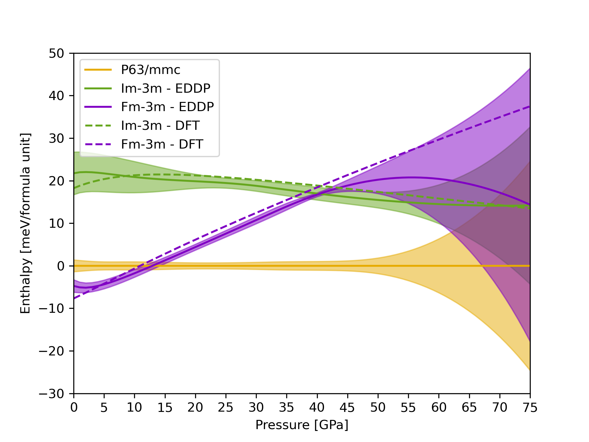
Figure 5: Enthalpies and deviations up to $75$ GPa of the fcc and bcc structures of lead, relative to the hcp enthalpy. The shaded regions indicate the EDDP ensemble deviations.

V.2.3 Lattice Dynamics

In this section we compare phonon calculations of the ground state (fcc) lead structure between DFT and the EDDP at $0$ GPa. The DFT calculations use the finite-difference Caesar code, which accelerates phonon calculations by constructing a number of small non-diagonal supercells ¹²⁵. An $8\times 8\times 8$ $\mathbf{q}$-point grid is found necessary to obtain a phonon dispersion in qualitative agreement with experiment.

Phonon calculations using DFT are very sensitive to small changes in the calculated electronic structure. To obtain well converged calculations, we required higher precision parameters. A plane-wave cutoff of $1000$ eV, $\mathbf{k}$-point spacing of $0.01\times 2\pi$ Å^-1 and an self-consistent field tolerance of $10^{-8}$ eV/atom were used. Furthermore, we increased the ‘standard’ and ‘fine’ Fourier transform grids to include plane waves up to $2\times G_{\text{max}}$ and $2.5\times G_{\text{max}}$, where $G_{\text{max}}$ is the diameter of the reciprocal space cut off sphere.

Fig. 6(a) compares the phonon dispersions calculated using the EDDP with those from DFT and experiment. The theoretical dispersions are calculated both with and without SOC. In both cases the EDDPs reproduce the main features of the phonon dispersion, with particularly good agreement at low frequencies. We find poorer agreement between the EDDP and DFT results when SOC is not included in the calculations.

The EDDP fails to capture the Kohn anomaly at the X point, both with and without SOC. Kohn anomalies are uncommon, and result from a rapid change of the screening of certain lattice vibrations by the electrons ¹²⁶. Kohn anomalies occur along wavevectors which connect different momenta on the Fermi surface, the so-called nesting vectors. It is perhaps not surprising that a machine-learned potential, which integrates out the details of the electronic structure, struggles to capture such a subtle effect of the electron-phonon coupling. Kohn anomalies are strongly localised in reciprocal space; in real space they only occur for very specific extended configurations. It appears that the EDDP simply averages over this anomalous point in the electronic structure. This is not a fundamental limitation of machine-learned potentials. Recently, Wang et al. presented an MTP which successfully reproduced the Kohn anomaly in $\alpha$-Uranium ¹²⁷. This potential was trained on data collected from MD runs of a supercell of $\alpha$-Uranium at a range of pressures and temperatures.

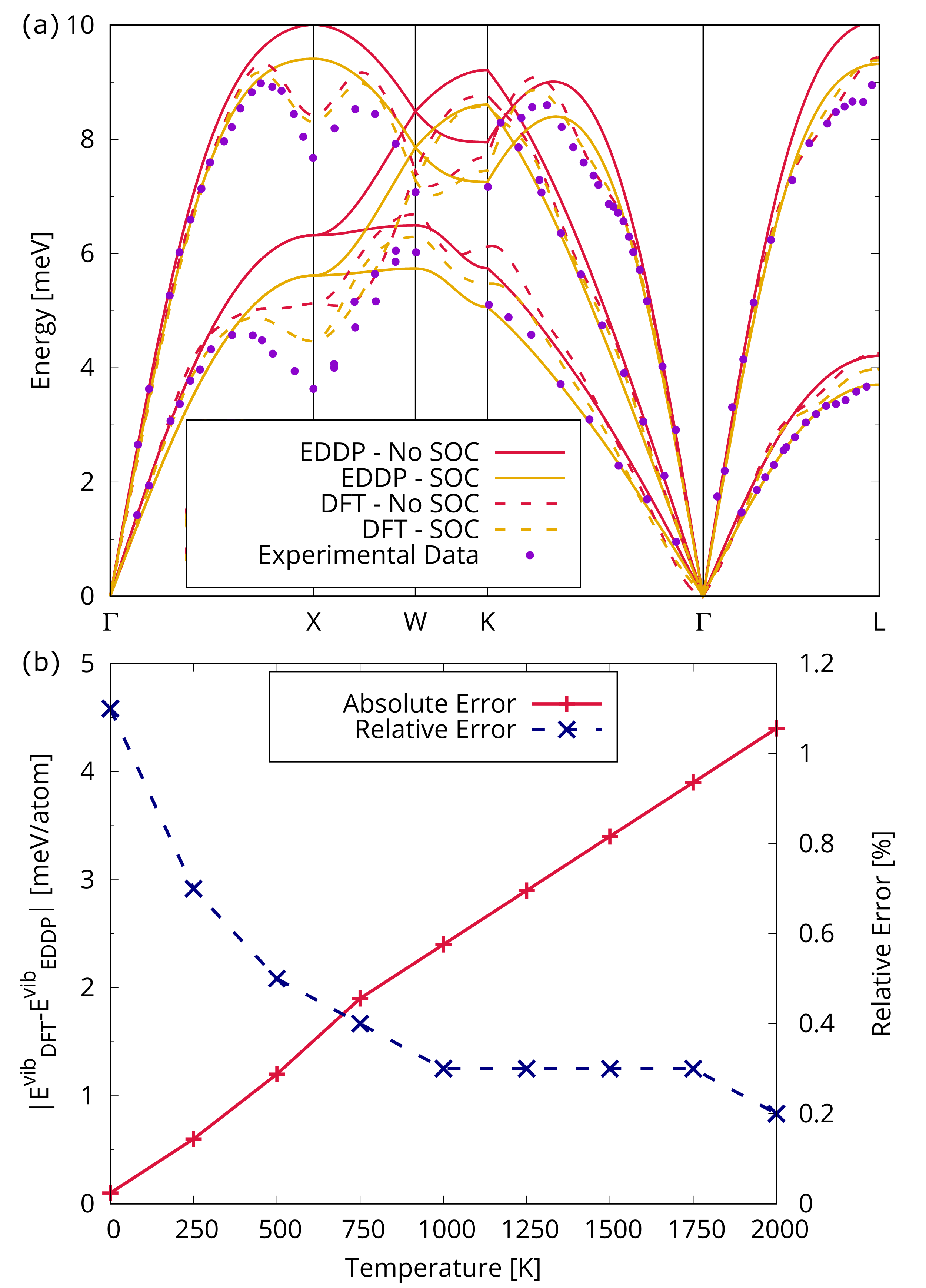
Figure 6: (a) The phonon dispersion of fcc lead, calculated without and with SOC using DFT as well as the EDDP, and compared to experimental data from Brockhouse et al.¹²⁸. (b) The error in the EDDP prediction of the vibrational energy compared to DFT as a function of temperature.

While the EDDP does not capture all the details of the phonon dispersion, it produces good agreement for the total vibrational energy (evaluated by integrating over all phonon modes). This is essential for accurate thermodynamic calculations. Fig. 6(b) summarises the error in the vibrational energies predicted by the EDDP compared to those from DFT, including SOC. The EDDP results are within $5$ meV/atom of the DFT prediction for all temperatures considered. The zero-point energies agree almost exactly, with an error of $0.1$ meV/atom. At $2000$ K, the EDDP phonon energy is $4.4$ meV/atom lower than that from DFT. The relative error decreases with temperature and is less than $1$% from $250$ K. This is remarkable precision for a potential trained only on the energies, at a fraction of the computational cost of the DFT calculations. For these phonon calculations, $42882$ core hours were required for DFT compared to only $0.01$ with the EDDP, a speed-up of more than $6$ orders of magnitude.

V.2.4 Phase Diagram up to 20 GPa and 2500 K

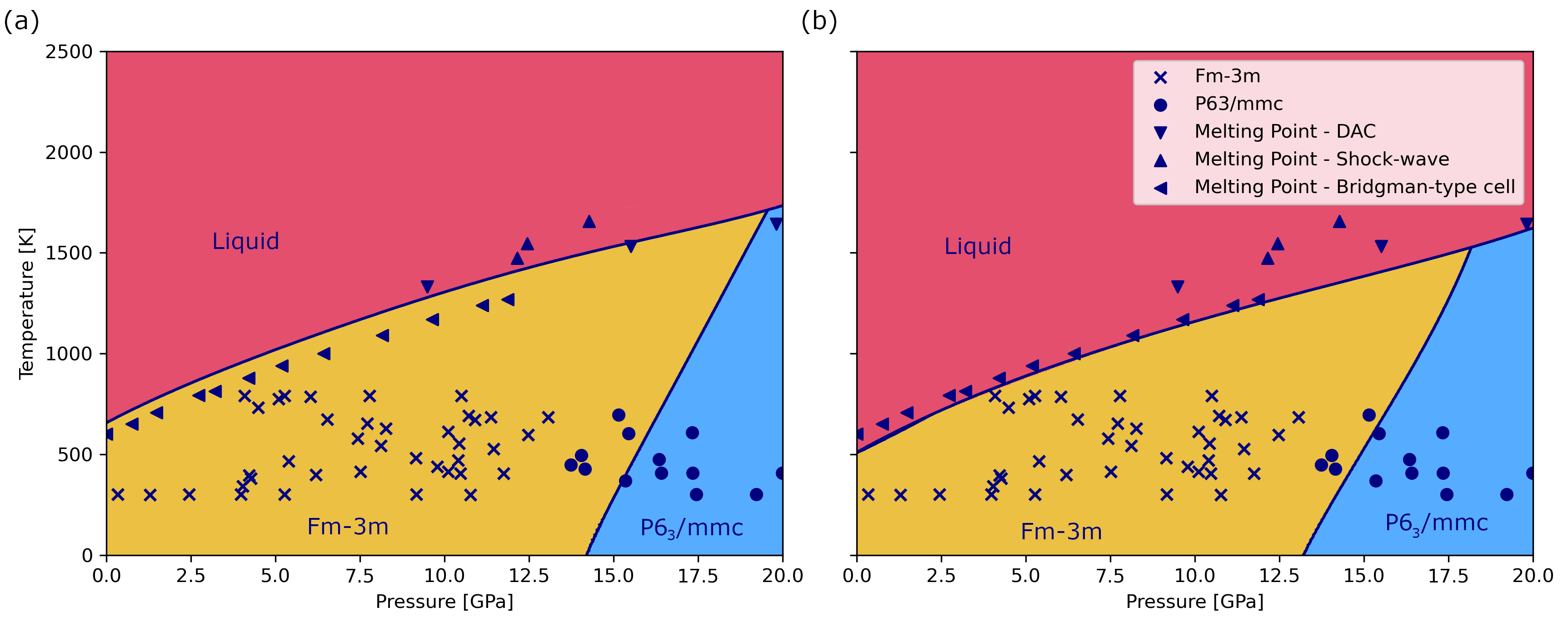
Figure 7: Phase diagram of Pb up to $20$ GPa and $2500$ K, calculated using EDDPs trained on DFT data (a) without and (b) with SOC. The symbols indicate experimental data obtained from a variety of sources. The data for the fcc and hcp phases are taken from Kuznetsov et al ¹²⁹. For the melting curve, the DAC data are from Godwal et al. ¹¹⁶, the shock-wave data from Partouche-Sebban et al. ¹¹⁷, and the Bridgman cell data from Errandonea ¹¹⁸.

The phase diagram was computed beginning with static-lattice enthalpies for the fcc and hcp phases, calculated in $1$ GPa steps from $0$ to $20$ GPa. For the relaxed structures at each of these pressures, a harmonic phonon calculation was then carried out. Thermal expansion was accounted for using the quasi-harmonic approximation (QHA) ^{130; 131}. This process requires at least several dozen phonon calculations. At the DFT level of theory, a single phonon calculation of the requisite quality would take hours of wallclock time on a CPU node. Using the EDDP, all calculations are completed in a matter of minutes.

The melting points (T${}_{\text{m}}$) are calculated using the coexistence molecular dynamics method ^{132; 133; 134; 135}. Simulation cells containing $1000$ ‘solid’ and $1000$ ‘molten’ atoms are used. Their motion is simulated using NpH molecular dynamics at pressure steps of $2.5$ GPa, covering again the pressure range from $0$ to $20$ GPa. The runs are allowed to equilibrate, and the temperature is then averaged over at least $75$ ps. The melt curve is interpolated between these explicit calculations using a polynomial fit.

Fig. 7 shows the pressure-temperature phase diagram of lead (a) without and (b) with SOC, including experimental data from a variety of sources ^{116; 117; 118; 129}. In both cases the P-T trends of the phase boundaries are in good agreement with available data. Including SOC causes a shift in the transition temperatures and pressures: $T_{m}$ is decreased by $\sim 100$ K and the fcc $\rightarrow$ hcp transition pressure is decreased by $\sim 2$ GPa.

For $T_{m}$, this leads to better agreement with the Bridgman-type cell melting point measurements of Errandonea ¹¹⁸ (the most modern experimental data available). The reduction of $T_{m}$ when SOC is taken into account arises from the softening of the phonon modes ^{136; 137}. This relationship is more pronounced with the EDDP than with DFT (Fig. 6), suggesting the SOC-induced shift in $T_{m}$ is likely overestimated with the EDDP. The EDDP overestimates the experimental fcc $\rightarrow$ hcp transition pressure in both cases, but the disparity is reduced to $\sim 1$ GPa with SOC included. The fcc-hcp-liquid triple point is located at around 18.1 GPa and 1528 K. This exceeds the estimate of Errandonea, who places the triple point at 15 GPa and 1480 K ¹¹⁸.

In summary, an EDDP has been generated that can successfully cover the pressure range from $0$ to $50$ GPa in lead. The potential gives phonon dispersions in qualitative agreement with experiment and DFT, but at specific $\mathbf{k}$-points fails to capture all of the electronic structure effects seen in DFT. Vibrational energies are nevertheless reproduced with errors of less than $5$ meV/atom for the fcc crystal even at $2000$ K. Relative errors are around $1$%. The reduction in computational cost offered by the EDDP compared to DFT allows for prediction of the phase diagram of lead in the $0$ to $20$ GPa pressure range. The coexistence MD required the EDDP, trained only on a variety of small crystal structures, to adequately describe $1000$-atom solid phases, the liquid, and the interaction between the two. The resulting melting curve is in good agreement with experiment.

V.3 Binaries: Scandium Hydride

Superhydrides have garnered substantial interest due to their intriguing characteristics, including high temperature superconductivity and hydrogen diffusivity ¹³⁸. A prominent example is LaH₁₀, which has been shown in experiment to exhibit a superconducting critical temperature above 260 K at 200 GPa ^{139; 140; 61} and is predicted to have a high hydrogen diffusion coefficient of 1.7 x 10⁴ cm²/s at 170 GPa and 1500 K^{141; 142}.

Structure prediction has played an important role in the superhydride story. In fact, silane was the first system studied with AIRSS ⁵¹, followed shortly by aluminium hydride ¹⁴³. In recent years, almost the entire periodic table of binary hydrides have been the target of a structure search ¹³⁸, saturating what can be found using ab-initio searches. These studies are often limited partly by the relatively small system sizes accessible using DFT and partly by the limited number of structures calculated during the searches - Have we truly found the minimum energy structure? The lack of certainty with which we can answer this question is perhaps indicated by the discrepancy between the large number of predicted superconducting hydrides and the small number that have been successfully synthesised. To overcome this limitation, larger systems must be explored adequately. A recent structure search on silane with up to 16 f.u. identified a new low enthalpy Pa-3 silane structure, which is not accessible with small-system searches. This highlights the importance of exploring larger systems to identify the true minimum energy structure ²². Here, we demonstrate how EDDPs can be used to accelerate these searches, include larger unit cells and sample more stoichiometries.

Scandium hydride has been subject to ab initio searches and several stable structures have been predicted, including ScH₉ which has a $T_{c}$ above 160 K at 300 GPa ¹⁴⁴. We train a single EDDP to cover a range of pressures and stoichiometries. We then use this potential to search a wider range of stoichiometries and larger unit cells to rediscover these stable structures. We demonstrate that a refined potential can be used for MD simulations of ScH₁₂, which exhibits superionicity.

Table 5 summarises the training parameters used to generate the Sc-H potential. A key step in generating EDDPs for binaries is to include a diverse range of stoichiometries in the training data. In this case stoichiometries of Sc_xH_y, where x = $1$-$4$ and y = $0$-$20$, were included in the dataset with the distribution shown in Fig. 8.

Figure 8: Distribution of structures in the scandium hydride training data; by (a) number of atoms in the unit cell and (b) Distribution of stoichiometries in the dataset.

During iterative training, local minima structures are found and included in the training data. However, the potential can often find structures multiple times — particularly if the surrounding energy basin is large — leading to over-fitting and poor transferability. To account for this, only local minima with an ensemble deviation greater than 0.02 eV/atom are added to the dataset. With this constraint, each iteration provides new environments to the training data, improving the potential. Fig. 8 shows the resulting distribution of structures in the training data in terms of both their number of atoms and their stoichiometries. The range of stoichiometries and system sizes generated during training is similar to the range used in ab initio searches of binary systems. However, with our method, DFT geometry optimisations are not required. The structures are relaxed entirely using EDDPs. In this way, an AIRSS search is performed during training, with no DFT geometry optimisations.

V.3.1 Structure Search

Searching with EDDPs can be carried out using the following three-step procedure: searching with the potential to generate a large number of structures, screening the best structures, and finally performing full DFT geometry optimisations to arrive at DFT ground states.

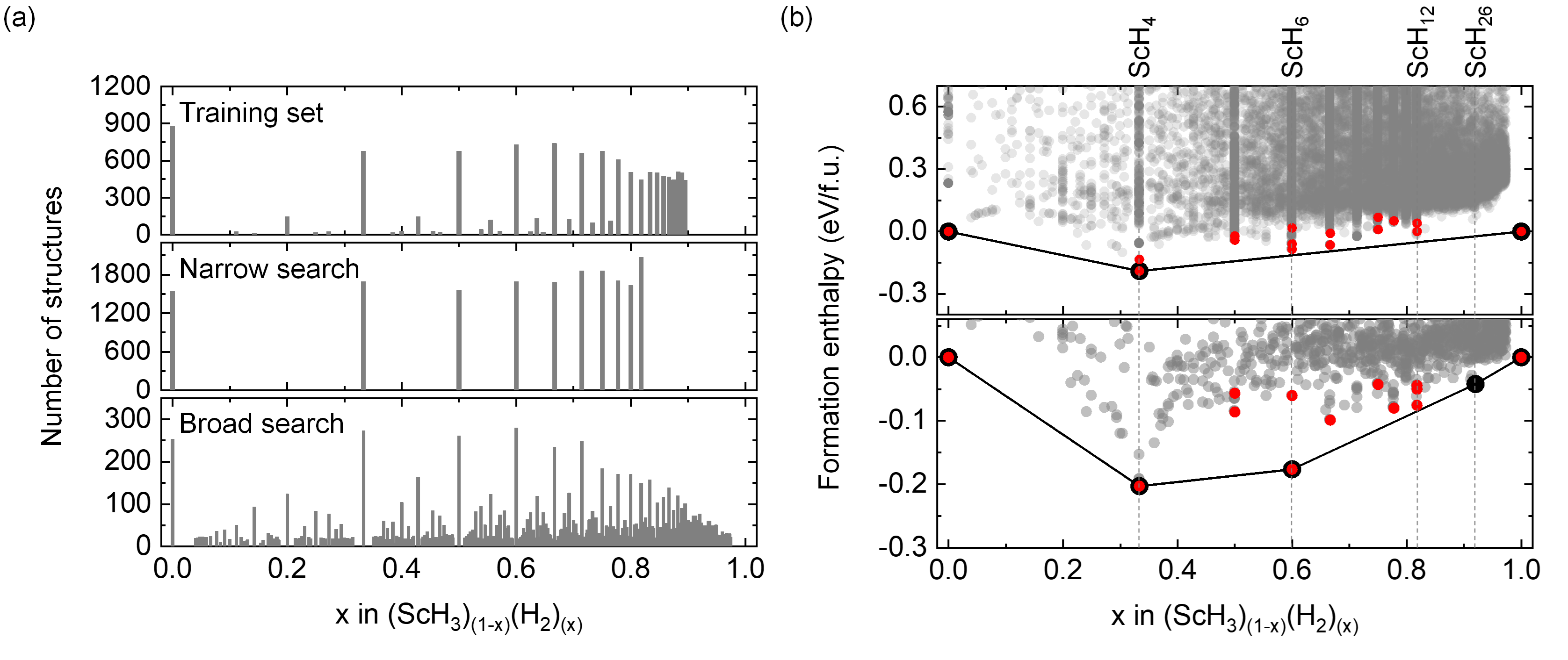
Figure 9: (a) Stoichiometry distributions of the training dataset and local minimum structures obtained from narrow and broad structure searches. (b) Convex hull diagram of scandium hydride constructed based on (top) DFT single point energies for structures searched at 250 GPa and (bottom) DFT-relaxed structures. Formation enthalpies are calculated with respect to ScH₃ and solid H₂. Black dots represent stable phases on the convex hull, gray dots represent phases above the convex hull, and red dots represent previously reported structures or similar structures that have been rediscovered.

To search with this potential, we first use AIRSS and repose to search for structures containing Sc_xH_y where x = $1$ and y = $1$-$12$ with 1-4 f.u. for a deep, narrow search and x = $1$-$8$ and y = $1$-$80$ for a broad search at 250 GPa. We used the same constraints in volumes and atomic separation for searching as we did for training (listed in table 5) but with an additional constraint of between 1 and 48 randomly chosen symmetry operations. This resulted in 39645 local minimum structures. We emphasise here that many stoichiometries in the broad structure search were not present in the training data and had not previously been accessible using DFT, as shown in Fig. 9(a).

For screening, single-point DFT calculations are performed on structures. We then re-rank the structures based on DFT enthalpies at 250 GPa, which shows reasonable – but not perfect – agreement with the energy rankings from the EDDP. Consistent rankings are not important here, so long as all the relevant structures are low enough in energy to be carried forward to this stage. Finally, structures which remain within an enthalpy window of 0.01 eV/atom after the re-ranking are retained for a full geometry optimisation. This typically does not require many optimisation steps since the structure is already close to the energy minimum.

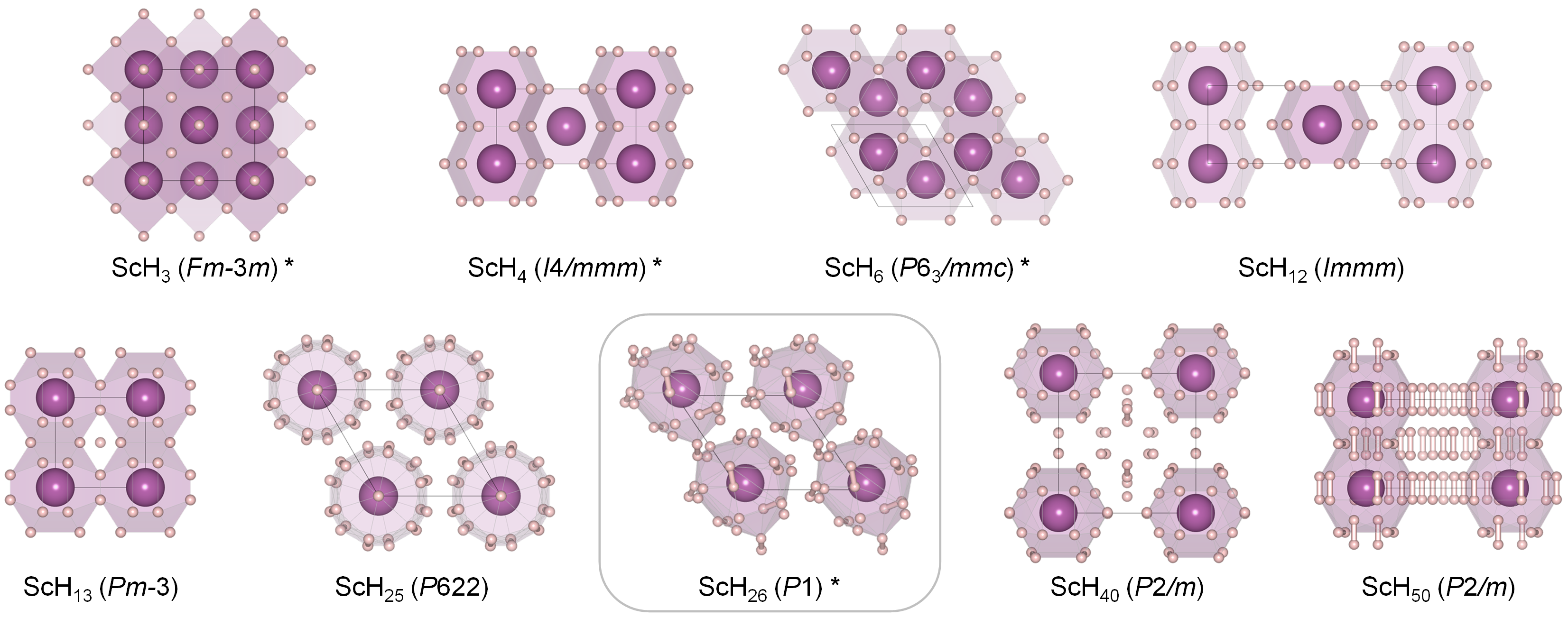
Figure 10: Stable and metastable superhydride structures. The first row includes some rediscovered structures previously reported. The second row includes some previously unreported superhydride structures that have been identified in a broad structure search. An asterisk indicates the structure is on the convex hull. The gray box indicates the unreported superhydride structure on the convex hull.

By this procedure, many previously reported scandium hydride structures were rapidly rediscovered. In Fig. 9(b) we plot the resulting convex hull where we see that Fm-3m ScH₃, I4/mmm ScH₄, and P6₃/mmc ScH₆ are stable at 250 GPa. These results are in agreement with the findings of Ye et al.¹⁴⁴. Additionally, our extensive broad search has identified a previously unreported superhydride on the hull, ScH₂₆, highlighted in Fig. 10. Finite-difference phonon calculations at the DFT level confirmed the dynamical stability of this structure on a $3\times 3\times 3$ $\mathbf{q}$-point grid.

V.3.2 Superionicity

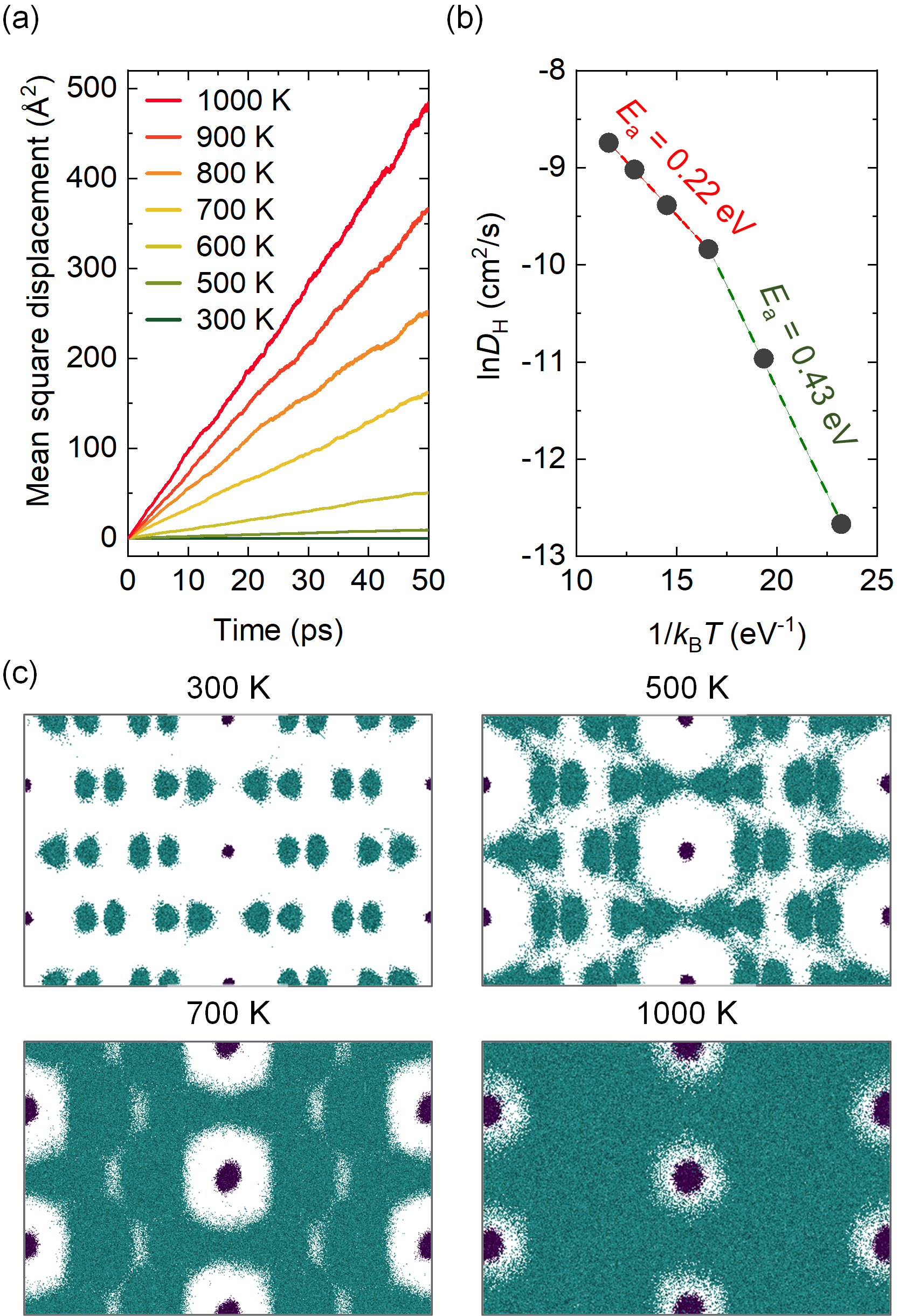
Figure 11: Hydrogen diffusion in Immm ScH₁₂ at 350 GPa. (a) Mean square displacement of hydrogen atoms at different temperatures. (b) Diffusion coefficient as a function of inverse temperature. (c) Diffusion path of hydrogen for 50 ps at 300, 500, 700, and 1000 K. Green and purple lines correspond to the trajectories of hydrogen and scandium, respectively.

Immm ScH₁₂ is one of the stable superhydrides above 325 GPa¹⁴⁴. To further explore the hydrogen diffusion in the Sc-H system using MD, we generated a refined EDDP, targeting a single stoichiometry with Immm ScH₁₂ and C2/c H₂ as marker structures. The refinement process involved adding 2000 Immm ScH₁₂ structures and 2000 C2/c H₂ structures to the training dataset with the atoms randomly perturbed by an amplitude of 0.2 Å. Additionally, the unit cell vectors are scaled by randomly chosen factors between -0.02 and +0.02.

We used ramble to carry out MD simulations on nearly-cubic supercells containing around 600 atoms using the method described in section IV.2. The simulations were performed for 60 ps at temperatures of 300, 500, 600, 700, 800, 900, and 1000 K, and a pressure of 350 GPa. The diffusion of hydrogen was analyzed for the last 50 ps of each trajectory.

At 300 K, both Sc and H atoms vibrate around their mean positions without any diffusion occurring during the 60 ps simulation timescale. The H atoms begin diffusing at $500$ K. We calculated the mean square displacement (MSD) averaged over all H atoms <$\Delta r^{2}$>. As shown in Fig. 11(a), hydrogen atoms become increasingly diffusive with temperature. The diffusion coefficient of hydrogen $D_{\textnormal{H}}$ was then calculated based on the Einstein relation <$\Delta r^{2}$> = 6$D_{\textnormal{H}}t$, assuming a three-dimensional random walk. We obtain a value of $D=$ $3.2\times 10^{-6}\ \text{cm}^{2}/\text{s}$ at 500 K, which increases to $1.6\times 10^{-4}\ \text{cm}^{2}/\text{s}$ at 1000 K.

Based on the temperature dependent diffusion coefficients shown in Fig. 11(b), the activation energy $E_{a}$ of hydrogen diffusion was estimated by fitting the data to the Arrhenius equation

$$D_{\textnormal{H}}=D_{0}e^{-E_{a}/k_{B}T}$$ (10)

The analysis of temperature-dependent diffusion coefficients reveals the manifestation of Non-Arrhenius behavior in ScH₁₂, akin to observations in other superionic conductors^{145; 146; 147}. Notably, two distinct regimes with an approximate transition temperature of 700 K are observed. Below 700 K, hydrogen atoms begin to move between lattice sites and $E_{a}=0.43$ eV. Above 700 K, $E_{a}=0.22$ eV as the hydrogen sub-lattice melts. These regimes can be differentiated in the trajectories in Fig. 11(c). In the sub-lattice melting regime, the activation energy is significantly lower, particularly when compared to LaH₁₀, which after sub-lattice melting has an activation energy of 0.44 eV above 1000 K (albeit at a lower pressure of 163 GPa) ¹⁴².

We have demonstrated that a single potential can predict stable structures across a wider range of stoichiometries than typically searched with DFT and rediscover the known phases. Refinement of this potential allows for molecular dynamics at larger length- and time-scales than previous work, leading to a prediction of a two-stage superionic transition; from site hopping to sub-lattice melting.

V.4 Ternaries: Zinc Cyanide

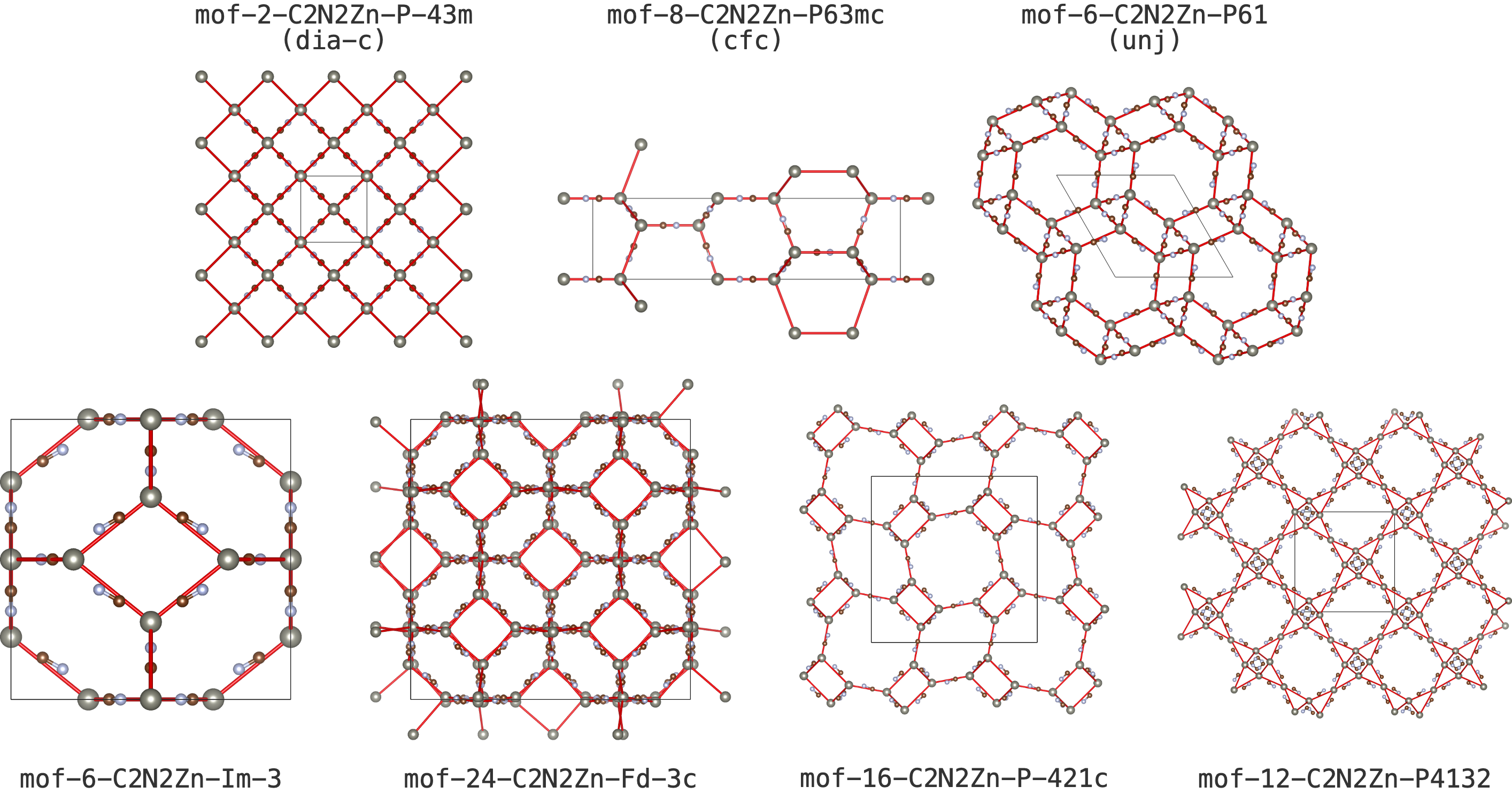
Figure 12: Crystal structures of Zn(CN)₂ polymorphs. The top row includes some previously calculated polymorphs and the second row includes low energy structures found by structure search using EDDPs.

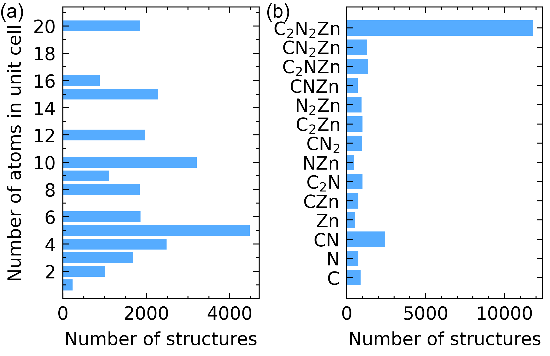
Figure 13: Distribution of structures in the Zn(CN)₂ training data; by (a) number of atoms in the unit cell and (b) stoichiometry.

MOFs are a class of materials with a wide range of potential applications from hydrogen storage to drug delivery systems. They consist of metal ions connected to organic molecular ‘linkers’ in often very complex, low-density, structures with large unit cells, making them difficult to study using plane-wave DFT. MOFs, therefore, are a difficult but desirable system to model using machine-learned potentials. Here, we choose a chemically simple MOF, zinc cyanide, which contains three elements, to demonstrate the use of EDDPs in such systems.

Zinc cyanide, Zn(CN)₂, has a disordered cubic crystal structure, with Zn atoms connected tetrahedrally by CN ‘linkers’ ¹⁴⁸. The ordered approximation of the structure is analogous to two interpenetrated diamond-like sublattices, hereon labelled ‘dia-c’ (see Fig. 12). Notably, this structure of Zn(CN)₂ possesses a large negative thermal expansion with a coefficient¹⁴⁹ $\alpha=\frac{1}{V}\frac{dV}{dT}=-17\times 10^{-6}$ K^-1, which has been attributed to the population of low-energy phonons ¹⁵⁰.

Other polymorphs of Zn(CN)₂ have been synthesised in the presence of methanol-ethanol-water mixtures under pressure ¹⁵¹. The small solvent molecules are are able to fill the vacancies formed by lower density Zn(CN)₂ structures like diamond and Lonsdaleite (dia, lon) which form at higher pressure. These structures, along with several ‘hand-crafted’ zeolitic structures, have been modeled using an empirical force-field potential ¹⁵² to study thermal expansion ¹⁵³.

In this example, we will reproduce these results without any assumed prior knowledge of the structure of Zn(CN)₂ or any polymorphs, by first searching for low-energy, low density Zn(CN)₂ structures, which could in principle be synthesised with other solvents. We then calculate the thermal expansion of these empty frameworks using molecular dynamics. We show that a general ‘all purpose’ Zn + 2C + 2N potential can be used for structure searching and for molecular dynamics with reasonable accuracy.

V.4.1 Training

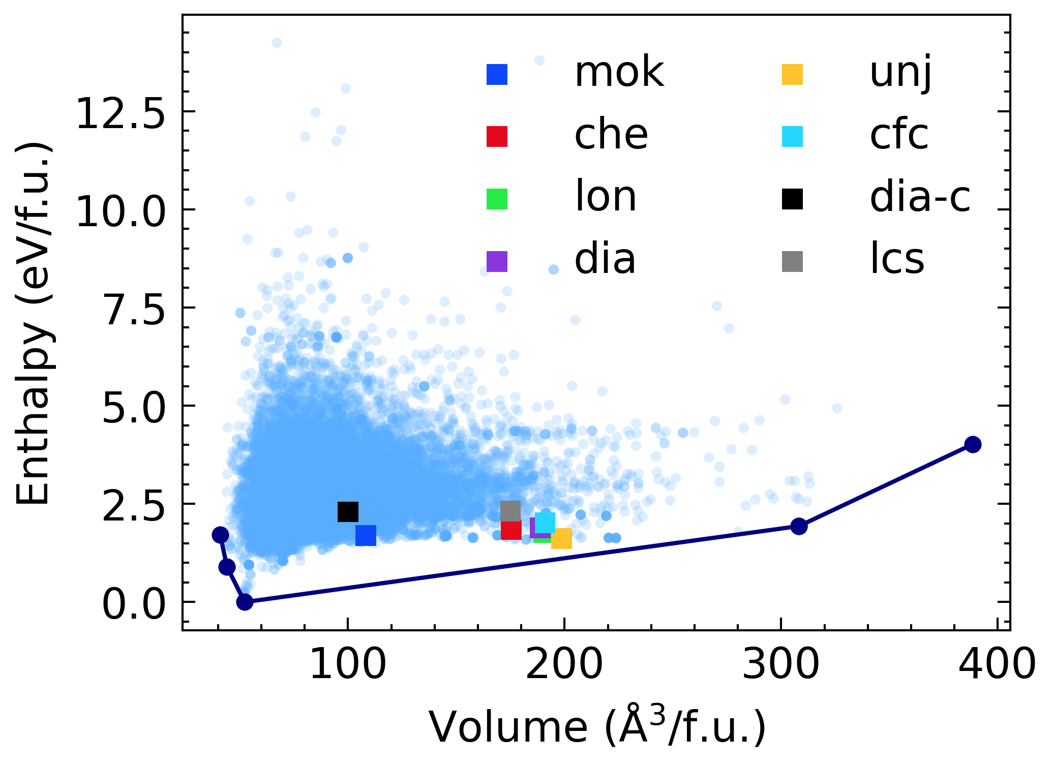
Figure 14: Range of volume - enthalpy values for structures found by random structure search with the Zn(CN)₂ EDDP. Square symbols indicate the named structure types.

Training potentials for ternary compositions can be more difficult than for a single species or binaries; the combinatoric variation of the local environment requires exponentially longer feature vectors — they contain 498 components in this case, in contrast with 43 in lead and 172 in scandium hydride — and significantly more training data. We retain the principle of training potentials on small unit cells. We further emphasise a distinction between the local stoichiometry — the atoms contained within a cut-off radius — and the global stoichiometry of the crystal. Hence, for small-cell training, the variety of the training data can be enhanced by sampling structures with relatively few atoms, but with a range of global stoichiometries.

In this case, the training data consists of Zn_lC_mN_n where $l=0,1$, $m=0,1,2$, $n=0,1,2$, with a weighting towards $l=1$, $m=2$, $n=2$, and up to 4 f.u. per cell. The resulting distribution of data is shown in Fig. 13. Table 5 summarises the training parameters used to generate the Zn(CN)₂ potential. Similarly to the carbon example, longer-range dispersion effects are implicitly incorporated in the generation of EDDPs by including them in the DFT dataset.

V.4.2 Results

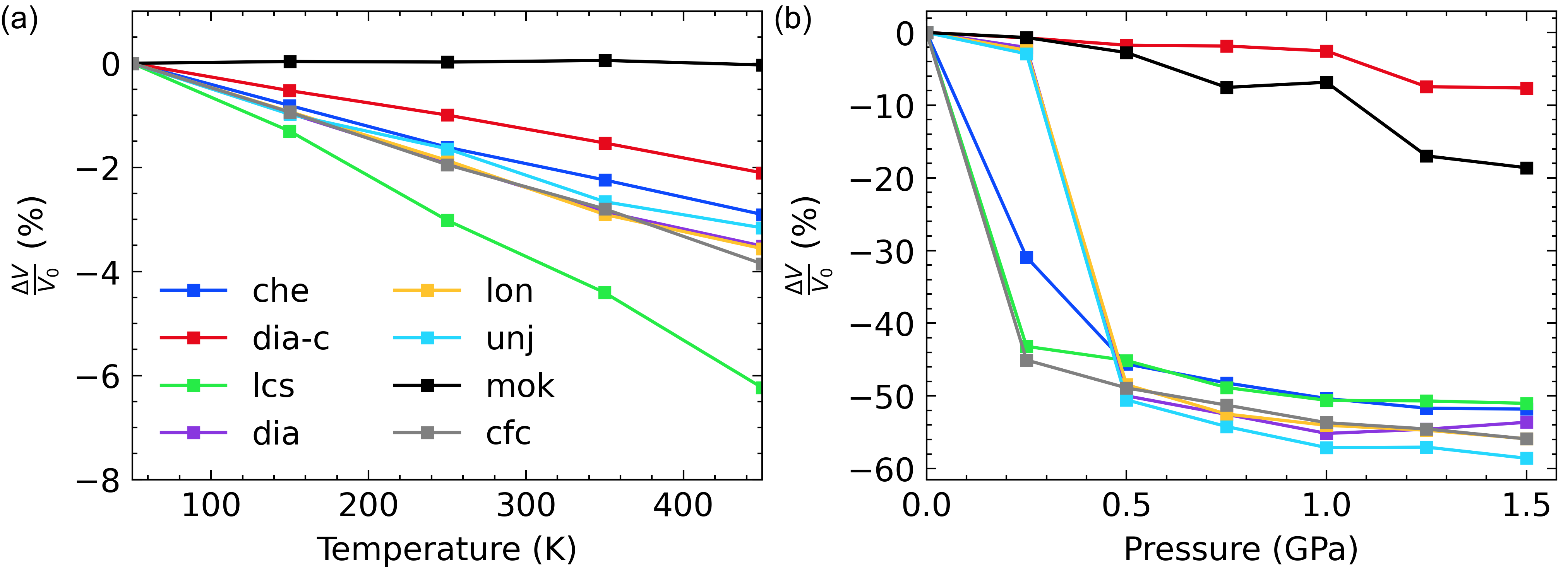
Figure 15: Relative volume change with temperature at 0 GPa (a) and with pressure at 300 K (b) for a range of metastable and hypothetical Zn(CN)₂ structures.

Table 8: Thermal expansion coefficients for the structures shown in Fig. 15, calculated with TS and MBD dispersion corrections. Experimental values¹⁵³, where available, are in parenthesis.

ID	label	$\alpha^{\text{MBD}}$ ($10^{-6}$ K-1)	$\alpha^{\text{TS}}$ ($10^{-6}$ K-1)
mof-152-C2N2Zn-I213	che	-20.66	-24.88
mof-2-C2N2Zn-P-43m	dia-c	-14.21 (-17.46)	-17.26 (-17.46)
mof-24-C2N2Zn-I-43d	lcs	-30.68	-50.57
mof-24-C2N2Zn-R3m	dia	-25.33	-30.46
mof-4-C2N2Zn-P63mc	lon	-25.58	-30.70
mof-6-C2N2Zn-P61	unj	-21.90	-27.66
mof-8-C2N2Zn-Cc	mok	2.04	0.13
mof-8-C2N2Zn-P63mc	cfc	-25.72	-31.84

We begin by performing a random structure search with the EDDP, using AIRSS and repose, generating around 40,000 Zn(CN)₂ structures with a target volume between 100 and 300 ų/f.u., with each containing between 1 and 20 f.u. and 1-48 symmetry operations. Fig. 14 shows these structures’ enthalpy-volume distribution. We find a high concentration of points below 100 ų/f.u., which have a higher density than is typical for a Zn(CN)₂ framework. These are structures which, despite being initialised with large unit cells, condensed into much denser phases during geometry optimisation. This demonstrates a difficulty with low-density structure prediction, as there are several accessible routes to condensed states, but much fewer routes to low-density phases. With EDDP structure searching, we can overcome this issue simply by performing very extensive searches. This is also a demonstration of the transferability of the EDDP, which — in contrast to an empirically derived potential — is able to describe the layered hexagonal and tetrahedral carbon nitride-like environments typical of the condensed phases.

Several low-density zeolite-like structures were predicted in the search. We were able to rediscover the polymorphs proposed by Trousselet et al. (which are indicated by squares in Fig. 14) as low-energy states close to the enthalpy-volume convex hull. We also find several other novel stable polymorphs with similar volumes and energies, the structures of which are shown in Fig. 12. These new structures include some which are similar to known clathrate types (mof-6-C2N2Zn-Im-3 and mof-24-C2N2Zn-Fd-3c) and other novel complex networks (such as mof-16-C2N2Zn-P-421c and mof-12-C2N2Zn-P4132).

We then explored the the behaviour of some of the low-density polymorphs at finite temperature. Specifically, we used the structures calculated by Trousselet et al. with the labels che, dia-c, lcs, dia, lon, unj, mok and cfc. These are tabulated, along with their structure ID, in table 8.

We used ramble to run MD at 50, 150, 250, 350, 450 K at ambient pressure with supercells containing around 500 atoms. These supercells were made to be ‘nearly-cubic’ using the method described in section IV.2. Fig. 15(a) shows volume change with temperature for these structures. Linear fits to the data show an expansion coefficient, $\alpha=-17.26\times 10^{-6}$ K^-1 for the ‘dia-c’, which is remarkably close to the experimental and previously calculated values of -17.4 and -16.9 $\times 10^{-6}$ K^-1 respectively. A second potential trained using the MBD dispersion correction scheme¹⁵⁴ gave qualitatively similar results, as shown in table 8, but a value of $\alpha=-14.21\times 10^{-6}$ K^-1. The behaviour of the metastable hypothetical structures is in good agreement with those calculated using a parameterised force-field¹⁵³.

We also ran MD simulations at $300$ K for a range of pressures. The volume changes are shown in Fig. 15(b). We see that the denser structures, dia-c and mok, remain stable, whereas the more open structures undergo a structural transition above 0.25 GPa. This is also in line with results obtained by Trousselet et al..

With this example, we highlight the feasibility of generating a good potential for a ternary system and extracting physically sensible results. We should note that in calculating the thermal expansion, a well-parameterised empirical potential is clearly sufficient to model the dynamics. However, as demonstrated by our structure search, a machine-learned potential is transferable to more unusual systems, for example with broken cyanide bonds or layered C-N networks. This means EDDPs can be exploited for exploration-based studies — where calculations can be performed on systems without any prior assumptions — to make new discoveries.

While this ternary system is feasible, typical MOFs contain more than 3 or 4 elements. Chemical complexity becomes a limiting factor for machine-learned potentials and EDDPs are no exception. The EDDP feature vector scales such that a naive extension to systems with more elements will lead to overly sparse feature vectors and a consequential bottleneck in calculation speed. Recent work by Ceriotti and co-workers has attempted to address this issue by considering ‘alchemical’ correlations ¹⁵⁵. To continue increasing the chemical complexity, it may be necessary to adopt a similar approach.

VI Conclusion

In this work, we have demonstrated that the EDDPs can significantly accelerate structure prediction, but also have applications beyond this initial intent. This is achieved without requiring a sophisticated (and costly) neural network architecture and relies only on single-point DFT energy calculations of small cells, making them convenient and cheap to train. The EDDPs’ smoothness means they are well-behaved over wide regions of structure space. They possess a good degree of size transferability, allowing potentials trained on cells containing $24$ atoms or less to model much larger systems successfully. For pure elements, only a few thousand DFT calculations on small cells are required to achieve meV-level accuracy, excepting carbon, a particularly difficult system.

In the cases of both scandium hydride and zinc cyanide, a single EDDP each is capable of successfully searching a wide range of stoichiometries. This is evidenced by the reproduction of known results in these two test cases. An EDDP-enabled MD simulation of Immm-ScH₁₂ predicts hydrogen sublattice melting and superionicity above $700$ K at $350$ GPa. This phenomenon has been demonstrated using AIMD for other superhydrides under high pressure. By combining high-throughput phonon calculations and coexistence MD, an EDDP was used to generate a phase diagram for lead. This was done taking SOC into account, which brings the melt curve into better agreement with experiment.

The EDDPs were originally termed ‘ephemeral’ to indicate the intention to design a custom potential suitable for a given application and then discard it. Instead of expending considerable effort and computational power training a ‘perfect’ potential, it can be preferable to train a sufficient potential and spend the available resources on using it.

This philosophy has not entirely been superseded - our intent is not to present a new set of benchmark potentials for the systems discussed. Nevertheless, the ease with which EDDPs can be trained means that for a given application, often several dozen potentials can be generated in order to assess the best combination of parameters. Furthermore, once a satisfactory potential has been generated, the robust nature and smoothness of the EDDPs means they are applicable more widely than originally anticipated. The ‘ephemeral’ data-derived potentials have proven more long-lived than expected.

Author Declarations

Conflict of Interest

The authors have no conflicts to disclose.

Data Availability

The data that support the findings of this study are openly available on MaterialsCloud at https://doi.org/10.24435/materialscloud:44-c5.

References

References

- Schmidt et al. (2019) J. Schmidt, M. R. G. Marques, S. Botti, and M. A. L. Marques, “Recent advances and applications of machine learning in solid-state materials science,” npj Computational Materials 5, 83 (2019).
- Kulik et al. (2022) H. J. Kulik, T. Hammerschmidt, J. Schmidt, S. Botti, M. A. L. Marques, M. Boley, M. Scheffler, M. Todorović, P. Rinke, C. Oses, A. Smolyanyuk, S. Curtarolo, A. Tkatchenko, A. P. Bartók, S. Manzhos, M. Ihara, T. Carrington, J. Behler, O. Isayev, M. Veit, A. Grisafi, J. Nigam, M. Ceriotti, K. T. Schütt, J. Westermayr, M. Gastegger, R. J. Maurer, B. Kalita, K. Burke, R. Nagai, R. Akashi, O. Sugino, J. Hermann, F. Noé, S. Pilati, C. Draxl, M. Kuban, S. Rigamonti, M. Scheidgen, M. Esters, D. Hicks, C. Toher, P. V. Balachandran, I. Tamblyn, S. Whitelam, C. Bellinger, and L. M. Ghiringhelli, “Roadmap on machine learning in electronic structure,” Electronic Structure 4, 023004 (2022).
- Bhadeshia, MacKay, and Svensson (1995) H. K. D. H. Bhadeshia, D. J. C. MacKay, and L.-E. Svensson, “Impact toughness of C–Mn steel arc welds – Bayesian neural network analysis,” Materials Science and Technology 11, 1046–1051 (1995).
- Sutton et al. (2019) C. Sutton, L. M. Ghiringhelli, T. Yamamoto, Y. Lysogorskiy, L. Blumenthal, T. Hammerschmidt, J. R. Golebiowski, X. Liu, A. Ziletti, and M. Scheffler, “Crowd-sourcing materials-science challenges with the NOMAD 2018 Kaggle competition,” npj Computational Materials 5, 111 (2019).
- Garrido Torres et al. (2021) J. A. Garrido Torres, V. Gharakhanyan, N. Artrith, T. H. Eegholm, and A. Urban, “Augmenting zero-Kelvin quantum mechanics with machine learning for the prediction of chemical reactions at high temperatures,” Nature Communications 12, 7012 (2021).
- Weinreich et al. (2022) J. Weinreich, D. Lemm, G. F. von Rudorff, and O. A. von Lilienfeld, “Ab initio machine learning of phase space averages,” The Journal of Chemical Physics 157 (2022).
- Tozer, Ingamells, and Handy (1996) D. J. Tozer, V. E. Ingamells, and N. C. Handy, “Exchange-correlation potentials,” The Journal of Chemical Physics 105, 9200–9213 (1996).
- Snyder et al. (2012) J. C. Snyder, M. Rupp, K. Hansen, K.-R. Müller, and K. Burke, “Finding density functionals with machine learning,” Phys. Rev. Lett. 108, 253002 (2012).
- Nagai, Akashi, and Sugino (2020) R. Nagai, R. Akashi, and O. Sugino, “Completing density functional theory by machine learning hidden messages from molecules,” npj Computational Materials 6, 43 (2020).
- Behler and Parrinello (2007) J. Behler and M. Parrinello, “Generalized neural-network representation of high-dimensional potential-energy surfaces,” Phys. Rev. Lett. 98, 146401 (2007).
- Bartók et al. (2010) A. P. Bartók, M. C. Payne, R. Kondor, and G. Csányi, “Gaussian approximation potentials: The accuracy of quantum mechanics, without the electrons,” Phys. Rev. Lett. 104, 136403 (2010).
- Deringer, Caro, and Csányi (2019) V. L. Deringer, M. A. Caro, and G. Csányi, “Machine learning interatomic potentials as emerging tools for materials science,” Advanced Materials 31, 1902765 (2019).
- Hohenberg and Kohn (1964) P. Hohenberg and W. Kohn, “Inhomogeneous electron gas,” Phys. Rev. 136, B864–B871 (1964).
- Kohn and Sham (1965) W. Kohn and L. J. Sham, “Self-consistent equations including exchange and correlation effects,” Phys. Rev. 140, A1133–A1138 (1965).
- Bartók et al. (2018) A. P. Bartók, J. Kermode, N. Bernstein, and G. Csányi, “Machine learning a general-purpose interatomic potential for silicon,” Phys. Rev. X 8, 041048 (2018).
- Cheng et al. (2020) B. Cheng, G. Mazzola, C. J. Pickard, and M. Ceriotti, “Evidence for supercritical behaviour of high-pressure liquid hydrogen,” Nature 585, 217–220 (2020).
- Cheng et al. (2019) B. Cheng, E. A. Engel, J. Behler, C. Dellago, and M. Ceriotti, “Ab initio thermodynamics of liquid and solid water,” Proceedings of the National Academy of Sciences 116, 1110–1115 (2019).
- Sosso et al. (2012) G. C. Sosso, G. Miceli, S. Caravati, J. Behler, and M. Bernasconi, “Neural network interatomic potential for the phase change material GeTe,” Phys. Rev. B 85, 174103 (2012).
- Mocanu et al. (2018) F. C. Mocanu, K. Konstantinou, T. H. Lee, N. Bernstein, V. L. Deringer, G. Csányi, and S. R. Elliott, “Modeling the phase-change memory material, Ge2Sb2Te5, with a machine-learned interatomic potential,” The Journal of Physical Chemistry B 122, 8998–9006 (2018).
- Thompson et al. (2015) A. Thompson, L. Swiler, C. Trott, S. Foiles, and G. Tucker, “Spectral neighbor analysis method for automated generation of quantum-accurate interatomic potentials,” Journal of Computational Physics 285, 316–330 (2015).
- Zhang et al. (2018) L. Zhang, J. Han, H. Wang, R. Car, and W. E, “Deep potential molecular dynamics: A scalable model with the accuracy of quantum mechanics,” Phys. Rev. Lett. 120, 143001 (2018).
- Pickard (2022) C. J. Pickard, “Ephemeral data derived potentials for random structure search,” Phys. Rev. B 106, 014102 (2022).
- Shapeev (2016) A. V. Shapeev, “Moment tensor potentials: A class of systematically improvable interatomic potentials,” Multiscale Modeling & Simulation 14, 1153–1173 (2016).
- Drautz (2020) R. Drautz, “Atomic cluster expansion of scalar, vectorial, and tensorial properties including magnetism and charge transfer,” Phys. Rev. B 102, 024104 (2020).
- Dusson et al. (2022) G. Dusson, M. Bachmayr, G. Csányi, R. Drautz, S. Etter, C. van der Oord, and C. Ortner, “Atomic cluster expansion: Completeness, efficiency and stability,” Journal of Computational Physics 454, 110946 (2022).
- Batatia et al. (2022) I. Batatia, D. P. Kovacs, G. Simm, C. Ortner, and G. Csanyi, “MACE: Higher order equivariant message passing neural networks for fast and accurate force fields,” in Advances in Neural Information Processing Systems, Vol. 35, edited by S. Koyejo, S. Mohamed, A. Agarwal, D. Belgrave, K. Cho, and A. Oh (Curran Associates, Inc., 2022) pp. 11423–11436.
- Musaelian et al. (2023) A. Musaelian, S. Batzner, A. Johansson, L. Sun, C. J. Owen, M. Kornbluth, and B. Kozinsky, “Learning local equivariant representations for large-scale atomistic dynamics,” Nature Communications 14, 579 (2023).
- Behler and Csányi (2021) J. Behler and G. Csányi, “Machine learning potentials for extended systems: a perspective,” The European Physical Journal B 94, 142 (2021).
- Behler (2021) J. Behler, “Four generations of high-dimensional neural network potentials,” Chemical Reviews 121, 10037–10072 (2021).
- Chen and Ong (2022) C. Chen and S. P. Ong, “A universal graph deep learning interatomic potential for the periodic table,” Nature Computational Science 2, 718–728 (2022).
- Choudhary et al. (2023) K. Choudhary, B. DeCost, L. Major, K. Butler, J. Thiyagalingam, and F. Tavazza, “Unified graph neural network force-field for the periodic table: solid state applications,” Digital Discovery 2, 346–355 (2023).
- Nigam et al. (2022) J. Nigam, S. Pozdnyakov, G. Fraux, and M. Ceriotti, “Unified theory of atom-centered representations and message-passing machine-learning schemes,” The Journal of Chemical Physics 156 (2022).
- Behler (2011) J. Behler, “Atom-centered symmetry functions for constructing high-dimensional neural network potentials,” The Journal of Chemical Physics 134 (2011), 074106.
- Bartók, Kondor, and Csányi (2013) A. P. Bartók, R. Kondor, and G. Csányi, “On representing chemical environments,” Phys. Rev. B 87, 184115 (2013).
- Willatt, Musil, and Ceriotti (2019) M. J. Willatt, F. Musil, and M. Ceriotti, “Atom-density representations for machine learning,” The Journal of Chemical Physics 150 (2019), 154110.
- Musil et al. (2021) F. Musil, A. Grisafi, A. P. Bartók, C. Ortner, G. Csányi, and M. Ceriotti, “Physics-inspired structural representations for molecules and materials,” Chemical Reviews 121, 9759–9815 (2021).
- Smith et al. (2018) J. S. Smith, B. Nebgen, N. Lubbers, O. Isayev, and A. E. Roitberg, “Less is more: Sampling chemical space with active learning,” The Journal of Chemical Physics 148 (2018).
- Novikov et al. (2020) I. S. Novikov, K. Gubaev, E. V. Podryabinkin, and A. V. Shapeev, “The MLIP package: moment tensor potentials with MPI and active learning,” Machine Learning: Science and Technology 2, 025002 (2020).
- Miksch et al. (2021) A. M. Miksch, T. Morawietz, J. Kästner, A. Urban, and N. Artrith, “Strategies for the construction of machine-learning potentials for accurate and efficient atomic-scale simulations,” Machine Learning: Science and Technology 2, 031001 (2021).
- Podryabinkin and Shapeev (2017) E. V. Podryabinkin and A. V. Shapeev, “Active learning of linearly parametrized interatomic potentials,” Computational Materials Science 140, 171–180 (2017).
- Zhang et al. (2019) L. Zhang, D.-Y. Lin, H. Wang, R. Car, and W. E, “Active learning of uniformly accurate interatomic potentials for materials simulation,” Phys. Rev. Mater. 3, 023804 (2019).
- van der Oord et al. (2023) C. van der Oord, M. Sachs, D. P. Kovács, C. Ortner, and G. Csányi, “Hyperactive learning for data-driven interatomic potentials,” (2023).
- Kulichenko et al. (2023) M. Kulichenko, K. Barros, N. Lubbers, Y. W. Li, R. Messerly, S. Tretiak, J. S. Smith, and B. Nebgen, “Uncertainty-driven dynamics for active learning of interatomic potentials,” Nature Computational Science 3, 230–239 (2023).
- Dolgirev, Kruglov, and Oganov (2016) P. E. Dolgirev, I. A. Kruglov, and A. R. Oganov, “Machine learning scheme for fast extraction of chemically interpretable interatomic potentials,” AIP Advances 6, 085318 (2016).
- Hajinazar, Shao, and Kolmogorov (2017) S. Hajinazar, J. Shao, and A. N. Kolmogorov, “Stratified construction of neural network based interatomic models for multicomponent materials,” Phys. Rev. B 95, 014114 (2017).
- Hajinazar et al. (2021) S. Hajinazar, A. Thorn, E. D. Sandoval, S. Kharabadze, and A. N. Kolmogorov, “MAISE: Construction of neural network interatomic models and evolutionary structure optimization,” Computer Physics Communications 259, 107679 (2021).
- Deringer, Pickard, and Csányi (2018) V. L. Deringer, C. J. Pickard, and G. Csányi, “Data-driven learning of total and local energies in elemental boron,” Phys. Rev. Lett. 120, 156001 (2018).
- Deringer et al. (2018) V. L. Deringer, D. M. Proserpio, G. Csányi, and C. J. Pickard, “Data-driven learning and prediction of inorganic crystal structures,” Faraday Discuss. 211, 45–59 (2018).
- Oganov et al. (2019) A. R. Oganov, C. J. Pickard, Q. Zhu, and R. J. Needs, “Structure prediction drives materials discovery,” Nature Reviews Materials 4, 331–348 (2019).
- Conway, Pickard, and Hermann (2023) L. J. Conway, C. J. Pickard, and A. Hermann, “3.12 - first principles crystal structure prediction,” in Comprehensive Inorganic Chemistry III (Third Edition), edited by J. Reedijk and K. R. Poeppelmeier (Elsevier, Oxford, 2023) 3rd ed., pp. 393–420.
- Pickard and Needs (2006) C. J. Pickard and R. J. Needs, “High-pressure phases of silane,” Phys. Rev. Lett. 97, 045504 (2006).
- Pickard and Needs (2011) C. J. Pickard and R. J. Needs, “Ab initio random structure searching,” Journal of Physics: Condensed Matter 23, 053201 (2011).
- Glass, Oganov, and Hansen (2006) C. W. Glass, A. R. Oganov, and N. Hansen, “USPEX—evolutionary crystal structure prediction,” Computer Physics Communications 175, 713–720 (2006).
- Lonie and Zurek (2011) D. C. Lonie and E. Zurek, “XtalOpt: An open-source evolutionary algorithm for crystal structure prediction,” Computer Physics Communications 182, 372–387 (2011).
- Wang et al. (2010) Y. Wang, J. Lv, L. Zhu, and Y. Ma, “Crystal structure prediction via particle-swarm optimization,” Phys. Rev. B 82, 094116 (2010).
- Wales and Doye (1997) D. J. Wales and J. P. K. Doye, “Global optimization by basin-hopping and the lowest energy structures of Lennard-Jones clusters containing up to 110 atoms,” The Journal of Physical Chemistry A 101, 5111–5116 (1997).
- Pickard and Needs (2007a) C. J. Pickard and R. J. Needs, “Structure of phase III of solid hydrogen,” Nature Physics 3, 473–476 (2007a).
- Pickard and Needs (2010) C. J. Pickard and R. J. Needs, “Aluminium at terapascal pressures,” Nature Materials 9, 624–627 (2010).
- Liu et al. (2020) C. Liu, H. Gao, A. Hermann, Y. Wang, M. Miao, C. J. Pickard, R. J. Needs, H.-T. Wang, D. Xing, and J. Sun, “Plastic and superionic helium ammonia compounds under high pressure and high temperature,” Phys. Rev. X 10, 021007 (2020).
- Duan et al. (2014) D. Duan, Y. Liu, F. Tian, D. Li, X. Huang, Z. Zhao, H. Yu, B. Liu, W. Tian, and T. Cui, “Pressure-induced metallization of dense (H2S)2H2 with high-Tc superconductivity,” Scientific Reports 4, 6968 (2014).
- Peng et al. (2017) F. Peng, Y. Sun, C. J. Pickard, R. J. Needs, Q. Wu, and Y. Ma, “Hydrogen clathrate structures in rare earth hydrides at high pressures: Possible route to room-temperature superconductivity,” Phys. Rev. Lett. 119, 107001 (2017).
- Liu et al. (2017) H. Liu, I. I. Naumov, R. Hoffmann, N. W. Ashcroft, and R. J. Hemley, “Potential high-Tc superconducting lanthanum and yttrium hydrides at high pressure,” Proceedings of the National Academy of Sciences 114, 6990–6995 (2017).
- Ouyang, Xie, and Jiang (2015) R. Ouyang, Y. Xie, and D.-e. Jiang, “Global minimization of gold clusters by combining neural network potentials and the basin-hopping method,” Nanoscale 7, 14817–14821 (2015).
- Deringer, Csányi, and Proserpio (2017) V. L. Deringer, G. Csányi, and D. M. Proserpio, “Extracting crystal chemistry from amorphous carbon structures,” ChemPhysChem 18, 873–877 (2017).
- Patra et al. (2017) T. K. Patra, V. Meenakshisundaram, J.-H. Hung, and D. S. Simmons, “Neural-network-biased genetic algorithms for materials design: Evolutionary algorithms that learn,” ACS Combinatorial Science 19, 96–107 (2017).
- Tong et al. (2018) Q. Tong, L. Xue, J. Lv, Y. Wang, and Y. Ma, “Accelerating CALYPSO structure prediction by data-driven learning of a potential energy surface,” Faraday Discuss. 211, 31–43 (2018).
- Podryabinkin et al. (2019) E. V. Podryabinkin, E. V. Tikhonov, A. V. Shapeev, and A. R. Oganov, “Accelerating crystal structure prediction by machine-learning interatomic potentials with active learning,” Phys. Rev. B 99, 064114 (2019).
- Gubaev et al. (2019) K. Gubaev, E. V. Podryabinkin, G. L. Hart, and A. V. Shapeev, “Accelerating high-throughput searches for new alloys with active learning of interatomic potentials,” Computational Materials Science 156, 148–156 (2019).
- Thorn et al. (2019) A. Thorn, J. Rojas-Nunez, S. Hajinazar, S. E. Baltazar, and A. N. Kolmogorov, “Toward ab initio ground states of gold clusters via neural network modeling,” The Journal of Physical Chemistry C 123, 30088–30098 (2019).
- Bisbo and Hammer (2020) M. K. Bisbo and B. Hammer, “Efficient global structure optimization with a machine-learned surrogate model,” Phys. Rev. Lett. 124, 086102 (2020).
- Kaappa, del Río, and Jacobsen (2021) S. Kaappa, E. G. del Río, and K. W. Jacobsen, “Global optimization of atomic structures with gradient-enhanced gaussian process regression,” Phys. Rev. B 103, 174114 (2021).
- Dasenbrock-Gammon et al. (2023) N. Dasenbrock-Gammon, E. Snider, R. McBride, H. Pasan, D. Durkee, N. Khalvashi-Sutter, S. Munasinghe, S. E. Dissanayake, K. V. Lawler, A. Salamat, and R. P. Dias, “Evidence of near-ambient superconductivity in a N-doped lutetium hydride,” Nature 615, 244–250 (2023).
- Xie et al. (2023) F. Xie, T. Lu, Z. Yu, Y. Wang, Z. Wang, S. Meng, and M. Liu, “Lu–H–N Phase Diagram from First-Principles Calculations,” Chinese Physics Letters 40, 057401 (2023).
- Huo et al. (2023) Z. Huo, D. Duan, T. Ma, Z. Zhang, Q. Jiang, D. An, H. Song, F. Tian, and T. Cui, “First-principles study on the conventional superconductivity of N-doped fcc-LuH3,” Matter and Radiation at Extremes 8, 038402 (2023), https://pubs.aip.org/aip/mre/article-pdf/doi/10.1063/5.0151844/18116117/038402_1_5.0151844.pdf .
- Hilleke et al. (2023) K. P. Hilleke, X. Wang, D. Luo, N. Geng, B. Wang, F. Belli, and E. Zurek, “Structure, stability, and superconductivity of N-doped lutetium hydrides at kbar pressures,” Phys. Rev. B 108, 014511 (2023).
- Ferreira et al. (2023) P. P. Ferreira, L. J. Conway, A. Cucciari, S. Di Cataldo, F. Giannessi, E. Kogler, L. T. F. Eleno, C. J. Pickard, C. Heil, and L. Boeri, “Search for ambient superconductivity in the Lu-N-H system,” Nature Communications 14, 5367 (2023).
- Kim et al. (2023) S.-W. Kim, L. J. Conway, C. J. Pickard, G. L. Pascut, and B. Monserrat, “Microscopic theory of colour in lutetium hydride,” (2023), arXiv:2304.07326 [cond-mat.supr-con] .
- Clark et al. (2005) S. J. Clark, M. D. Segall, C. J. Pickard, P. J. Hasnip, M. I. J. Probert, K. Refson, and M. C. Payne, “First principles methods using CASTEP,” Zeitschrift für Kristallographie - Crystalline Materials 220, 567 – 570 (2005).
- Jones and Chapman (1924) J. E. Jones and S. Chapman, “On the determination of molecular fields.—I. from the variation of the viscosity of a gas with temperature,” Proceedings of the Royal Society of London. Series A, Containing Papers of a Mathematical and Physical Character 106, 441–462 (1924).
- Lennard-Jones (1931) J. E. Lennard-Jones, “Cohesion,” Proceedings of the Physical Society 43, 461 (1931).
- Born and Misra (1940) M. Born and R. D. Misra, “On the stability of crystal lattices. IV,” Mathematical Proceedings of the Cambridge Philosophical Society 36, 466–478 (1940).
- Wang et al. (2020) X. Wang, S. Ramírez-Hinestrosa, J. Dobnikar, and D. Frenkel, “The Lennard-Jones potential: when (not) to use it,” Phys. Chem. Chem. Phys. 22, 10624–10633 (2020).
- Schran, Brezina, and Marsalek (2020) C. Schran, K. Brezina, and O. Marsalek, “Committee neural network potentials control generalization errors and enable active learning,” The Journal of Chemical Physics 153, 104105 (2020).
- Hansen and Salamon (1990) L. Hansen and P. Salamon, “Neural network ensembles,” IEEE Transactions on Pattern Analysis and Machine Intelligence 12, 993–1001 (1990).
- Poul et al. (2023) M. Poul, L. Huber, E. Bitzek, and J. Neugebauer, “Systematic atomic structure datasets for machine learning potentials: Application to defects in magnesium,” Phys. Rev. B 107, 104103 (2023).
- Meziere et al. (2023) J. A. Meziere, Y. Luo, Y. Zia, L. Beland, M. Daymond, and G. L. W. Hart, “Accelerating training of MLIPs through small-cell training,” (2023), arXiv:2304.01314 [cond-mat.mtrl-sci] .
- Levenberg (1944) K. Levenberg, “A method for the solution of certain non-linear problems in least squares,” Quart. Appl. Math. 2, 164–168 (1944).
- Moré (1978) J. J. Moré, “The Levenberg-Marquardt algorithm: Implementation and theory,” in Numerical Analysis, edited by G. A. Watson (Springer Berlin Heidelberg, Berlin, Heidelberg, 1978) pp. 105–116.
- Prechelt (1998) L. Prechelt, “Early stopping - but when?” in Neural Networks: Tricks of the Trade, edited by G. B. Orr and K.-R. Müller (Springer Berlin Heidelberg, Berlin, Heidelberg, 1998) pp. 55–69.
- Chen and Plemmons (2009) D. Chen and R. Plemmons, “The birth of numerical analysis,” (World Scientific, 2009) Chap. 8, 1st ed.
- Neal et al. (2019) B. Neal, S. Mittal, A. Baratin, V. Tantia, M. Scicluna, S. Lacoste-Julien, and I. Mitliagkas, “A modern take on the bias-variance tradeoff in neural networks,” (2019), arXiv:1810.08591 [cs.LG] .
- (92) https://www.mtg.msm.cam.ac.uk/Codes/EDDP.
- (93) https://www.mtg.msm.cam.ac.uk/Codes/AIRSS.
- (94) http://www.castep.org/CASTEP/GettingCASTEP.
- (95) https://github.com/zhubonan/EDDP.jl.
- Larsen et al. (2017) A. H. Larsen, J. J. Mortensen, J. Blomqvist, I. E. Castelli, R. Christensen, M. Dułak, J. Friis, M. N. Groves, B. Hammer, C. Hargus, E. D. Hermes, P. C. Jennings, P. B. Jensen, J. Kermode, J. R. Kitchin, E. L. Kolsbjerg, J. Kubal, K. Kaasbjerg, S. Lysgaard, J. B. Maronsson, T. Maxson, T. Olsen, L. Pastewka, A. Peterson, C. Rostgaard, J. Schiøtz, O. Schütt, M. Strange, K. S. Thygesen, T. Vegge, L. Vilhelmsen, M. Walter, Z. Zeng, and K. W. Jacobsen, “The atomic simulation environment—a Python library for working with atoms,” Journal of Physics: Condensed Matter 29, 273002 (2017).
- Togo (2023) A. Togo, “First-principles phonon calculations with phonopy and phono3py,” J. Phys. Soc. Jpn. 92, 012001 (2023).
- (98) https://github.com/sehunjoo/ddp-batch.
- Monserrat (2018) B. Monserrat, “Electron–phonon coupling from finite differences,” Journal of Physics: Condensed Matter 30, 083001 (2018).
- Thompson et al. (2022) A. P. Thompson, H. M. Aktulga, R. Berger, D. S. Bolintineanu, W. M. Brown, P. S. Crozier, P. J. in ’t Veld, A. Kohlmeyer, S. G. Moore, T. D. Nguyen, R. Shan, M. J. Stevens, J. Tranchida, C. Trott, and S. J. Plimpton, “LAMMPS - a flexible simulation tool for particle-based materials modeling at the atomic, meso, and continuum scales,” Comp. Phys. Comm. 271, 108171 (2022).
- Erhart et al. (2015) P. Erhart, B. Sadigh, A. Schleife, and D. Åberg, “First-principles study of codoping in lanthanum bromide,” Physical Review B 91, 165206 (2015).
- Qamar et al. (2022) M. Qamar, M. Mrovec, Y. Lysogorskiy, A. Bochkarev, and R. Drautz, “Atomic cluster expansion for quantum-accurate large-scale simulations of carbon,” (2022), arXiv:2210.09161 [cond-mat.mtrl-sci] .
- (103) https://github.com/PascalSalzbrenner/EDDP_benchmarks.
- Perdew, Burke, and Ernzerhof (1996) J. P. Perdew, K. Burke, and M. Ernzerhof, “Generalized gradient approximation made simple,” Phys. Rev. Lett. 77, 3865–3868 (1996).
- Tkatchenko and Scheffler (2009) A. Tkatchenko and M. Scheffler, “Accurate Molecular Van Der Waals Interactions from Ground-State Electron Density and Free-Atom Reference Data,” Phys. Rev. Lett. 102, 073005 (2009).
- Perdew et al. (2008) J. P. Perdew, A. Ruzsinszky, G. I. Csonka, O. A. Vydrov, G. E. Scuseria, L. A. Constantin, X. Zhou, and K. Burke, “Restoring the density-gradient expansion for exchange in solids and surfaces,” Phys. Rev. Lett. 100, 136406 (2008).
- Salzbrenner et al. (2023) P. T. Salzbrenner, S. H. Joo, L. J. Conway, P. I. C. Cooke, B. Zhu, M. P. Matraszek, W. C. Witt, and C. J. Pickard, “Developments and further applications of ephemeral data derived potentials,” https://doi.org/10.24435/materialscloud:44-c5 (2023), Materials Cloud Archive:2023.150 .
- Emsley (2011) J. Emsley, Nature’s Building Blocks: An A-Z Guide to the Elements, 2nd ed. (Oxford University Press, 2011).
- Hoffmann et al. (2016) R. Hoffmann, A. A. Kabanov, A. A. Golov, and D. M. Proserpio, “Homo citans and carbon allotropes: For an ethics of citation,” Angewandte Chemie International Edition 55, 10962–10976 (2016).
- Shi et al. (2018) X. Shi, C. He, C. J. Pickard, C. Tang, and J. Zhong, “Stochastic generation of complex crystal structures combining group and graph theory with application to carbon,” Phys. Rev. B 97, 014104 (2018).
- Rowe et al. (2020) P. Rowe, V. L. Deringer, P. Gasparotto, G. Csányi, and A. Michaelides, “An accurate and transferable machine learning potential for carbon,” The Journal of Chemical Physics 153 (2020), 034702.
- Shaidu et al. (2021) Y. Shaidu, E. Küçükbenli, R. Lot, F. Pellegrini, E. Kaxiras, and S. de Gironcoli, “A systematic approach to generating accurate neural network potentials: the case of carbon,” npj Computational Materials 7, 52 (2021).
- Lot et al. (2020) R. Lot, F. Pellegrini, Y. Shaidu, and E. Küçükbenli, “Panna: Properties from artificial neural network architectures,” Computer Physics Communications 256, 107402 (2020).
- Kónya and Nagy (2018) J. Kónya and N. M. Nagy, Nuclear and Radiochemistry, 2nd ed. (Elsevier, 2018).
- McMahon and Nelmes (2006) M. I. McMahon and R. J. Nelmes, “High-pressure structures and phase transformations in elemental metals,” Chem. Soc. Rev. 35, 943–963 (2006).
- Godwal et al. (1990) B. K. Godwal, C. Meade, R. Jeanloz, A. Garcia, A. Y. Liu, and M. L. Cohen, “Ultrahigh-pressure melting of lead: A multidisciplinary study,” Science 248, 462–465 (1990).
- Partouche-Sebban et al. (2005) D. Partouche-Sebban, J. L. Pélissier, F. G. Abeyta, W. W. Anderson, M. E. Byers, D. Dennis-Koller, J. S. Esparza, R. S. Hixson, D. B. Holtkamp, B. J. Jensen, J. C. King, P. A. Rigg, P. Rodriguez, D. L. Shampine, J. B. Stone, D. T. Westley, S. D. Borror, and C. A. Kruschwitz, “Measurement of the shock-heated melt curve of lead using pyrometry and reflectometry,” Journal of Applied Physics 97, 043521 (2005).
- Errandonea (2010) D. Errandonea, “The melting curve of ten metals up to 12 GPa and 1600 K,” Journal of Applied Physics 108, 033517 (2010).
- Cricchio et al. (2006) F. Cricchio, A. B. Belonoshko, L. Burakovsky, D. L. Preston, and R. Ahuja, “High-pressure melting of lead,” Phys. Rev. B 73, 140103 (2006).
- Strange (1998) P. Strange, Relativistic Quantum Mechanics: With Applications in Condensed Matter and Atomic Physics, 1st ed. (Cambridge University Press, 1998).
- Smirnov (2018) N. A. Smirnov, “Effect of spin-orbit interactions on the structural stability, thermodynamic properties, and transport properties of lead under pressure,” Phys. Rev. B 97, 094114 (2018).
- Verstraete et al. (2008) M. J. Verstraete, M. Torrent, F. Jollet, G. Zérah, and X. Gonze, “Density functional perturbation theory with spin-orbit coupling: Phonon band structure of lead,” Phys. Rev. B 78, 045119 (2008).
- Heid et al. (2010) R. Heid, K.-P. Bohnen, I. Y. Sklyadneva, and E. V. Chulkov, “Effect of spin-orbit coupling on the electron-phonon interaction of the superconductors Pb and Tl,” Phys. Rev. B 81, 174527 (2010).
- Giustino (2014) F. Giustino, Materials Modelling using Density Functional Theory: Properties and Predictions, 1st ed. (Oxford University Press, 2014).
- Lloyd-Williams and Monserrat (2015) J. H. Lloyd-Williams and B. Monserrat, “Lattice dynamics and electron-phonon coupling calculations using nondiagonal supercells,” Phys. Rev. B 92, 184301 (2015).
- Kohn (1959) W. Kohn, “Image of the Fermi surface in the vibration spectrum of a metal,” Phys. Rev. Lett. 2, 393–394 (1959).
- Wang et al. (2022) H. Wang, X.-L. Pan, Y.-F. Wang, X.-R. Chen, Y.-X. Wang, and H.-Y. Geng, “Lattice dynamics and elastic properties of -U at high-temperature and high-pressure by machine learning potential simulations,” Journal of Nuclear Materials 572, 154029 (2022).
- Brockhouse et al. (1962) B. N. Brockhouse, T. Arase, G. Caglioti, K. R. Rao, and A. D. B. Woods, “Crystal dynamics of lead. I. Dispersion curves at 100 K,” Phys. Rev. 128, 1099–1111 (1962).
- Kuznetsov et al. (2002) A. Kuznetsov, V. Dmitriev, L. Dubrovinsky, V. Prakapenka, and H.-P. Weber, “FCC–HCP phase boundary in lead,” Solid State Communications 122, 125–127 (2002).
- Dove (1993) M. T. Dove, Introduction to Lattice Dynamics (Cambridge University Press, 1993).
- Boyer (1979) L. L. Boyer, “Calculation of thermal expansion, compressiblity, an melting in alkali halides: NaCl and KCl,” Phys. Rev. Lett. 42, 584–587 (1979).
- Mei and Davenport (1992) J. Mei and J. W. Davenport, “Free-energy calculations and the melting point of Al,” Phys. Rev. B 46, 21–25 (1992).
- Morris et al. (1994) J. R. Morris, C. Z. Wang, K. M. Ho, and C. T. Chan, “Melting line of aluminum from simulations of coexisting phases,” Phys. Rev. B 49, 3109–3115 (1994).
- Belonoshko (1994) A. B. Belonoshko, “Molecular dynamics of MgSiO3 perovskite at high pressures: Equation of state, structure, and melting transition,” Geochimica et Cosmochimica Acta 58, 4039–4047 (1994).
- Ogitsu et al. (2003) T. Ogitsu, E. Schwegler, F. Gygi, and G. Galli, “Melting of lithium hydride under pressure,” Phys. Rev. Lett. 91, 175502 (2003).
- Lindemann (1910) F. A. Lindemann, “Über die Berechnung molekularer Eigenfrequenzen,” Physikalische Zeitschrift 11, 609–612 (1910).
- Gilvarry (1956) J. J. Gilvarry, “The Lindemann and Grüneisen laws,” Phys. Rev. 102, 308–316 (1956).
- Pickard, Errea, and Eremets (2020) C. J. Pickard, I. Errea, and M. I. Eremets, “Superconducting hydrides under pressure,” Annual Review of Condensed Matter Physics 11, 57–76 (2020).
- Drozdov et al. (2019) A. P. Drozdov, P. P. Kong, V. S. Minkov, S. P. Besedin, M. A. Kuzovnikov, S. Mozaffari, L. Balicas, F. F. Balakirev, D. E. Graf, V. B. Prakapenka, E. Greenberg, D. A. Knyazev, M. Tkacz, and M. I. Eremets, “Superconductivity at 250 K in lanthanum hydride under high pressures,” Nature 569, 528–531 (2019).
- Somayazulu et al. (2019) M. Somayazulu, M. Ahart, A. K. Mishra, Z. M. Geballe, M. Baldini, Y. Meng, V. V. Struzhkin, and R. J. Hemley, “Evidence for superconductivity above 260 K in lanthanum superhydride at megabar pressures,” Phys. Rev. Lett. 122, 027001 (2019).
- Liu et al. (2018) H. Liu, I. I. Naumov, Z. M. Geballe, M. Somayazulu, J. S. Tse, and R. J. Hemley, “Dynamics and superconductivity in compressed lanthanum superhydride,” Phys. Rev. B 98, 100102 (2018).
- Caussé, Geneste, and Loubeyre (2023) M. Caussé, G. Geneste, and P. Loubeyre, “Superionicity of Hδ- in LaH10 superhydride,” Phys. Rev. B 107, L060301 (2023).
- Pickard and Needs (2007b) C. J. Pickard and R. J. Needs, “Metallization of aluminum hydride at high pressures: A first-principles study,” Phys. Rev. B 76, 144114 (2007b).
- Ye et al. (2018) X. Ye, N. Zarifi, E. Zurek, R. Hoffmann, and N. W. Ashcroft, “High hydrides of scandium under pressure: Potential superconductors,” The Journal of Physical Chemistry C 122, 6298–6309 (2018).
- Wang et al. (2021) J. Wang, J. Ding, O. Delaire, and G. Arya, “Atomistic mechanisms underlying non-Arrhenius ion transport in superionic conductor AgCrSe2,” ACS Applied Energy Materials 4, 7157–7167 (2021).
- Kincs and Martin (1996) J. Kincs and S. W. Martin, “Non-Arrhenius conductivity in glass: Mobility and conductivity saturation effects,” Phys. Rev. Lett. 76, 70–73 (1996).
- Qi et al. (2021) J. Qi, S. Banerjee, Y. Zuo, C. Chen, Z. Zhu, M. Holekevi Chandrappa, X. Li, and S. Ong, “Bridging the gap between simulated and experimental ionic conductivities in lithium superionic conductors,” Materials Today Physics 21, 100463 (2021).
- Williams et al. (1997) D. Williams, D. Partin, F. Lincoln, J. Kouvetakis, and M. O’Keeffe, “The Disordered Crystal Structures of Zn(CN)2and Ga(CN)3,” Journal of Solid State Chemistry 134, 164–169 (1997).
- Chapman and Chupas (2007) K. W. Chapman and P. J. Chupas, “Pressure Enhancement of Negative Thermal Expansion Behavior and Induced Framework Softening in Zinc Cyanide,” Journal of the American Chemical Society 129, 10090–10091 (2007).
- Goodwin and Kepert (2005) A. L. Goodwin and C. J. Kepert, “Negative thermal expansion and low-frequency modes in cyanide-bridged framework materials,” Physical Review B 71, 140301 (2005).
- Lapidus et al. (2013) S. H. Lapidus, G. J. Halder, P. J. Chupas, and K. W. Chapman, “Exploiting High Pressures to Generate Porosity, Polymorphism, And Lattice Expansion in the Nonporous Molecular Framework Zn(CN) 2,” Journal of the American Chemical Society 135, 7621–7628 (2013).
- Fang et al. (2013) H. Fang, M. T. Dove, L. H. N. Rimmer, and A. J. Misquitta, “Simulation study of pressure and temperature dependence of the negative thermal expansion in Zn(CN) 2,” Physical Review B 88, 104306 (2013).
- Trousselet, Boutin, and Coudert (2015) F. Trousselet, A. Boutin, and F.-X. Coudert, “Novel Porous Polymorphs of Zinc Cyanide with Rich Thermal and Mechanical Behavior,” Chemistry of Materials 27, 4422–4430 (2015).
- Tkatchenko et al. (2012) A. Tkatchenko, R. A. DiStasio, R. Car, and M. Scheffler, “Accurate and Efficient Method for Many-Body van der Waals Interactions,” Phys. Rev. Lett. 108, 236402 (2012).
- Willatt, Musil, and Ceriotti (2018) M. J. Willatt, F. Musil, and M. Ceriotti, “Feature optimization for atomistic machine learning yields a data-driven construction of the periodic table of the elements,” Physical Chemistry Chemical Physics 20, 29661–29668 (2018).