Interpretable Differencing of Machine Learning Models

Abstract

Understanding the differences between machine learning (ML) models is of interest in scenarios ranging from choosing amongst a set of competing models, to updating a deployed model with new training data. In these cases, we wish to go beyond differences in overall metrics such as accuracy to identify where in the feature space do the differences occur. We formalize this problem of model differencing as one of predicting a dissimilarity function of two ML models’ outputs, subject to the representation of the differences being human-interpretable. Our solution is to learn a Joint Surrogate Tree (JST), which is composed of two conjoined decision tree surrogates for the two models. A JST provides an intuitive representation of differences and places the changes in the context of the models’ decision logic. Context is important as it helps users to map differences to an underlying mental model of an AI system. We also propose a refinement procedure to increase the precision of a JST. We demonstrate, through an empirical evaluation, that such contextual differencing is concise and can be achieved with no loss in fidelity over naive approaches.

Abstract

This document contains the following:

• A: datasets descriptions

• B: details of trained models, and their test accuracy values

• C: an additional example figure of JST

• D: reproducibility checklist

• E: pseudocodes of the algorithms

• F: additional experimental results and plots

  • F.1 fidelity comparison of jointly and separately trained surrogates

  • F.2 effect of the hyper-parameter max_depth on F1 and # rules

  • F.3 trade-off curves between F1 score and # rules for interpretable baselines (Direct DT, Separate, and IMD)

  • F.4 qualitative comparison between Direct DT and IMD

  • F.5 statistical comparison of all baselines on 10 pairs of models per dataset

  • F.6 additional results for refinement on varying depth

  • F.7 effect of the parameter $\alpha$ on metrics

  • F.8 experiment to demonstrate recovery rate in case of known perturbations

• G: expanded note on the case study

• H: full versions of tables in main paper with standard deviations and additional tables

1 INTRODUCTION

At various stages of the AI model lifecycle, data scientists make decisions regarding which model to use. For instance, they may choose from a range of pre-built models, select from a list of candidate models generated from automated tools like AutoML, or simply update a model based on new training data to incorporate distributional changes. In these settings, the choice of a model is preceded by an evaluation that typically focuses on accuracy and other metrics, instead of how it differs from other models.

We address the problem of model differencing. Given two models for the same task and a dataset, we seek to learn where in the feature space the models’ predicted outcomes differ. Our objective is to provide accurate and interpretable mechanisms to uncover these differences.

The comparison is helpful in several scenarios. In a model marketplace, multiple pre-built models for the same task need to be compared. The models usually are black-box and possibly trained on different sets of data drawn from the same distribution. During model selection, a data scientist trains multiple models and needs to select one model for deployment. In this setting, the models are white-box and typically trained on the same training data. For model change, where a model is retrained with updated training data with a goal towards model improvement, the data scientist needs to understand changes in the model beyond accuracy metrics. Finally, decision pipelines consisting of logic and ML models occur in business contexts where a combination of business logic and the output of ML models work together for a final output. Changes might occur either due to model retraining or adjustments in business logic which can impact the behavior of the overall pipeline.

In this work we address the problem of interpretable model differencing as follows. First, we formulate the problem as one of predicting the values of a dissimilarity function of the two models’ outputs. We focus herein on $0$-$1$ dissimilarity for two classifiers, where $0$ means “same output” and $1$ means “different”, so that prediction quality can be quantified by any binary classification metric such as precision and recall. Second, we propose a method that learns a Joint Surrogate Tree (JST), composed of two conjoined decision tree surrogates to jointly approximate the two models. The root and lower branches of the conjoined decision trees are common to both models, while higher branches (farther from root) may be specific to one model. A JST thus accomplishes two tasks at once: it provides interpretable surrogates for the two models while also aligning the surrogates for easier comparison and identification of differences. These aspects are encapsulated in a visualization of JSTs that we present. Third, a refinement procedure is used to grow the surrogates in selected regions, improving the precision of the dissimilarity prediction.

Our design of jointly learning surrogates is motivated by the need to place model differences in the context of the overall decision logic. This can aid users who may already have a mental model of (individual) AI systems, either for debugging [Kulesza et al., 2012] or to understand errors [Bansal et al., 2019].

The main contributions of the paper are (a) a quantitative formulation of the problem of model differencing, and (b) algorithms to learn and refine conjoined decision tree surrogates to approximate two models simultaneously. A detailed evaluation of the method is presented on several benchmark datasets, showing more accurate or more concise representation of model differences, compared to baselines.

2 RELATED WORKS

Our work touches upon several active areas of research which we summarize based on key pertinent themes.

Surrogate models and model refinement

One mechanism to lend interpretability to machine learning models is through surrogates, i.e., simpler human-readable models that mimic a complex model [Bucilă et al., 2006, Ba and Caruana, 2014, Hinton et al., 2015, Lopez-Paz et al., 2016]. Most relevant to this paper are works that use a decision tree as the surrogate [Craven, 1996, Bastani et al., 2017, Frosst and Hinton, 2017]. Bastani et al. [2017] showed that interpretable surrogate decision trees extracted from a black-box ML model allowed users to predict the same outcome as the original ML model. Freitas [2014] also discusses interpretability and usefulness of using decision trees as surrogates. None of these works however have considered jointly approximating two black-box models.

Decision tree generation with additional objectives

Chen et al. [2019] showed that decision tree generation is not robust and slight changes in the root node can result in a very different tree structure. Chen et al. [2019], Andriushchenko and Hein [2019] focus on improving robustness when generating the decision tree while Moshkovitz et al. [2021] prioritises both robustness and interpretability. Aghaei et al. [2019] use mixed-integer optimization to take fairness into account in the decision tree generation. However, none of these solutions consider the task of comparing two decision trees.

Predicting disagreement or shift

Prior work has focused on identifying statistically whether models have significantly changed [Bu et al., 2019, Geng et al., 2019, Harel et al., 2014], but not on where they have changed. Cito et al. [2021] present a model-agnostic rule-induction algorithm to produce interpretable rules capturing instances that are mispredicted with respect to their ground truth.

Comparing models

The “distill-and-compare” approach of Tan et al. [2018] uses generalized additive models (GAMs) and fits one GAM to a black-box model and a second GAM to ground truth outcomes. While differences between the GAMs are studied to uncover insights, there is only one black-box model. Demšar and Bosnić [2018] study concept drift by determining feature contributions to a model and observing the changes in contributions over time. Similarly, Duckworth et al. [2021] investigated changes in feature importance rankings pre- and post-COVID. This approach however does not localize changes to regions of the feature space. Chouldechova and G’Sell [2017] compare models in terms of fairness metrics and identify groups in the data where two models have maximum disparity. Prior work by Nair et al. [2021], which is most similar to our own, uses rule-based surrogates for two models and derives rules for where the models behave similarly. Their method biases the learning of the second surrogate based on inputs from the first model, a step they call grounding, and imposes a one-to-one mapping between rules in the two surrogates. This is a strict condition that may not hold in practice. Additionally, their method does not evaluate the accuracy of resulting rules in predicting model similarities or differences. Our approach addresses these limitations.

3 PROBLEM STATEMENT AND PRELIMINARIES

We are given two predictive models $M_{1},M_{2}:\mathcal{X}\to\mathcal{Y}$ mapping a feature space $\mathcal{X}\subset\mathbb{R}^{d}$ to an output space $\mathcal{Y}$, as well as a dissimilarity function $D:\mathcal{Y}\times\mathcal{Y}\to\mathbb{R}_{+}$ (where $\mathbb{R}_{+}$ means the non-negative reals including zero) for comparing the outputs of the two models. Our goal is to obtain a difference model (“diff-model” for short), $\hat{D}:\mathcal{X}\to\mathbb{R}_{+}$, that predicts the dissimilarity $D(M_{1}(x),M_{2}(x))$ well while also being interpretable. To construct $\hat{D}$, we assume access to a dataset $X\in\mathbb{R}^{n\times d}$ consisting of $n$ samples drawn i.i.d. from a probability distribution $P$ over $\mathcal{X}$. This dataset does not have to have ground truth labels, in contrast to supervised learning, since supervision is provided by the models $M_{1},M_{2}$. Prediction quality is measured by the expectation $\mathbb{E}[L(\hat{D}(X),D(M_{1}(X),M_{2}(X))]$ of one or more metrics $L:\mathbb{R}_{+}\times\mathbb{R}_{+}\to\mathbb{R}_{+}$ comparing $\hat{D}$ to $D$, where the expectation is with respect to $P$. In practice, these expectations are approximated empirically using a test set.

In this work, we focus on classification models $M_{1}$ and $M_{2}$, so that $\mathcal{Y}$ is a finite set, and $0$-$1$ dissimilarity $D(M_{1}(x),M_{2}(x))=1$ if $M_{1}(x)\neq M_{2}(x)$ and $D(M_{1}(x),M_{2}(x))=0$ otherwise. Accordingly, the predictions $\hat{D}(x)$ are also binary-valued and any binary classification metrics $L$ may be used for evaluation. Herein we use precision, recall, and F1-score (described in Section 5).

We use decision trees as the basis for our Joint Surrogate Tree solution. To ensure interpretability, the height (also referred to as maximum depth) is constrained to a small value (e.g. $6$ in our experiments). Below we define notation and terminology related to decision trees for later use.

Decision Tree

A decision tree is a binary tree $T=(V_{dt},E_{dt})$ with a node set $V_{dt}$, a root node $r\in V_{dt}$ and a directed set of edges $E_{dt}\subset V_{dt}\times V_{dt}$. Each internal node $v\in V_{dt}$ contains a split condition $s(v):=f(v)<t(v)$ containing a predicate on feature $f(v)\in[d]$ (where $[d]$ is the shorthand for $\{1\ldots d\}$), and a threshold $t(v)\in\mathbb{R}$, and two children $v_{T}$ and $v_{F}$. The edges $(v,v_{T})$ and $(v,v_{F})$ are annotated with edge conditions $f(v)<t(v)$ and $f(v)\geq t(v)$, respectively. Each leaf node $v$ contains a label $\operatorname*{label}(v)\in\mathcal{Y}$. All leaf nodes of a tree rooted at $r$ are denoted as $\operatorname*{leaves}(r)$. Given a node $v$, path-condition of $v$ (denoted as $\operatorname*{pc}(v)$) is defined as the conjunction of all edge conditions from $r$ to $v$. At a given node $v\in V_{dt}$, we denote by $X_{v},y_{v}$ the subset of samples that satisfy the $pc(v)$ and their labels, and we use $X_{v}[f]$ to denote the set of values for the feature $f\in[d]$. Without loss of generality, $s(v)$ is formed by minimizing function $H$, for all features and their values. We express the split condition at node $v$ as $s(v)=c(X_{v},y_{v})$ and the minimum objective value (impurity) by $\operatorname*{imp}(X_{v},y_{v})$:

$$c(X_{v},y_{v}) =\operatorname*{arg\,min}_{\{f\in[d],\,t\in X_{v}[f]\}}H(f,t,X_{v},y_{v})$$ (1)

$$\operatorname*{imp}(X_{v},y_{v}) =\min_{\{f\in[d],\,t\in X_{v}[f]\}}H(f,t,X_{v},y_{v})$$ (2)

For example, $H$ can be instantiated as the weighted sum of entropy values of left and right split [Quinlan, 1986]. We now describe two baseline approaches to the problem before presenting our proposed algorithm in Section 4.

Direct difference modelling

Given the above problem statement, a natural way to predict the dissimilarity function $D$ is to let $\hat{D}$ be a single ML model, in our case a decision tree for interpretability, and train it to classify between $D=0$ (models $M_{1},M_{2}$ having the same output) and $D=1$ (different output). We call this the direct approach. The main drawback of direct differencing is that even when using an interpretable decision tree, it does not capture the differences between the two models in the context of their human-interpretable decision processes, i.e., where in the decision logic of the models do the differences occur.

Surrogate modelling

Another natural way to model the dissimilarity is to separately build a decision tree surrogate $\hat{M}_{i}$ for each input model $M_{i}$, $i=1,2$, using the outputs of $M_{i}$ on the input samples $X$ for training the surrogate. Then we predict $\hat{D}(x)=1$ if $\hat{M}_{1}(x)\neq\hat{M}_{2}(x)$ and $\hat{D}(x)=0$ otherwise. We call this the separate surrogate approach. Its drawback is that the two decision tree surrogates are not aligned, making it cumbersome for human comparison. In Section 5, we show that the manifestation of this drawback is the large number of rules (see next paragraph) needed to describe all the regions where the two surrogates differ.

Diff rules as output

We use diff rules as an interpretable representation of model differences for both direct and surrogate tree-based diff models. A diff rule is a conjunction of conditions on individual features that, when satisfied at a point $x$, yields the prediction $\hat{D}(x)=1$. Corresponding to each diff rule is a diff region, the set of $x$’s that satisfy the rule. A diff ruleset $\mathcal{R}$ is a set of diff rules such that if $x$ satisfies any rule in the set, we predict $\hat{D}(x)=1$. For a direct decision tree model, the diff rules are given by the path conditions of the $\hat{D}(x)=1$ leaves. For surrogate models $\hat{M}_{1},\hat{M}_{2}$, the diff rules are conjunctions of path conditions for pairs of intersecting leaves where $\hat{M}_{1}(x)\neq\hat{M}_{2}(x)$.

Figure 1: Method Overview

4 PROPOSED ALGORITHM

We propose a technique called IMD, which shows the differences between two ML models by constructing a novel representation called a Joint Surrogate Tree or JST. A JST is composed of two conjoined decision tree surrogates that jointly approximate the two models, intuitively capturing similarities and differences between them. It overcomes the drawbacks of the direct and separate surrogate approaches mentioned in Section 3: it avoids the non-smoothness of direct difference modelling, aligns and promotes similarity between surrogates for the two models, and shows differences in the context of each model’s decision logic. Our method has a single hyperparameter, tree depth, which controls the trade-off between accuracy and interpretability.

IMD performs two steps as shown in Figure 1. In the first step, IMD builds a JST for models $M_{1},M_{2}$ using data samples $X$, and then extracts diff regions from the JST. Interpretability is ensured by restricting the height of the JST. The IMD algorithm treats $M_{1},M_{2}$ as black boxes and can handle any pair of classification models. It is also easy to implement as it requires a simple modification to popular greedy decision tree algorithms.

The second (optional) step, discussed at the end of Section 4.1, refines the JST by identifying diff regions where the two decision tree surrogates within the JST differ but the original models do not agree with the surrogates on their predictions. The refinement process aims to increase the fidelity of the surrogates in the diff regions, thereby generating more precise diff regions where the true models also differ.

4.1 Joint Surrogate Tree

Representation

Figure 2: A JST for the Breast Cancer (bc) dataset.

Figure 2 shows an example of a JST for Logistic Regression and Random Forest models on the Breast cancer dataset [Dua and Graff, 2017] (feature names are omitted to save space). The JST consists of two conjoined decision tree surrogates for the two models. The white oval nodes of the JST are shared decision nodes where both surrogates use the same split conditions. We refer to the subtree consisting of white nodes as the common prefix tree. In contrast, the colored nodes represent separate decision nodes, pink for surrogate $\hat{M}_{1}$ corresponding to $M_{1}$, and orange for surrogate $\hat{M}_{2}$ for $M_{2}$. The rectangular nodes correspond to the leaves, and are colored differently to represent class labels — cyan for label 1, and beige for label 0. The leaves are marked as pure/impure depending on whether all the samples falling there have the same label or not.

The JST intuitively captures diff regions, i.e., local regions of feature space where the two input models diverge, and also groups them into a two-level hierarchy. As with any surrogate-based diff model, we have $\hat{D}(x)=1$ if and only if the constituent decision tree surrogates disagree, $\hat{M}_{1}(x)\neq\hat{M}_{2}(x)$. Thus, diff regions can be identified by first focusing on an or-node (the dotted circle nodes in Figure 2 where the surrogates diverge) and then enumerating pairs of leaves under it with different labels.

For example, considering the rightmost or-node $v_{o1}$ in Figure 2, with path condition $X[22]\geq 116.05$, $\hat{M}_{2}$ classifies all the samples to label $0$ whereas $\hat{M}_{1}$ classifies to label $1$ in the region $X[22]<118.85\wedge X[29]<0.1$. Therefore the diff region is $118.85>X[22]\geq 116.05\wedge X[29]<0.1$. While in this case $v_{o1}$ yields a single diff region, in general multiple diff regions could be grouped under a single or-node, resulting in a hierarchy. By processing all the or-nodes of the JST, one obtains all diff-regions.

Formally, $JST=(V=V_{dt}\cup V_{o},E=E_{dt}\cup E_{o})$. $V_{dt}$ is a set of decision nodes similar to decision trees (oval shaped in figure) with each outgoing edge $\in E_{dt}$ (solid arrows) representing True or False decisions as in a regular decision tree. $V_{o}$ are the set of or-nodes (circular nodes) representing the diverging points where the decision trees no longer share the same split conditions. Each child of $v_{o}\in V_{o}$ is denoted as $v_{o}^{i}$, $i=1,2$, with dashed edges $(v_{o},v_{o}^{i})\in E_{o}$. Each $v_{o}^{i}$ represents the root of an individual surrogate decision sub-tree for model $i$. The height of a JST is the maximum number of decision edges (solid edges) in any root-to-leaf path.

Formally, a diff region is defined by the non-empty intersection of path-conditions of differently labelled leaves $l_{1},l_{2}$ from two decision sub-trees rooted at the same or-node $v_{o}$. The collection of all diff regions specifies the diff ruleset:

$$\mathcal{R}= \left\{\operatorname*{pc}(l_{1})\wedge\operatorname*{pc}(l_{2}):l_{i}\in\operatorname*{leaves}(v^{i}_{o}),\;i=1,2,\right.$$

$$\left.\quad\operatorname*{label}(l_{1})\neq\operatorname*{label}(l_{2}),\;v_{o}\in V_{o}\right\}.$$ (3)

Construction

The objective of JST construction is two-fold: (a) Maximize comparability: To achieve maximal sharing of split conditions between the two decision tree surrogates, and (b) Interpretability: Achieve the above objective under the constraint of interpretability. We have chosen the height of the JST as the interpretability constraint.

The construction of a JST corresponding to the inputs $M_{1},M_{2},X$ starts with evaluating $y_{1}=M_{1}(X)$ and $y_{2}=M_{2}(X)$. Starting from the root, at each internal node $v\in V_{dt}$, with inputs $(X_{v},y_{1v}=M_{1}(X_{v}),y_{2v}=M_{2}(X_{v}))$ filtered by the node’s path condition, the key choice is whether to create a joint decision node or an or-node for the surrogates to diverge. The choice of node type signifies whether the two surrogates will continue to share their split conditions or not. Once divergence happens at an or-node, the two sub-trees rooted at the or-node do not share any split nodes thereafter. Below we present a general condition for divergence and a simplified one implemented in our experiments.

In general, a divergence condition should compare the cost of a joint split to that of separate splits for the two models. In the context of greedy decision tree algorithms considered in this work, the comparison is between the sum of impurities for the best possible common split,

$$\operatorname*{imp}(X_{v},y_{1v},y_{2v})=\\ \min_{\{f\in[d],\,t\in X_{v}[f]\}}H(f,t,X_{v},y_{1v})+H(f,t,X_{v},y_{2v}),$$ (4)

and the impurities $\operatorname*{imp}(X_{v},y_{1v})$, $\operatorname*{imp}(X_{v},y_{2v})$ (2) for the best separate splits. One condition for divergence is

$$\operatorname*{imp}(X_{v},y_{1v})+\operatorname*{imp}(X_{v},y_{2v})\leq\alpha\operatorname*{imp}(X_{v},y_{1v},y_{2v})$$ (5)

for some $\alpha\leq 1$. The choice $\alpha=1$ always results in divergence and thus reduces to the separate surrogate approach in Section 3. This happens because the left-hand side of (5) corresponds to separately minimizing the two terms in (4), hence ensuring that (5) is true. As $\alpha$ decreases, joint splits are favored. For $\alpha<0$, divergence essentially never occurs.

For this work, we choose to heavily bias the algorithm toward joint splits and greater interpretability of the resulting JST. In this case, we use the simplified condition

$$\operatorname*{imp}(X_{v},y_{1v})=0\vee\operatorname*{imp}(X_{v},y_{2v})=0,$$ (6)

which results in divergence if at least one of the minimum impurity values is zero. The advantage of (6) over (5) is that the minimization in (4) to compute $\operatorname*{imp}(X_{v},y_{1v},y_{2v})$ can be done lazily, only if (6) is not satisfied. If condition (6) is met, we create an or-node, two or-edges, and grow individual surrogate trees from that point onward. Figure 2 shows 1 instance (node $v_{o0}$) where (6) is met. A special case of (6) occurs when at least one of $y_{1v},y_{2v}$ contains only one label, i.e., it is already pure without splitting. The node $v_{o1}$ in Figure 2 shows one such case.

The JST construction ends if pure leaf nodes are found or the height of the JST has reached a pre-defined hyper-parameter value $k$.

JST Refinement

We now present an iterative process for refinement aimed at increasing precision of diff regions.

For each leaf $l_{i}$ contributing to a diff region (3), if its samples (satisfying $\operatorname*{pc}(l_{i})$) have more than one label as given by the model $M_{i}$ being approximated (the leaf is impure), we can further split it into two leaf nodes. This refines the decision tree surrogates only in the diff regions and not at all impure leaves. Next, diff regions are recomputed with the resulting leaf nodes. This process can continue for a pre-defined number of steps or until some budget is met. Every such iteration increases the tree depth by $1$ (but not uniformly) and improves the fidelity of the individual sub-tree rooted at an or-node.

5 EXPERIMENTAL RESULTS

We report experimental results comparing the proposed IMD technique to learning separate surrogates for the two models (Section 5.1), and to direct difference modelling and the prior work of Nair et al. [2021] (Section 5.2). The effect of refinement is demonstrated in Section 5.3. The following paragraphs describe the setup of the experiments.

Datasets

We have used 13 publicly available [Dua and Graff, 2017, Vanschoren et al., 2013, Alcalá-Fdez et al., 2011] tabular classification datasets, including both binary and multiclass classification tasks. As preprocessing steps, we dropped duplicate instances occurring in the original data, and one-hot encoded categorical features.

Models

We split each dataset in the standard 70/30 ratio, and trained an array of machine learning models — Decision Tree Classifier (DT), Random Forest Classifier (RF), K-Neighbours Classifier (KN), Logistic Regression (LR), Gradient Boosting (GB), Multi-Layered Perceptron (MLP), and Gaussian Naive Bayes (GNB). For some models, multiple instances were trained with different parameter values. We have used the Scikit-learn [Pedregosa et al., 2011] implementations for training. Once trained, we did not do any performance tuning of the models, and used them as black boxes (through the $\tt{predict()}$ method only) for subsequent analyses. The dataset and model details including test set accuracies are reported in the supplementary material (SM).

Set Up

We have selected two pairs of models per dataset corresponding to the largest and smallest differences in accuracy on the test set (indicated as max $M_{1}$-$M_{2}$ and min $M_{1}$-$M_{2}$ in Table 1). This ensures we compare models with contrasting predictive performance, as well as models that achieve similar accuracy. For fitting and evaluating diff models, including our IMD approach as well as baselines, we split the available dataset $X$ (without labels) in a 70/30 ratio into $\mathcal{D}_{\mathrm{train}}$ and $\mathcal{D}_{\mathrm{test}}$. This split is not and does not have to be the same as the train/test splits for training and evaluating the underlying models. We perform 5 train/test splits and report in the main paper the mean of the following metrics across the 5 runs, with standard deviation values in the SM.

Metrics

To measure how accurately we capture the true regions of disagreement between models $M_{1}$ and $M_{2}$, we use the following metrics. Given a test set $\mathcal{D}_{\mathrm{test}}$, we have a subset of true diff samples:

$$\mathcal{T}_{\mathrm{true}}=\{x\in\mathcal{D}_{\mathrm{test}}\,|\,M_{1}(x)\neq M_{2}(x)\},$$

and the predicted diff samples by the diff model $\hat{D}(x)$:

$$\mathcal{T}_{\mathrm{pred}}=\{x\in\mathcal{D}_{\mathrm{test}}\,|\,\hat{D}(x)=1\}.$$

Recall that in the case where we have extracted a diff ruleset $\mathcal{R}$ for $\hat{D}(x)$, $x\in\mathcal{T}_{\mathrm{pred}}$ if there exists a rule $r\in\mathcal{R}$ that is satisfied by $x$.

Precision (Pr) is the ratio $\frac{|\mathcal{T}_{\mathrm{true}}\,\cap\,\mathcal{T}_{\mathrm{pred}}|}{|\mathcal{T}_{\mathrm{pred}}|}$, measuring the fraction of predicted diff samples that are true diff samples on the test set $\mathcal{D}_{\mathrm{test}}$.

Recall (Re) is the ratio $\frac{|\mathcal{T}_{\mathrm{true}}\,\cap\,\mathcal{T}_{\mathrm{pred}}|}{|\mathcal{T}_{\mathrm{true}}|}$, measuring the fraction of true diff samples in $\mathcal{D}_{\mathrm{test}}$ that are correctly predicted.

Interpretability For interpretable diff models for which we have extracted a diff ruleset $\mathcal{R}$, we measure its interpretability in terms of the number of rules (# r) in the set, and the number of unique predicates (# p) summed over all the rules in the set. The choice of the above metrics is motivated by the works of Lakkaraju et al. [2016], Dash et al. [2018], Letham et al. [2015].

5.1 IMD against Separate Surrogates

Table 1: Sep. surrogates shows slightly higher recall, but IMD shows comparable performance with much less complexity.

Separate Surrogates IMD Dataset $M_{1}$ vs. $M_{2}$ diffs Pr Re #r Pr Re #r adult max MLP1-GB 0.20 0.96 0.88 70.0 0.96 0.88 18.0 min MLP2-DT2 0.08 0.45 0.29 155.4 0.46 0.16 17.4 bankm max MLP2-GB 0.26 0.66 0.75 263.6 0.70 0.67 23.0 min MLP1-GNB 0.26 0.74 0.75 345.0 0.71 0.69 34.4 eye max RF1-GNB 0.56 0.65 0.66 1054.0 0.60 0.71 36.2 min LR-MLP1 0.34 0.59 0.53 781.6 0.57 0.39 28.4 heloc max KN1-RF2 0.23 0.40 0.23 373.0 0.40 0.13 15.8 min GB-RF1 0.17 0.30 0.19 234.4 0.25 0.06 14.6 magic max RF1-GNB 0.25 0.75 0.58 362.8 0.75 0.52 25.0 min MLP2-DT2 0.11 0.43 0.36 282.6 0.42 0.17 11.0 redwine max RF1-KN2 0.37 0.46 0.52 627.8 0.52 0.25 29.0 min KN1-GNB 0.52 0.70 0.59 563.6 0.69 0.47 40.4 tictactoe max LR-GNB 0.34 0.76 0.78 109.6 0.76 0.89 24.4 min DT2-KN2 0.06 0.10 0.15 54.0 0.16 0.11 5.8 waveform max LR-DT1 0.18 0.45 0.52 746.0 0.49 0.27 33.2 min MLP1-RF2 0.11 0.17 0.32 725.0 0.10 0.02 9.0

Sep. $-$ IMD $\Delta{\textrm{Pr}}$ $\Delta{\textrm{Re}}$ $\Delta{\textrm{\#r}}$ $-$0.00 $-$0.00 $-$52.0 $+$0.01 $-$0.13 $-$138.0 $+$0.04 $-$0.08 $-$240.6 $-$0.03 $-$0.06 $-$310.6 $-$0.06 $+$0.05 $-$1017.8 $-$0.02 $-$0.14 $-$753.2 $+$0.00 $-$0.10 $-$357.2 $-$0.05 $-$0.13 $-$219.8 $+$0.00 $-$0.06 $-$337.8 $-$0.01 $-$0.18 $-$271.6 $+$0.06 $-$0.27 $-$598.8 $-$0.01 $-$0.11 $-$523.2 $-$0.00 $+$0.11 $-$85.2 $+$0.05 $-$0.04 $-$48.2 $+$0.04 $-$0.25 $-$712.8 $-$0.07 $-$0.30 $-$716.0

First we study the effect of jointly training surrogates in IMD, which encourages sharing of split nodes, against training separate surrogates for the two models. Since these are both surrogate-based approaches to obtain a diff model $\hat{D}$, we compare the metrics for the diff rulesets extracted (as described in Section 3) from the surrogates. IMD extracts diff rulesets from JSTs, while the separate surrogate approach is a special case of IMD corresponding to $\alpha=1$. The height (a.k.a. maximum depth) of the surrogates is restricted to 6 for both of the approaches. We do not perform the refinement step here as we study it in Section 5.3.

Observations The metrics are reported for 8 datasets in Table 1 (full version in Appendix). The differences in Pr, Re, and # rules are also tabulated for better readability. We also report the fraction of diff samples in $\mathcal{D}_{\mathrm{test}}$ for each dataset and model pair combination in the “diffs" column. This value is also the precision of a trivial diff-model ($\hat{D}(x)=1\,\,\forall x$, recall$=1.0$), or any diff-model that predicts diff with probability $q$ (recall$=q$), e.g., $q=0.5$ is a random guesser. Clearly, diff prediction quality for both approaches is significantly better than random guessing.

To summarize the table, below we compare the approaches on the basis of average percentage increase or decrease in precision and recall (on going from separate to IMD) across all datasets. We also perform Wilcoxon’s signed rank test (as recommended by Benavoli et al. [2016]) to verify the statistical significance of the observed differences.

For precision, we observe a very small drop ($1.55$% on average) going from separate surrogates to IMD. Wilcoxon’s test’s $p$-value is $0.269$, implying no significant difference (at level $0.05$) between the approaches. For recall, we observe that IMD has $23.45$% poorer recall. Wilcoxon’s test confirms this difference with a $p$-value of $0.0002$, and a sign test also shows that separate surrogates have higher values of recall for 22 of the 26 benchmarks.

For the interpretability metrics however, IMD is the clear winner looking at the columns corresponding to numbers of rules (# r) and unique predicates (# p, in Appendix). If we simply average the numbers of rules and predicates to understand the scale of the difference (with the caveat that different datasets and model pairs have different complexities), the average number of rules for separate and IMD are 337.25 and 20.94, and the average numbers of predicates are 135.41 and 56.10. The corresponding $p$-values are also very low (on the order of $10^{-6}$).

5.2 Comparison with Other Approaches

Table 2: Comparison of F1-scores. The mean ranks ($\downarrow$ the better) highlight that sep. surr., and Direct GB are most accurate, but IMD is close with greater interpretability.

		Sep.	Direct	Direct	BRCG
Dataset	IMD	Surr.	DT	GB	Diff.
adult	0.92	0.92	0.92	0.98	0.33
	0.23	0.34	0.17	0.61	0.31
bankm	0.68	0.70	0.69	0.77	0.41
	0.70	0.75	0.68	0.82	0.41
banknote	0.89	0.89	0.83	0.94	0.27
	0.52	0.56	0.57	0.63	0.06
bc	0.39	0.41	0.17	0.00	0.10
	0.25	0.37	0.28	0.19	0.13
diabetes	0.32	0.43	0.21	0.35	0.35
	0.32	0.41	0.09	0.22	0.30
heloc	0.19	0.29	0.03	0.14	0.37
	0.10	0.22	0.02	0.05	0.27
magic	0.62	0.65	0.63	0.78	0.40
	0.24	0.39	0.14	0.27	0.20
mushroom	0.75	0.80	0.81	0.97	0.76
	0.72	0.80	0.81	0.97	0.74
tictactoe	0.82	0.77	0.77	0.82	0.83
	0.12	0.12	0.00	0.09	0.00
mean rank	3.278	2.056	3.694	2.278	3.694

In this experiment, we compare the quality of prediction of the true dissimilarity $D$ with respect to other baselines. The first two baselines are direct approaches (introduced in Section 3) as they relabel the instances as diff(“1") or non-diff(“0") and directly fit a classification model on the relabeled instances. Out of a huge number of possible models for this binary classification problem of predicting diff or non-diff, we choose Decision Tree (with max_depth=6) to be directly comparable to JST, and Gradient Boosting Classifier (max_depth=6, rest default settings in Scikit-learn) to provide a more expressive but uninterpretable benchmark. These choices are made to compare the quality of surrogate-based diff regions against directly modelled diff regions, and also to understand if we are significantly compromising on quality by not using a more expressive or uninterpretable model. As a third baseline, we compare to diff rulesets obtained from Grounded BRCG [Nair et al., 2021] ruleset surrogates for the two models. The surrogate-based approaches from the previous subsection, IMD (without refinement) and separate, are also included for completeness.

Observations We have listed the F1-scores (harmonic mean of precision and recall) in Table 2, and omitted the $M_{1}$ vs. $M_{2}$ column (same as in Table 1) for brevity. Since BRCG Diff. applies only to binary classification tasks, we only show it for those. Note that for IMD and separate surrogates, the precision and recall values are already reported in Table 1. For the other methods and datasets, precision, recall, and # rules (if applicable) are in the Appendix. On average, we observe that IMD achieves a $89.76$% improvement in F1-score over Direct DT, and $98.52$% improvement over the BRCG Diff. approach. On the other hand, we do not observe a large drop in F1-score from the uninterpretable Direct GB to IMD ($-5.87\%$). Similarly, the precision and recall differences in Section 5.1 combine to give a $-15.26$% decrease in going from separate surrogates to IMD.

We report mean ranks in Table 2 and performed Friedman’s test following Demšar [2006], which confirms significant differences between the methods with a $p$-value on the order of $0.0006$. Next we perform pairwise comparisons of IMD against the other approaches. The $p$-values from Wilcoxon’s signed rank test are $0.00025$, $0.043$, $0.043$, and $0.1594$ against separate, BRCG Diff., Direct DT, and Direct GB respectively. We pit these against the Holm-corrected thresholds of $0.0125$, $0.017$, $0.025$, $0.05$, and observe that only the first one (IMD vs. separate) is significant for this set of values. However, we emphasize that although separate and Direct GB have consistently higher F1-scores than IMD, the size of the differences is small and IMD is considerably more interpretable. For the interpretable methods, the average numbers of rules observed for IMD, Direct DT, and BRCG Diff. are $16.05$, $10.50$, $37.69$ (separate surrogates was already discussed in Section 5.1).

We present further experiments (in Appendix) varying the depth to understand the accuracy-complexity trade-off for Direct DT, Separate and IMD extensively. While the trade-offs for Direct DT and IMD are competitive, both of them are consistently better than Separate. We also discuss qualitative comparison between Direct DT and IMD which brings out the benefit of IMD in placing the diff rules in the context of the models’ decision logic, as already seen in Figure 2.

5.3 Effect of Refinement

Table 3: Precision improves on refinement ($\text{IMD}_{\text{6+1}}$).

Dataset	$\text{\bf IMD}_{\text{\bf 6}}$	$\text{\bf IMD}_{\text{\bf 6+1}}$	$\text{\bf IMD}_{\text{\bf 7}}$
adult	0.96	0.96	0.95
	0.46	0.59	0.53
bankm	0.70	0.78	0.77
	0.71	0.79	0.74
eye	0.60	0.67	0.62
	0.57	0.64	0.57
heloc	0.40	0.45	0.42
	0.25	0.25	0.26
magic	0.75	0.80	0.73
	0.42	0.55	0.46
redwine	0.52	0.56	0.48
	0.69	0.73	0.68
tictactoe	0.76	0.79	0.78
	0.16	0.19	0.18
waveform	0.49	0.54	0.49
	0.10	0.14	0.17

To investigate the effect of the refinement step of IMD (described at the end of Section 4.1), we compare diff rulesets obtained from three variations of the algorithm — IMD with maximum depth of 6 ($\text{IMD}_{6}$), same as in previous experiments; $\text{IMD}_{6}$ with 1 iteration of refinement ($\text{IMD}_{6+1}$); and IMD with maximum depth of 7 ($\text{IMD}_{7}$).

Looking at Table 3 (all benchmarks not shown for lack of space), we observe improvement in precision from $\text{IMD}_{6}$ to $\text{IMD}_{6+1}$ ($11.27$% on average), and interestingly, also from $\text{IMD}_{7}$ to $\text{IMD}_{6+1}$ ($4.22$% on average). The $p$-values from Wilcoxon’s test are on the order of $10^{-3}$ for both comparisons, validating the significance of the improvement. The average numbers of rules for the three approaches are 20.93, 28.77, and 41.01 respectively, confirming that $\text{IMD}_{6+1}$ only refines selectively compared to $\text{IMD}_{7}$.

The results demonstrate that selective splitting of impure leaf nodes only in predicted diff regions ($\text{IMD}_{6+1}$), improves precision compared to regular tree splitting of all impure nodes ($\text{IMD}_{7}$). However, this improvement is to be taken with some caution as it comes at the cost of a consistent drop in recall ($15.37$% from $\text{IMD}_{6}$ and $25.14$% from $\text{IMD}_{7}$ averaged across all benchmarks). Thus we recommend refinement specifically for scenarios requiring high precision difference modelling.

Experimental Conclusions

IMD has close to the same F1-scores as the top methods in our comparison, separate surrogates and the (uninterpretable) Direct GB. At the same time, IMD yields much more concise results, with an order of magnitude fewer diff rules than separate surrogates. This affirms the benefit of sharing nodes in JST, which localizes differences before divergence. We also see (in SM) how the features deemed important by JST are close to what the models also use in their decision logic via feature importance computations. This establishes our claim that JSTs are able to achieve two things at once: interpretable surrogates that can be compared easily for the two models. Refinement further improves the precision of IMD, but at the cost of recall and interpretability. Additional experiments (in SM) also support these conclusions.

5.4 Case Study

We conclude by demonstrating a practical application of the method in the fairness area in the advertising domain. Bias in ad campaigns leads to poor outcomes for companies not reaching the right audience, and for customers who are incorrectly targeted. Bias mitigation aims to correct this by changing models to have more equitable outcomes.

Our IMD method can be used to assess the impact of bias mitigation on a model. In this case study, a bias mitigation method was applied to the group of non-homeowners who had higher predicted rates of conversion (relative to ground truth). The root node of the JST captures this group. Figure 3 shows a part of the JST (full tree in the Appendix). Although the non-homeowner group is already over-predicted, the JST shows that for certain cohorts within the group (those outside the ages of 25-34), conversions are predicted where the model before mitigation would not have. Interpretable model differencing here captures unintended consequences of model alterations.

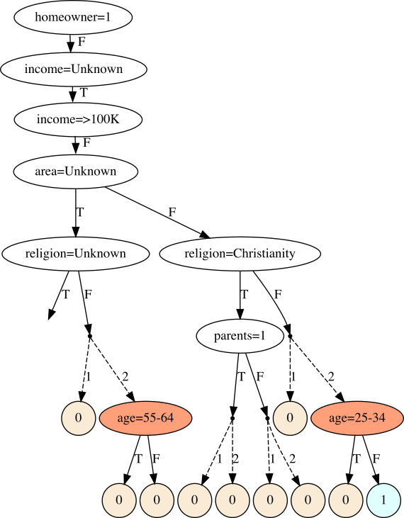
Figure 3: A subtree of the JST showing an unintended increase in predicted conversions after bias mitigation for a cohort of the already over-predicted group of non-homeowners.

6 CONCLUSION

We addressed the problem of interpretable model differencing, localizing and representing differences between ML models for the same task. We proposed JST to provide a unified view of the similarities and dissimilarities between the models as well as a succinct ruleset representation. Experimental results indicate that the proposed IMD approach yields a favorable trade-off between accuracy and interpretability in predicting model differences.

The current work is limited to comparing classifiers in terms of $0$-$1$ dissimilarity. Since IMD is based on decision trees, its interpretability is limited to domains where the features are interpretable. While we have chosen to extend greedy decision tree algorithms due to ease and scalability, the resulting JSTs accordingly have no guarantees of optimality.

Future work could seek to address the above limitations. To extend the framework to regression tasks, a potential avenue is to threshold the difference function $D(M_{1}(x),M_{2}(x))$ and apply the classification framework presented herein. The problem of interpretable model differencing for images and language remains open. The constituent features for these modalities are generally not interpretable making the diff rulesets uninterpretable without additional considerations.

7 Acknowledgements

This work was partially funded by the European Union’s Horizon Europe research and innovation programme under grant agreement no. 101070568.

Interpretable Differencing of Machine Learning Models
(Supplementary Material)

Appendix A DATASETS

The datasets used for our experiments are reported in Table 4. The $\%$ of samples belonging to each class label are also listed to show the imbalance in the original datasets.

The Pima Indians Diabetes dataset is from the KEEL repository [Alcalá-Fdez et al., 2011], the FICO HELOC dataset is collected from the FICO community [FICO, 2022 Accessed: 2022-07-31], and the bank marketing and eye movements [Salojärvi et al., 2005] datasets are from OpenML [Vanschoren et al., 2013]. The other 9 tabular datasets are collected from the UCI Repository [Dua and Graff, 2017].

Table 4: Description of Datasets

Dataset	# Rows	# Cols	# Labels	% Labels
adult	41034	13	2	[74.68, 25.32]
bankm	10578	7	2	[50.0, 50.0]
banknote	1372	4	2	[55.54, 44.46]
diabetes	768	8	2	[65.1, 34.9]
magic	19020	10	2	[35.16, 64.84]
heloc	9871	23	2	[52.03, 47.97]
mushroom	8124	22	2	[48.2, 51.8]
tictactoe	958	9	2	[34.66, 65.34]
bc	569	30	2	[37.26, 62.74]
waveform	5000	40	3	[33.84, 33.06, 33.1]
eye	10936	26	3	[34.78, 38.97, 26.24]
whitewine	4898	11	7	[0.41, 3.33, 29.75, 44.88, 17.97, 3.57, 0.1]
redwine	1599	11	6	[0.63, 3.31, 42.59, 39.9, 12.45, 1.13]

Appendix B MODELS

The model abbreviations and their expanded instantiations (as coded in Scikit-Learn [Pedregosa et al., 2011]) are shown in Table 5. Empty instantiations (e.g., GaussianNB()) correspond to default parameter settings.

The test accuracies of the models are listed in Table 6.

Table 5: Details of the Models

Abbr.	Parameters
LR	LogisticRegression(random_state=1234)
KN1	KNeighborsClassifier(n_neighbors=3)
KN2	KNeighborsClassifier()
MLP1	MLPClassifier(alpha=1e-05,hidden_layer_sizes=(15,) ,random_state=1234,solver=’lbfgs’)
MLP2	MLPClassifier(hidden_layer_sizes=(100,100), random_state=1234)
DT2	DecisionTreeClassifier(max_depth=10)
DT1	DecisionTreeClassifier(max_depth=5)
GB	GradientBoostingClassifier()
RF1	RandomForestClassifier()
RF2	RandomForestClassifier(max_depth=6,random_state=1234)
GNB	GaussianNB()

Table 6: Test Accuracy (%) of Models

Datasets	LR	KN1	DT1	MLP1	MLP2	DT2	GB	RF1	KN2	RF2	GNB
adult	81.88	82.80	84.07	74.53	84.26	84.36	85.78	82.98	83.27	83.71	79.42
bankm	74.07	73.09	77.06	71.01	66.86	76.94	80.34	80.06	74.45	78.89	71.11
banknote	98.30	100.00	97.33	100.00	100.00	97.82	99.51	99.51	100.00	99.51	83.74
diabetes	77.06	71.86	74.03	71.00	68.40	69.70	80.09	75.32	72.29	76.19	75.32
magic	79.11	79.79	82.61	81.97	84.21	84.31	86.93	88.08	80.56	85.30	72.27
heloc	71.51	65.23	71.61	72.08	71.34	67.45	73.06	73.09	67.93	73.16	69.38
mushroom	99.92	100.00	99.88	100.00	100.00	100.00	100.00	100.00	100.00	99.71	96.39
tictactoe	97.92	89.58	88.89	96.88	97.57	94.10	96.53	97.92	94.10	90.97	69.44
bc	91.81	92.98	93.57	91.23	92.40	92.40	92.40	92.98	93.57	93.57	88.89
waveform	86.27	80.67	75.60	83.87	83.93	75.73	85.20	84.33	80.93	83.87	79.53
eye	44.96	47.58	51.75	45.23	44.65	56.57	61.60	66.63	47.88	57.82	43.40
whitewine	47.28	49.86	53.54	46.94	48.16	54.63	61.22	67.14	47.41	56.87	44.29
redwine	62.71	51.88	61.04	61.46	61.88	60.62	64.17	68.75	51.04	66.25	52.08

Appendix C EXAMPLE OF JST

Here we give another example of a JST (Figure 5), and also show the separately trained surrogates (Figure 4). For this example, we have picked diabetes dataset; and LR, RF1 as the model pair.

In Figure 4, the two individual surrogates are shown side-by-side (one in pink, other in orange), and a single diverging or-node is shown at the top, highlighting that they do not share any split node between them.

Figure 5 shows the Joint Surrogate Tree for the same dataset and the model pairs. As noted earlier, the JST first tries to share nodes as much as possible before diverging to two individual subtrees corresponding to the two surrogates at the or-nodes (7 here). In this process the JST also localizes the differences into those 7 or-nodes (9 diff-rules).

As an instance, in Figure 4, we note that the root nodes are $\mathrm{Plas}<133.5$ and $\mathrm{Plas}<129.5$ for the pink and orange surrogate trees respectively. The JST in Figure 5 however, chooses $\mathrm{Plas}<127.5$ as the common root node (given by equation (4)) that aligns the surrogates to share common decisions, and allows easier comparison of the models.

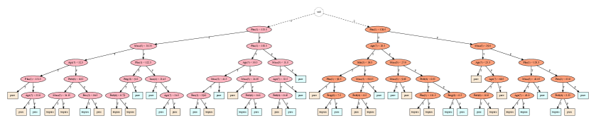
Figure 4: Separate Surrogates (shown side-by-side).

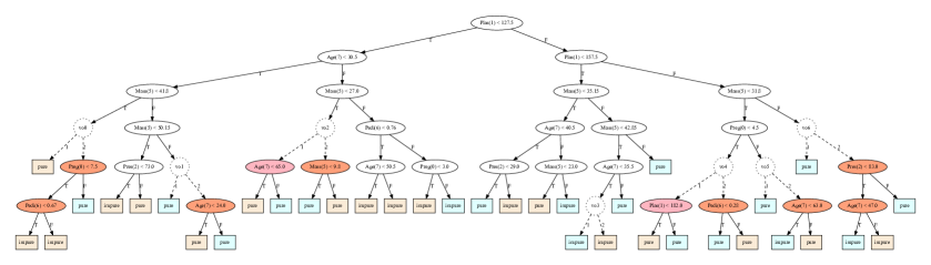
Figure 5: Joint Surrogate Tree (JST)

Appendix D REPRODUCIBILITY CHECKLIST

Code

The code is available at https://github.com/Trusted-AI/AIX360. We also provide detailed pseudocode in Appendix E.

Computing infrastructure

All the algorithms are implemented in Python 3.8, and the experiments are performed in a machine running macOS 12.4 with 2.6 GHz 6-Core Intel Core i7, and 32 GB of memory. We have used scikit-learn==1.1.1 in our environment.

ML model parameters

These are given in Table 5. As mentioned in Section 5, we did not do performance tuning of ML model parameters as our focus is on accurate model differencing and not obtaining the best performing ML models.

Appendix E ALGORITHM PSEUDOCODES

In Algorithm 1, we provide the pseudocode of the plain decision tree fitting algorithm that uses recursion. In Algorithm 2, we provide a simplified version of the JST learning algorithm that does not use or-node terminology. In Algorithm 3, the extraction procedure of diff rules from a JST is detailed, following the notations from Section 4.1.

1

Input: Samples $X$, and labels $Y$, and also the current $depth$ in the tree.

Output: A decision tree.

2

3Function dtfit ($X$, $Y$, $depth=0$)

4       if empty($X$) then

5             return none

6       end if

7      if all_same($Y$) then

8             return $Y[0]$

9       end if

10      if $depth\geq max\_depth$ then

11             return majority($Y$)

12       end if

13      $col$, $cutoff$, $ent$ = best_split($X$, $Y$)

14       return split($col$, $cutoff$, $X$, $Y$, $depth+1$)

15 end

16

17Function split($col$, $cutoff$, $X$, $Y$, $depth$)

18       $node.cond=(col<cutoff)$

19       $sl=X[:,col]<cutoff$

20       $sr=X[:,col]\geq cutoff$

21       $node.left=dtfit(X[sl],Y[sl],depth)$

22       $node.right=dtfit(X[sr],Y[sr],depth)$

23       return $node$

24 end

25

26Function best_split($X$,$Y$)

27       return $argmin,\,min_{col,val\in X[:,\,col]}$ entropy($Y$, $col$, $val$)

28 end

29

Algorithm 1 Decision Tree Algorithm

1

Input: Samples $X$, labels from $M_{1}$: $Y1$, labels from $M_{2}$: $Y2$, and also the current $depth$ in the tree.

Output: Two decision tree surrogates corresponding to $M_{1}$ and $M_{2}$.

2

3Function jointsurrogate($X$, $Y1$, $Y2$, $depth=0$)

4       if $empty(X)\lor\exists i,all\_same(Yi)\lor depth\geq max\_depth$ then

5            

6            // base conditions: if one of Y1 or Y2 is pure, diverge to give two separate trees

7            

8            return $dtfit(X1,Y1,depth)$, $dtfit(X2,Y2,depth)$

9       end if

10      $col1,cutoff1,ent1$ = $best\_split(X,Y1)$

11       $col2,cutoff2,ent2$ = $best\_split(X,Y2)$

12       $col,cutoff,jointent$ = $joint\_best\_split(X,Y1,Y2)$

13      

14      if $not\,diverge(ent1,ent2,jointent)$ then

15            

16            // shared split condition for both

17            $node1.cond=node2.cond=col<cutoff$

18             $sl=X[:,col]<cutoff$

19             $sr=X[:,col]\geq cutoff$

20             $node1.left,node2.left=jointsurrogate(X[sl],Y1[sl],Y2[sl])$

21             $node1.right,node2.right=jointsurrogate(X[sr],Y1[sr],Y2[sr])$

22             return $node1,node2$

23      else

24             // diverge to two separate subtrees (or-node)

25             // uses function from Algorithm 1

26             return $split(col1,cutoff1,X,Y1),split(col2,cutoff2,X,Y2)$

27       end if

28      

29 end

30

31Function joint_best_split($X$,$Y1$,$Y2$)

32       return $argmin,min_{col,val\in X[:,col]}$ entropy($Y1$, $col$, $val$) $+$ entropy($Y2$, $col$, $val$)

33 end

34

35Function diverge($ent1$,$ent2$, $jointent$)

36       // showing simplified divergence criterion

37       return $ent1==0\vee ent2==0$

38 end

39

Algorithm 2 Joint Surrogate Tree Learning Algorithm

1

2

Input: A node $v$ in the constructed JST. Set of constraints $path\_cond$ leading to $v$ from $root$ of JST.

Output: A list of diff-regions $dr$.

3

4Function diffreg($v$, $path\_cond$)

5      

6      if $v\in V_{d}$ then

7             // at a shared decision node

8             $ld$ = diffreg($v_{T}$, $path\_cond\wedge f(v)<t(v)$)

9             $rd$ = diffreg($v_{F}$, $path\_cond\wedge f(v)\geq t(v)$)

10             return $ld\cup rd$

11            

12      else

13             // at an or-node

14             $dr\leftarrow$ []

15             foreach $l_{1}\in leaves(v^{1})$ do

16                   foreach $l_{2}\in leaves(v^{2})$ do

17                         if $label(l_{1})\neq label(l_{2})$ then

18                               $c$ = $path\_cond\wedge pc(l_{1})\wedge pc(l_{2})$

19                               if $non\_empty(c)$ then

20                                     $dr.add(c)$

21                               end if

22                              

23                         end if

24                        

25                   end foreach

26                  

27             end foreach

28            return $dr$

29            

30       end if

31      

32 end

diffreg($JST.root$, $True$)

Algorithm 3 Diff-Regions from JST

Appendix F ADDITIONAL EXPERIMENTAL RESULTS

F.1 Fidelity Comparison

We also investigate if jointly training surrogates affects the fidelity (fraction of samples for which the surrogate predictions match with the original model’s prediction for a set of instances) of surrogates to the original models. We compute fidelity of the surrogates, $\hat{M}_{1}$ and $\hat{M}_{2}$ (corresponding to $M_{1}$ and $M_{2}$), on the held-out $\mathcal{D}_{\mathrm{test}}$. It can be seen in Table 7 that the corresponding fidelity values are very close to each other.

Conclusion

This indicates that the proposed method of jointly approximating two similar models via JSTs, achieves a way to incorporate knowledge from both models (by preferring shared nodes) without harming the individual surrogates’ faithfulness to their respective models.

Table 7: Fidelity (%) values for surrogate $\hat{M}_{i}$ are comparable for separate and joint training procedures.

		Separate		Joint
Dataset	$M_{1}$ vs. $M_{2}$	$\hat{M}_{1}$	$\hat{M}_{2}$	$\hat{M}_{1}$	$\hat{M}_{2}$
adult	max MLP1-GB	99.996	96.920	99.976	96.920
	min MLP2-DT2	91.956	98.300	91.896	98.162
bankm	max MLP2-GB	88.766	92.174	88.670	91.708
	min MLP1-GNB	90.328	95.432	89.140	93.868
banknote	max KN1-GNB	98.056	98.204	98.396	97.620
	min LR-DT1	98.156	97.864	97.526	97.864
bc	max DT1-GNB	94.270	96.610	93.216	96.142
	min KN2-RF2	95.322	93.450	92.982	93.686
diabetes	max MLP2-GB	79.828	84.416	79.222	83.984
	min RF1-GNB	80.866	86.668	77.316	87.878
eye	max RF1-GNB	56.178	86.912	48.962	86.010
	min LR-MLP1	78.982	79.038	76.282	76.974
heloc	max KN1-RF2	75.022	93.592	75.416	93.396
	min GB-RF1	92.896	79.014	92.760	79.636
magic	max RF1-GNB	86.934	96.848	86.156	96.540
	min MLP2-DT2	91.376	91.494	90.422	90.754
mushroom	max KN1-GNB	99.984	98.844	100.000	98.426
	min RF2-GNB	99.952	98.844	99.952	98.198
redwine	max RF1-KN2	63.042	62.292	63.918	62.626
	min KN1-GNB	55.998	79.582	53.498	76.918
tictactoe	max LR-GNB	89.652	91.736	90.554	93.818
	min DT2-KN2	90.970	88.544	92.152	89.098
waveform	max LR-DT1	80.334	97.774	81.600	98.252
	min MLP1-RF2	77.986	83.918	78.746	84.480
whitewine	max RF1-GNB	59.838	80.842	58.490	78.736
	min LR-KN2	90.272	55.658	89.360	53.526

F.2 Effect of Maximum Depth

In the main paper, we have set the maximum depth hyper-parameter to 6 for separate surrogates, IMD and Direct DT. That choice was made to achieve a favourable trade-off between accuracy and interpretability, and also for ease of inspection of the resulting trees as the maximum decision path length we had to look at was limited to 6.

Now we study how varying the maximum depth of the trees in the methods affects the quality (F1-score) and interpretability (no. of rules) of the resulting diff ruleset. We have varied the maximum depth from 3 to 10, and plotted the F1-score in Figure 6, and # rules in Figure 7, and elaborate on some observable trends below.

Looking at Figure 6, we observe the trend that separate surrogates achieves the highest F1 scores, followed by IMD, and then Direct DT, for most (19 out of 26) benchmarks. Typically, we also see rising values of F1 with increasing max. depth.

Interestingly, for benchmarks where the fraction of diff samples was high (e.g., eye max ($0.56$), redwine min ($0.52$), whitewine max ($0.53$)), Direct DT mostly outperformed surrogate based approaches, but on increasing depth they did catch up. On the other hand, when the fraction of diff samples were low (e.g., tictactoe min ($0.06$), heloc max ($0.23$), bankm max ($0.26$), magic min ($0.11$)) Direct DT gave close to 0 precision and recall initially, whereas both IMD and separate surrogate methods identified regions of differences.

Conclusion

The above observation also highlights that direct approaches treat difference modelling as an imbalanced classification problem only, and have the same drawbacks. Also see below (Appendix F.4) for a qualitative comparison.

In Figure 7, we observe that for separate surrogates the number of rules values are orders of magnitude higher than both IMD and Direct DT, and rises quickly (or saturates for smaller datasets, eg. banknote and bc) on increasing the maximum depth. Here, we observe that for most benchmarks, F1 values of IMD at maximum depth of 10 is very close to that of separate surrogates, but the # rules gap between them is very large, affirming the compactness of representation of JSTs.

Figure 6: Effect of varying maximum depth on F1-scores for Separate Surrogates (green), IMD (orange) and Direct DT (blue). Each plot in the figure corresponds to a dataset and a model pair, as written on the title. The vertical bars around each point indicate the standard deviation over the 5 runs. Typically, we observe the trend separate surrogates on top, IMD in the middle, and Direct DT on the bottom. The values corresponding to max. depth = $6$ are reported in main paper.

Figure 7: Interpretability (number of rules in the diff ruleset) for Separate Surrogates (green), IMD (orange) and Direct DT (blue) on varying maximum depth. Each plot in the figure corresponds to a dataset and a model pair, as written on the title. The vertical bars around each point indicate the standard deviation over the 5 runs. As seen earlier, no. of rules for separate surrogates rises quickly with depth, whereas for IMD and Direct DT it is almost always below 50. The values corresponding to max. depth = $6$ are reported in main paper.

F.3 ACCURACY-INTERPRETABILITY TRADE-OFF FOR INTERPRETABLE BASELINES

Here we compare the trade-off between F1 score and # rules for interpretable or rule-based difference prediction baselines, namely, Direct DT, separate surrogates, and the proposed method IMD. We show the trade-off plots for different dataset and model pair combinations in Figure 8. These plots are generated by plotting the F1-scores against # rules, that were obtained on varying the maximum depth hyper-parameter in the last experiment (Appendix F.2). Note that we only connect pareto-efficient points, i.e., those not dominated by points with both higher F1 score and lower # rules, with line segments for better visualization. We also plot the rules axis in log scale due to the wide range of # rules in the separate approach.

Looking at the plots, we see that Direct DT and IMD almost always achieve better trade-off than Separate. On 20 out of the 26 cases shown in Figure 8, the curves for Separate (in green) stay below (or much to the right) of those for Direct DT or IMD (in orange or blue). Also, often the green curves extend beyond $10^{3}$ rules highlighting its massive complexity.

The trade-offs for Direct DT and IMD are however more competitive, and IMD curve (in orange) is better or is as good as Direct DT for 14 out of the 26 cases. To differentiate betweeen them further, below we have done a qualitative study (Appendix F.4), and also tabulate an extended summary statistics for 10 pairs of models per dataset (Appendix F.5).

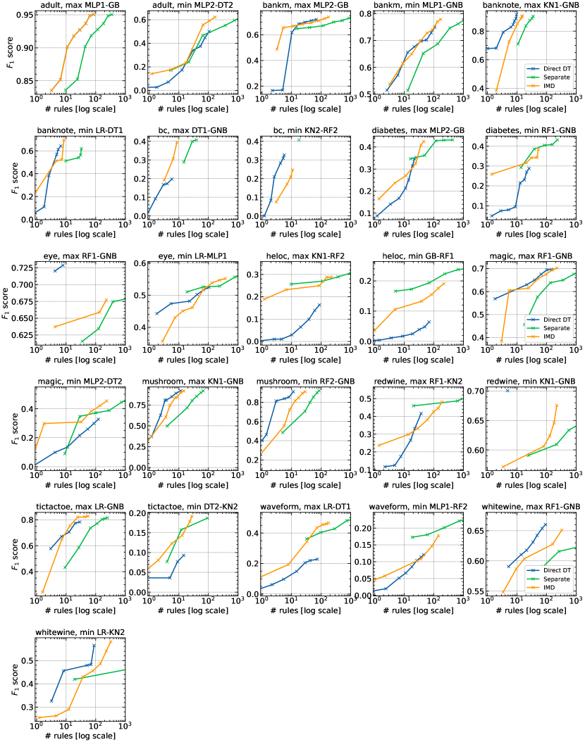
Figure 8: Trade-off between F1-score and # rules (in log scale, trimmed after $10^{3}$) for interpretable baselines. Pareto efficient points are connected by line segments and shown in the figure. For some dataset and model pairs (e.g., whitewine, max RF1-GNB), the curve for separate surrogates approach extends beyond the $10^{3}$ mark.

F.4 QUALITATIVE COMPARISON OF DIRECT DT & IMD

Next we discuss the differences between Direct DT and our proposed method IMD. In the main paper, we noted that the design of JST helps to localize the model differences in the context of overall decision logic of the models (penultimate paragraph in Section 1, also in Figure 2). Here we demonstrate that the JST’s internal decision logic (in terms of the features used) is indeed closer to that of the models, while Direct DT’s is not.

We utilise feature importance scores in decision trees (defined as the total impurity decrease brought in by a feature) to understand the top 5 most important features in Direct DT and JST. We also choose decision trees as the original two models under comparison, i.e., DT1 and DT2, for each dataset. In Figures 9, 10, and 11, we show for one dataset in each row, the top 5 features used by the models DT1 and DT2 (first two columns), Direct DT differencing (third column), and finally for the JST (the first step for IMD) built on them.

A general observation across all such rows is that the feature importance scores for JST tend to be closer to the models. As an example, for the 4-feature banknote dataset, we see both DT1 and DT2 weigh the features variance, skewness, curtosis, and entropy (in that order), which is same as JST but different from how Direct DT places them: variance, entropy, curtosis, and skewness. It is also interesting to note that while the feature skewness is rated second in the list by the models and JST, Direct DT does not use it at all (indicated by the 0 value).

We also observe that in some cases, the feature with the highest importance value in models is also placed at the top by JST, while it does not appear in the top 5 features for Direct DT. The features odor=n for mushroom dataset (3rd row in Figure 10), and mean concave points for bc dataset (1st row in Figure 11) are two such examples.

Conclusion

The above observations demonstrate that JSTs (and thus IMD) indeed faithfully capture the decision making process of the original models before localizing the differences, while Direct DT focuses solely on identifying the differences without placing them in the context of the models.

Figure 9: Feature importances for decision tree models (M1 and M2), Direct DT, and IMD (JST) for adult, bankm, banknote, and diabetes datasets (each row corresponds to a single dataset.) The importances for JST are much closer to that of the models, demonstrating their decision logics are similar.

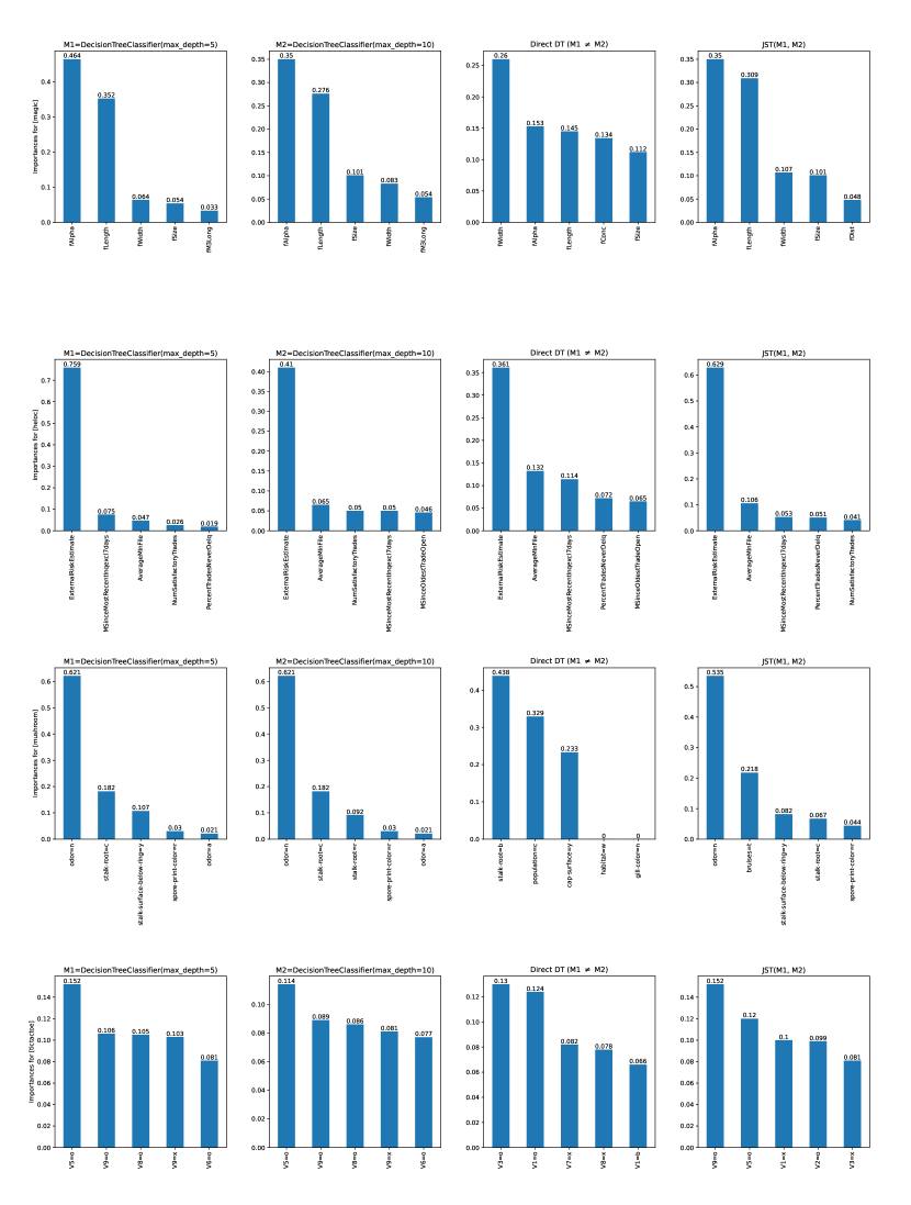
Figure 10: Feature importances for decision tree models (M1 and M2), Direct DT, and IMD (JST) for magic, heloc, mushroom, and tictactoe datasets.

Figure 11: Feature importances for decision tree models (M1 and M2), Direct DT, and IMD (JST) for bc, waveform, eye, whitewine, and redwine datasets.

F.5 Comparison of all baselines on More Benchmarks

In Section 5.2, we compared IMD against separate surrogates, Direct DT, Direct GB and BRCG Diff. on the basis of the quality of prediction of the true dissimilarity $D$ (F1 scores) for only 2 model pairs per dataset. Here we choose 10 model pairs per dataset (sorted in decreasing order of accuracy gaps), and repeat the same experiment to empirically verify the trend amongst the 5 algorithms for difference modelling. To include BRCG Diff., we compare all of them on the 9 binary classification datasets and show the summary in Table 8. In total, we have 90 dataset and model pair combinations.

We show the no. of times IMD achieved better F1 score than the other algorithms (# greater), the average % change in F1 score on going from IMD to the other algorithms, and $p-$values obtained from Wilcoxon’s signed rank test. We note a caveat in this analysis that even though the model pairs for different datasets are independent; however, for a given dataset, if the same model appears in multiple model pairs, they are not truly independent. So the $p-$values may be overstated.

We also performed Friedman’s test which confirmed significant difference amongst the algorithms with $p$- value $10^{-23}$. The mean ranks found are $3.23$, $2.16$, $3.78$, $2.1$, $3.73$ for IMD, Separate, Direct DT, Direct GB, and BRCG Diff. respectively.

Conclusion

This analysis validates that the proposed IMD approach is close to the accuracy of much more complex diff models (Separate and Direct GB), while significantly more accurate than interpretable baselines (Direct DT and BRCG Diff.).

Table 8: Summary statistics of comparisons on more benchmarks. All observed differences are significant with respect to the Holm-corrected thresholds $0.0125$, $0.017$, $0.025$, $0.05$.

	IMD vs.
Statistic	Separate	Direct DT	Direct GB	BRCG Diff.
# IMD has greater F1	$15/90$	$62/90$	$28/90$	$52/90$
% change from IMD	$19.67\%$	$-14.38\%$	$0.43\%$	$-13.49\%$
Wilcoxon’s $p$-value	$3.06e-11$	$2.60e-06$	$0.00028$	$5.09e-06$

F.6 Further results for Refinement

In this section, we show the effect of refinement at a general height $h$, with 1 and 2 iterations of selective refinement, for $h=3\,,4\,$ and $5$.

In Figure 12, we compare the precision values of $\textrm{IMD}_{h}$, $\textrm{IMD}_{h+1}$ (with 1 step refinement from height $h$) and $\textrm{IMD}_{h+1}$ (without refinement). As can be seen in the bar plots, the middle green bar corresponding to $\textrm{IMD}_{h+1}$ (with 1 level refinement from height $h$) achieves higher precision than both the IMD versions at height $h$, and $h+1$ without refinement.

We see similar trends for 2 steps of refinement in Figure 13 for $\textrm{IMD}_{h}$, $\textrm{IMD}_{h+2}$ (with 2 step refinement from height $h$) and $\textrm{IMD}_{h+2}$ (without refinement).

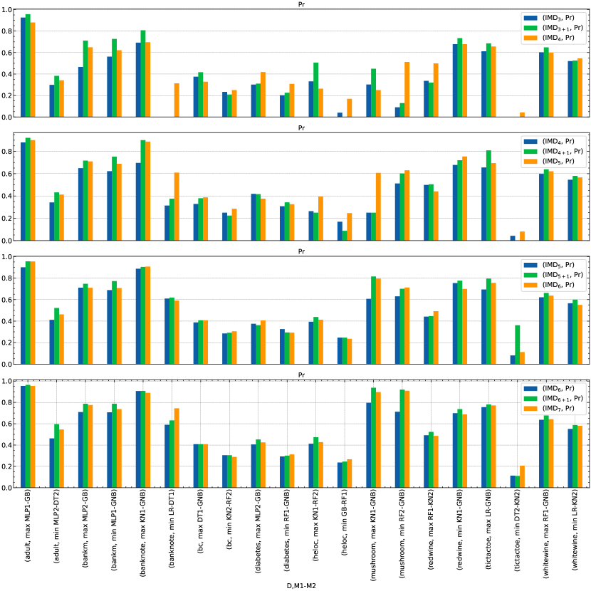
Figure 12: Precision values for $\textrm{IMD}_{h}$, $\textrm{IMD}_{h+1}$ (1 step refinement) and $\textrm{IMD}_{h+1}$ (without ref.). Each group of 3 bars (blue, green and orange) in the plot corresponds to the three methods for a dataset and model pair. The trend is, the middle green bar is higher than both its left and right bars, for most benchmarks.

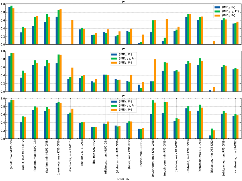
Figure 13: Precision values for $\textrm{IMD}_{h}$, $\textrm{IMD}_{h+2}$ (2 step refinement) and $\textrm{IMD}_{h+2}$ (without ref.). Each group of 3 bars (blue, green and orange) in the plot corresponds to the three methods for a dataset and model pair. The trend is, the middle green bar is higher than both its left and right bars, for most benchmarks.

F.7 Effect of the parameter $\alpha$

In the main paper, we have used the simplified divergence criterion (6) instead of (5) which was parameterized by $\alpha$. In this experiment, we study the trend of F1 scores and # rules against $\alpha$ (ranging from $0$ to $1$), with a fixed max_depth of 6.

We emphasize again that the end point $\alpha=1.0$ corresponds to separate surrogate approach, and $\alpha$ close to 0 would encourage more and more sharing of nodes.

In Figures 14 and  15, we show this trend for each dataset, and max and min gap model pairs as used earlier (Section 5.1).

Almost in all the cases, we observe sharp increase when $\alpha$ gets close to 1 i.e., the surrogates diverge away from each other. The figures in y-axis also match with prior results for separate surrogates and IMD.

Conclusion

The algorithm is sensitive to $\alpha$ close to $1$ and quickly makes a transition from conjoined trees to completely separate trees. But close to zero (typically less than $0.5$ as seen from the plots), the metrics are not sensitive to alpha.

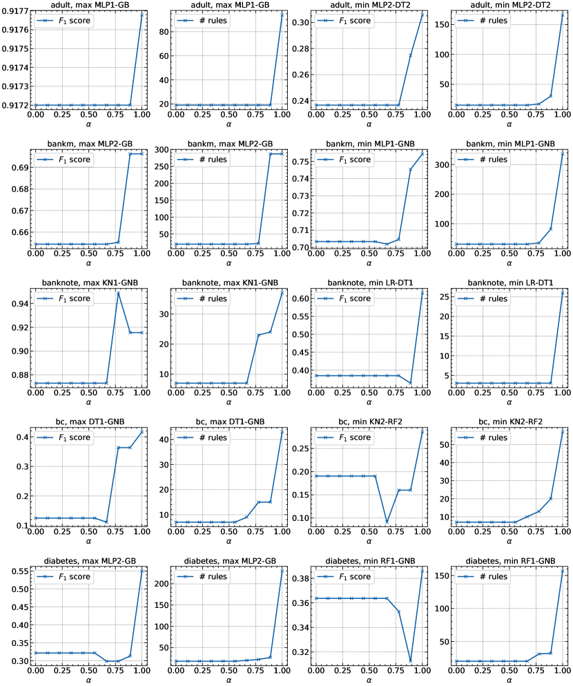
Figure 14: Effect of $\alpha$ on metrics for IMD. The algorithm is sensitive to $\alpha$ close to $1$ and quickly makes a transition from conjoined trees to completely separate trees.

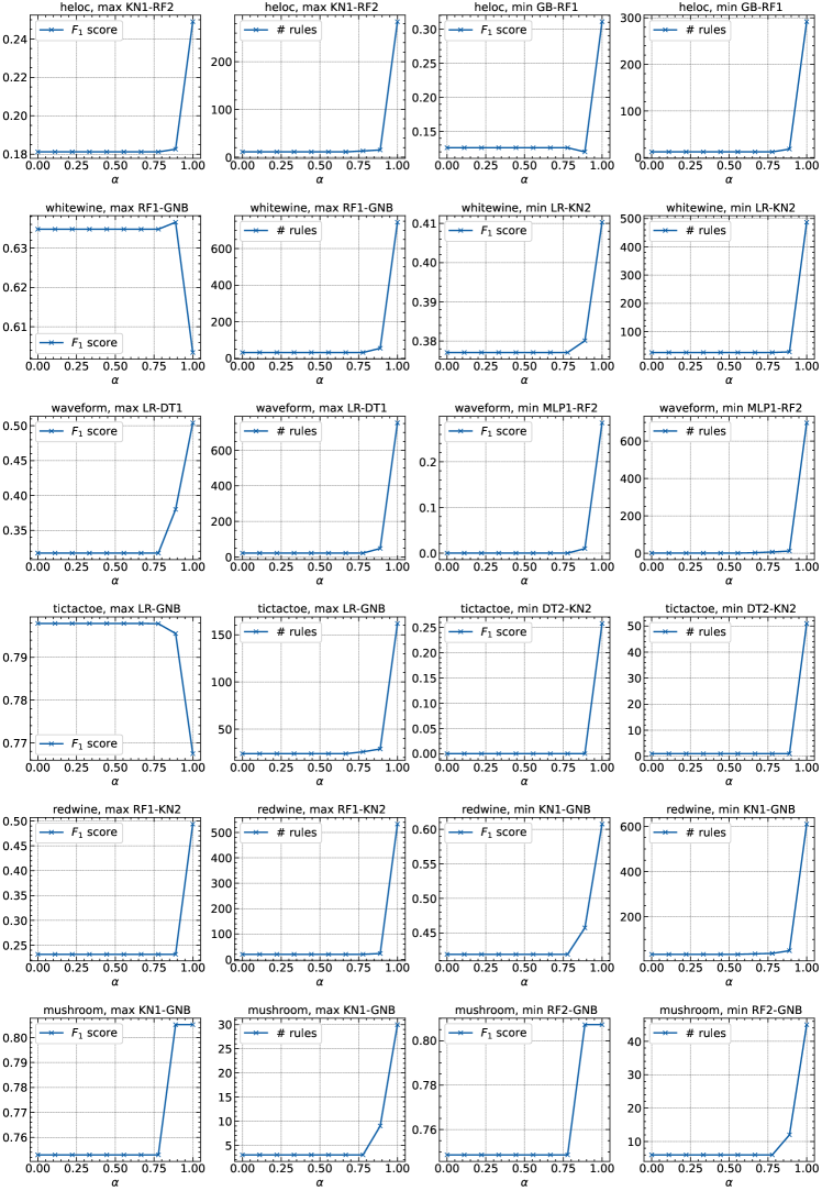
Figure 15: Effect of $\alpha$ on metrics for IMD. The algorithm is sensitive to $\alpha$ close to $1$ and quickly makes a transition from conjoined trees to completely separate trees.

F.8 Perturbation/change detection experiment

In this experiment, we artificially induce a change in the dataset (following  Nair et al. [2021]) and see if our method faithfully recovers it.

Set up

For each dataset, on the available training data with ground truth labels we first fit a model, and call it the original model. Then, we design a rule $r$, flip labels of all instances in the training data satisfying the rule with some probability $p$, and fit a revised model with the same parameters as used in the original model. We then subject these two models — original and revised — to model differencing (using proposed IMD method and separate surrogates) and verify if the extracted diff-rules recover the change inducing rule $r$.

For each dataset, and (original, revised) model combination, we vary the perturbation probability $p\in\{0.5,0.6,\dots,1.0\}$, and find the diff-rule having maximum similarity with the perturbing rule $r$ (using statistical and semantic rule similarity measures  [Nair et al., 2021]). We consider the diff-rule to have recovered the perturbation if the similarity is greater than a threshold value ($\geq 0.3$ in the experiments). Note that this is a stricter definition of recovery than just covering the support of $r$, since covering may be achieved jointly by multiple diff rules with none of them having high similarity to on their own. Also, even when we perturb the data with a single rule $r$ with some probability $p$, we observed that in the retrieved diff-ruleset, often there are multiple diff-rules that overlap (or have statistical or semantic similarity as mentioned above) with $r$.

We have experimented with 8 binary classification datasets (for simplicity in flipping class labels), 4 model classes (LR, DT2, RF1, GB) and for 5 random rules for each perturbation probability. We have also repeated the experiment for two methods of model differencing: our IMD method and separate surrogates approach (both with max_depth=6, as used in prior experiments).

We show the averaged plots in Figure 16.

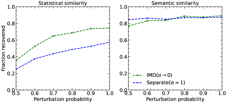
Figure 16: Both baselines are able to recover the perturbation (rule) with high similarity scores.

Conclusion

We see for both methods the recovery rate increases with perturbation probability, for both statistical and semantic similarity measures. Interestingly, IMD does better in recovering the rule than separate, because separate surrogates approach tends to generate many (and more granular) regions in the feature space to cover a larger region, whereas IMD is constrained by difference localization.

This also highlights that the differences are reliably identified by IMD in its current configuration.

Appendix G ADDITIONAL DETAILS ON CASE STUDY

In several domains involving people, machine learning models may systematically advantage certain cohorts and lead to unfair outcomes. This may be due to biases in the training data, mechanisms of data labeling and collection, or other factors. Several bias mitigation methods have been proposed to update models to correct for such biases. Our differencing method can be used to find differences in models before and after mitigation, to ensure that there were no knock-on effects of the change.

Our example is from the advertising industry where targeted ads are personalized based on user profiles. Companies through ad campaigns want to reach potential customers and use machine learning models to predict who they might be. But what models predict and actual conversions, i.e. when some one interacts with an ad, can be very different and biased. This is a poor outcome for companies who are not reaching the right audience, and for customers who are incorrectly targeted.

Using synthetic data generated from an actual ad campaign, we train a model, detect (using Multi-dimensional subset scan (MDSS) Zhang and Neill [2016]). For discovered privileged groups we measure bias using Disparate Impact Ratio, which is the likelihood of positive outcomes for unprivileged groups by positive outcomes for privileged group. A ratio of close to 1 indicates parity between two groups, while values away from 1 imply advantage to one of the groups.

In our case, MDSS reported a privileged group of non-homeowners, where predicted conversions were considerably higher than ground truth. Using this as the privileged group, the disparate impact ratio was found to be $0.48$, indicated favored status for this cohort. The test balanced accuracy of this base model is $0.5723$.

To remedy bias, we apply a mitigation using Reject Option Classification [Kamiran et al., 2012], a post-processing technique that gives favorable outcomes to unprivileged groups and unfavorable outcomes to privileged groups in a confidence band around the decision boundary with the highest uncertainty . After mitigation the disparate impact ratio improves to $1.1$ indicating better parity between groups with the test balanced accuracy of $0.568$, i.e. a negligible drop in predictive accuracy.

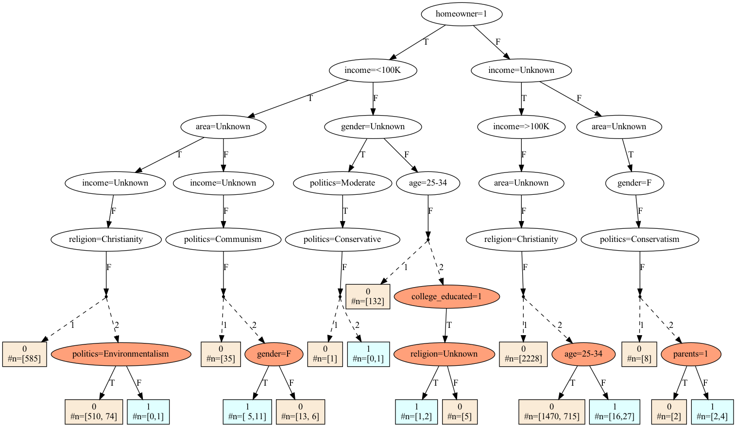
Figure 17: Joint Surrogate Tree for models before and after bias mitigation using Reject Option Classification. Parts of the tree where the outcome labels for both models are the same are hidden.

Appendix H ADDITIONAL TABLES

We have provided the complete versions of tables presented in the main paper with all the missing metrics, and standard deviations over 5 runs here.

Table 9: Full table for Separate Surrogate vs. IMD technique with added number of predicates (#p) column, and standard deviation values over 5 runs. We removed the model pairs column (available in Table 13) for brevity.

	Separate Surrogates				IMD
Dataset	Pr	Re	#r	#p	Pr	Re	#r	#p
adult	0.96 $\pm$ 0.00	0.88 $\pm$ 0.00	70.0 $\pm$ 17.77	69.2 $\pm$ 2.99	0.96 $\pm$ 0.00	0.88 $\pm$ 0.00	18.0 $\pm$ 1.26	48.4 $\pm$ 3.01
	0.45 $\pm$ 0.02	0.29 $\pm$ 0.13	155.4 $\pm$ 7.74	127.8 $\pm$ 7.7	0.46 $\pm$ 0.02	0.16 $\pm$ 0.01	17.4 $\pm$ 1.96	49.2 $\pm$ 5.08
bankm	0.66 $\pm$ 0.01	0.75 $\pm$ 0.01	263.6 $\pm$ 20.03	172.0 $\pm$ 9.38	0.70 $\pm$ 0.04	0.67 $\pm$ 0.02	23.0 $\pm$ 2.76	66.8 $\pm$ 6.14
	0.74 $\pm$ 0.02	0.75 $\pm$ 0.02	345.0 $\pm$ 7.16	177.0 $\pm$ 3.22	0.71 $\pm$ 0.01	0.69 $\pm$ 0.01	34.4 $\pm$ 1.85	83.2 $\pm$ 6.05
banknote	0.88 $\pm$ 0.02	0.89 $\pm$ 0.05	32.2 $\pm$ 5.38	48.2 $\pm$ 5.91	0.90 $\pm$ 0.04	0.88 $\pm$ 0.04	13.4 $\pm$ 2.33	37.4 $\pm$ 5.39
	0.53 $\pm$ 0.06	0.60 $\pm$ 0.04	30.8 $\pm$ 8.95	52.0 $\pm$ 7.4	0.64 $\pm$ 0.14	0.47 $\pm$ 0.21	7.2 $\pm$ 2.71	25.0 $\pm$ 6.51
bc	0.38 $\pm$ 0.08	0.46 $\pm$ 0.09	39.2 $\pm$ 7.57	34.0 $\pm$ 2.83	0.44 $\pm$ 0.16	0.40 $\pm$ 0.17	9.6 $\pm$ 1.36	27.0 $\pm$ 2.0
	0.37 $\pm$ 0.10	0.38 $\pm$ 0.11	49.0 $\pm$ 7.77	38.8 $\pm$ 2.4	0.30 $\pm$ 0.05	0.24 $\pm$ 0.15	10.8 $\pm$ 1.6	29.4 $\pm$ 2.94
diabetes	0.42 $\pm$ 0.09	0.45 $\pm$ 0.06	215.8 $\pm$ 36.22	131.4 $\pm$ 7.53	0.40 $\pm$ 0.03	0.28 $\pm$ 0.07	24.2 $\pm$ 3.37	70.6 $\pm$ 7.34
	0.39 $\pm$ 0.06	0.43 $\pm$ 0.03	156.0 $\pm$ 29.35	112.2 $\pm$ 8.18	0.31 $\pm$ 0.08	0.34 $\pm$ 0.13	20.8 $\pm$ 2.04	56.6 $\pm$ 2.58
eye	0.65 $\pm$ 0.02	0.66 $\pm$ 0.08	1054.0 $\pm$ 57.48	175.6 $\pm$ 7.42	0.60 $\pm$ 0.04	0.71 $\pm$ 0.18	36.2 $\pm$ 2.4	86.4 $\pm$ 5.2
	0.59 $\pm$ 0.01	0.53 $\pm$ 0.02	781.6 $\pm$ 32.22	227.2 $\pm$ 6.27	0.57 $\pm$ 0.02	0.39 $\pm$ 0.05	28.4 $\pm$ 1.36	76.6 $\pm$ 1.74
heloc	0.40 $\pm$ 0.03	0.23 $\pm$ 0.04	373.0 $\pm$ 58.53	200.0 $\pm$ 4.56	0.40 $\pm$ 0.05	0.13 $\pm$ 0.05	15.8 $\pm$ 3.87	53.8 $\pm$ 8.93
	0.30 $\pm$ 0.02	0.19 $\pm$ 0.08	234.4 $\pm$ 45.63	186.8 $\pm$ 4.53	0.25 $\pm$ 0.04	0.06 $\pm$ 0.02	14.6 $\pm$ 1.2	47.2 $\pm$ 4.17
magic	0.75 $\pm$ 0.02	0.58 $\pm$ 0.05	362.8 $\pm$ 29.31	179.2 $\pm$ 5.78	0.75 $\pm$ 0.02	0.52 $\pm$ 0.04	25.0 $\pm$ 1.1	71.0 $\pm$ 3.58
	0.43 $\pm$ 0.04	0.36 $\pm$ 0.02	282.6 $\pm$ 9.39	217.4 $\pm$ 2.33	0.42 $\pm$ 0.05	0.17 $\pm$ 0.04	11.0 $\pm$ 1.1	41.8 $\pm$ 3.97
mushroom	0.94 $\pm$ 0.02	0.70 $\pm$ 0.02	28.0 $\pm$ 4.86	30.6 $\pm$ 1.5	0.81 $\pm$ 0.08	0.70 $\pm$ 0.03	5.0 $\pm$ 0.0	16.0 $\pm$ 0.63
	0.93 $\pm$ 0.03	0.70 $\pm$ 0.02	42.0 $\pm$ 1.9	38.6 $\pm$ 1.5	0.74 $\pm$ 0.07	0.71 $\pm$ 0.02	8.6 $\pm$ 1.5	23.2 $\pm$ 1.72
redwine	0.46 $\pm$ 0.03	0.52 $\pm$ 0.02	627.8 $\pm$ 64.99	189.8 $\pm$ 6.52	0.52 $\pm$ 0.06	0.25 $\pm$ 0.05	29.0 $\pm$ 1.41	78.2 $\pm$ 3.87
	0.70 $\pm$ 0.04	0.59 $\pm$ 0.07	563.6 $\pm$ 89.88	175.0 $\pm$ 12.85	0.69 $\pm$ 0.05	0.47 $\pm$ 0.10	40.4 $\pm$ 4.5	93.8 $\pm$ 5.71
tictactoe	0.76 $\pm$ 0.03	0.78 $\pm$ 0.04	109.6 $\pm$ 26.7	42.4 $\pm$ 1.5	0.76 $\pm$ 0.02	0.89 $\pm$ 0.05	24.4 $\pm$ 3.01	35.0 $\pm$ 1.41
	0.10 $\pm$ 0.08	0.15 $\pm$ 0.09	54.0 $\pm$ 33.7	38.8 $\pm$ 2.64	0.16 $\pm$ 0.14	0.11 $\pm$ 0.09	5.8 $\pm$ 2.4	21.2 $\pm$ 6.49
waveform	0.45 $\pm$ 0.04	0.52 $\pm$ 0.02	746.0 $\pm$ 43.74	199.2 $\pm$ 0.98	0.49 $\pm$ 0.02	0.27 $\pm$ 0.04	33.2 $\pm$ 7.73	95.8 $\pm$ 18.73
	0.17 $\pm$ 0.04	0.32 $\pm$ 0.03	725.0 $\pm$ 91.1	237.2 $\pm$ 7.52	0.10 $\pm$ 0.05	0.02 $\pm$ 0.01	9.0 $\pm$ 3.52	33.6 $\pm$ 11.71
whitewine	0.64 $\pm$ 0.02	0.59 $\pm$ 0.03	847.2 $\pm$ 113.12	219.2 $\pm$ 7.0	0.63 $\pm$ 0.01	0.56 $\pm$ 0.08	42.6 $\pm$ 4.27	99.6 $\pm$ 6.71
	0.56 $\pm$ 0.03	0.33 $\pm$ 0.02	580.0 $\pm$ 63.9	201.2 $\pm$ 6.11	0.55 $\pm$ 0.02	0.35 $\pm$ 0.04	36.6 $\pm$ 4.67	92.0 $\pm$ 6.54

Table 10: Comparison of F1-scores with standard deviation over 5 runs. Means are already reported in main paper Table 2.

		Sep.	Direct	Direct	BRCG
Dataset	IMD	Surr.	DT	GB	Diff.
adult	0.92 $\pm$ 0.00	0.92 $\pm$ 0.00	0.92 $\pm$ 0.00	0.98 $\pm$ 0.00	0.33 $\pm$ 0.01
	0.23 $\pm$ 0.01	0.34 $\pm$ 0.09	0.17 $\pm$ 0.11	0.61 $\pm$ 0.01	0.31 $\pm$ 0.01
bankm	0.68 $\pm$ 0.02	0.70 $\pm$ 0.00	0.69 $\pm$ 0.02	0.77 $\pm$ 0.01	0.41 $\pm$ 0.01
	0.70 $\pm$ 0.00	0.75 $\pm$ 0.01	0.68 $\pm$ 0.01	0.82 $\pm$ 0.01	0.41 $\pm$ 0.00
banknote	0.89 $\pm$ 0.02	0.89 $\pm$ 0.02	0.83 $\pm$ 0.02	0.94 $\pm$ 0.01	0.27 $\pm$ 0.01
	0.52 $\pm$ 0.17	0.56 $\pm$ 0.04	0.57 $\pm$ 0.09	0.63 $\pm$ 0.06	0.06 $\pm$ 0.02
bc	0.39 $\pm$ 0.16	0.41 $\pm$ 0.06	0.17 $\pm$ 0.13	0.00 $\pm$ 0.00	0.10 $\pm$ 0.02
	0.25 $\pm$ 0.11	0.37 $\pm$ 0.11	0.28 $\pm$ 0.12	0.19 $\pm$ 0.12	0.13 $\pm$ 0.03
diabetes	0.32 $\pm$ 0.04	0.43 $\pm$ 0.08	0.21 $\pm$ 0.04	0.35 $\pm$ 0.05	0.35 $\pm$ 0.01
	0.32 $\pm$ 0.09	0.41 $\pm$ 0.04	0.09 $\pm$ 0.07	0.22 $\pm$ 0.05	0.30 $\pm$ 0.07
eye	0.63 $\pm$ 0.09	0.65 $\pm$ 0.02	0.72 $\pm$ 0.01	0.74 $\pm$ 0.01	—
	0.46 $\pm$ 0.04	0.56 $\pm$ 0.01	0.48 $\pm$ 0.03	0.59 $\pm$ 0.01	—
heloc	0.19 $\pm$ 0.05	0.29 $\pm$ 0.03	0.03 $\pm$ 0.01	0.14 $\pm$ 0.02	0.37 $\pm$ 0.02
	0.10 $\pm$ 0.02	0.22 $\pm$ 0.04	0.02 $\pm$ 0.01	0.05 $\pm$ 0.03	0.27 $\pm$ 0.07
magic	0.62 $\pm$ 0.02	0.65 $\pm$ 0.03	0.63 $\pm$ 0.04	0.78 $\pm$ 0.04	0.40 $\pm$ 0.02
	0.24 $\pm$ 0.03	0.39 $\pm$ 0.01	0.14 $\pm$ 0.03	0.27 $\pm$ 0.02	0.20 $\pm$ 0.02
mushroom	0.75 $\pm$ 0.05	0.80 $\pm$ 0.02	0.81 $\pm$ 0.05	0.97 $\pm$ 0.02	0.76 $\pm$ 0.03
	0.72 $\pm$ 0.04	0.80 $\pm$ 0.02	0.81 $\pm$ 0.02	0.97 $\pm$ 0.02	0.74 $\pm$ 0.04
redwine	0.33 $\pm$ 0.05	0.49 $\pm$ 0.02	0.17 $\pm$ 0.07	0.48 $\pm$ 0.02	—
	0.55 $\pm$ 0.07	0.63 $\pm$ 0.03	0.64 $\pm$ 0.06	0.75 $\pm$ 0.02	—
tictactoe	0.82 $\pm$ 0.02	0.77 $\pm$ 0.04	0.77 $\pm$ 0.01	0.82 $\pm$ 0.02	0.83 $\pm$ 0.04
	0.12 $\pm$ 0.10	0.12 $\pm$ 0.08	0.00 $\pm$ 0.00	0.09 $\pm$ 0.08	0.00 $\pm$ 0.00
waveform	0.34 $\pm$ 0.04	0.48 $\pm$ 0.02	0.15 $\pm$ 0.06	0.13 $\pm$ 0.03	—
	0.04 $\pm$ 0.02	0.22 $\pm$ 0.04	0.07 $\pm$ 0.01	0.06 $\pm$ 0.01	—
whitewine	0.59 $\pm$ 0.04	0.61 $\pm$ 0.01	0.62 $\pm$ 0.03	0.74 $\pm$ 0.02	—
	0.43 $\pm$ 0.04	0.41 $\pm$ 0.02	0.43 $\pm$ 0.06	0.64 $\pm$ 0.01	—

Table 11: Precision values with standard deviation over 5 runs. Means are already reported in main paper Table 3 for some of the benchmarks.

Dataset	$\text{\bf IMD}_{\text{\bf 6}}$	$\text{\bf IMD}_{\text{\bf 6+1}}$	$\text{\bf IMD}_{\text{\bf 7}}$
adult	0.96 $\pm$ 0.00	0.96 $\pm$ 0.00	0.95 $\pm$ 0.01
	0.46 $\pm$ 0.02	0.59 $\pm$ 0.03	0.53 $\pm$ 0.05
bankm	0.70 $\pm$ 0.04	0.78 $\pm$ 0.02	0.77 $\pm$ 0.03
	0.71 $\pm$ 0.01	0.79 $\pm$ 0.02	0.74 $\pm$ 0.02
banknote	0.90 $\pm$ 0.04	0.90 $\pm$ 0.03	0.89 $\pm$ 0.01
	0.64 $\pm$ 0.14	0.67 $\pm$ 0.15	0.76 $\pm$ 0.06
bc	0.44 $\pm$ 0.16	0.44 $\pm$ 0.16	0.44 $\pm$ 0.16
	0.30 $\pm$ 0.05	0.28 $\pm$ 0.08	0.26 $\pm$ 0.08
diabetes	0.40 $\pm$ 0.03	0.47 $\pm$ 0.05	0.44 $\pm$ 0.07
	0.31 $\pm$ 0.08	0.33 $\pm$ 0.11	0.34 $\pm$ 0.06
eye	0.60 $\pm$ 0.04	0.67 $\pm$ 0.01	0.62 $\pm$ 0.04
	0.57 $\pm$ 0.02	0.64 $\pm$ 0.04	0.57 $\pm$ 0.02
heloc	0.40 $\pm$ 0.05	0.45 $\pm$ 0.06	0.42 $\pm$ 0.03
	0.25 $\pm$ 0.04	0.25 $\pm$ 0.02	0.26 $\pm$ 0.02
magic	0.75 $\pm$ 0.02	0.80 $\pm$ 0.01	0.73 $\pm$ 0.02
	0.42 $\pm$ 0.05	0.55 $\pm$ 0.05	0.46 $\pm$ 0.05
mushroom	0.81 $\pm$ 0.08	0.95 $\pm$ 0.03	0.88 $\pm$ 0.05
	0.74 $\pm$ 0.07	0.94 $\pm$ 0.04	0.89 $\pm$ 0.06
redwine	0.52 $\pm$ 0.06	0.56 $\pm$ 0.07	0.48 $\pm$ 0.03
	0.69 $\pm$ 0.05	0.73 $\pm$ 0.06	0.68 $\pm$ 0.04
tictactoe	0.76 $\pm$ 0.02	0.79 $\pm$ 0.03	0.78 $\pm$ 0.03
	0.16 $\pm$ 0.14	0.19 $\pm$ 0.19	0.18 $\pm$ 0.14
waveform	0.49 $\pm$ 0.02	0.54 $\pm$ 0.03	0.49 $\pm$ 0.01
	0.10 $\pm$ 0.05	0.14 $\pm$ 0.04	0.17 $\pm$ 0.06
whitewine	0.63 $\pm$ 0.01	0.67 $\pm$ 0.03	0.64 $\pm$ 0.01
	0.55 $\pm$ 0.02	0.59 $\pm$ 0.03	0.59 $\pm$ 0.02

Table 12: Precision, Recall and Interpretability metrics for $\textrm{IMD}_{6+1}$ and $\textrm{IMD}_{7}$. The values for $\textrm{IMD}_{6}$ are reported earlier in Table 9. As can be seen, the recall values for $\textrm{IMD}_{6+1}$ are consistently lower than both $\textrm{IMD}_{6}$ and $\textrm{IMD}_{7}$. Also, as expected, $\textrm{IMD}_{6+1}$ has lower no. of rules and no. of predicates than $\textrm{IMD}_{7}$ since it does selective splitting of nodes.

	$\text{\bf IMD}_{\text{\bf 6+1}}$				$\text{\bf IMD}_{\text{\bf 7}}$
D	Pr	Re	#r	#p	Pr	Re	#r	#p
adult	0.96 $\pm$ 0.00	0.88 $\pm$ 0.00	18.0 $\pm$ 1.26	51.8 $\pm$ 3.31	0.95 $\pm$ 0.01	0.90 $\pm$ 0.01	29.4 $\pm$ 3.98	72.0 $\pm$ 7.07
	0.59 $\pm$ 0.03	0.12 $\pm$ 0.00	22.2 $\pm$ 3.31	68.6 $\pm$ 7.26	0.53 $\pm$ 0.05	0.14 $\pm$ 0.06	36.8 $\pm$ 3.12	97.8 $\pm$ 6.21
bankm	0.78 $\pm$ 0.02	0.61 $\pm$ 0.03	26.4 $\pm$ 3.72	84.6 $\pm$ 7.55	0.77 $\pm$ 0.03	0.64 $\pm$ 0.02	45.0 $\pm$ 2.0	124.2 $\pm$ 5.91
	0.79 $\pm$ 0.02	0.62 $\pm$ 0.01	40.2 $\pm$ 4.07	108.8 $\pm$ 7.36	0.74 $\pm$ 0.02	0.71 $\pm$ 0.03	58.6 $\pm$ 2.24	143.0 $\pm$ 3.9
banknote	0.90 $\pm$ 0.03	0.89 $\pm$ 0.04	13.8 $\pm$ 2.64	38.8 $\pm$ 6.11	0.89 $\pm$ 0.01	0.91 $\pm$ 0.03	14.8 $\pm$ 1.94	42.4 $\pm$ 3.93
	0.67 $\pm$ 0.15	0.48 $\pm$ 0.21	7.8 $\pm$ 3.25	26.6 $\pm$ 7.61	0.76 $\pm$ 0.06	0.65 $\pm$ 0.09	8.4 $\pm$ 2.87	28.2 $\pm$ 6.34
bc	0.44 $\pm$ 0.16	0.40 $\pm$ 0.17	9.8 $\pm$ 1.17	27.8 $\pm$ 1.33	0.44 $\pm$ 0.16	0.40 $\pm$ 0.17	9.6 $\pm$ 1.36	27.2 $\pm$ 1.72
	0.28 $\pm$ 0.08	0.22 $\pm$ 0.16	11.4 $\pm$ 1.85	30.6 $\pm$ 3.07	0.26 $\pm$ 0.08	0.22 $\pm$ 0.16	11.0 $\pm$ 1.41	30.0 $\pm$ 2.83
diabetes	0.47 $\pm$ 0.05	0.27 $\pm$ 0.04	28.0 $\pm$ 5.66	82.6 $\pm$ 12.71	0.44 $\pm$ 0.07	0.39 $\pm$ 0.04	36.6 $\pm$ 4.13	102.6 $\pm$ 9.02
	0.33 $\pm$ 0.11	0.26 $\pm$ 0.10	23.2 $\pm$ 3.31	69.2 $\pm$ 6.4	0.34 $\pm$ 0.06	0.36 $\pm$ 0.09	30.0 $\pm$ 1.67	84.8 $\pm$ 1.72
eye	0.67 $\pm$ 0.01	0.49 $\pm$ 0.09	66.0 $\pm$ 2.0	152.4 $\pm$ 5.54	0.62 $\pm$ 0.04	0.69 $\pm$ 0.17	72.6 $\pm$ 2.8	167.6 $\pm$ 7.12
	0.64 $\pm$ 0.04	0.31 $\pm$ 0.05	43.8 $\pm$ 4.45	123.8 $\pm$ 9.74	0.57 $\pm$ 0.02	0.47 $\pm$ 0.03	66.4 $\pm$ 5.16	168.2 $\pm$ 11.3
heloc	0.45 $\pm$ 0.06	0.08 $\pm$ 0.03	20.2 $\pm$ 3.87	76.4 $\pm$ 12.19	0.42 $\pm$ 0.03	0.14 $\pm$ 0.02	39.8 $\pm$ 2.93	126.4 $\pm$ 5.16
	0.25 $\pm$ 0.02	0.04 $\pm$ 0.01	21.2 $\pm$ 3.82	73.2 $\pm$ 11.65	0.26 $\pm$ 0.02	0.10 $\pm$ 0.04	38.4 $\pm$ 3.56	116.0 $\pm$ 8.79
magic	0.80 $\pm$ 0.01	0.50 $\pm$ 0.04	28.4 $\pm$ 1.02	95.4 $\pm$ 6.65	0.73 $\pm$ 0.02	0.59 $\pm$ 0.03	50.6 $\pm$ 6.62	144.0 $\pm$ 14.79
	0.55 $\pm$ 0.05	0.13 $\pm$ 0.02	14.6 $\pm$ 2.15	59.6 $\pm$ 6.22	0.46 $\pm$ 0.05	0.24 $\pm$ 0.05	32.2 $\pm$ 4.87	110.0 $\pm$ 15.79
mushroom	0.95 $\pm$ 0.03	0.70 $\pm$ 0.03	6.0 $\pm$ 0.0	18.2 $\pm$ 0.4	0.88 $\pm$ 0.05	0.81 $\pm$ 0.07	7.6 $\pm$ 0.8	22.2 $\pm$ 2.14
	0.94 $\pm$ 0.04	0.71 $\pm$ 0.02	10.2 $\pm$ 1.94	26.4 $\pm$ 2.24	0.89 $\pm$ 0.06	0.77 $\pm$ 0.08	13.2 $\pm$ 2.23	31.0 $\pm$ 0.63
redwine	0.56 $\pm$ 0.07	0.17 $\pm$ 0.01	45.4 $\pm$ 5.08	112.0 $\pm$ 10.0	0.48 $\pm$ 0.03	0.33 $\pm$ 0.08	60.4 $\pm$ 7.17	142.8 $\pm$ 13.95
	0.73 $\pm$ 0.06	0.41 $\pm$ 0.08	66.0 $\pm$ 2.83	145.4 $\pm$ 4.72	0.68 $\pm$ 0.04	0.56 $\pm$ 0.10	80.2 $\pm$ 3.54	173.6 $\pm$ 8.21
tictactoe	0.79 $\pm$ 0.03	0.76 $\pm$ 0.05	26.8 $\pm$ 4.26	40.4 $\pm$ 0.8	0.78 $\pm$ 0.03	0.80 $\pm$ 0.06	32.6 $\pm$ 2.24	41.2 $\pm$ 1.17
	0.19 $\pm$ 0.19	0.07 $\pm$ 0.06	6.4 $\pm$ 2.87	22.4 $\pm$ 7.26	0.18 $\pm$ 0.14	0.13 $\pm$ 0.05	13.0 $\pm$ 1.26	32.6 $\pm$ 3.44
waveform	0.54 $\pm$ 0.03	0.24 $\pm$ 0.04	46.6 $\pm$ 11.76	128.4 $\pm$ 24.43	0.49 $\pm$ 0.01	0.39 $\pm$ 0.05	72.2 $\pm$ 11.03	188.2 $\pm$ 18.91
	0.14 $\pm$ 0.04	0.02 $\pm$ 0.01	13.6 $\pm$ 5.82	48.4 $\pm$ 18.64	0.17 $\pm$ 0.06	0.08 $\pm$ 0.03	36.0 $\pm$ 2.97	123.4 $\pm$ 8.64
whitewine	0.67 $\pm$ 0.03	0.45 $\pm$ 0.08	74.8 $\pm$ 8.47	169.6 $\pm$ 14.72	0.64 $\pm$ 0.01	0.54 $\pm$ 0.07	91.2 $\pm$ 11.74	200.0 $\pm$ 19.15
	0.59 $\pm$ 0.03	0.28 $\pm$ 0.05	57.2 $\pm$ 11.02	144.0 $\pm$ 16.77	0.59 $\pm$ 0.02	0.37 $\pm$ 0.04	79.8 $\pm$ 10.17	190.2 $\pm$ 16.68

Table 13: Precision & Recall values for Direct DT, Direct GB and BRCG Diff. with standard deviation over 5 runs. F1-scores are already reported in main paper Table 2.

		Direct DT		Direct GB		BRCG Diff.
Dataset	$M_{1}$ vs. $M_{2}$	Pr	Re	Pr	Re	Pr	Re
adult	max MLP1-GB	0.96 $\pm$ 0.00	0.88 $\pm$ 0.00	0.98 $\pm$ 0.00	0.97 $\pm$ 0.00	0.20 $\pm$ 0.01	1.00 $\pm$ 0.00
	min MLP2-DT2	0.61 $\pm$ 0.06	0.11 $\pm$ 0.09	0.83 $\pm$ 0.01	0.48 $\pm$ 0.01	0.22 $\pm$ 0.02	0.59 $\pm$ 0.10
bankm	max MLP2-GB	0.76 $\pm$ 0.02	0.63 $\pm$ 0.02	0.85 $\pm$ 0.02	0.70 $\pm$ 0.01	0.26 $\pm$ 0.01	1.00 $\pm$ 0.00
	min MLP1-GNB	0.67 $\pm$ 0.01	0.69 $\pm$ 0.02	0.84 $\pm$ 0.01	0.80 $\pm$ 0.02	0.26 $\pm$ 0.00	1.00 $\pm$ 0.00
banknote	max KN1-GNB	0.95 $\pm$ 0.04	0.74 $\pm$ 0.06	0.95 $\pm$ 0.02	0.92 $\pm$ 0.03	0.16 $\pm$ 0.01	1.00 $\pm$ 0.01
	min LR-DT1	0.69 $\pm$ 0.15	0.50 $\pm$ 0.09	0.80 $\pm$ 0.07	0.53 $\pm$ 0.09	0.03 $\pm$ 0.01	1.00 $\pm$ 0.00
bc	max DT1-GNB	0.20 $\pm$ 0.13	0.16 $\pm$ 0.14	0.00 $\pm$ 0.00	0.00 $\pm$ 0.00	0.05 $\pm$ 0.01	0.86 $\pm$ 0.09
	min KN2-RF2	0.40 $\pm$ 0.24	0.23 $\pm$ 0.09	0.23 $\pm$ 0.12	0.17 $\pm$ 0.13	0.07 $\pm$ 0.02	0.89 $\pm$ 0.05
diabetes	max MLP2-GB	0.43 $\pm$ 0.09	0.14 $\pm$ 0.03	0.57 $\pm$ 0.09	0.26 $\pm$ 0.03	0.22 $\pm$ 0.01	0.96 $\pm$ 0.03
	min RF1-GNB	0.27 $\pm$ 0.21	0.08 $\pm$ 0.09	0.34 $\pm$ 0.10	0.17 $\pm$ 0.04	0.18 $\pm$ 0.04	1.00 $\pm$ 0.00
eye	max RF1-GNB	0.61 $\pm$ 0.01	0.90 $\pm$ 0.01	0.68 $\pm$ 0.01	0.82 $\pm$ 0.03	—	—
	min LR-MLP1	0.62 $\pm$ 0.02	0.40 $\pm$ 0.04	0.70 $\pm$ 0.02	0.51 $\pm$ 0.01	—	—
heloc	max KN1-RF2	0.36 $\pm$ 0.08	0.02 $\pm$ 0.01	0.42 $\pm$ 0.01	0.09 $\pm$ 0.01	0.23 $\pm$ 0.01	1.00 $\pm$ 0.00
	min GB-RF1	0.16 $\pm$ 0.07	0.01 $\pm$ 0.00	0.23 $\pm$ 0.04	0.03 $\pm$ 0.02	0.16 $\pm$ 0.05	1.00 $\pm$ 0.00
magic	max RF1-GNB	0.69 $\pm$ 0.02	0.58 $\pm$ 0.07	0.85 $\pm$ 0.02	0.71 $\pm$ 0.05	0.25 $\pm$ 0.01	1.00 $\pm$ 0.00
	min MLP2-DT2	0.58 $\pm$ 0.03	0.08 $\pm$ 0.02	0.61 $\pm$ 0.03	0.17 $\pm$ 0.01	0.11 $\pm$ 0.01	1.00 $\pm$ 0.00
mushroom	max KN1-GNB	0.78 $\pm$ 0.04	0.84 $\pm$ 0.08	0.97 $\pm$ 0.02	0.96 $\pm$ 0.03	0.89 $\pm$ 0.06	0.67 $\pm$ 0.08
	min RF2-GNB	0.77 $\pm$ 0.03	0.87 $\pm$ 0.03	0.98 $\pm$ 0.02	0.95 $\pm$ 0.04	0.89 $\pm$ 0.06	0.64 $\pm$ 0.08
redwine	max RF1-KN2	0.50 $\pm$ 0.12	0.11 $\pm$ 0.06	0.60 $\pm$ 0.06	0.40 $\pm$ 0.03	—	—
	min KN1-GNB	0.65 $\pm$ 0.04	0.65 $\pm$ 0.13	0.74 $\pm$ 0.03	0.75 $\pm$ 0.03	—	—
tictactoe	max LR-GNB	0.75 $\pm$ 0.03	0.80 $\pm$ 0.05	0.81 $\pm$ 0.02	0.83 $\pm$ 0.03	0.90 $\pm$ 0.02	0.77 $\pm$ 0.07
	min DT2-KN2	0.00 $\pm$ 0.00	0.00 $\pm$ 0.00	0.23 $\pm$ 0.20	0.06 $\pm$ 0.06	0.00 $\pm$ 0.00	0.00 $\pm$ 0.00
waveform	max LR-DT1	0.31 $\pm$ 0.03	0.10 $\pm$ 0.05	0.49 $\pm$ 0.06	0.08 $\pm$ 0.02	—	—
	min MLP1-RF2	0.21 $\pm$ 0.05	0.04 $\pm$ 0.01	0.25 $\pm$ 0.07	0.03 $\pm$ 0.01	—	—
whitewine	max RF1-GNB	0.65 $\pm$ 0.03	0.60 $\pm$ 0.07	0.72 $\pm$ 0.02	0.77 $\pm$ 0.05	—	—
	min LR-KN2	0.57 $\pm$ 0.02	0.36 $\pm$ 0.09	0.69 $\pm$ 0.02	0.60 $\pm$ 0.02	—	—

Table 14: Interpretability metrics for Direct DT and BRCG Diff. with standard deviation over 5 runs.

		Direct DT		BRCG Diff.
Dataset	$M_{1}$ vs. $M_{2}$	#r	#p	#r	#p
adult	max MLP1-GB	18.2 $\pm$ 1.17	49.0 $\pm$ 2.53	2.0 $\pm$ 0.0	9.0 $\pm$ 0.71
	min MLP2-DT2	12.8 $\pm$ 0.4	45.6 $\pm$ 0.49	4.5 $\pm$ 0.5	20.0 $\pm$ 1.87
bankm	max MLP2-GB	17.4 $\pm$ 1.02	54.8 $\pm$ 3.19	22.0 $\pm$ 7.0	30.25 $\pm$ 2.28
	min MLP1-GNB	21.8 $\pm$ 1.94	60.6 $\pm$ 5.0	18.0 $\pm$ 3.0	24.5 $\pm$ 1.66
banknote	max KN1-GNB	6.2 $\pm$ 1.17	19.4 $\pm$ 3.93	19.5 $\pm$ 2.29	27.0 $\pm$ 1.22
	min LR-DT1	4.8 $\pm$ 1.33	16.4 $\pm$ 3.72	6.5 $\pm$ 1.5	13.75 $\pm$ 2.38
bc	max DT1-GNB	4.0 $\pm$ 1.1	12.8 $\pm$ 2.99	43.0 $\pm$ 6.6	31.0 $\pm$ 2.12
	min KN2-RF2	4.2 $\pm$ 0.4	13.0 $\pm$ 0.89	33.0 $\pm$ 10.25	30.25 $\pm$ 5.89
diabetes	max MLP2-GB	11.0 $\pm$ 0.63	37.2 $\pm$ 2.32	95.25 $\pm$ 16.13	69.5 $\pm$ 5.59
	min RF1-GNB	8.8 $\pm$ 3.71	29.2 $\pm$ 9.81	95.75 $\pm$ 32.86	61.75 $\pm$ 5.72
eye	max RF1-GNB	19.6 $\pm$ 2.15	52.6 $\pm$ 5.54	—	—
	min LR-MLP1	23.2 $\pm$ 2.48	67.6 $\pm$ 4.5	—	—
heloc	max KN1-RF2	10.2 $\pm$ 1.94	35.8 $\pm$ 4.92	4.5 $\pm$ 1.12	12.5 $\pm$ 3.2
	min GB-RF1	8.8 $\pm$ 3.06	34.4 $\pm$ 9.83	1.75 $\pm$ 0.43	7.0 $\pm$ 0.0
magic	max RF1-GNB	21.4 $\pm$ 0.8	65.8 $\pm$ 3.31	22.25 $\pm$ 2.05	24.25 $\pm$ 0.43
	min MLP2-DT2	11.2 $\pm$ 3.19	40.8 $\pm$ 9.26	14.25 $\pm$ 1.79	21.0 $\pm$ 3.08
mushroom	max KN1-GNB	3.4 $\pm$ 0.8	12.4 $\pm$ 2.33	32.75 $\pm$ 1.79	18.75 $\pm$ 0.43
	min RF2-GNB	3.0 $\pm$ 0.0	10.6 $\pm$ 0.49	22.75 $\pm$ 1.79	16.0 $\pm$ 0.0
redwine	max RF1-KN2	11.6 $\pm$ 2.06	34.4 $\pm$ 6.44	—	—
	min KN1-GNB	18.8 $\pm$ 1.72	51.2 $\pm$ 5.64	—	—
tictactoe	max LR-GNB	20.2 $\pm$ 2.14	34.4 $\pm$ 2.65	161.25 $\pm$ 12.19	34.5 $\pm$ 1.12
	min DT2-KN2	1.6 $\pm$ 0.8	8.4 $\pm$ 3.2	79.5 $\pm$ 2.96	30.25 $\pm$ 2.28
waveform	max LR-DT1	14.8 $\pm$ 1.33	51.0 $\pm$ 3.52	—	—
	min MLP1-RF2	11.2 $\pm$ 0.75	39.6 $\pm$ 2.15	—	—
whitewine	max RF1-GNB	21.0 $\pm$ 2.1	55.2 $\pm$ 4.53	—	—
	min LR-KN2	24.8 $\pm$ 1.94	68.8 $\pm$ 3.76	—	—

References

- Aghaei et al. [2019] Sina Aghaei, Mohammad Javad Azizi, and Phebe Vayanos. Learning optimal and fair decision trees for non-discriminative decision-making. In Proceedings of the AAAI Conference on Artificial Intelligence, volume 33, pages 1418–1426, 2019.
- Alcalá-Fdez et al. [2011] Jesús Alcalá-Fdez, Alberto Fernández, Julián Luengo, Joaquín Derrac, Salvador García, Luciano Sánchez, and Francisco Herrera. Keel data-mining software tool: data set repository, integration of algorithms and experimental analysis framework. Journal of Multiple-Valued Logic & Soft Computing, 17, 2011.
- Andriushchenko and Hein [2019] Maksym Andriushchenko and Matthias Hein. Provably robust boosted decision stumps and trees against adversarial attacks. Advances in Neural Information Processing Systems, 32, 2019.
- Ba and Caruana [2014] Jimmy Ba and Rich Caruana. Do deep nets really need to be deep? In Advances in Neural Information Processing Systems (NeurIPS), pages 2654–2662, 2014. URL http://papers.nips.cc/paper/5484-do-deep-nets-really-need-to-be-deep.pdf.
- Bansal et al. [2019] Gagan Bansal, Besmira Nushi, Ece Kamar, Walter S Lasecki, Daniel S Weld, and Eric Horvitz. Beyond accuracy: The role of mental models in human-ai team performance. In Proceedings of the AAAI Conference on Human Computation and Crowdsourcing, volume 7, pages 2–11, 2019.
- Bastani et al. [2017] Osbert Bastani, Carolyn Kim, and Hamsa Bastani. Interpretability via model extraction. In Workshop on Fairness, Accountability, and Transparency in Machine Learning (FAT/ML), 2017. URL https://arxiv.org/abs/1706.09773.
- Benavoli et al. [2016] Alessio Benavoli, Giorgio Corani, and Francesca Mangili. Should we really use post-hoc tests based on mean-ranks? Journal of Machine Learning Research, 17(5):1–10, 2016. URL http://jmlr.org/papers/v17/benavoli16a.html.
- Bu et al. [2019] Y. Bu, J. Lu, and V. V. Veeravalli. Model change detection with application to machine learning. In ICASSP 2019 - 2019 IEEE International Conference on Acoustics, Speech and Signal Processing (ICASSP), pages 5341–5346, 2019.
- Bucilă et al. [2006] Cristian Bucilă, Rich Caruana, and Alexandru Niculescu-Mizil. Model compression. In Proceedings of the 12th ACM SIGKDD International Conference on Knowledge Discovery and Data Mining (KDD), page 535–541, 2006. URL https://doi.org/10.1145/1150402.1150464.
- Chen et al. [2019] Hongge Chen, Huan Zhang, Duane Boning, and Cho-Jui Hsieh. Robust decision trees against adversarial examples. In International Conference on Machine Learning, pages 1122–1131. PMLR, 2019.
- Chouldechova and G’Sell [2017] Alexandra Chouldechova and Max G’Sell. Fairer and more accurate, but for whom? arXiv preprint arXiv:1707.00046, 2017.
- Cito et al. [2021] Jürgen Cito, Isil Dillig, Seohyun Kim, Vijayaraghavan Murali, and Satish Chandra. Explaining mispredictions of machine learning models using rule induction. In Proceedings of the 29th ACM Joint Meeting on European Software Engineering Conference and Symposium on the Foundations of Software Engineering, pages 716–727, 2021.
- Craven [1996] Mark William Craven. Extracting Comprehensible Models from Trained Neural Networks. PhD thesis, 1996. AAI9700774.
- Dash et al. [2018] Sanjeeb Dash, Oktay Gunluk, and Dennis Wei. Boolean decision rules via column generation. Advances in neural information processing systems, 31, 2018.
- Demšar [2006] Janez Demšar. Statistical comparisons of classifiers over multiple data sets. Journal of Machine Learning Research, 7(1):1–30, 2006. URL http://jmlr.org/papers/v7/demsar06a.html.
- Demšar and Bosnić [2018] Jaka Demšar and Zoran Bosnić. Detecting concept drift in data streams using model explanation. Expert Syst. Appl., 92:546–559, 2018.
- Dua and Graff [2017] Dheeru Dua and Casey Graff. UCI machine learning repository, 2017. URL http://archive.ics.uci.edu/ml.
- Duckworth et al. [2021] Christopher Duckworth, Francis P Chmiel, Dan K Burns, Zlatko D Zlatev, Neil M White, Thomas WV Daniels, Michael Kiuber, and Michael J Boniface. Using explainable machine learning to characterise data drift and detect emergent health risks for emergency department admissions during covid-19. Scientific reports, 11(1):1–10, 2021.
- FICO [2022 Accessed: 2022-07-31] FICO. Explainable Machine Learning Challenge. https://community.fico.com/s/explainable-machine-learning-challenge?tabset-158d9=3, 2022 Accessed: 2022-07-31.
- Freitas [2014] Alex A Freitas. Comprehensible classification models: a position paper. ACM SIGKDD explorations newsletter, 15(1):1–10, 2014.
- Frosst and Hinton [2017] Nicholas Frosst and Geoffrey Hinton. Distilling a neural network into a soft decision tree. In Comprehensibility and Explanation in AI and ML (CEX) Workshop, 16th International Conference of the Italian Association for Artificial Intelligence (AI*IA), 2017. URL https://arxiv.org/pdf/1711.09784.pdf.
- Geng et al. [2019] Jun Geng, Bingwen Zhang, Lauren M. Huie, and Lifeng Lai. Online change-point detection of linear regression models. IEEE Transactions on Signal Processing, 67(12):3316–3329, 2019.
- Harel et al. [2014] Maayan Harel, Koby Crammer, Ran El-Yaniv, and Shie Mannor. Concept drift detection through resampling. In Proceedings of the 31st International Conference on International Conference on Machine Learning - Volume 32, ICML’14, page II–1009–II–1017. JMLR.org, 2014.
- Hinton et al. [2015] Geoffrey Hinton, Oriol Vinyals, and Jeffrey Dean. Distilling the knowledge in a neural network. In NIPS Deep Learning and Representation Learning Workshop, 2015. URL http://arxiv.org/abs/1503.02531.
- Kamiran et al. [2012] Faisal Kamiran, Asim Karim, and Xiangliang Zhang. Decision theory for discrimination-aware classification. In 2012 IEEE 12th International Conference on Data Mining, pages 924–929. IEEE, 2012.
- Kulesza et al. [2012] Todd Kulesza, Simone Stumpf, Margaret Burnett, and Irwin Kwan. Tell me more? the effects of mental model soundness on personalizing an intelligent agent. In Proceedings of the SIGCHI Conference on Human Factors in Computing Systems, pages 1–10, 2012.
- Lakkaraju et al. [2016] Himabindu Lakkaraju, Stephen H Bach, and Jure Leskovec. Interpretable decision sets: A joint framework for description and prediction. In International Conference on Knowledge Discovery and Data Mining, pages 1675–1684, 2016.
- Letham et al. [2015] Benjamin Letham, Cynthia Rudin, Tyler H McCormick, and David Madigan. Interpretable classifiers using rules and bayesian analysis: Building a better stroke prediction model. The Annals of Applied Statistics, 9(3):1350–1371, 2015.
- Lopez-Paz et al. [2016] David Lopez-Paz, Léon Bottou, Bernhard Schölkopf, and Vladimir Vapnik. Unifying distillation and privileged information. In International Conference on Learning Representations (ICLR), 2016. URL http://leon.bottou.org/papers/lopez-paz-2016.
- Moshkovitz et al. [2021] Michal Moshkovitz, Yao-Yuan Yang, and Kamalika Chaudhuri. Connecting interpretability and robustness in decision trees through separation. In International Conference on Machine Learning, pages 7839–7849. PMLR, 2021.
- Nair et al. [2021] Rahul Nair, Massimiliano Mattetti, Elizabeth Daly, Dennis Wei, Oznur Alkan, and Yunfeng Zhang. What changed? interpretable model comparison. IJCAI, 2021.
- Pedregosa et al. [2011] Fabian Pedregosa, Gaël Varoquaux, Alexandre Gramfort, Vincent Michel, Bertrand Thirion, Olivier Grisel, Mathieu Blondel, Peter Prettenhofer, Ron Weiss, Vincent Dubourg, et al. Scikit-learn: Machine learning in python. the Journal of machine Learning research, 12:2825–2830, 2011.
- Quinlan [1986] JR Quinlan. Induction of decision trees. mach. learn. 1986.
- Salojärvi et al. [2005] Jarkko Salojärvi, Kai Puolamäki, Jaana Simola, Lauri Kovanen, Ilpo Kojo, and Samuel Kaski. Inferring relevance from eye movements: Feature extraction. In Workshop at NIPS 2005, in Whistler, BC, Canada, on December 10, 2005., page 45, 2005.
- Tan et al. [2018] Sarah Tan, Rich Caruana, Giles Hooker, and Yin Lou. Distill-and-compare: Auditing black-box models using transparent model distillation. In Proceedings of the 2018 AAAI/ACM Conference on AI, Ethics, and Society (AIES), page 303–310, 2018. URL https://doi.org/10.1145/3278721.3278725.
- Vanschoren et al. [2013] Joaquin Vanschoren, Jan N. van Rijn, Bernd Bischl, and Luis Torgo. Openml: networked science in machine learning. SIGKDD Explorations, 15(2):49–60, 2013. 10.1145/2641190.2641198. URL http://doi.acm.org/10.1145/2641190.264119.
- Zhang and Neill [2016] Zhe Zhang and Daniel B Neill. Identifying significant predictive bias in classifiers. arXiv preprint arXiv:1611.08292, 2016.