Rate-Splitting Multiple Access for Simultaneous Multi-User Communication and Multi-Target Sensing

Abstract

In this paper, we initiate the study of rate-splitting multiple access (RSMA) for a mono-static integrated sensing and communication (ISAC) system, where the dual-functional base station (BS) simultaneously communicates with multiple users and detects multiple moving targets. We aim at optimizing the ISAC waveform to jointly maximize the max-min fairness (MMF) rate of the communication users and minimize the largest eigenvalue of the Cramér-Rao bound (CRB) matrix for unbiased estimation. The CRB matrix considered in this work is general as it involves the estimation of angular direction, complex reflection coefficient, and Doppler frequency for multiple moving targets. Simulation results demonstrate that RSMA maintains a larger communication and sensing trade-off than conventional space-division multiple access (SDMA) and it is capable of detecting multiple targets with a high detection accuracy. The finding highlights the potential of RSMA as an effective and powerful strategy for interference management in the general multi-user multi-target ISAC systems.

I Introduction

Integrated sensing and communication (ISAC) has gained recognition as a promising enabling technology for 6G and beyond. The integration of these two functionalities into a unified framework is expected to unlock a wide range of new use cases and applications by elevating the overall performance, such as spectral efficiency and sensing accuracy. Additionally, in light of the conflict and resource competition between remote sensing and communication, ISAC offers two significant advantages: integration gain and coordination gain, which stem from the shared utilization of spectrum, hardware architecture, and a collaborative signal processing platform. One major challenge in ISAC lies in designing a dual-functional waveform, which is typically divided into the following three categories: sensing-centric design, communication-centric design, and joint design [1]. In this work, we dedicate to the joint design category, which has been a mainstream in ISAC.

Another challenge introduced by ISAC is the interference between communication and sensing, which occurs due to the overlapping frequency bands. Recent studies have shown that rate-splitting multiple access (RSMA), an advanced multiple access and dynamic interference management strategy, is capable to address the challenge and achieves a flexible and robust interference management between communication and sensing or among communication users[2, 3, 4, 5]. The concept of RSMA-assisted ISAC was initially explored in[2], which highlights that the common stream of RSMA serves dual purposes. It not only better manages interference between communication users, but also acts as a radar sequence to match the transmit beampattern. Further, [3] showed the advantages of RSMA-assisted ISAC in a practical scenario of partial channel state information (CSIT) and moving communication users. [4] extended RSMA-assisted ISAC from terrestrial communications to satellite communications. Additionally, [5] demonstrated that RSMA improves the trade-off between max-min fairness (MMF) rate and Cramér-Rao bound (CRB) of the single sensing target. However, all aforementioned works are limited to the study of single-target sensing. To the best of our knowledge, the performance of RSMA in multi-user multi-target ISAC has not been investigated yet.

In this work, we initiate the study of RSMA in a multi-user multi-target ISAC system. To measure the sensing performance of multiple moving targets, we derive a more general CRB radar sensing metric by involving the estimation of angular direction, complex reflection coefficient, and Doppler frequency for the targets. Simulation results demonstrate that RSMA-assisted multi-user multi-target ISAC maintains a better communication and sensing trade-off than space division multiple access (SDMA) and it detects multiple targets with a high detection accuracy.

II System Model

We consider a mono-static ISAC system assisted by RSMA, where the transmit antennas are shared by the communication users and the moving targets. The base station (BS), equipped with $N_{t}$ transmit antennas and $N_{r}$ receive antennas, simultaneously communicates with $K$ single-antenna downlink communication users and detects $M$ moving targets. The communication users and moving targets are indexed by $\mathcal{K}=\left\{1,\dots,K\right\}$ and $\mathcal{M}=\left\{1,\dots,M\right\}$, respectively.

Consider the simplest and practical 1-layer RSMA model [6], where the message $U_{k}$ intended for communication user $k$ is split into a common message $U_{c,k}$ and a private message $U_{p,k}$, respectively. All common parts are collectively encoded into a single common stream $s_{c}$, and the private parts are separately encoded into private streams $\left\{s_{p,k}\right\}_{k=1}^{K}$. Consider $N$ transmission and radar pulse blocks in one coherent processing interval (CPI) indexed by $\mathcal{N}=[1,\dots,N]$, the transmit data stream vector at each time index $n$ is $\mathbf{s}[n]=[s_{c}[n],s_{p,1}[n],\dots,s_{p,K}[n]]^{T}\in\mathbb{C}^{(K+1)\times 1}$. The streams are linearly precoded by the precoding matrix $\mathbf{W}=[\mathbf{w}_{c},\mathbf{w}_{1},\dots,\mathbf{w}_{K}]\in\mathbb{C}^{N_{t}\times(K+1)}$, which remains consistent during one CPI. The transmit signal at time index $n$ is

$$\mathbf{x}[n]=\mathbf{W}\mathbf{s}[n]=\mathbf{w}_{c}s_{c}[n]+\sum_{k\in\mathcal{K}}\mathbf{w}_{k}s_{p,k}[n],$$ (1)

where the data streams satisfy $\mathbf{s}[n]\mathbf{s}[n]^{H}=\mathbf{I}_{K+1}$, implying that the entries are independent from each other. Hence, the covariance matrix of the transmit signal can be calculated by $\mathbf{R}_{x}=\frac{1}{N}\sum_{n\in\mathcal{N}}\mathbf{x}[n]\mathbf{x}[n]^{H}=\mathbf{W}\mathbf{W}^{H}$.

The signal received at the $k$th communication user at time index $n$ is given as

$$y_{k}[n] =\mathbf{h}_{k}^{H}\mathbf{x}[n]+z_{k}[n]$$ (2)

$$=\mathbf{h}_{k}^{H}\mathbf{w}_{c}s_{c}[n]+\sum_{i\in\mathcal{K}}\mathbf{h}_{k}^{H}\mathbf{w}_{i}s_{p,i}[n]+z_{k}[n],\forall k\in\mathcal{K},$$

where $\mathbf{h}_{k}\in\mathbb{C}^{N_{t}\times 1}$ is the communication channel between the BS and user $k$. It is assumed to be perfectly known at the BS and communication users. $z_{k}[n]$ is the additive white Gaussian noise (AWGN) received at user $k$, which follows the distribution of $\mathcal{CN}(0,\sigma_{c}^{2})$.

As the transmit signal is also utilized for detecting the moving targets, the radar echo signal received at the BS at time index $n$ is defined as

$$\mathbf{y}_{s}[n]=\sum_{m\in\mathcal{M}}\alpha_{m}e^{j2\pi\mathcal{F}_{D_{m}}nT}\mathbf{b}(\theta_{m})\mathbf{a}^{T}(\theta_{m})\mathbf{x}[n]+\mathbf{z}_{s}[n],$$ (3)

where $\left\{\alpha_{m}\right\}_{m=1}^{M}$ represent the complex reflection coefficients proportional to the targets’ radar cross-section (RCS). $\left\{\mathcal{F}_{D_{m}}\right\}_{m=1}^{M}$ are the Doppler frequencies for different targets with $\mathcal{F}_{D_{m}}=\frac{2v_{m}f_{c}}{c}$, where $v_{m}$ denotes the velocity of the $m$th moving target and $c$, $f_{c}$ are the speed of light and carrier frequency, respectively. $T$ represents the symbol period. $\left\{\theta_{m}\right\}_{m=1}^{M}$ denote the interested targets’ direction of departure (DoD) as well as the direction of arrival (DoA), which are equal in a mono-static system. $\mathbf{a}(\theta_{m})=[1,e^{j\pi\sin(\theta_{m})},\dots,e^{j\pi(N_{t}-1)\sin(\theta_{m})}]^{T}\in\mathbb{C}^{N_{t}\times 1}$, $\forall m\in\mathcal{M}$ is the transmit steering vector, where the distance between adjacent array elements is half-wavelength. And $\mathbf{b}(\theta_{m})\in\mathbb{C}^{N_{r}\times 1}$ denotes the receive steering vector defined in the same way as $\mathbf{a}(\theta_{m})$. $\mathbf{z}_{s}[n]\in\mathbb{C}^{N_{r}\times 1}$ denotes the AWGN following $\mathcal{CN}(\mathbf{0}^{N_{r}\times 1},\mathbf{Q})$, where $\mathbf{Q}=\sigma_{s}^{2}\mathbf{I}_{N_{r}}$.

For notation simplicity, equation (3) is equivalently rewritten as

$$\mathbf{y}_{s}[n]=\mathbf{B}\mathbf{U}\mathbf{E}[n]\mathbf{A}^{T}\mathbf{x}[n]+\mathbf{z}_{s}[n],$$ (4)

where

$$\mathbf{A}=[\mathbf{a}(\theta_{1}),\dots,\mathbf{a}(\theta_{M})],\mathbf{B}=[\mathbf{b}(\theta_{1}),\dots,\mathbf{b}(\theta_{M})],$$ (5)

$$\bm{\alpha}=[\alpha_{1},\dots,\alpha_{M}]^{T},\bm{\theta}=[\theta_{1},\dots,\theta_{M}]^{T},\mathbf{U}=\mathrm{diag}(\bm{\alpha}),$$

$$\mathbf{E}[n]=\mathrm{diag}([e^{j2\pi\mathcal{F}_{D_{1}}nT},\dots,e^{j2\pi\mathcal{F}_{D_{M}}nT}]^{T}).$$

III Performance Metrics and Problem Formulation

In this section, we specify the respective performance metrics for communication and radar sensing, namely, the MMF rate and CRB. The corresponding optimization problem to jointly maximize these two metrics is then presented.

III-A Metrics for Multi-User Communication

We select MMF rate to evaluate the communication performance in the considered multi-user multi-target ISAC system. Following the principle of 1-layer RSMA [6], each user sequentially decodes the common stream and its own private stream. The corresponding achievable rates for the common and private streams at each user are given as

$$R_{c,k}=\log_{2}\left(1+\frac{|\mathbf{h}_{k}^{H}\mathbf{w}_{c}|^{2}}{\sum_{i\in\mathcal{K}}|\mathbf{h}_{k}^{H}\mathbf{w}_{i}|^{2}+\sigma_{c}^{2}}\right),\forall k\in\mathcal{K},$$ (6)

$$R_{p,k}=\log_{2}\left(1+\frac{|\mathbf{h}_{k}^{H}\mathbf{w}_{k}|^{2}}{\sum_{i\in\mathcal{K},i\neq k}|\mathbf{h}_{k}^{H}\mathbf{w}_{i}|^{2}+\sigma_{c}^{2}}\right),\forall k\in\mathcal{K}.$$ (7)

In order for each user to successfully decode the common stream, the achievable common rate is defined by $R_{c}=\min_{k\in\mathcal{K}}\{R_{c,k}\}=\sum_{k\in\mathcal{K}}C_{k}$, with $C_{k}$ denoting the allocated rate for transmitting user $k$’s common message. Therefore, the achievable rate of user $k$ is $R_{tot,k}=C_{k}+R_{p,k}$, $\forall k\in\mathcal{K}$, of which the minimum value $\mathop{\min}_{k\in\mathcal{K}}\{R_{tot,k}\}$ is the MMF rate.

III-B Metrics for Multi-Target Sensing

We choose the commonly used radar sensing metric CRB for target estimation. It is the lower bound on the variance of unbiased estimators[1] and equivalent to the inverse of the fisher information matrix (FIM) denoted by $\mathbf{F}$, which means $\mathbf{CRB}=\mathbf{F}^{-1}$. The matrix $\mathbf{F}$ involves the estimation of angular direction, complex reflection coefficient, and Doppler frequency for multiple moving targets. The parameters can be defined as $\mathbf{\xi}_{m}=\left\{\theta_{m},\alpha_{\Re_{m}},\alpha_{\Im_{m}},\mathcal{F}_{D_{m}}\right\}^{T}$, $\forall m\in\mathcal{M}$, thus extending $\mathbf{F}$ to a $4M$ dimensional matrix as

with $\mathbf{F}_{pq}$, $p,q\in\left\{1,2,4\right\}$ being calculated as

where

and $\mathbf{A}$, $\mathbf{B}$, $\mathbf{U}$ are specified in (5). $\mathbf{R}_{x}=\mathbf{W}\mathbf{W}^{H}$, $\mathbf{Q}=\sigma_{s}^{2}\mathbf{I}_{N_{r}}$ are the respective covariance matrices of the transmit signal and the AWGN at the BS. The detailed derivation procedure is provided in the Appendix.

Remark: The CRB metric derived in this work is more general than the one considered in existing works [5, 7]. On the one hand, the FIM in (8) involves the estimation of multiple moving targets, which considers the single-target FIM in [5] as a special case. On the other hand, the FIM in (8) measures the Doppler frequency in the radar echo signal. This contrasts with [7], which considers multiple targets but neglects the Doppler frequency, i.e, $(\mathbf{\Sigma}_{1})_{ij}=L$.

III-C Problem Formulation

In this work, we aim at jointly maximizing the MMF rate of the communication users and minimizing the largest eigenvalue of the CRB matrix of multiple moving targets. Note that the latter is equivalent to maximizing the smallest eigenvalue of $\mathbf{F}$[7]. The ISAC waveform optimization problem is

$$\mathop{\max}_{\mathbf{c},\mathbf{W},g}\,\,\,\mathop{\min}_{k\in\mathcal{K}}\{R_{tot,k}\}+\mu g$$ (11a)

$$s.t.\,\,\,\, \mathbf{F}\succeq g\mathbf{I}_{4M},$$ (11b)

$$\mathbf{c}\geq\mathbf{0},$$ (11c)

$$R_{c,k}\geq\sum_{i\in\mathcal{K}}C_{i},\forall k\in\mathcal{K},$$ (11d)

$$\mathrm{diag}(\mathbf{W}\mathbf{W}^{H})=\frac{P\mathbf{1}^{N_{t}\times 1}}{N_{t}},$$ (11e)

where $\mu$ is the regularization parameter, through which we can shift the priority between communication and sensing functionality. $\mathbf{c}=[C_{1},\ldots,C_{K}]$ is the common rate allocation among the communication users. $\mathbf{I}_{4M}$ is the identity matrix with dimension of $4M$ equal to $\mathbf{F}$. Constraint (11b) guarantees the matrix ($\mathbf{F}-g\mathbf{I}_{4M}$) is positive semi-definite, and $g$ is the auxiliary value corresponding to the smallest eigenvalue of $\mathbf{F}$. (11c) guarantees the non-negativity of the common rate allocations, where $\mathbf{c}=\left[C_{1},\dots,C_{K}\right]^{T}\in\mathbb{C}^{K\times 1}$. Constraint (11d) ensures that each communication user can decode the common stream successfully. The power at the BS is constraint by (11e), with $P$ denoting the total power budget[5].

IV Optimization Framework

In this section, we present the optimization framework designed to solve problem (11). Building upon the existing SCA-based algorithm introduced in [4] for minimizing the trace of CRB with quality of service (QoS) rate constraints, we extend it to solve problem (11), which jointly maximizes the MMF rate and minimizes the largest eigenvalue of CRB.

By defining $\mathbf{H}_{k}=\mathbf{h}_{k}\mathbf{h}_{k}^{H}$, $\mathbf{W}_{c}=\mathbf{w}_{c}\mathbf{w}_{c}^{H}$, and $\mathbf{W}_{k}=\sum_{k\in\mathcal{K}}\mathbf{w}_{k}\mathbf{w}_{k}^{H}$, where $\mathrm{rank}\left(\mathbf{W}_{c}\right)=1$ and $\mathrm{rank}(\mathbf{W}_{k})=1$, we have $\mathbf{R}_{x}=\mathbf{W}\mathbf{W}^{H}=\mathbf{W}_{c}+\sum_{k\in\mathcal{K}}\mathbf{W}_{k}$. Problem (11) is then equivalently transformed into a semi-definite programming (SDP) problem. To deal with the non-convex rate expressions, we introduce auxiliary variables $r_{m}$ and $\mathbf{r}=\left[r_{p,1},\dots,r_{p,K}\right]^{T}\in\mathbb{C}^{K\times 1}$, where the former is the MMF rate of communication users and the latter denotes the lower bounds of corresponding private rate $\{R_{p,k}\}_{k=1}^{K}$. We also introduce slack variables $\{\varphi_{i,k}\}_{k=1}^{K}$, $\{\delta_{i,k}\}_{k=1}^{K}$, $i\in\{c,p\}$, where $\{\mathrm{e}^{\varphi_{i,k}}\}_{k=1}^{K}$, $i\in\{c,p\}$ are upper bounds of the interference-plus-noise term in common and private rate expressions, respectively. Correspondingly, $\{\mathrm{e}^{\delta_{i,k}}\}_{k=1}^{K}$, $i\in\{c,p\}$ are lower bounds of the signal term plus interference-plus-noise term in common and private rate expressions. Considering the high computational complexity caused by the nonlinear expressions $\{\mathrm{e}^{\delta_{i,k}}\}_{k=1}^{K}$, $i\in\{c,p\}$, we utilize slack variables $\{\zeta_{i,k}\}_{k=1}^{K}$, $i\in\{c,p\}$ to denote the upper bounds of them. With all the aforementioned slack variables, problem (11) can be equivalently transformed as

$$(\mathcal{P}_{2})\,\, \mathop{\max}_{\mathbf{c},\mathbf{W}_{c},\{\mathbf{W}_{k}\}_{k=1}^{K},\mathbf{r},r_{m},g,\delta,\varphi,\zeta}\,\,\,r_{m}+\mu g$$ (12a)

$$s.t.\,\,\,\, \mathrm{diag}(\mathbf{W}_{c}+\sum_{k\in\mathcal{K}}\mathbf{W}_{k})=\frac{P\mathbf{1}^{N_{t}\times 1}}{N_{t}},\forall k\in\mathcal{K},$$ (12b)

$$\mathbf{W}_{c}\succeq\mathbf{0},\mathbf{W}_{k}\succeq\mathbf{0},\forall k\in\mathcal{K},$$ (12c)

$$\mathrm{rank}(\mathbf{W}_{c})=1,\mathrm{rank}(\mathbf{W}_{k})=1,\forall k\in\mathcal{K},$$ (12d)

$$C_{k}+r_{p,k}\geq r_{m},\forall k\in\mathcal{K},$$ (12e)

$$\sum_{j\in\mathcal{K}}C_{j}\mathrm{ln2}\leq\delta_{c,k}-\varphi_{c,k},\forall k\in\mathcal{K},$$ (12f)

$$r_{p,k}\mathrm{ln2}\leq\delta_{p,k}-\varphi_{p,k},\forall k\in\mathcal{K},$$ (12g)

$$\mathrm{e}^{\varphi_{c,k}}\geq\sum_{i\in\mathcal{K}}\mathrm{tr}(\mathbf{W}_{i}\mathbf{H}_{k})+\sigma_{c}^{2},\forall k\in\mathcal{K},$$ (12h)

$$\mathrm{e}^{\varphi_{p,k}}\geq\sum_{i\in\mathcal{K},i\neq k}\mathrm{tr}(\mathbf{W}_{i}\mathbf{H}_{k})+\sigma_{c}^{2},\forall k\in\mathcal{K},$$ (12i)

$$\zeta_{i,k}\mathrm{ln}\zeta_{i,k}\geq\delta_{i,k}\zeta_{i,k},i\in\{c,p\},\forall k\in\mathcal{K},$$ (12j)

$$\zeta_{c,k} \leq\sum_{i\in\mathcal{K}}\mathrm{tr}(\mathbf{W}_{i}\mathbf{H}_{k})+\mathrm{tr}(\mathbf{W}_{c}\mathbf{H}_{k})+\sigma_{c}^{2},\forall k\in\mathcal{K},$$ (12k)

$$\zeta_{p,k} \leq\sum_{i\in\mathcal{K}}\mathrm{tr}(\mathbf{W}_{i}\mathbf{H}_{k})+\sigma_{c}^{2},\forall k\in\mathcal{K},$$ (12l)

$$\textrm{(\ref{opt 1}), (\ref{opt 2})}.$$ (12m)

The transformed problem (12) remains non-convex due to constraints (12h)-(12j). We then approximate the convex left hand sides (LHS) $\mathrm{e}^{\varphi_{i,k}}$, $\zeta_{i,k}\mathrm{ln}\zeta_{i,k}$, $i\in\{c,p\}$, $\forall k\in\mathcal{K}$ by respectively employing the first-order Taylor approximation at points $\varphi_{i,k}^{[t]}$, $\zeta_{i,k}^{[t]}$, $i\in\{c,p\}$, $\forall k\in\mathcal{K}$ at each iteration $t$. The non-convex constraints (12h)-(12i) are therefore approximated at iteration $t$ as (13)-(14). Constraints (12j) are approximated at iteration $t$ and further transformed into the equivalent second-order cone (SOC) forms as (15).

$$(1+\varphi_{c,k}-\varphi_{c,k}^{[t]})\mathrm{e}^{\varphi_{c,k}^{[t]}}\geq\sum_{i\in\mathcal{K}}\mathrm{tr}(\mathbf{W}_{i}\mathbf{H}_{k})+\sigma_{c}^{2},\forall k\in\mathcal{K},$$ (13)

$$(1+\varphi_{p,k}-\varphi_{p,k}^{[t]})\mathrm{e}^{\varphi_{p,k}^{[t]}}\geq\sum_{i\in\mathcal{K},i\neq k}\mathrm{tr}(\mathbf{W}_{i}\mathbf{H}_{k})+\sigma_{c}^{2},\forall k\in\mathcal{K},$$ (14)

$$\left\|\Big{[}2\sqrt{\zeta_{i,k}^{[t]}},\delta_{i,k}+\zeta_{i,k}-(1+\mathrm{ln}\zeta_{i,k}^{[t]})\Big{]}\right\|_{2}$$ (15)

$$\leq-\delta_{i,k}+\zeta_{i,k}+(1+\mathrm{ln}\zeta_{i,k}^{[t]}),i\in\{c,p\},\forall k\in\mathcal{K},$$

To handle the rank-one constraints (12d), we define $\mathbf{u}_{c,max}^{[t]}$ and $\{\mathbf{u}_{k,max}^{[t]}\}_{k=1}^{K}$ as the normalized eigenvectors related to the maximum eigenvalues of $\mathbf{W}_{c}^{[t]}$ and $\{\mathbf{W}_{k}^{[t]}\}_{k=1}^{K}$, through which we then move (12d) to the objective function by

$$\mathrm{C_{rank}}= \rho\big{\{}\big{[}\mathrm{tr}(\mathbf{W}_{c})-(\mathbf{u}_{c,max}^{[t]})^{H}\mathbf{W}_{c}\mathbf{u}_{c,max}^{[t]}\big{]}$$ (16)

$$+ \sum_{k\in\mathcal{K}}\big{[}\mathrm{tr}(\mathbf{W}_{k})-(\mathbf{u}_{k,max}^{[t]})^{H}\mathbf{W}_{k}\mathbf{u}_{k,max}^{[t]}\big{]}\big{\}},$$

where $\rho$ is a negative penalty variable selected to ensure that $\mathrm{C_{rank}}$ closely approaches zero.

Based on the aforementioned approximation, we solve problem (11) via a sequence of convex subproblems. At iteration $t$, we solve the following subproblem based on the optimal solution $\mathbf{W}_{c}^{[t-1]}$, $\{\mathbf{W}_{k}^{[t-1]}\}_{k=1}^{K}$, $\delta^{[t-1]}$, $\varphi^{[t-1]}$, $\zeta^{[t-1]}$ obtained from the previous subsection.

$$(\mathcal{P}_{3})\,\, \mathop{\max}_{\mathbf{c},\mathbf{W}_{c},\{\mathbf{W}_{k}\}_{k=1}^{K},\mathbf{r},r_{m},g,\delta,\varphi,\zeta}\,\,\,r_{m}+\mu g+\mathrm{C_{rank}}$$ (17a)

$$s.t.\,\,\,\,$$ (11b), (11c), (12b), (12c), (12e)-(12g), (12k),

(12l), (13)-(15), (17b)

Given the fact that the solution of problem (17) at iteration-$t-1$ is a feasible solution at iteration-$t$, and objective function is monotonically increasing and bounded by the transmit power constraint, we then guarantee the convergence of problem (17). Thus, the optimized MMF rate and $\mathbf{W}$ are obtained, and based on the latter, CRB matrix can be calculated.

V Numerical Results

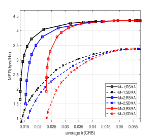
Figure 1: The trade-off performance under different
numbers of targets. $N_{t}=4$, $N_{r}=9$, $K=4$,
$N=1024$, $\mathrm{SNR}_{radar}=-20\ \mathrm{dBm}$.

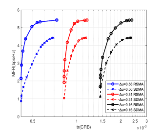
Figure 2: The trade-off performance under different
angle difference. $N_{t}=4$, $N_{r}=5$, $K=4$,
$M=2$, $N=256$, $\mathrm{SNR}_{radar}=10\ \mathrm{dBm}$.

Figure 3: Capon estimation based on the RSMA
-assisted ISAC beamforming.

In this section, we demonstrate the performance of the proposed RSMA-assisted multi-user multi-target ISAC model. The respective performance metrics for communication and sensing are the MMF rate and the trace of the weighted CRB, which is expressed as $\mathrm{tr}(\mathbf{\Lambda}\mathbf{F}^{-1})$, where $\mathbf{\Lambda}=\mathrm{diag}([\lambda_{1},\dots,\lambda_{4M}]^{T})\in\mathbb{C}^{4M\times 4M}$ denotes the weights of different target parameters. Unless otherwise specified, the weights are set as $\left\{\lambda_{i}\right\}_{i=1}^{4M}=1$[8]. When varying numbers of targets are considered, for fairness of comparison, we consider the sensing performance metric as the average trace of CRB defined by $\mathrm{tr}(\mathbf{F}^{-1})/M$.

Unless otherwise specified, we consider the scenario where the BS is equipped with $N_{t}=4$ transmit antennas and $N_{r}=9$ receive antennas and it serves $K=4$ communication users. The total power budget at the BS is $P=20\ \mathrm{dBm}$ and we assume $\sigma_{c}^{2}=0\ \mathrm{dBm}$ without loss of generality. The SNR of radar is calculated by $\mathrm{SNR}_{radar}=|\alpha|P/\sigma_{s}^{2}=-20\ \mathrm{dBm}$, where $|\alpha|=|\{\alpha_{m}\}_{m=1}^{M}|=1,\forall m\in\mathcal{M}$. Consider $N=1024$ radar pulse blocks in one CPI. The channels between the BS and the communication users are assumed to be Rayleigh fading with each entry following the complex Gaussian distribution as $\mathcal{CN}(0,1)$. We consider 7 different targets, among which target 1-3 are located at 45^∘, 30^∘, 15^∘ with velocities of 10 $\mathrm{m/s}$, 14 $\mathrm{m/s}$, 18 $\mathrm{m/s}$, respectively. Target 4-7 are at 0^∘, 34^∘, 18^∘, 9^∘ with the same velocity of 10 $\mathrm{m/s}$. We use linearly precoded SDMA as a baseline, which is achieved through disabling the common stream of RSMA. The results are averaged over 100 channel realizations.

Fig. 3 illustrates the trade-off performance between communication and sensing when $M=1$ (target 1), $M=2$ (target 1-2) and $M=3$ (target 1-3). We observe that RSMA exhibits an explicit trade-off region gain over SDMA. Attributing to the additional degree-of-freedom (DoF) introduced by the common stream, RSMA achieves a superior MMF rate than SDMA at the rightmost corner point. As the number of targets increases, the trade-off regions of both RSMA and SDMA become worse since the loss of the beamforming power at each single target. Surprisingly, we observe that RSMA is capable of detecting more targets than SDMA while maintaining the QoS of the communication users, thus showing the great potential of RSMA to enhance the sensing functionality.

Fig. 3 shows the trade-off comparison between RSMA and SDMA when the angle difference between $M=2$ targets defined by $\Delta u=\sin(\theta_{1})-\sin(\theta_{2})$ varies. To explicitly investigate the influence of the angle difference between the target, $\Delta f=\mathcal{F}_{D_{1}}-\mathcal{F}_{D_{2}}=0$ is considered. There are $N_{t}=4$ transmit antennas and $N_{r}=5$ receive antennas at the BS. We set $\mathrm{SNR}_{radar}=10\ \mathrm{dBm}$, $N=256$ and generate $K=4$ communication user channels randomly by following the complex Gaussian distribution[2]. As the angle difference grows from $\Delta u=0.16$ (target 7, 4), $\Delta u=0.31$ (target 6, 4) to $\Delta u=0.56$ (target 5, 4), the sensing metric $\mathrm{tr(CRB)}$ tends to become lower, owing to the decrease of the interference between the radar echo signals at the receiver. We observe that under various angle differences, the proposed RSMA consistently outperforms SDMA.

To further evaluate the sensing capability of the proposed ISAC system, we employ the Capon beamformer to estimate the angles and velocities of the targets, which maximizes SINR and reduces noise and interference while ensuring that the desired signal is not distorted. The Capon beamformer $\mathbf{w}_{p}\in\mathbb{C}^{N_{r}\times 1}$ is expressed as

$$\mathbf{w}_{p}(\theta)=\frac{\mathbf{R}_{y}^{-1}\mathbf{b}(\theta)}{\mathbf{b}^{H}(\theta)\mathbf{R}_{y}^{-1}\mathbf{b}(\theta)},$$ (18)

where $\mathbf{R}_{y}=\frac{1}{N}\sum_{n\in\mathcal{N}}\mathbf{y}_{s}[n]\mathbf{y}_{s}[n]^{H}$ is the covariance of the received signal. The Capon estimation of the complex reflection coefficient is defined as the minimizer of the following cost-function

$${\hat{\alpha}}(\theta,v) =\mathop{\mathrm{argmin}}_{\alpha}E\big{\{}|\mathbf{w}_{p}^{H}(\theta)\mathbf{y}_{s}[n]$$ (19)

$$-\mathbf{w}_{p}^{H}(\theta)\alpha e^{j2\pi\mathcal{F}_{D}nT}\mathbf{b}(\theta)\mathbf{a}^{T}(\theta)\mathbf{x}[n]|^{2}\big{\}}$$

$$=E\left\{\frac{\mathbf{w}_{p}^{H}(\theta)\mathbf{y}_{s}[n]\mathbf{x}^{H}[n]\mathbf{a}^{\ast}(\theta)e^{-j2\pi\mathcal{F}_{D}nT}}{\mathbf{a}^{T}(\theta)\mathbf{x}[n]\mathbf{x}^{H}[n]\mathbf{a}^{\ast}(\theta)}\right\}.$$

Substituting (18) into (19), we have

$$\hat{\alpha}(\theta,v) =\frac{\mathbf{b}^{H}(\theta)\mathbf{R}_{y}^{-1}\mathbf{Y}_{s}\mathbf{D}\mathbf{X}^{H}\mathbf{a}^{\ast}(\theta)}{\mathbf{b}^{H}(\theta)\mathbf{R}_{y}^{-1}\mathbf{b}(\theta)p(\theta)N},$$ (20)

where $p(\theta)=\mathbf{a}^{T}(\theta)\mathbf{R}_{x}\mathbf{a}^{\ast}(\theta)$ is the transmit beam pattern, $\mathbf{Y}_{s}=[\mathbf{y}_{s}[1],\dots,\mathbf{y}_{s}[N]]$, $\mathbf{X}=[\mathbf{x}[1],\dots,\mathbf{x}[N]]$, $\mathbf{D}=\mathrm{diag}([e^{-j2\pi\mathcal{F}_{D}T},\dots,e^{-j2\pi\mathcal{F}_{D}NT}]^{T})$. Obtaining $\hat{\alpha}$ at each grid point of $(\theta,v)$ requires two dimension calculation as [9]

$$\{\theta_{m},v_{m}\}_{m=1}^{M}=\mathop{\mathrm{argmax}}_{\theta,v}|\hat{\alpha}(\theta,v)|^{2}.$$ (21)

Therefore, we obtain $M$ peak points corresponding to the $M$ targets. Fig. 3 shows two peak points, which correspond to the targets 4-5. The precoding matrix used here is the optimized solution of (17) when $N_{t}=4$, $N_{r}=5$, $\mathrm{SNR}_{radar}=10\ \mathrm{dBm}$, $N=256$, and $\mu=10^{-3}$. The parameters of the two moving targets are correctly estimated, implying the high detection accuracy of RSMA.

VI Conclusion

This work initiates the study of RSMA in a mono-static ISAC system with multiple communication users and multiple sensing targets. We derive a general CRB sensing metric which embraces the estimation of angular direction, complex reflection coefficient, and Doppler frequency for multiple targets. By designing the transmit waveform to maximize the MMF rate of multiple users and minimize the largest eigenvalue of CRB of multiple moving targets, we show that RSMA achieves a better communication and sensing trade-off than conventional linearly precoded SDMA in multi-user multi-target ISAC. Additionally, the trade-off gain of RSMA grows with increasing angle difference between targets. Therefore, we conclude that RSMA offers a highly effective interference management solution. It has great potential for synergizing with ISAC in future wireless networks.

Appendix

derivation of the FIM in (8)

CRB is the lower bound on the variance of unbiased estimators and is given by $\mathbf{CRB}=\mathbf{F}^{-1}$. The matrix $\mathbf{F}$ is related to four target parameters $\mathbf{\xi}_{m}=\left\{\theta_{m},\alpha_{\Re_{m}},\alpha_{\Im_{m}},\mathcal{F}_{D_{m}}\right\}^{T}$, $\forall m\in\mathcal{M}$. With definition of $\mathbf{v}[n]=\mathbf{y}_{s}[n]-\mathbf{z}_{s}[n]=\mathbf{B}\mathbf{U}\mathbf{E}[n]\mathbf{A}^{T}\mathbf{x}[n]$, we note that

$$\mathbf{F}_{\mathcal{F}_{D_{i}}\mathcal{F}_{D_{j}}}=2\mathrm{Re}\Big{[}\mathrm{tr}\Big{\{}\sum_{n\in\mathcal{N}}\frac{\partial\mathbf{v}[n]^{H}}{\partial\mathcal{F}_{D_{i}}}\mathbf{Q}^{-1}\frac{\partial\mathbf{v}[n]}{\partial\mathcal{F}_{D_{j}}}\Big{\}}\Big{]},\forall i,j\in\mathcal{M},$$ (22)

the partial derivative can be calculated as

$$\frac{\mathbf{v}[n]}{\partial\mathcal{F}_{D_{i}}}=\mathbf{B}\mathbf{U}\left(j2\pi nT\right)\mathbf{E}[n]\mathbf{e}_{i}\mathbf{e}_{i}^{T}\mathbf{A}^{T}\mathbf{x}[n],\forall i\in\mathcal{M},$$ (23)

where $\mathbf{e}_{i}$ is the $i$th column of $\mathbf{I}_{K}$. Since $\mathrm{tr}(\mathbf{A}\mathbf{B})=\mathrm{tr}(\mathbf{B}\mathbf{A})$ and $\mathbf{U}$, $\mathbf{E}[n]$ are diagonal matrices, (22) can be rewritten as

$$\mathbf{F}_{\mathcal{F}_{D_{i}}\mathcal{F}_{D_{j}}} =2\mathrm{Re}\Big{[}\mathrm{tr}\Big{\{}\sum_{n\in\mathcal{N}}\big{(}\mathbf{B}\mathbf{U}\left(j2\pi nT\right)\mathbf{E}[n]\mathbf{e}_{i}\mathbf{e}_{i}^{T}\mathbf{A}^{T}\times$$

$$\mathbf{x}[n]\big{)}^{H}\mathbf{Q}^{-1}\left(\mathbf{B}\mathbf{U}\left(j2\pi nT\right)\mathbf{E}[n]\mathbf{e}_{j}\mathbf{e}_{j}^{T}\mathbf{A}^{T}\mathbf{x}[n]\right)\Big{\}}\Big{]}$$

$$=2\mathrm{Re}\Big{[}\mathrm{tr}\Big{\{}\sum_{n\in\mathcal{N}}\mathbf{e}_{i}^{T}\mathbf{B}^{H}\mathbf{Q}^{-1}\mathbf{B}\mathbf{e}_{j}\mathbf{e}_{j}^{T}\mathbf{U}\mathbf{E}[n]j2\pi nT$$

$$\times\mathbf{A}^{T}\mathbf{x}[n]\mathbf{x}[n]^{H}\mathbf{A}^{\ast}\mathbf{E}^{H}[n]\left(-j2\pi nT\right)\mathbf{U}^{H}\mathbf{e}_{i}\Big{\}}\Big{]}$$

$$=2\mathrm{Re}\Big{\{}(\mathbf{B}^{H}\mathbf{Q}^{-1}\mathbf{B})_{ij}(\mathbf{U}^{\ast}\mathbf{A}^{H}\mathbf{R}_{x}^{\ast}\mathbf{A}\mathbf{U})_{ij}$$

$$\times(\mathbf{\Sigma}_{3})_{ij}\Big{\}},\forall i,j\in\mathcal{M},$$ (24)

where $(\cdot)_{ij}$ refers to the $i$th row and $j$th column element of the matrix. Thus we obtain $\mathbf{F}_{\mathcal{F}_{D}\mathcal{F}_{D}}=2\mathrm{Re}(\mathbf{F}_{44})$, with $\mathbf{F}_{44}$ specified in (9). Other terms of FIM can be calculated in the same way with the corresponding partial derivative. Hence, we obtain the FIM in (8).

References

• [1] F. Liu et al., “Cramér-rao bound optimization for joint radar-communication beamforming,” IEEE Trans. Signal Process., vol. 70, pp. 240–253, 2022.
• [2] C. Xu et al., “Rate-splitting multiple access for multi-antenna joint radar and communications,” IEEE J. Sel. Top. Signal Process., vol. 15, no. 6, pp. 1332–1347, 2021.
• [3] R. Cerna-Loli et al., “A rate-splitting strategy to enable joint radar sensing and communication with partial CSIT,” in Proc. IEEE Int. Workshop Signal Process. Adv. Wireless Commun. (SPAWC), Sep. 2021, pp. 491–495.
• [4] L. Yin et al., “Rate-splitting multiple access for dual-functional radar-communication satellite systems,” in Proc. IEEE Wireless Commun. Netw. Conf. (WCNC), Apr. 2022, pp. 1–6.
• [5] ——, “Rate-splitting multiple access for 6G–part II: Interplay with integrated sensing and communications,” IEEE Commun. Lett., vol. 26, no. 10, pp. 2237–2241, 2022.
• [6] Y. Mao et al., “Rate-splitting multiple access: Fundamentals, survey, and future research trends,” IEEE Commun. Surv. Tutorials, vol. 24, no. 4, pp. 2073–2126, 2022.
• [7] J. Li et al., “Range compression and waveform optimization for MIMO radar: A Cramér-rao bound based study,” IEEE Trans. Signal Process., vol. 56, no. 1, pp. 218–232, 2008.
• [8] M. Zhu et al., “Information and sensing beamforming optimization for multi-user multi-target MIMO ISAC systems,” EURASIP J. Adv. Signal Process., vol. 2023, 2023.
• [9] S. Jardak et al., “Low complexity moving target parameter estimation for MIMO radar using 2D-FFT,” IEEE Trans. Signal Process., vol. 65, no. 18, pp. 4745–4755, 2017.