How movement bias to attractive regions determines population spread and critical habitat size

Abstract

Ecologists have long investigated how the demographic and movement parameters of a population determine its spatial spread and the critical habitat size that can sustain it. Yet, most existing models make oversimplifying assumptions about individual movement behavior, neglecting how landscape heterogeneity influences dispersal. We relax this assumption and introduce a reaction-advection-diffusion model that describes the spatial density distribution of a population with space-dependent movement bias toward preferred regions, including avoidance of degraded habitats. In this scenario, the critical habitat size depends on the spatial location of the habitat edges with respect to the preferred regions and on the intensity of the movement bias components. In particular, we identify parameter regions where the critical habitat size decreases when diffusion increases, a phenomenon known as the “drift paradox”. We also find that biased movement toward low-quality or highly populated regions can reduce the population size, therefore creating ecological traps. Our results emphasize the importance of species-specific movement behavior and habitat selection as drivers of population dynamics in fragmented landscapes and, therefore, the need to account for them in the design of protected areas.

1 Introduction

Habitat destruction and fragmentation result in smaller and more isolated suitable habitat patches where extinctions are more likely to occur (Lord and Norton,, 1990; Franklin et al.,, 2002; Nauta et al.,, 2022). The viability of a population in each of these patches depends on the balance between growth inside the patch and population losses, mainly stemming from dispersal through habitat edges. The interplay between these two processes sets the minimum area required to sustain the population and defines a patch-size threshold (Kierstead and Slobodkin,, 1953). Thus, understanding the interaction between demographic and dispersal processes is key to determining critical patch sizes across species, which has important implications for conservation, such as in the design of protected areas or ecological corridors (Cantrell and Cosner,, 1999; Ibagon et al.,, 2022). Additionally, determining the expected spatial pattern of population density in patches larger than the critical size can improve understanding of population responses to further habitat destruction.

The importance of critical patch sizes and population spread in finite habitat patches has led researchers to test model predictions in microcosm experiments using microbial populations (Lin et al.,, 2004; Perry,, 2005) as well as in large-scale experiments and observations (Turner,, 1996; Ferraz et al.,, 2003; Pereira and Daily,, 2006). Despite the biological understanding gained from these and other empirical studies, key aspects of complexity remain absent from theoretical modeling of critical patch size phenomena. The most common models to determine critical habitat sizes consist of a reaction-diffusion equation describing the spatio-temporal dynamics of a population density in a bounded region. Within this family of models, the simplest ones assume purely diffusive dispersal coupled with exponential growth and are commonly called KISS models (Skellam,, 1951; Kierstead and Slobodkin,, 1953). Due to these highly simplified assumptions, KISS models lead to analytical expressions for the critical patch size.

More recently, researchers have refined movement descriptions by including space-dependent diffusion within the patch (Dos Santos et al.,, 2020; Colombo and Anteneodo,, 2018), responses to habitat edges (Fagan et al.,, 1999; Maciel and Lutscher,, 2013; Cronin et al.,, 2019), and various sources of non-random movement, such as a constant external flow (Pachepsky et al.,, 2005; Ryabov and Blasius,, 2008; Vergni et al.,, 2012; Speirs and Gurney,, 2001) or a chemoattractant secreted by the population (Kenkre and Kumar,, 2008). Other studies have explored more complex growth dynamics, such as Allee effects (Alharbi and Petrovskii,, 2016; Cronin et al.,, 2020), time-varying environments (Zhou and Fagan,, 2017), or heterogeneity in population growth, either through time-dependent demographic rates (Ballard et al.,, 2004; Colombo and Anteneodo,, 2016) or by introducing a finer spatial structure of habitat quality within the patch (Cantrell and Cosner,, 2001; Maciel and Lutscher,, 2013; Fagan et al.,, 2009). Finally, a few studies have combined space-dependent demographic rates with migration toward higher quality regions within the patch, in the presence of an environmental gradient, to determine critical patch sizes (Cantrell and Cosner,, 1991, 2001; Cantrell et al.,, 2006) or population spatial distributions depending on the type of boundary conditions (Belgacem and Cosner,, 1995).

Despite this significant endeavor to refine classical KISS models, some movement features which are present in most species and which directly impact population spread remain underexplored. For example, individuals often show a tendency to move toward certain habitat regions where they concentrate, which makes population ranges smaller than the total amount of habitat available (Van Moorter et al.,, 2016; Kapfer et al.,, 2010). While a considerable effort has focused on understanding how and why individuals show these patterns of space use (Nathan et al.,, 2008; Jeltsch et al.,, 2013), their population-level consequences, especially in fragmented landscapes, have been less explored. Motivated by colonial central-place foragers such as ants, beavers, and colonial seabirds, one particular study obtained, numerically, the critical patch size when the home-range centers for all the individuals in the population are at the center of the habitat patch (Fagan et al.,, 2007). Overall, however, the lack of a more general theoretical framework limits the current understanding of how habitat selection within a fragmented landscape determines the spatial distribution and critical patch size for a given population.

Here we take a first step to fill this theoretical gap by extending classical KISS models to account for space-dependent deterministic movement. We study how this additional movement component influences population spread in a heterogeneous one-dimensional landscape and the critical habitat patch size that ensures population survival. We consider the simple one-dimensional scenario with a finite high-quality habitat patch embedded in a low-quality “matrix” with high mortality. Using both numerical and analytical methods, we measure critical patch size and spatial patterns of population density for different matrix mortality levels. We also vary the intensity of two deterministic space-dependent movement components relative to random dispersal: a bias to preferred landscape locations and avoidance of degraded habitats. We find that the total population lost due to habitat degradation and the critical patch size depend nonlinearly on the parameters that control the different movement components as well as on the spatial distribution of habitat relative to the landscape regions where individuals move more slowly. Overall, our results emphasize the importance of incorporating covariates between movement behavior and landscape features when investigating population dynamics in heterogeneous landscapes.

2 Material and Methods

2.1 Model formulation

We consider a one-dimensional heterogeneous landscape with a habitat patch embedded in an infinite matrix (see Fig. 1a). The left and right habitat patch edges are located at $x=x_{\mbox{\tiny{L}}}$ and $x=x_{\mbox{\tiny{R}}}$, respectively, and the habitat patch size is $L=|x_{\mbox{\tiny{R}}}-x_{\mbox{\tiny{L}}}|$. The landscape is occupied by a single-species population, which we describe via a continuous density field $u(x,t)$. This population density changes in space and time due to demographic processes and dispersal. For the birth/death dynamics, we assume that the population follows logistic growth with net reproduction rate $r$ and intraspecific competition intensity $\gamma$. The net growth rate is constant within each type of region but different between regions: $r(x)=r_{\mbox{\tiny{H}}}>0$ inside the habitat patch (high-quality, low-mortality region) and $r(x)=r_{\mbox{\tiny{M}}}<0$ in the matrix (low-quality, high-mortality region). The matrix mortality rate $r_{\mbox{\tiny{M}}}$ defines the degree of habitat degradation, with the limit $r_{\mbox{\tiny{M}}}\rightarrow-\infty$ representing complete habitat destruction. For finite mortality rates, whether an individual dies in the matrix or not is determined by the mortality rate itself and the time the individual spends in the matrix. Therefore, when the matrix is not immediately lethal, the population density outside the habitat patch is not zero. For dispersal, we consider two different movement components: random dispersal with constant diffusion coefficient $D$, and a deterministic tendency of individuals to move toward attractive regions with space-dependent velocity $v(x)$, therefore accounting for the effect of landscape heterogeneity in movement behavior. Importantly, this attractive term in our model generates movement bias toward regions that are not necessarily of higher habitat quality. The actual velocity of an individual is thus equal to $v(x)$ plus a stochastic contribution that comes from diffusion. Combining these demographic and movement processes, the dynamics of the population density is given by

$$\frac{\partial u(x,t)}{\partial t}=r(x)u(x,t)-\gamma u(x,t)^{2}+D\frac{\partial^{2}u(x,t)}{\partial x^{2}}-\frac{\partial}{\partial x}\bigg{(}v(x)u(x,t)\bigg{)}.$$ (1)

The functional form of the advection velocity $v(x)$ depends on landscape features, with attractive locations corresponding to $x$ coordinates with slower velocity. We consider two different types of attractive regions.

First, we incorporate a tendency to move toward an attractive location with velocity $v_{\mbox{\tiny{P}}}(x)$. This term could represent, for example, attraction toward a chemoattractant source or toward a special resource, such as a watering hole. We choose

$$v_{\mbox{\tiny{P}}}(x)=-\tau_{\mbox{\tiny{P}}}^{-1}(x-x_{\mbox{\tiny{P}}}),$$ (2)

where we assumed that the velocity at which individuals tend to move toward attractive landscape regions increases linearly with the distance to the focus of attraction. This is similar to how simple data-driven models for range-resident movement implement attraction to home-range center at the individual level (Dunn and Gipson,, 1977; Noonan et al.,, 2019). The prefactor $\tau_{\mbox{\tiny{P}}}^{-1}$ is the attraction rate toward the attractive location and defines the typical time that individuals take to re-visit $x_{\mbox{\tiny{P}}}$. In the following, we use $x_{\mbox{\tiny{P}}}=0$ in all our calculations, such that the locations of the habitat edges are measured relative to the focus of attraction.

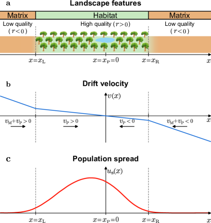
Figure 1: Model schematics. (a) Landscape features, showing a high-quality habitat ($r>0$) and an attractive location (represented as a watering hole at position $x=x_{\mbox{\tiny{P}}}=0$) surrounded by low-quality matrix regions ($r<0$). Habitat edges are located at $x=x_{\mbox{\tiny{L}}}$ and $x=x_{\mbox{\tiny{R}}}$. In this example, $x_{\mbox{\tiny{R}}}$ is positive. The total habitat size is $L=|x_{\mbox{\tiny{R}}}-x_{\mbox{\tiny{L}}}|$. (b) Spatial dependence of the drift velocity (deterministic movement component). Velocity $v_{\mbox{\tiny{P}}}$ points to the attractive location [Eq. 2]. For individuals in the matrix, an additional term ($v_{\mbox{\tiny{M}}}$) points to the edges [Eq. 3]. (c) Emerging stationary population density distribution $u_{\mbox{\tiny{s}}}(x)$, peaking to the left of $x=0$.

Second, we consider that individuals in the matrix tend to return to the habitat patch with velocity $v_{\mbox{\tiny{M}}}(x)$, and therefore, we incorporate an additional attraction term biasing movement from the matrix toward its closest habitat edge. Again, we consider a linear spatial dependence, but now only for individuals in the matrix:

$$v_{\mbox{\tiny{M}}}(x)=\begin{cases}-\tau^{-1}_{\mbox{\tiny{M}}}(x-x_{\mbox{\tiny{L}}}),&x<x_{\mbox{\tiny{L}}}\\ 0,&x_{\mbox{\tiny{L}}}\leq x\leq x_{\mbox{\tiny{R}}}\,.\\ -\tau^{-1}_{\mbox{\tiny{M}}}(x-x_{\mbox{\tiny{R}}}),&x>x_{\mbox{\tiny{R}}}\end{cases}$$ (3)

The prefactor $\tau^{-1}_{\mbox{\tiny{M}}}$ is the edge attraction rate that modulates the strength of the matrix-to-habitat attraction $v_{\mbox{\tiny{M}}}(x)$. In the habitat, $v_{\mbox{\tiny{M}}}(x)=0$, whereas in the matrix, it is equal to $\tau_{\mbox{\tiny{M}}}^{-1}$ multiplied by the distance to the closest edge. Moreover, the velocity $v_{\mbox{\tiny{M}}}(x)$ always points toward the habitat patch, therefore biasing the movement of the individuals in the matrix toward the habitat-matrix edges. This matrix avoidance drift assumes that individuals remain aware of the direction in which the favorable habitat is located, which extends previous models for movement response to habitat edges that act only at the habitat-matrix boundary (Fagan et al.,, 1999; Maciel and Lutscher,, 2013; Cronin et al.,, 2019).

Putting together the movement toward the attractive location and the matrix avoidance bias, we obtain a velocity of the form $v(x)=v_{\mbox{\tiny{P}}}(x)+v_{\mbox{\tiny{M}}}(x)$ (see Fig. 1b for $v(x)$ and Fig. 1c for the population spread emerging from it). We provide a summary of the model parameters in Table 1.

Sym.	Parameter	Dimensions
$r_{\mbox{\tiny{H}}}$	Habitat net growth rate	time-1
$r_{\mbox{\tiny{M}}}$	Matrix net rate	time-1
$\gamma$	Intensity of intraspecific compet.	(time $\times$ density)-1
$D$	Diffusion coefficient	space2/time
$x_{\mbox{\tiny{P}}}$	Center attractive location	space
$x_{\mbox{\tiny{L}}}$	Position of left habitat edge	space
$x_{\mbox{\tiny{R}}}$	Position of right habitat edge	space
$\tau_{\mbox{\tiny{P}}}^{-1}$	Attraction rate to attractive location	time-1
$\tau_{\mbox{\tiny{M}}}^{-1}$	Matrix-to-habitat attraction rate	time-1

Table 1: Summary of model parameters with symbols and dimensions. Units are arbitrary. Specific values are provided in figure captions.

2.2 Model analysis

We analyze the stationary solutions of Eq. (1) using a combination of semi-analytical linear stability analysis and numerical simulations of the full nonlinear equation. We use both approaches in the $r_{\mbox{\tiny{M}}}\rightarrow-\infty$ limit and perform only numerical simulations in the more general case with finite $r_{\mbox{\tiny{M}}}$.

2.2.1 Linear stability analysis of the extinction state when $r_{\mbox{\tiny{M}}}\rightarrow-\infty$

In the $r_{\mbox{\tiny{M}}}$$\rightarrow$$-\infty$ limit, individuals die instantaneously upon reaching the matrix, and we can replace the dynamics of the population density in the matrix by absorbing boundary conditions at the habitat edges, $u(x_{\mbox{\tiny{L}}},t)=u(x_{\mbox{\tiny{R}}},t)=0$. In this regime, the movement component that attracts individuals to the habitat edge, $v_{\mbox{\tiny{M}}}$, has no effect on the dynamics, and we can perform a linear stability analysis of the extinction solution $u(x,t\rightarrow\infty)\equiv u_{s}(x)=0$ to determine the habitat configurations $(x_{\mbox{\tiny{L}}},x_{\mbox{\tiny{R}}})$ that lead to population extinction for a given set of movement parameters. To perform this linear stability analysis, we neglect the quadratic term in the logistic growth and take the limit $t\rightarrow\infty$ in Eq. 1, which is equivalent to setting $\partial_{t}u(x,t)=0$. In this limit, Eq. 1 becomes an ordinary differential equation with solution

$$u_{\mbox{\tiny{s}}}(x)=\exp\left(-\frac{x^{2}}{2\tau_{\mbox{\tiny{P}}}D}\right)\left[aH_{r\tau_{\mbox{\tiny{P}}}}\left(\frac{x}{\sqrt{2D\tau_{\mbox{\tiny{P}}}}}\right)+\,b\,\,_{1}F_{1}\left(-\frac{r\tau_{\mbox{\tiny{P}}}}{2};\frac{1}{2};\frac{x^{2}}{2D\tau_{\mbox{\tiny{P}}}}\right)\right],$$ (4)

where $a$ and $b$ are constants that we can obtain from the boundary conditions. ${}_{1}F_{1}$ is the confluent hypergeometric function of the first kind, and $H_{n}(x)$ is the Hermite polynomial, with $n$ being a real, not necessarily integer, number (Arfken and Weber,, 1999). Imposing absorbing boundary conditions at the habitat edges on Eq. 4, we obtain a system of two equations for $a$ and $b$ that we can use to determine the stability of the solution $u_{s}(x)=0$. For this system of equations to have non-trivial solutions (that is, different from $a=b=0$), its determinant has to be zero. With this condition for the determinant and assuming that $x_{\mbox{\tiny{L}}}$ is fixed, we obtain a transcendental equation in $x_{\mbox{\tiny{R}}}$ that we can solve numerically to obtain the critical location of the right habitat edge, $x_{\mbox{\tiny{R,C}}}$.

2.2.2 Numerical solution of the nonlinear model equation

We perform all numerical simulations using a central Euler method starting from a random positive initial condition for $u$. In the $r_{\mbox{\tiny{M}}}\rightarrow-\infty$ limit, we further ensure that the initial condition obeys the absorbing boundary conditions at the habitat edges. We integrate Eq. 1 for a variety of habitat patch sizes keeping $x_{\mbox{\tiny{L}}}$ constant and decreasing $x_{\mbox{\tiny{R}}}$ systematically until the population reaches a stationary extinction state. Using this procedure, we can calculate $x_{\mbox{\tiny{R,C}}}$ and hence the critical patch size defined as the habitat patch size at which the steady-state total population transitions from non-zero to zero (see Fig. 2 for spatial patterns of population density as $x_{\mbox{\tiny{R}}}$ decreases, with $x_{\mbox{\tiny{R}}}>x_{\mbox{\tiny{R,C}}}$).

Finally, we also use these numerical solutions of Eq. 1 to measure population loss due to habitat degradation. For this purpose, we introduce a dimensionless quantity, $\eta$, defined as the total population size sustained by a finite habitat patch of size $L$ divided by the total population size sustained by an infinite habitat patch. Such remaining population fraction is thus

$$\eta\equiv\frac{N_{\mbox{\tiny{T}}}}{N_{\mbox{\tiny{T}}}^{\infty}},$$ (5)

where $N_{\mbox{\tiny{T}}}$ and $N_{\mbox{\tiny{T}}}^{\infty}$ are the total population sizes for finite and infinite habitat patches, respectively. We obtain these population sizes by integrating the population density over the entire landscape, including the matrix.

3 Results

3.1 Perfectly absorbing matrix: the $r_{\mbox{\tiny{M}}}\rightarrow-\infty$ limit

We first consider the simplest scenario in which individuals die instantaneously after they reach the habitat edges. In this limit, the population density is always zero in the matrix and, therefore, the movement component that biases individuals in the matrix toward the habitat edges is irrelevant. Movement is thus solely driven by random diffusion and the bias toward the attractive location $x=x_{\mbox{\tiny{P}}}=0$. In large habitat patches, space-dependent movement leads to the accumulation of population density very close to regions with slower movement. However, as the habitat patch decreases in size and regions with slower movement get closer to one of the habitat edges, the spatial pattern of population density changes due to mortality at the habitat edge and the maximum of population density shifts further away from the attractive location and towards the patch center (Fig. 2). This asymmetric pattern of space occupation due to space-dependent movement contrasts with well-known results for purely diffusive movement, for which population density reaches its maximum in the center of the habitat patch (Holmes et al.,, 1994), and significantly alters population loss owing to habitat degradation and the critical patch size.

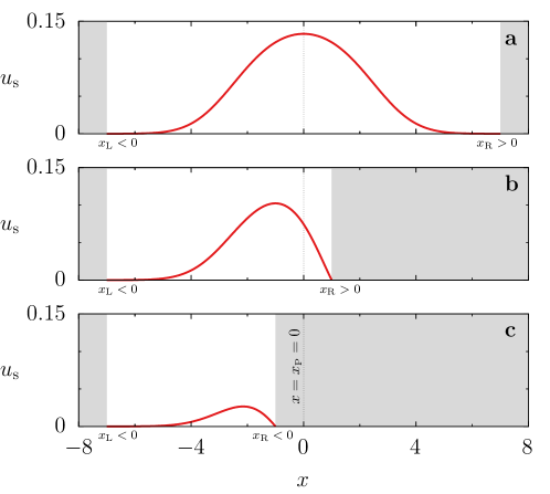
Figure 2: Stationary population density distribution $u_{\mbox{\tiny{s}}}(x)$ obtained from a numerical integration of Eq. 1. Space-dependence movement bias $v_{\mbox{\tiny{P}}}(x)$ is active and draws the population toward the attractive location $x=x_{\mbox{\tiny{P}}}=0$. (a) $x_{\mbox{\tiny{R}}}=7$ and $x_{\mbox{\tiny{L}}}=-7$, (b) $x_{\mbox{\tiny{R}}}=1$ and $x_{\mbox{\tiny{L}}}=-7$, and (c) $x_{\mbox{\tiny{R}}}=-1$ and $x_{\mbox{\tiny{L}}}=-7$. Other parameters: $r_{\mbox{\tiny{H}}}=0.1$, $\gamma=1$, $D=0.1$, $x_{\mbox{\tiny{P}}}=0$, and $\tau_{\mbox{\tiny{P}}}^{-1}=0.05$. Also, $r_{\mbox{\tiny{M}}}\rightarrow-\infty$. Gray regions represent the matrix.

First, to understand population loss due to habitat degradation, we use the remaining population fraction, $\eta$, defined in Eq. (5). This remaining population fraction is maximal when the attractive location is at the same distance from the two habitat edges, and it decays symmetrically about the line $x_{\mbox{\tiny{R}}}=-x_{\mbox{\tiny{L}}}$. Moreover, this decay is sharper for stronger bias toward the attractive location (Fig. 3 and  S1). Finally, when the distance between the attractive location and one of the habitat edges is sufficiently large, further increasing the habitat size does not change the remaining population fraction because population loss through habitat edges is negligible, except for $\tau_{\mbox{\tiny{P}}}^{-1}=0$.

Regarding the critical patch size, when the bias to the attractive location is strong, represented by higher values of $\tau_{\mbox{\tiny{P}}}^{-1}$, the population is localized around the attractive location $x_{\mbox{\tiny{P}}}=0$, and it goes extinct when the attractive location is within the habitat patch but close to one of its edges (Fig. 3a, b). When the bias to the attractive location decreases, however, the population can survive even if the attractive location is outside the habitat and the mortality in the matrix is infinite (Fig. 2c and 3c). This scenario would correspond to a situation where habitat destruction places the attractive location outside the habitat and individuals have not adapted their movement behavior to this landscape modification. As a result, individuals preferentially move toward regions with low habitat quality, which can be understood as an example of an ecological trap (Robertson and Hutto, 2006a, ; Weldon and Haddad,, 2005; Lamb et al.,, 2017).

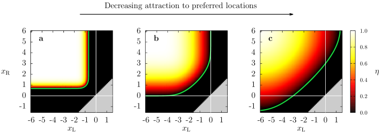
Figure 3: Remaining population fraction, $\eta$, for different habitat configurations $(x_{\mbox{\tiny{L}}},x_{\mbox{\tiny{R}}})$. (a) $\tau_{\mbox{\tiny{P}}}^{-1}=0.05$, (b) $\tau_{\mbox{\tiny{P}}}^{-1}=0.1$, and (c) $\tau_{\mbox{\tiny{P}}}^{-1}=0.5$. Other parameters: $r_{\mbox{\tiny{H}}}=0.1$, $D=0.1$, and $\gamma=1$. Also, $r_{\mbox{\tiny{M}}}\rightarrow-\infty$. The solid green line shows the critical patch size obtained with the linear stability analysis of the model equation.

To further investigate how the distance between the attractive location and the habitat edges determines the critical patch size for different movement parameters, we calculate the critical location of the right habitat edge $x_{\mbox{\tiny{R,C}}}$ assuming that the left habitat edge is fixed and far from the attractive location. In these conditions, if $x_{\mbox{\tiny{R}}}$ is also large, mortality through the left edge is negligible, but it becomes significant for smaller habitat patches. This setup mimics a situation where an initially large patch shrinks due to continued habitat destruction, slowly enough that the population distribution is at equilibrium for each particular habitat configuration, until it reaches a critical size and the population collapses. We find that the critical patch size is a nontrivial function of the intensity of the movement bias toward the attractive location and the distance between habitat edges and the attractive location. When $\tau_{\mbox{\tiny{P}}}^{-1}=0.1$, $x_{\mbox{\tiny{R,C}}}=0$ regardless of the value of $D$.

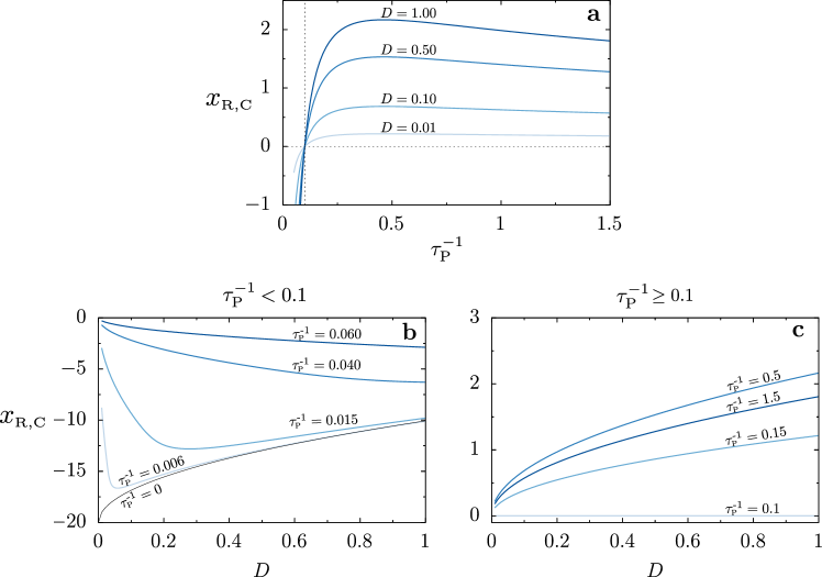
Figure S2: Critical location of the right habitat edge $x_{\mbox{\tiny{R,C}}}$ (a) as a function of $\tau_{\mbox{\tiny{P}}}^{-1}$, and as a function of $D$ for (b) $\tau_{\mbox{\tiny{P}}}^{-1}<0.1$ and (c) $\tau_{\mbox{\tiny{P}}}^{-1}>0.1$. Other parameters: $r_{\mbox{\tiny{H}}}=0.1$, $\gamma=1$, $r_{\mbox{\tiny{M}}}\rightarrow-\infty$, and $x_{\mbox{\tiny{L}}}=-20$.

For $\tau_{\mbox{\tiny{P}}}^{-1}>0.1$, movement bias is so strong that the attractive location must be within the habitat patch to avoid individuals entering the matrix and dying at a rate that cannot be outbalanced by population growth within the habitat (red region in Fig. 4 and Fig. S2). Moreover, due to strong bias toward the attractive location, the population is concentrated around that location. Increasing the diffusion coefficient $D$ makes $x_{\mbox{\tiny{R,C}}}$ increase because the population spreads out, and individuals become more likely to reach the matrix and die. Increasing $\tau_{\mbox{\tiny{P}}}^{-1}$ from $\tau_{\mbox{\tiny{P}}}^{-1}=0.1$ for a fixed diffusion coefficient $D$, we find a non-monotonic relationship between $x_{\mbox{\tiny{R,C}}}$ and $\tau_{\mbox{\tiny{P}}}^{-1}$. First, the critical patch size increases with $\tau_{\mbox{\tiny{P}}}^{-1}$ because the population concentrates around the attractive location and are more likely to reach the matrix and die. For even higher attraction rate, the population concentrates very narrowly around the attractive location and individuals do not reach the habitat edge. As a result, the critical patch size decreases with $\tau_{\mbox{\tiny{P}}}^{-1}$.

For $\tau_{\mbox{\tiny{P}}}^{-1}<0.1$, $x_{\mbox{\tiny{R,C}}}$ is negative, which means that the population can persist even when the attractive location is in the matrix (blue region in Fig. 4). In this low-$\tau_{\mbox{\tiny{P}}}^{-1}$ regime, $x_{\mbox{\tiny{R,C}}}$ increases with $\tau_{\mbox{\tiny{P}}}^{-1}$ because less random movement increases the relative contribution of the movement bias to the population flux through the edge. Similarly, the critical patch size decreases with increasing $D$ for values of $\tau_{\mbox{\tiny{P}}}^{-1}$ not too far from $\tau_{\mbox{\tiny{P}}}^{-1}=0.1$. This negative correlation between critical patch size and diffusion appears because a more random movement reduces the tendency of individuals to cross the habitat edge (see Fig. S2b for curves of $x_{\mbox{\tiny{R,C}}}$ versus $D$ with fixed $\tau_{\mbox{\tiny{P}}}^{-1}$). This phenomenon, known as the "drift paradox," has been previously observed in organisms inhabiting streams, rivers, and estuaries where downstream drift is continuously present and extinction is inevitable in the absence of diffusion (Pachepsky et al.,, 2005; Speirs and Gurney,, 2001). However, as $D$ continues to increase and random diffusion dominates dispersal, the critical patch size increases due to population loss via diffusion through both habitat edges. Finally, for very low values of $\tau_{\mbox{\tiny{P}}}^{-1}$, diffusion controls the population flux through habitat edges and the behavior of the critical patch size converges to the theoretical prediction of the purely diffusive case, $L_{\mbox{\tiny{C}}}^{\mbox{\tiny{D}}}=\pi\sqrt{D/r_{\mbox{\tiny{H}}}}$ (Kierstead and Slobodkin,, 1953).

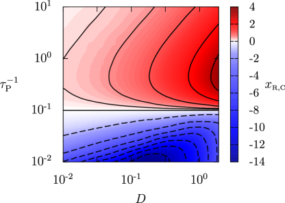
Figure 4: Critical location of the right habitat edge $x_{\mbox{\tiny{R,C}}}$ as a function of $\tau_{\mbox{\tiny{P}}}^{-1}$ and $D$. Parameter values: $r_{\mbox{\tiny{H}}}=0.1$, $\gamma=1$, $x_{\mbox{\tiny{L}}}=-20$, $r_{\mbox{\tiny{M}}}\rightarrow-\infty$.

3.2 Partially absorbing matrix and the effect of matrix-to-habitat bias

Considering finite $r_{\mbox{\tiny{M}}}$ allows us to investigate how changes in movement behavior, once individuals reach the matrix, can alter the spatial pattern of population density and the critical patch size. If individuals in the matrix do not tend to return to the habitat ($\tau^{-1}_{\mbox{\tiny{M}}}\approx 0$), the population density decays into the matrix exponentially, and the critical patch size increases with matrix mortality rate Fig. 5; Ludwig et al., 1979, Ryabov and Blasius, 2008.

For low values of $\tau^{-1}_{\mbox{\tiny{M}}}$, the tendency to return from the matrix to the habitat edges reduces how much the population penetrates the matrix and increases the population density inside the habitat, especially close to the edges (Fig. 5a). The spatial distribution of the population has a skewness that reaches its maximum when the attractive location is in the matrix (Fig. 5b). For large enough $\tau^{-1}_{\mbox{\tiny{M}}}$, the edges act as almost hard walls, and the term representing the tendency to return from the matrix to the nearest habitat edge behaves effectively as reflecting boundary conditions in Eq. (1). In this limit, the population survives for any habitat size (Maciel and Lutscher,, 2013).

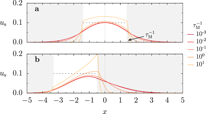
Figure 5: Stationary population density distribution $u_{\mbox{\tiny{s}}}(x)$ for the scenario with matrix-to-habitat attraction and attraction to the preferred location $x=x_{\mbox{\tiny{P}}}=0$. The parameters are $L=2.8$, which is smaller than the $L_{\mbox{\tiny{C}}}$ for $r_{\mbox{\tiny{M}}}\rightarrow-\infty$, $\tau_{\mbox{\tiny{P}}}^{-1}=0.05$, $r_{\mbox{\tiny{M}}}=-10^{-3}$, and $\tau^{-1}_{\mbox{\tiny{M}}}$ increasing for lighter colors, as indicated. (a) $x_{\mbox{\tiny{R}}}=-x_{\mbox{\tiny{L}}}=1.4$ and (b) $x_{\mbox{\tiny{R}}}=-0.5$ and $x_{\mbox{\tiny{L}}}=-3.3$. Other parameters as in Fig. 2. In both panels, the dashed line corresponds to $u_{\mbox{\tiny{s}}}=r/\gamma$, which is the density inside the habitat for $\tau^{-1}_{\mbox{\tiny{M}}}\rightarrow\infty$ and $\tau^{-1}_{\mbox{\tiny{P}}}=0$, in which case $u_{\mbox{\tiny{s}}}=0$ in the matrix.

The accumulation of individuals around habitat edges suggests a potential tradeoff between a decrease in mortality in the matrix due to the attraction to habitat edges and an increase in intraspecific competition due to higher population densities in the habitat. To investigate the impact of this tradeoff on population loss due to habitat degradation, we measure the fraction of the population that remains for a given patch size relative to the value for an infinite habitat patch, $\eta$. We perform this measurement for several values of the matrix mortality rate $r_{\mbox{\tiny{M}}}$ and the returning rate to habitat edges $\tau^{-1}_{\mbox{\tiny{M}}}$, which are the two main parameters controlling the accumulation of population density at habitat edges. We consider a scenario with the attractive location at the center of the habitat patch, which is the limit where we have a weaker accumulation of individuals at habitat edges and, therefore, the regime in which the tradeoff between matrix mortality and intraspecific competition around habitat edges has a weaker effect on population dynamics.

At high matrix mortality rates, the population does not survive ($\eta=0$), except for very high returning rates $\tau^{-1}_{\mbox{\tiny{M}}}$ (Fig. 6). When the matrix mortality rate decreases, $\eta$ increases and remains a monotonically increasing function of $\tau^{-1}_{\mbox{\tiny{M}}}$. For $r_{\mbox{\tiny{M}}}$ closer to zero, however, $\eta$ becomes a non-monotonic function of $\tau^{-1}_{\mbox{\tiny{M}}}$. For these values of the matrix mortality rate, increasing the returning rate to habitat edges is initially detrimental to the total population size because it leads to higher intraspecific competition at the habitat edges, which outweighs the decrease in mortality in the matrix. In other words, the density distribution does not penetrate the matrix as far (Fig. 5a) while, inside the habitat, competition does not allow for a large enough increase in population, and so the total population decreases. Consequently, the habitat edge itself behaves as an ecological trap in this regime, and our model recovers a behavior similar to previous observations for insects (Ries and Fagan,, 2003; Ries et al.,, 2004). Above a critical value of $\tau^{-1}_{\mbox{\tiny{M}}}$ at which $\eta$ is minimal, further increasing the returning rate to habitat edges becomes beneficial for population persistence because now very few individuals enter the matrix and reduced matrix mortality outweighs the increased intraspecific competition at habitat edges. For infinite return rate $\tau^{-1}_{\mbox{\tiny{M}}}$, all the curves for different values of the matrix mortality rate $r_{\mbox{\tiny{M}}}$ converge to the same value because individuals do not penetrate the matrix. For $\tau^{-1}_{\mbox{\tiny{M}}}\rightarrow\infty$ and $\tau^{-1}_{\mbox{\tiny{P}}}=0$, one has $u_{\mbox{\tiny{s}}}=r/\gamma$ inside the habitat and $u_{\mbox{\tiny{s}}}=0$ in the matrix (dashed line in Fig. 5). The existence of a non-monotonic dependence of population size on advection strength is reminiscent of a behavior reported in a different scenario for a model with advection towards a continuous environmental gradient (Belgacem and Cosner,, 1995).

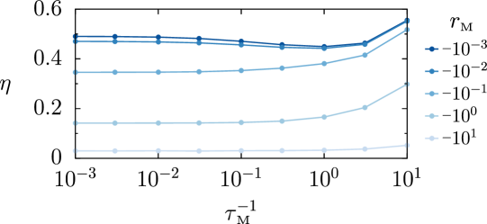
Figure 6: Ratio between the total population for $L$ and for $L\rightarrow\infty$, $\eta$, versus $\tau^{-1}_{\mbox{\tiny{M}}}$. $x_{\mbox{\tiny{R}}}=-x_{\mbox{\tiny{L}}}=1.4$ and values of $r_{\mbox{\tiny{M}}}$ as indicated, with lighter colors corresponding to larger absolute values of $r_{\mbox{\tiny{M}}}$. Other parameters as in Fig. 5.

4 Discussion

We studied the spatial dynamics of a population in a finite habitat surrounded by an infinite matrix, considering different ratios between matrix mortality and habitat reproduction rates. We additionally incorporated space-dependent deterministic movement through an advection term that attracts individuals toward specific landscape locations, including habitat edges. This advection term can create spatial distributions of population density that are asymmetric with respect to the center of the patch, especially when the patch size is small and attractive regions lie near habitat edges. This result could explain why, in certain species, populations tend to accumulate in the periphery of the species historical range following geographical range contraction (Channell and Lomolino, 2000b, ; Channell and Lomolino, 2000a, ). Moreover, our results show that both the habitat carrying capacity and critical size depend nonlinearly, sometimes non-monotonically, on movement and demographic parameters and the location of the habitat edges relative to regions of slower movement. Recent work has also found nonlinear and non-monotonic relationships between movement and landscape parameters underlying the stability of prey-predator systems in fragmented landscapes (Dannemann et al.,, 2018; Nauta et al.,, 2022). These findings emphasize the importance of untangling the various contributions determining individual movement, including environmental covariates, when designing conservation strategies such as refuges in fragmented landscapes or marine protected areas (Gerber et al.,, 2003; Gaston et al.,, 2002).

Specifically, for very low yet non-zero bias intensities, we find a range of values for the diffusion coefficient for which the critical habitat size decreases with increasing diffusion. This counterintuitive phenomenon is known as the “drift paradox” (Pachepsky et al.,, 2005). On the opposite limit, if movement bias toward the attractive location is very strong, the population becomes ultra-localized and its survival depends on whether the attractive site is in the habitat patch or the matrix; if it is in the patch, the population will persist, but if it is in the matrix, the population will go extinct. In between these two limits, for weak bias toward the attractive location, further increasing bias intensity increases the critical habitat size when the attractive site is inside the habitat but not too far from both edges. Moreover, populations are still viable for these weak bias intensities even if habitat destruction places the attractive location inside the matrix, creating an ecological trap. Ecological traps are often related to human landscape interventions (Schlaepfer et al.,, 2002; Robertson and Hutto, 2006b, ) such as the construction of bird nest cavities in regions with generally worse conditions than those where the birds would naturally build their nests (Krams et al.,, 2021). Roads can also act as ecological traps. For example, female bears with their cubs are often attracted to roads due to higher forage availability and to avoid potential male infanticide, increasing their risk of being killed in vehicle collisions (Penteriani et al.,, 2018; Northrup et al.,, 2012).

Our model also suggests that movement responses to changes in habitat quality, such as the tendency of individuals to return from the matrix to habitat edges, can result in the accumulation of population density around habitat edges, even when attractive locations are centered in the habitat patch. This accumulation of population density reduces the quality of regions nearby habitat edges relative to the surrounding matrix and turn the neighborhoods of habitat edges into ecological traps. This population crowding nearby habitat edges could, however, be eliminated by density-dependent dispersal, which was not included in the our model. Animal responses to changes in habitat fragmentation, such as the matrix avoidance term included in our model, might be relevant in regulating demographic responses to habitat destruction. Quantifying correlations between movement behavior, habitat quality, and population density in animal tracking data could help to understand the impact of further habitat destruction on population viability. More generally, the existence of ecological traps suggests that movement patterns exhibited by individuals upon habitat destruction do not correspond to an evolutionarily stable strategy (Hastings,, 1983). However, because ecological traps do not necessarily lead to population extinctions in our model, individuals could potentially adapt their movement behavior to avoid newly degraded regions.

Different non-uniform space utilization patterns and preference for specific habitat locations are ubiquitous in nature. We consider that all individuals in the population have the same movement behavior and thus share habitat preferences. This assumption is an accurate modeling choice for certain species, such as central-place foragers (Fagan et al.,, 2007). Very often, however, habitat preferences vary across individuals in a population, which might impact how individuals interact with one another (Martinez-Garcia et al.,, 2020; Noonan et al.,, 2021). Incorporating individual-level variability in space utilization would inform how populations of range-resident and territorial species would respond to habitat destruction, and is one of the future directions that could be explored based on this work. However, while attractiveness can sometimes be quantified in terms of environmental covariates (Mueller et al.,, 2008) or by knowing the locations of landscape features like watering holes, other times it will be difficult or impossible to quantify, for example when “attractiveness” depends on the unknown distribution of a particular prey species. Future theoretical research should aim to increasingly fill this gap between existing models describing empirically observed patterns of animal movement and higher level ecological processes.

Supplementary figures

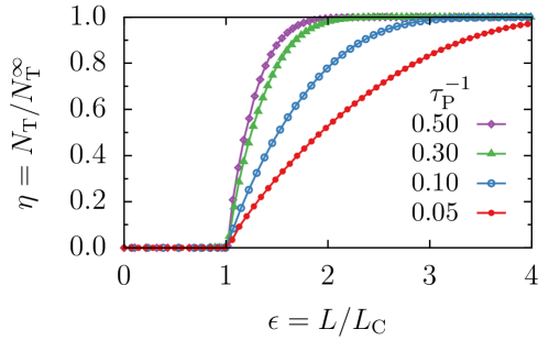
Figure S1: Ratio between the total population for $L$ and for $L\rightarrow\infty$, $\eta$, versus $\epsilon\equiv L/L_{\rm C}$ for various $\tau_{\mbox{\tiny{P}}}^{-1}$ as indicated. Other parameters: $D=0.1$, $\gamma=1$, $r_{\rm H}=0.1$, and $r_{\mbox{\tiny{M}}}\rightarrow-\infty$. The habitat is symmetric, i.e., $x_{\rm R}=-x_{\rm L}$.

References

- Alharbi and Petrovskii, (2016) Alharbi, W. G. and Petrovskii, S. V. (2016). The Impact of Fragmented Habitat’s Size and Shape on Populations with Allee Effect. Mathematical Modelling of Natural Phenomena, 11(4):5–15.
- Arfken and Weber, (1999) Arfken, G. B. and Weber, H. J. (1999). Mathematical methods for physicists.
- Ballard et al., (2004) Ballard, M., Kenkre, V. M., and Kuperman, M. N. (2004). Periodically varying externally imposed environmental effects on population dynamics. Physical Review E, 70(3):7.
- Belgacem and Cosner, (1995) Belgacem, F. and Cosner, C. (1995). The effects of dispersal along environmental gradients on the dynamics of populations in heterogeneous environment. Canad. Appl. Math. Quart, 3(4):379–397.
- Cantrell and Cosner, (1991) Cantrell, R. S. and Cosner, C. (1991). Diffusive Logistic Equations with Indefinite Weights: Population Models in Disrupted Environments II. SIAM Journal on Mathematical Analysis, 22(4):1043–1064.
- Cantrell and Cosner, (1999) Cantrell, R. S. and Cosner, C. (1999). Diffusion models for population dynamics incorporating individual behavior at boundaries: Applications to refuge design. Theoretical Population Biology, 55(2):189–207.
- Cantrell and Cosner, (2001) Cantrell, R. S. and Cosner, C. (2001). Spatial heterogeneity and critical patch size: Area effects via diffusion in closed environments. Journal of Theoretical Biology, 209(2):161–171.
- Cantrell et al., (2006) Cantrell, R. S., Cosner, C., and Lou, Y. (2006). Movement toward better environments and the evolution of rapid diffusion. Mathematical biosciences, 204(2):199–214.
- (9) Channell, R. and Lomolino, M. V. (2000a). Dynamic biogeography and conservation of endangered species. Nature, 403(6765):84–86.
- (10) Channell, R. and Lomolino, M. V. (2000b). Trajectories to extinction: Spatial dynamics of the contraction of geographical ranges. Journal of Biogeography, 27(1):169–179.
- Colombo and Anteneodo, (2018) Colombo, E. and Anteneodo, C. (2018). Nonlinear population dynamics in a bounded habitat. Journal of Theoretical Biology, 446:11–18.
- Colombo and Anteneodo, (2016) Colombo, E. H. and Anteneodo, C. (2016). Population dynamics in an intermittent refuge. Physical Review E, 94(4):1–7.
- Cronin et al., (2020) Cronin, J. T., Fonseka, N., Goddard, J., Leonard, J., and Shivaji, R. (2020). Modeling the effects of density dependent emigration, weak allee effects, and matrix hostility on patch-level population persistence. Mathematical Biosciences and Engineering, 17(2):1718.
- Cronin et al., (2019) Cronin, J. T., Goddard, J., and Shivaji, R. (2019). Effects of patch–matrix composition and individual movement response on population persistence at the patch level. Bulletin of Mathematical Biology, 81:3933–3975.
- Dannemann et al., (2018) Dannemann, T., Boyer, D., and Miramontes, O. (2018). Lévy flight movements prevent extinctions and maximize population abundances in fragile Lotka–Volterra systems. Proceedings of the National Academy of Sciences, 115(15):3794–3799.
- Dos Santos et al., (2020) Dos Santos, M., Dornelas, V., Colombo, E., and Anteneodo, C. (2020). Critical patch size reduction by heterogeneous diffusion. Physical Review E, 102(4):042139.
- Dunn and Gipson, (1977) Dunn, J. E. and Gipson, P. S. (1977). Analysis of Radio Telemetry Data in Studies of Home Range. Biometrics, 33(1):85.
- Fagan et al., (1999) Fagan, W. F., Cantrell, R. S., and Cosner, C. (1999). How habitat edges change species interactions. American Naturalist, 153(2):165–182.
- Fagan et al., (2009) Fagan, W. F., Cantrell, R. S., Cosner, C., and Ramakrishnan, S. (2009). Interspecific variation in critical patch size and gap-crossing ability as determinants of geographic range size distributions. The American Naturalist, 173(3):363–375.
- Fagan et al., (2007) Fagan, W. F., Lutscher, F., and Schneider, K. (2007). Population and community consequences of spatial subsidies derived from central-place foraging. The American Naturalist, 170(6):902–915.
- Ferraz et al., (2003) Ferraz, G., Russell, G. J., Stouffer, P. C., Bierregaard Jr, R. O., Pimm, S. L., and Lovejoy, T. E. (2003). Rates of species loss from amazonian forest fragments. Proceedings of the National Academy of Sciences, 100(24):14069–14073.
- Franklin et al., (2002) Franklin, A. B., Noon, B. R., and George, T. L. (2002). What is habitat fragmentation? Studies in avian biology, 25:20–29.
- Gaston et al., (2002) Gaston, K. J., Pressey, R. L., and Margules, C. R. (2002). Persistence and vulnerability: Retaining biodiversity in the landscape and in protected areas. Journal of Biosciences, 27(4):361–384.
- Gerber et al., (2003) Gerber, L. R., Botsford, L. W., Hastings, A., Possingham, H. P., Gaines, S. D., Palumbi, S. R., and Andelman, S. (2003). Population models for marine reserve design: A retrospective and prospective synthesis. Ecological Applications, 13(sp1):47–64.
- Hastings, (1983) Hastings, A. (1983). Can spatial variation alone lead to selection for dispersal? Theoretical Population Biology, 24(3):244–251.
- Holmes et al., (1994) Holmes, E. E., Lewis, M. A., Banks, J. E., and Veit, R. R. (1994). Partial differential equations in ecology: Spatial interactions and population dynamics. Ecology, 75(1):17–29.
- Ibagon et al., (2022) Ibagon, I., Furlan, A., and Dickman, R. (2022). Reducing species extinction by connecting fragmented habitats: Insights from the contact process. Physica A: Statistical Mechanics and its Applications, 603:127614.
- Jeltsch et al., (2013) Jeltsch, F., Bonte, D., Pe’er, G., Reineking, B., Leimgruber, P., Balkenhol, N., Schröder, B., Buchmann, C. M., Mueller, T., Blaum, N., et al. (2013). Integrating movement ecology with biodiversity research-exploring new avenues to address spatiotemporal biodiversity dynamics. Movement Ecology, 1(1):1–13.
- Kapfer et al., (2010) Kapfer, J., Pekar, C., Reineke, D., Coggins, J., and Hay, R. (2010). Modeling the relationship between habitat preferences and home-range size: a case study on a large mobile colubrid snake from north america. Journal of Zoology, 282(1):13–20.
- Kenkre and Kumar, (2008) Kenkre, V. M. and Kumar, N. (2008). Nonlinearity in bacterial population dynamics: Proposal for experiments for the observation of abrupt transitions in patches. Proceedings of the National Academy of Sciences of the United States of America, 105(48):18752–18757.
- Kierstead and Slobodkin, (1953) Kierstead, H. and Slobodkin, L. B. (1953). The size of water masses containing plankton blooms. J. mar. Res, 12(1):141–147.
- Krams et al., (2021) Krams, R., Krama, T., Brūmelis, G., Elferts, D., Strode, L., Dauškane, I., Luoto, S., Šmits, A., and Krams, I. A. (2021). Ecological traps: evidence of a fitness cost in a cavity-nesting bird. Oecologia, 196(3):735–745.
- Lamb et al., (2017) Lamb, C. T., Mowat, G., McLellan, B. N., Nielsen, S. E., and Boutin, S. (2017). Forbidden fruit: human settlement and abundant fruit create an ecological trap for an apex omnivore. Journal of Animal Ecology, 86(1):55–65.
- Lin et al., (2004) Lin, A. L., Mann, B. A., Torres-Oviedo, G., Lincoln, B., Käs, J., and Swinney, H. L. (2004). Localization and extinction of bacterial populations under inhomogeneous growth conditions. Biophysical Journal, 87(1):75–80.
- Lord and Norton, (1990) Lord, J. M. and Norton, D. A. (1990). Scale and the spatial concept of fragmentation. Conservation Biology, 4(2):197–202.
- Ludwig et al., (1979) Ludwig, D., Aronson, D., and Weinberger, H. (1979). Spatial patterning of the spruce budworm. Journal of Mathematical Biology, 8(3):217–258.
- Maciel and Lutscher, (2013) Maciel, G. A. and Lutscher, F. (2013). How individual movement response to habitat edges affects population persistence and spatial spread. The American Naturalist, 182(1):42–52.
- Martinez-Garcia et al., (2020) Martinez-Garcia, R., Fleming, C. H., Seppelt, R., Fagan, W. F., and Calabrese, J. M. (2020). How range residency and long-range perception change encounter rates. Journal of theoretical biology, 498:110267.
- Mueller et al., (2008) Mueller, T., Olson, K. A., Fuller, T. K., Schaller, G. B., Murray, M. G., and Leimgruber, P. (2008). In search of forage: predicting dynamic habitats of mongolian gazelles using satellite-based estimates of vegetation productivity. Journal of Applied Ecology, 45(2):649–658.
- Nathan et al., (2008) Nathan, R., Getz, W. M., Revilla, E., Holyoak, M., Kadmon, R., Saltz, D., and Smouse, P. E. (2008). A movement ecology paradigm for unifying organismal movement research. Proceedings of the National Academy of Sciences, 105(49):19052–19059.
- Nauta et al., (2022) Nauta, J., Simoens, P., Khaluf, Y., and Martinez-Garcia, R. (2022). Foraging behavior and patch size distribution jointly determine population dynamics in fragmented landscapes. Journal of The Royal Society Interface, 19:20220103.
- Noonan et al., (2021) Noonan, M. J., Martinez-Garcia, R., Davis, G. H., Crofoot, M. C., Kays, R., Hirsch, B. T., Caillaud, D., Payne, E., Sih, A., Sinn, D. L., et al. (2021). Estimating encounter location distributions from animal tracking data. Methods in Ecology and Evolution, 12(7):1158–1173.
- Noonan et al., (2019) Noonan, M. J., Tucker, M. A., Fleming, C. H., Akre, T. S., Alberts, S. C., Ali, A. H., Altmann, J., Antunes, P. C., Belant, J. L., Beyer, D., Blaum, N., Böhning-Gaese, K., Cullen, L., De Paula, R. C., Dekker, J., Drescher-Lehman, J., Farwig, N., Fichtel, C., Fischer, C., Ford, A. T., Goheen, J. R., Janssen, R., Jeltsch, F., Kauffman, M., Kappeler, P. M., Koch, F., LaPoint, S., Markham, A. C., Medici, E. P., Morato, R. G., Nathan, R., Oliveira-Santos, L. G. R., Olson, K. A., Patterson, B. D., Paviolo, A., Ramalho, E. E., Rösner, S., Schabo, D. G., Selva, N., Sergiel, A., Xavier da Silva, M., Spiegel, O., Thompson, P., Ullmann, W., Ziȩba, F., Zwijacz-Kozica, T., Fagan, W. F., Mueller, T., and Calabrese, J. M. (2019). A comprehensive analysis of autocorrelation and bias in home range estimation. Ecological Monographs, 89(2):e01344.
- Northrup et al., (2012) Northrup, J. M., Pitt, J., Muhly, T. B., Stenhouse, G. B., Musiani, M., and Boyce, M. S. (2012). Vehicle traffic shapes grizzly bear behaviour on a multiple-use landscape. Journal of Applied Ecology, 49(5):1159–1167.
- Pachepsky et al., (2005) Pachepsky, E., Lutscher, F., Nisbet, R. M., and Lewis, M. A. (2005). Persistence, spread and the drift paradox. Theoretical Population Biology, 67(1):61–73.
- Penteriani et al., (2018) Penteriani, V., Delgado, M. D. M., Krofel, M., Jerina, K., Ordiz, A., Dalerum, F., Zarzo-Arias, A., and Bombieri, G. (2018). Evolutionary and ecological traps for brown bears Ursus arctos in human-modified landscapes. Mammal Review, 48(3):180–193.
- Pereira and Daily, (2006) Pereira, H. M. and Daily, G. C. (2006). Modeling biodiversity dynamics in countryside landscapes. Ecology, 87(8):1877–1885.
- Perry, (2005) Perry, N. (2005). Experimental validation of a critical domain size in reaction-diffusion systems with Escherichia coli populations. Journal of the Royal Society Interface, 2(4):379–387.
- Ries and Fagan, (2003) Ries, L. and Fagan, W. F. (2003). Habitat edges as a potential ecological trap for an insect predator. Ecological entomology, 28(5):567–572.
- Ries et al., (2004) Ries, L., Fletcher Jr, R. J., Battin, J., and Sisk, T. D. (2004). Ecological responses to habitat edges: mechanisms, models, and variability explained. Annu. Rev. Ecol. Evol. Syst., 35:491–522.
- (51) Robertson, B. A. and Hutto, R. L. (2006a). A framework for understanding ecological traps and an evaluation of existing evidence. Ecology, 87(5):1075–1085.
- (52) Robertson, B. A. and Hutto, R. L. (2006b). A framework for understanding ecological traps and an evaluation of existing evidence. Ecology, 87(5):1075–1085.
- Ryabov and Blasius, (2008) Ryabov, A. B. and Blasius, B. (2008). Population growth and persistence in a heterogeneous environment: the role of diffusion and advection. Mathematical Modelling of Natural Phenomena, 3(3):42–86.
- Schlaepfer et al., (2002) Schlaepfer, M. A., Runge, M. C., and Sherman, P. W. (2002). Ecological and evolutionary traps. Trends in ecology & evolution, 17(10):474–480.
- Skellam, (1951) Skellam, J. (1951). Random Dispersal in Theoretical Populations. Biometrika, 38(1):196–218.
- Speirs and Gurney, (2001) Speirs, D. C. and Gurney, W. S. (2001). Population persistence in rivers and estuaries. Ecology, 82(5):1219–1237.
- Turner, (1996) Turner, I. M. (1996). Species loss in fragments of tropical rain forest: a review of the evidence. Journal of applied Ecology, pages 200–209.
- Van Moorter et al., (2016) Van Moorter, B., Rolandsen, C. M., Basille, M., and Gaillard, J.-M. (2016). Movement is the glue connecting home ranges and habitat selection. Journal of Animal Ecology, 85(1):21–31.
- Vergni et al., (2012) Vergni, D., Iannaccone, S., Berti, S., and Cencini, M. (2012). Invasions in heterogeneous habitats in the presence of advection. Journal of Theoretical Biology, 301:141–152.
- Weldon and Haddad, (2005) Weldon, A. J. and Haddad, N. M. (2005). The effects of patch shape on indigo buntings: evidence for an ecological trap. Ecology, 86(6):1422–1431.
- Zhou and Fagan, (2017) Zhou, Y. and Fagan, W. F. (2017). A discrete-time model for population persistence in habitats with time-varying sizes. Journal of Mathematical Biology, 75:649–704.