Upper Limit on Correlated Current Variations in the Crab Pulsar

Abstract

The high energy emission of rotation powered pulsars is supposed to be produced in "gaps" in the pulsar magnetosphere where charges are accelerated and currents are produced. The rest of the magnetosphere is supposed to be mostly a "force-free" plasma without any currents. Two important currents are the main current that flows away from the pulsar, that produces the observed radiation, and the current that returns to the pulsar to maintain charge neutrality. This work attempts to study the return current in the Crab pulsar using the soft X-ray data from the NICER observatory. It is assumed that the two currents vary as a function of time. This would modulate the electric fields in the "gaps", which would affect the observed X-ray flux. These flux variations will show up only in the on-pulse phases, while those caused by the Crab Nebula, instrumental effects, etc. will be present in the off-pulse phases also. This work obtains the correlation coefficient of the flux variations in the two peaks of the Crab pulsar, after removing the off-pulse flux variations. No correlation was observed; its error of $0.000012$ sets an upper limit of $0.036\%$ on the rms variation of correlated X-ray flux in the Crab pulsar. Reasons exist for the return current variations to be correlated, while the main current variations are probably uncorrelated. So the above number is considered an upper limit on correlated return current variations, which may be an important constraint for pulsar magnetospheric structure.

1 Introduction

Rotation powered pulsars (RPPs) have intense magnetic fields whose rotation causes intense electric fields outside the pulsar. These pull out electrons and ions from the surface of the pulsar which are then accelerated and produce electron-positron pairs. These pairs are themselves accelerated and produce further pairs. Eventually this cascade leads to the outside of the pulsar being filled with a plasma of electrons, positrons and ions co-rotating with the pulsar – this is known as the magnetosphere. For original contributions to this subject see Goldreich & Julian (1969), Ostriker, & Gunn (1969), Sturrock (1971), Ruderman & Sutherland (1975), Arons & Scharlemann (1979), Arons (1983) and Cheng et al. (1986).

Setting aside pair production for a moment, consider what happens when a current of, say, electrons leaves the pulsar. If no other physics intervenes, then a positive charge builds up on the pulsar as a function of time. This would reduce the accelerating electric field and eventually inhibit the outward electron current. The pulsar may end up as a charged and magnetized globe rotating at its period, but not producing the high energy X-rays and $\gamma$-rays that are emitted by the Crab pulsar. This would be an inert electrosphere (Arons, 2009; Spitkovsky, 2011). Clearly pair production intervenes – the accelerated charges emit curvature or synchrotron or inverse Compton photons of high energy, which form the observed radiation. These photons also produce electron-positron pairs in the strong magnetic field of the pulsar. The electrons of the pairs are accelerated in the same direction as the original current, i.e., away from the pulsar, while the positrons are accelerated in the reverse direction, and can reach the pulsar through a region of "force-free" plasma. But this can not be the return current – it has the wrong sign of charge. Therefore a proper return current is a vital component of the pulsar high energy emission mechanism. See Contopoulos et al. (1999), Cheng (2011), Hirotani (2011), Spitkovsky (2011), Arons (2011), Petri (2011) and Contopoulos et al. (2019) for details of the pulsar magnetosphere and the two currents and their relation to the high energy emission mechanism. To the best of my knowledge the return current was first discussed seriously by Arons & Scharlemann (1979).

A brief summary of the essential features of the two currents is given below. It is an observer’s perspective of the essential features of the currents in a RPP, Several theoretical details are unimportant for the current purpose and are therefore ignored (see Cerutti et al. (2016) and Philippov et al. (2020) for illustration).

1.1 The main and return currents in a RPP

Figure 1 (a) shows a cartoon of the pulsar magnetosphere and its various "gaps". It is a two dimensional projection of a three dimensional object. The RPP is defined by its rotation axis $\Omega$ and magnetic dipole axis $\mu$. The magnetosphere is divided into open and closed magnetic field line regions; the field line labeled "last closed field line" defines the boundary between the two. A charge in the closed field line region can not leave the magnetosphere. The rest of the magnetosphere shown consists of open filed line region in which currents can leave and return to the pulsar.

In the open field line region there are three gaps. The polar cap gap lies just above the surface of the pulsar; it was the earliest gap proposed and is currently believed to be the source of the radio radiation of the RPP. It was found unsuitable for the high energy emission because of high magnetic opacity for photons near the surface of the pulsar. So the outer gap was proposed; it extends from a so called null surface at one end to the light cylinder at the other end, both shown as dotted lines in Fig. 1 (a), and has a thickness much smaller than its length. Its lower boundary is quite close to the last closed field line; this is the green area in the figure.

Between the lower boundary of the outer gap and the last closed field line lies the slot gap, a relatively thin gap shown in orange color in the figure. It extends right from the surface of the RPP to the light cylinder.

Now, the main current from the pulsar originates in these gaps and flows away from the pulsar; the charge carried away by this current depends upon whether the angle between $\Omega$ and $\mu$ is acute or obtuse. It is not clear whether all three gaps can operate simultaneously in the same RPP (polar cap gap and outer gap are believed to be mutually exclusive), but at least one of them is active. See Harding & Grenier (2011), Harding (2022) and references therein for details about these gaps.

The return current reaches the RPP through a very narrow bundle of magnetic field lines along the last closed field line; this would be below the slot gap and probably almost coincides with what is known as the separatrix layer, which is like a narrow slot gap that extends beyond the light cylinder. For details of the return current please refer Arons (2011) and particularly its Fig. $5$, and Fig $15.2$ of Arons (2009), and figures $1$ and $2$ of Contopoulos et al. (2019).

The structure of both currents is a strong function of the angle $\alpha$ between the the rotation axis $\Omega$ and the magnetic axis $\mu$.

1.2 Some properties of the main current

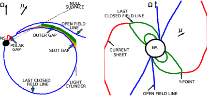
Figure 1: (a) Left panel: Cartoon of Fig. $1$ of Hirotani (2011). (b) Right panel: Cartoon of Fig. $2$ of Spitkovsky (2006). These cartoons are intended only for convenience. For any scientific details the original figures must be referred to. NS is the neutron star (RPP); it is not to scale with respect to the radius of the light cylinder. $\Omega$ and $\mu$ are its rotation and magnetic dipole axes.

The properties of the main current obviously depend upon the gap involved. For the polar cap gap early research postulated periodic build up and breakdown of the gap on timescales of micro seconds (Ruderman & Sutherland, 1975), leading to a current that sparks on time scales of micro seconds. This was revised later to a space charge limited quasi steady state current due to the work function of iron ions on the surface of the neutron star. The main current in all gaps depends upon the so called "favorably curved magnetic field lines" (see Cheng (2011) and references therein). In all gaps pair production reduces the effective electric field due to screening by the pairs – then one has a space charge limited flow. In the outer gap the current is quite low in the accelerating region but much larger in the screening region (Cheng, 2011). The magnitude of the main current depends upon the gap thickness. So high-altitude slot gaps can not produce sufficient high energy flux due to their being thin (Hirotani, 2011).

1.3 The return current and the current sheet

The last closed field line has been depicted as almost a circle in Fig. 1 (a). Modern particle-in-cell simulations show it to be actually that depicted in Fig. 1 (b). It develops a sharp projection at the point where it just touches the light cylinder; this is known as the "Y-point". Here it also connects with the so called "current sheet", shown in red in the figure (strictly the Y-point does not necessarily have to touch the light cylinder (Spitkovsky, 2011)). Most of the return current originates far away from the RPP and flows towards it in the current sheet. At the Y-point the return current splits into two streams along the last closed field line, each proceeding to one of the two magnetic poles of the RPP. Although the current sheet has been represented by a red curve of uniform width in Fig. 1 (b), it is thickest at the Y-point and reduces in thickness further away from the RPP.

1.4 Some properties of the return current

The above is a two dimensional projection of a three dimensional object, the projection being in the plane containing the vectors $\Omega$ and $\mu$. So the current sheet is actually a current ring or a current torus, and the Y-point is actually a Y-volume since it has finite extension in all three dimensions, and the return current is flowing down the edge of a three dimensional magnetic funnel at the polar caps of the RPP. The nature of the current sheet and the return current it provides depend upon the angle $\alpha$. The magnitude of the return current decreases, and its magnetospheric distribution changes dramatically, with $\alpha$ (Spitkovsky, 2011). The return current path is also expected to carry a counter-streaming current (Arons, 2011; Contopoulos et al., 2019). In this work we are concerned with the net return current which is the sum of all counter-streaming currents, if at all they exist.

It is now suspected that the high energy emission from RPPs originates due to reconnection in the current sheet, presumably at the Y-point. See Spitkovsky (2011), Arons (2011) and Petri (2011) for details.

1.5 The philosophy of this analysis

To begin with, it is assumed that both the main and return currents together determine the maximum available electric potential in the gaps, which is related to the X-ray flux emitted by the RPP. The gaps can be thought of as electrical batteries that are charged and discharged by the two currents in a collective manner, implying higher and lower electric potential available for particle acceleration, respectively. However the dynamics of the two currents are likely to be vastly different – the main current is powered by the immense rotational inertia of the pulsar and its intense magnetic field, and depends upon the details of the gaps, the pair production process, and the high energy emission mechanism. On the other hand, the return current begins its journey somewhere far away from the RPP and depends critically upon the details of the current sheet and the pulsar magnetosphere.

Next it is assumed that both currents vary as a function of time. Clearly a steady, unchanging current is not logical, given the highly energetic and almost explosive environment in the pulsar magnetosphere. What is not known is the time scale of such variations. It is assumed here that all possible time scales of variation exist in the currents.

Next, one notes regarding the main current that ($1$) its variations are unlikely to be correlated at the two poles, since the emission at each pole is expected to be independent, and ($2$) the emission at each pole may or may not be correlated across different phases in the folded light curve (FLC) of the RPP, which are equivalent to different regions of emissions in the gaps. On the other hand, variations imposed upon the return current beyond the Y-point are certainly correlated not only at the two poles but also at all phases in the FLC, although one can not rule out de-correlating variations being imposed on the return current between the Y-point and the surface of the RPP.

The purpose of this work is to study correlated flux variations if any in the Crab pulsar. The basic premise of this work is that the return current variations (beyond the Y-point) should be imprinted on the X-ray flux of the RPP, while the main current variations may or may not be imprinted. Further, these variations will exist in the pulsar flux, and not in that from the nebula. So the technique used here is to divide the FLC of the Crab pulsar into three regions of phase – the main peak and the second peak (forming the so called on-pulse region), and the off-pulse region. The nebular flux and instrumental effects will exist at all phases while the current variations are expected only in the on-pulse. The idea is to correlate the X-ray flux in the two peaks of the Crab pulsar, after estimating the nebular flux variations and/or instrumental effects from the off-pulse phases and removing them from the on-pulse phases. At best this number will be determined only by the return current variations; however one can not rule out correlated main current variations altogether.

Incidentally, variations of currents in a RPP can also manifest as variations of electromagnetic torque on the RPP, leading to fluctuations in its rotation period. This is commonly known as timing noise. This work addresses a particular component of it, that which is correlated across the FLC of the RPP. As mentioned earlier in this section, only the return current may display such a correlation. Given the possibility of de-correlating effects before the Y-point, it is possible that the correlated return current variations may be a very small fraction of the total current variations in the RPP. In such a situation the correlated return current variations may not leave a measurable imprint on the timing noise of a RPP.

In footnote $6$ on page $387$ Arons (2009) states that observational study of pulsar currents has been an untouched subject. This work attempts to redress this issue.

2 Observations and analysis

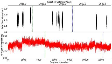
Figure 2: (a) Top panel: Long time light curve (LTLC) of the Crab pulsar from NICER data in the energy range $1-10$ keV with a bin size of $10$ s, using the $27$ observations specified in Vivekanand (2021); the abscissa is exactly the same as in its Fig. $1$; the ordinate is in units of thousand photons per second. (b) Bottom panel: LTLC using the same data but with a bin size of $300$ periods, which is $\approx 10.125$ s; the abscissa is sequence number of the bins while the ordinate is in photons per period. The green and blue dashed lines mark the same epochs respectively in both panels.

The details of the NICER observations used here and their preliminary analysis are given in Vivekanand (2020, 2021).

The top panel of Fig. 2 is the long time light curve (LTLC) of the Crab pulsar with a bin size of $10$ s in the energy range $1$ to $10$ keV. This consists of $137161$ s of data equivalent to $\approx 4.06$ million periods. It is similar to Fig. $1$ of Vivekanand (2021) except that a small amount of initial data is not included for reasons stated there, and the energy range is different. The bottom panel of Fig. 2 is the same data with a bin size of $300$ periods which is approximately $10.125$ s. The binning is in number of periods because this analysis depends upon the phase in the FLC, so the period is the natural unit for binning. It also eliminates the error introduced by fractional periods of data at the beginning and the end of a time bin. By plotting the data in terms of the sequence number of the bins one eliminates the large gaps in the epoch in the top panel, leading to a better appreciation of the variability of the X-ray flux of the Crab pulsar. The green and blue dashed lines in the top panel represent the epochs $2018.25$ and $2019.25$ respectively. The corresponding lines in the bottom panel mark the partitioning of the data in terms of these epochs. Thus the sequence numbers in the bottom panel just before and just after the green dashed line correspond to the time bins just before and just after the green dashed line in the top panel. The same is true for the blue dashed lined in both panels. However the correspondence is approximate since the bins in both panels are slightly different in terms of time. Further, the period bins in the bottom panel of Fig. 2 are slightly larger in terms of time towards later epochs since the period of the Crab pulsar increases with epoch.

The bottom panel of Fig. 2 was obtained by first searching for a new period at the start of each good time interval (GTI), then accumulating photon counts over $300$ contiguous periods for each bin. The incomplete bin at the end of the GTI is discarded. The mean and rms of the counts are $253.79$ and $1.79$ respectively; the rms is a fraction $1.79/253.79=0.00705$ of the mean or $\approx 0.71\%$. As shown later on this variation of X-ray flux is present at all phases in the FLC. Therefore this must be either due to the Crab nebula or due to instrumental effects such as pointing variations of NICER. Now, this number is consistent with the $1^{\prime}$ pointing errors of NICER producing $2\%-4\%$ flux variations. These variations have to be removed from the data before estimating those that exist only in the on-pulse phases.

The analysis begins by defining three phase ranges in the period of the Crab pulsar – first peak, second peak and off-pulse, labeled P1, P2 and P3 respectively, with respect to Fig. $1$ of Vivekanand (2022). The three phase ranges were finalized after some experimentation as $0.1015625$ to $0.40625$, $0.40625$ to $0.796875$, and the rest of the phase range, respectively, the specific numbers being chosen so as to correspond to integer multiples of $1/128$ phase, and also to maximize the off-pulse phase range without compromising on the on-pulse phase range. The final results of this work are not sensitive to the exact choice of the above phase range limiters. P1 and P2 together form the on-pulse phase range while P3 is the off-pulse.

Throughout this work it will be assumed that component P3 contains no pulsar flux, in spite of Tennant et al. (2001) discovering off-pulse non-thermal X-ray emission from the Crab pulsar at much softer X-ray energies, because their Fig. $1$ shows that this flux is about two orders of magnitude smaller than the flux at the first peak of the Crab pulsar.

The next section implements the cross-correlation analysis upon the data of P1, P2 and P3 to reproduce the $\approx 0.71\%$ flux variation in all three components. This is to validate our analysis method. In the following section these variations are estimated in the P3 component and removed from all three components. Cross-correlation of the modified P1 with the modified P2 should give us the correlated variations that exist only in the on-pulse, which will be attributed to current variations in the Crab pulsar. Correspondingly cross-correlation of the modified P1 and P2 with the modified P3 should result in almost zero correlation.

3 Analysis of raw data

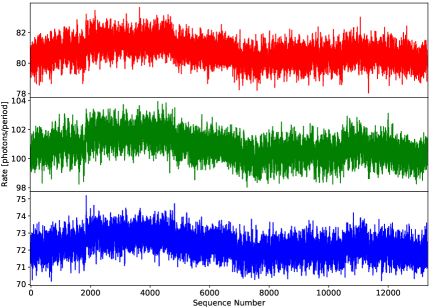
Figure 3: Same as the bottom panel of Fig. 2 but for each of the components P1, P2 and P3 of the FLC (top, middle and bottom panels respectively).

Figure 3 is the same as the bottom panel of Fig. 2 but for each of the components P1, P2 and P3 of the FLC; the sum of these three rates is exactly equal to the corresponding rate in the bottom panel of Fig. 2. The flux variation of Fig. 2 exists in all three components of the FLC. It is know from Fig. 2 that the fractional flux variation is $\approx 0.71\%$ of the mean flux. This will now be derived by cross correlating the fluxes in the three components, so as to validate the procedure for the next section.

In Fig. 3 the X-ray flux data has been averaged over $300$ periods for convenience of visualization and plotting. However the cross correlation of the data must be estimated using the raw (un-averaged) data, since averaging the data before cross correlating it biases it to larger values. This is because averaging the data decreases the denominator while maintaining approximately the same numerator in the formula for cross correlation (Appendix A). In a larger context this problem is related to what is known as “ecological fallacy" in which correlation of aggregate data is used to interpret possible correlation among individual data, which can be misleading. In our case therefore the cross correlation must be done with the data of count rate per a single period.

Table 1 lists the estimated cross correlation $R$ between pairs of components in the FLC of the Crab pulsar, along with the derived fractional rms variation $\sigma_{c}$ of the correlated X-ray flux (see Appendix A, which also explains the error on the cross correlation). The $\sigma_{c}$ values in Table 1 and the upper and lower limits of errors have not been rounded off to bring out the fact that a uniform error of $0.0004$ or $0.0005$ is a good enough approximation instead of the upper and lower limits. Results for the three $\sigma_{c}$ values are $0.70(4)\%$, $0.66(5)\%$ and $0.69(4)\%$, which are consistent with each other. Their weighted mean is $0.69(2)\%$ which is consistent with the value of $\approx 0.71\%$ estimated in the previous section. Our analysis is therefore validated for use in the following section.

Appendix B discusses the so called “ecological fallacy" and the variation of the cross correlation $R$ for data averaged over $M$ samples.

Table 1: Cross correlation $R$ of X-ray flux data binned at $1$ (one) period between pairs of phase components P1, P2 and P3. $\sigma_{c}$ is the resulting rms flux variation of the correlated component as a fraction of the mean counts. The error in the last digit in $R$ is given in brackets. See Appendix A for computational details.

Component pairs	$R$ (Correlation)	$\sigma_{c}$ (Fractional rms)
(P1, P2)	$R_{12}=0.0044(5)$	$0.00701_{-0.00041}^{+0.00039}$
(P1, P3)	$R_{13}=0.0033(5)$	$0.00656_{-0.00052}^{+0.00048}$
(P2, P3)	$R_{23}=0.0041(5)$	$0.00691_{-0.00044}^{+0.00041}$

4 Analysis of filtered data

In this section one will first estimate the smooth version of the flux in component P3 (bottom panel of Fig. 3), and use that to remove the corresponding flux variation in components P1 and P2 before cross correlation. There are several algorithms for smoothing data; see any graduate school level text book on filtering data in the subject of digital signal processing. To ensure that the results of this section are independent of the smoothing algorithm, three filters were used: the Savitzky-Golay filter, the moving average filter, and the Wiener filter.

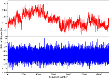
Figure 4: (a) Top panel: Data of phase component P3 (bottom panel of Fig. 3) filtered by a Savitzky-Golay algorithm using a window width of $30$ samples and a polynomial of degree $2$. (b) Bottom panel: Difference between the original and filtered data.

All three filters have one common parameter known as the the smoothing window $N_{sw}$ in units of data samples. In addition, the Savitzky-Golay filter uses a polynomial of degree L, which is usually low ($\approx 2-3$). It smooths the data by representing it in each segment of $N_{sw}$ samples by a polynomial with L different coefficients. The moving average filter smooths the data by representing each data point by the average of $N_{sw}$ adjacent samples. The Wiener filter assumes that it knows the signal and noise power spectra, and applies low weightage to data segments (of width $N_{sw}$ samples) where the signal to noise ratio is low.

Fig. 4 shows an example of smoothing the data using the Savitzky-Golay filter with $N_{sw}=30$ and $L=2$. The top panel displays the filtered data while the bottom panel displays the difference between the original and filtered data, which looks like white noise, as it should. Once again it is mentioned that although Fig. 4 shows X-ray flux data averaged over $300$ periods, the cross correlation is done using un-averaged data. Moreover, the cross correlation coefficient $R$ now depends upon the filter window width $N_{sw}$. The detail of this analysis are given in Appendix C and the results are given in Table 2.

Table 2: Cross correlation $R$ (in units of $10^{-5}$) of flux binned at $1$ (one) period between pairs of phase components P1, P2 and P3, after estimating the flux trend in P3 and removing it from all three components. Three filters were used for estimating the trend in P3 – Savitsky-Golay (SG), moving average (MA) and Wiener (WI). See Appendix C for computational details.

	Filter
$R(\times 10^{5})$	SG	MA	WI
$R_{12}$	$1.2\pm 1.2$	$0.40\pm 0.59$	$0.40\pm 0.59$
$R_{13}$	$0.10\pm 0.12$	$-0.30\pm 0.19$	$-0.30\pm 0.24$
$R_{23}$	$-0.2\pm 0.19$	$0.20\pm 0.12$	$0.20\pm 0.12$

Table 2 gives the cross correlation coefficient $R$ for all three pairs of phase components for all three filters. Each $R$ in Table 2 has been estimated with reference to a “calibration” $R$ that should ideally be zero; this is account for any uncertainty in removing the smooth version of the flux of component P3 (see Appendix C for details of the analysis). All $R$ are either smaller than or comparable to their errors, so they are essentially zero. This is because they are the difference between two numbers that have very similar values (Appendix C). Since no significant cross correlation has been estimated, the largest error on the cross correlations in Table 2 ($1.2\times 10^{-5}$) sets the upper limit for $\sigma_{c}$, which turn out to be $0.036\%$. Thus the correlated X-ray flux in the phase components P1 and P2 of the Crab pulsar is less than this value. In principle this includes variations from both the main and the return currents. Therefore this number is the upper limit on the correlated variation of the return current in the Crab pulsar.

5 Correlation of X-ray flux from the two poles

In section $1.5$ it was argued that the return current variations beyond the Y-point are correlated at the two poles. In this section attempt will be made to test this hypothesis although it was acknowledged in section $1.5$ that variations imposed upon the return current before the Y-point may lead to de-correlation.

The observed X-ray radiation from a RPP is emitted in the gaps in the pulsar magnetosphere. Within the gaps the radiation is emitted with its momentum vector tangent to the local magnetic field line; this radiation is observed whenever the line of sight to the RPP is parallel to this tangent. Now in Fig. 1 (a) only one half of the magnetosphere is drawn – a symmetrical gap system exists at the other magnetic pole. Therefore it is possible that one may observe radiation from both poles depending upon the angle $\alpha$ between the rotation and magnetic axis, and the angle between the rotation axis and the line of sight. It is easier to visualize this in Fig. 1 (b) where magnetic field lines are drawn at both poles. Now, there will be a delay in the arrival time of radiation from the pole farther away from the observer, which would be typically $\approx$ a light cylinder distance farther away from the closer pole. This distance would take the radiation about $P/(2\pi)$ s of travel time where $P$ is the rotation period of the RPP; this number may be a bit larger depending upon the above mentioned two angles. So the Crab pulsar’s X-ray flux may have correlated flux variations with a delay of a fraction of the period, which would translate to an equivalent phase delay in the FLC.

This effect should be studied by using phase bins of much higher resolution than those of the previous section. This would naturally decrease the number of photons in these bins making the estimation of cross correlation more difficult. In this section the FLC was divided into $128$ phase bins; the number of photons per phase bin (per period) reduced to typically $1-2$ photons, which is very small. The attempt was to cross correlate the data of the bin at the first peak of the FLC of the Crab pulsar, with all other bins except those in the off-pulse. Any correlated variations from the two poles should show up as a secondary peak of cross correlation about $1/(2\pi)$ phase away from the first peak. As in the previous section, the variations in the off-pulse have to be removed before correlating.

Table 3: Cross correlation $R$ (in units of $10^{-5}$) of flux binned at $1$ (one) period at phase bins $17$ and $69$ in the FLC with a resolution of $128$ bins; off-pulse (same P3 of the previous section) flux trend was removed from all three components. The Savitsky-Golay (SG) filter was used for trend estimation.

	Filter
$R(\times 10^{5})$	SG
$R_{17,69}$	$0.4\pm 0.1$
$R_{17,P3}$	$-5.4\pm 0.2$
$R_{69,P3}$	$1.6\pm 0.3$

The analysis of the previous section was repeated using the Savitzky-Golay filter, and the results are presented in Table 3 which shows, for the purpose of illustration, the result of correlating the data at phase bin number $17$ (at the first peak) and at bin number $69$ (at the second peak), using the same off-pulse phase range as earlier (P3). Although the correlations in the three rows are larger than their formal errors, the correlations of data at bin numbers $17$ and $69$ with the data of P3 (bottom two rows of Table 3) are much larger than the correlation of data of the two bins (top row of Table 3). This implies that the data trend of P3 has not been removed completely from the data of bins $17$ and $69$. Clearly the correlations are consistent with no correlation, probably because the number of photons per phase bin are too small for this exercise.

6 Discussion

The summary of this work is that it attempts to estimate correlated soft X-ray flux variations in the on-pulse phases of the Crab pulsar, after removing flux variations due to the Crab nebula and/or instrumental effects. No correlation was detected; the measurement error on the correlation sets an upper limit of $0.036\%$ on the rms variation of correlated flux. In principle this could be due to both the main as well as the return currents; therefore the above number is an upper limit on the correlated variations of the return current in the Crab pulsar.

A few caveats will be stated before proceeding further. In this work it has been assumed that variations of the return current beyond the Y-point are carried back to the star. However Arons (2009) cautions that it is yet to be demonstrated whether this is possible. Next, the return current has details that have been ignored in this work; for example $20\%$ of it flows to the pulsar along a different but close path; see Arons (2009) for details.

In order to study the return current variations one should be able to decouple them from the main current variations. This depends upon the time scales on which the two are coupled, but currently this is not known. For illustration consider an extreme example – let the source of the return current be at half distance to the Crab nebula, which has a size of radius $\approx 2^{\prime}$ in the sky. Assuming that the Crab pulsar is at a distance of $\approx 2000$ parsec, the source of the return current is $\approx 1/60\times\pi/180\times 2000\approx 0.58$ parsec from the pulsar. So any change at the source of the return current will take at least $\approx 1.9$ years to be felt at the pulsar, and a consequent change in the main current will take another $\approx 1.9$ years to be registered back at the source of the return current. Under these circumstances variations in the two currents can be considered to be decoupled and can be discussed separately, even though one does not know their relative strengths. On the other hand, if the above time scale is much shorter then variations in the two currents are closely coupled, and can not be discussed separately; they might form what is known in electronics as a feed back system.

An appropriate example here is a radio receiver with feed back – a strong negative feed back will kill the output, a mild negative feed back will reduce the receiver noise power, a mild positive feed back will convert the receiver into an oscillator, and a strong positive feed back will push the receiver into saturation. The above should be kept in mind while discussing the return current.

One of the direct consequences of variations of the currents is the simultaneous variation in observed emission at all energies. This would require a campaign of multi-wavelength observations with high time resolution and high sensitivity, which are not available. However simultaneous observations at the radio and X-rays are available on three pulsars — PSR B0823+26 (Sobey et al., 2015; Hermsen et al., 2018), PSR B0943+10 (Hermsen et al., 2013; Mereghetti et al., 2016) and PSR B1822-09 (Hermsen et al., 2017). All three pulsars exhibit two main modes of emission – a radio B (bright) mode in which the pulsars are bright in the radio, and a radio Q (quiescent) mode in which they are much weaker. Together these three RPPs make an interesting contradiction which the return current may or may not be able to resolve.

In PSR B0823+26 the X-ray flux in the B mode has a $\approx 20\%$ flux variation which the authors call a new kind of behavior (Hermsen et al., 2018). They speculate that the Q mode is not a true "null" mode – they believe some residual emission exists but being weak it is not observed at earth. They believe the mode changes in this pulsar are entirely different from those in the other two pulsars. They believe that B0823+26 is accreting material from its external environment, either from the interstellar medium, or from an accretion disk.

Now, any accreted material would be eventually ionized and must be funneled to the RPP along the same path as taken by the return current – along other paths the currents are only allowed to leave the pulsar. In such a scenario, the return current can serve the same purpose as the accreted material, which will no longer be needed for the above model. Clearly several details have to be worked out in this scenario – how much extra return current is required, can it be supplied by the current sheet, can the additional return current explain the observed spectral and temporal features as well as the accreted material can, and so on; but this possibility is worth exploring. Arons (2009) mentions that fluctuations of the currents at the light cylinder can probably explain the flickering nature of pulsars, although his context may have been different.

If the return current is varying in PSR B0823+26 as speculated above, then one should also speculate if it is operating similarly in the other two pulsars also; here one encounters some difficulties.

The soft X-ray emission is correlated with the radio emission in B0823+26 – in the B mode both radio and X-rays are observed, while both are not observed in the Q mode. The return current can offer a simple explanation for this – it is larger in the Q mode than in the B mode, so the maximum electric potential available for particle acceleration in the gaps is smaller in the Q mode. Since this affects the basic emission mechanism of the RPP, radiation at all wavelengths can be expected to decrease.

However, the soft X-ray emission is anti-correlated with the radio emission in PSR B0943+10 – the radio emission is weaker in the Q mode while the X-ray emission is weaker in the B mode by a factor of $\approx 2$. Clearly the same return current that can explain the broad band behavior of B0823+26 will fail in the case of B0943+10. One can attempt to salvage the situation by noting that the return current behavior can be different in the two pulsars because B0943+10 is a nearly aligned rotator ($\alpha\approx 0^{\circ}$) while B0823+26 is a nearly orthogonal rotator ($\alpha\approx 90^{\circ}$), and the return current is a strong function of the angle $\alpha$ between the rotation and the magnetic axis. Even then to explain the anti-correlation a new element has to brought in – formation of coherent bunches of particles.

Suppose that in PSR B0943+10 a high return current causes a higher number of coherent bunches of particles; this would imply a higher level of radio emission even though the maximum available electric potential has decreased. But this is not sufficient – one has to come up with a reason why this effect does not operate in PSR B0823+26. Clearly one is reaching the limits of reasonable speculation. This point is further emphasized by the fact that in PSR B1822-09, which is an orthogonal rotator, the radio and X-ray emission are uncorrelated.

To summarize the discussion so far, the return current can explain (in principle) the behavior of PSR B0823+26, but fails to explain the behavior of PSR B0943+10 and PSR B1822-09. See the references above for much greater details in the behavior of these RPPs. It is not clear what causes these behavior, but the return current may be a partial explanation.

So far one focused on what may be called the traditional physics of RPPs, in which the gaps are the sites of pair production as well as emission of observed radiation. Recent research favors the observed radiation to be produced outside the light cylinder. It involves concepts such as the striped wind in which the magnetic polarity is continuously reversed, relativistic beaming effects and so on; it depends upon the inverse Compton scattering process. This model is apparently successful in fitting the observed $\gamma$-ray FLCs of the Geminga and Vela RPPs, as well as the optical polarization data of the Crab pulsar (see Petri (2011) and references therein).

It is possible that in such models the role of the return current is merely to maintain sufficient electrical potential in the gaps for pair production. However in this new scenario particle acceleration can occur in the current sheet near the light cylinder by the method of magnetic reconnection (Kirk et al, 2009; Arons, 2011). In these models the gaps are no longer the only sites of particle acceleration. So in these models maybe the return current has the simplest role – that of ensuring that the pulsar does not end up as an inert electrosphere.

7 Data availability

The data underlying this article are available at the NICER observatory site at HEASARC (NASA).

8 Acknowledgments

I thank Craig Markwardt for discussion on some technical issues such as pointing errors. I thank I. Contopoulos for discussion regarding the return current.

Appendix A Formula for $R$ and $\sigma_{c}$

Let $X_{i},Y_{i}$ ($i=1,...,N$) be N samples of data from two different statistical distributions that have some correlation. Let their mean values be $<X>=\left(\sum_{i}^{N}X_{i}\right)/N$ and $<Y>=\left(\sum_{i}^{N}Y_{i}\right)/N$ and their standard deviations be $\sigma_{X}=\left<\left(X-<X>\right)^{2}\right>$ and $\sigma_{Y}=\left<\left(Y-<Y>\right)^{2}\right>$ respectively. Their cross correlation is defined as

$$R_{XY}=\left<\left(X-<X>\right)\left(Y-<Y>\right)\right>/(\sigma_{X}\sigma_{Y}).$$ (1)

The standard deviation of the correlation coefficient is $(1-R_{XY}^{2})/\sqrt{N}$ (Bowley, 1928). Since the correlation coefficient here is very small compared to $1$, the error on $R_{XY}$ has been estimated as $1/\sqrt{N}$ in column $2$ of Table 1, with $N\approx 4.06$ million.

Now let the two data consist of a correlated signal $c_{i}$ and uncorrelated noise $s_{i}$, both defined as fractions of the mean value, so that

$$\begin{array}[]{ll}X_{i}&=<X>\left(1+c_{i}+s_{Xi}\right)\\ Y_{i}&=<Y>\left(1+c_{i}+s_{Yi}\right).\\ \end{array}$$ (2)

The correlated signal $c_{i}$ is common to both data while the noise in the two data streams are different and therefore uncorrelated, not only among themselves but also with the correlated signal. The statistical properties of the correlated signal are:

$$\begin{array}[]{ll}<c>=0;\sigma_{c}^{2}=\left<\left(c-<c>\right)^{2}\right>=\left<c^{2}\right>\\ <cs_{X}>=<cs_{Y}>=0.\\ \end{array}$$ (3)

The statistical properties of the noise signals are:

$$\begin{array}[]{ll}<s_{X}>=0;\sigma_{sX}=\left<\left(s_{X}-<s_{X}>\right)^{2}\right>=\left<s_{X}^{2}\right>\\ <s_{Y}>=0;\sigma_{sY}=\left<\left(s_{Y}-<s_{Y}>\right)^{2}\right>=\left<s_{Y}^{2}\right>\\ <s_{X}s_{Y}>=0.\\ \end{array}$$ (4)

Now the noise signals obey Poisson statistics so their variance is equal to the mean counts. So the variance of the product $(<X>s_{X})$ is $<X>$, so that

$$\begin{array}[]{ll}<X>^{2}\sigma_{sX}^{2}=<X>\Rightarrow\sigma_{sX}=1/\sqrt{<X>}\\ <Y>^{2}\sigma_{sY}^{2}=<Y>\Rightarrow\sigma_{sY}=1/\sqrt{<Y>}\\ \end{array}$$ (5)

Therefore

$$\begin{array}[]{ll}R_{XY}&=\left<\left(c+s_{X}\right)\left(c+s_{Y}\right)\right>/\left(\sqrt{\sigma_{c}^{2}+\sigma_{sX}^{2}}\sqrt{\sigma_{c}^{2}+\sigma_{sY}^{2}}\right)\\ &=\sigma_{c}^{2}/\left(\sqrt{\sigma_{c}^{2}+\sigma_{sX}^{2}}\sqrt{\sigma_{c}^{2}+\sigma_{sY}^{2}}\right)\\ &=1/\left(\sqrt{1+(\sigma_{sX}/\sigma_{c})^{2}}\sqrt{1+(\sigma_{sY}/\sigma_{c})^{2}}\right)\\ \end{array}$$ (6)

This can be solved for $\sigma_{c}$:

$$\begin{array}[]{ll}R_{XY}^{2}=1/\left[\left(1+(\sigma_{sX}/\sigma_{c})^{2}\right)\left(1+(\sigma_{sY}/\sigma_{c})^{2}\right)\right]\\ \Rightarrow R_{XY}^{2}\left[1+(\sigma_{sX}/\sigma_{c})^{2}+(\sigma_{sY}/\sigma_{c})^{2}+(\sigma_{sX}/\sigma_{c})^{2}(\sigma_{sY}/\sigma_{c})^{2}\right]=1\\ \Rightarrow\left[\sigma_{c}^{4}+\sigma_{c}^{2}(\sigma_{sX}^{2}+\sigma_{sY}^{2})+\sigma_{sX}^{2}\sigma_{sY}^{2}\right]=\sigma_{c}^{4}/R_{XY}^{2}\\ \Rightarrow\sigma_{c}^{4}(1-1/R_{XY}^{2})+\sigma_{c}^{2}(\sigma_{sX}^{2}+\sigma_{sY}^{2})+\sigma_{sX}^{2}\sigma_{sY}^{2}=0\\ \end{array}$$ (7)

This is a quadratic equation in $\sigma_{c}^{2}$ whose solution is:

$$\begin{array}[]{ll}\sigma_{c}^{2}=A\pm B;\\ A=-(\sigma_{sX}^{2}+\sigma_{sY}^{2})/C;\\ B=\left[(\sigma_{sX}^{2}+\sigma_{sY}^{2})^{2}-4(1-1/R_{XY}^{2})\sigma_{sX}^{2}\sigma_{sY}^{2}\right]^{1/2}/C\\ C=2(1-1/R_{XY}^{2}).\\ \end{array}$$ (8)

One of the solutions is negative which is unphysical, so we adopt the positive solution.

Now the mean counts in the P1, P2 and P3 phases in Fig. 3 are $80.7$, $100.8$ and $72.2$ respectively. The corresponding $\sigma_{s1}$, $\sigma_{s2}$ and $\sigma_{s3}$ are $0.1113$, $0.0996$ and $0.1177$ respectively. These are of the order of $0.1$ while the rms of the correlated signal $\sigma_{c}$ is $\approx 0.007$, which is much smaller. Note that all these values are relative to the mean counts in that phase. In this limit the cross correlation simplifies to

$$R_{XY}\approx\sigma_{c}^{2}/\left(\sigma_{sX}\sigma_{sY}\right)$$ (9)

Appendix B “Ecological fallacy"

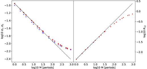
Figure 5: (a) Left panel: Estimated standard deviations of the data in phases P1 (red stars) and P2 (blue pluses) respectively, as a function of the number of periods averaged ($M$). The straight line is the least squares fit to the first $6$ data of P1; the dotted line is its continuation. (b) Right panel: The cross correlation $R_{12}$ of the averaged data as a function of $M$.. The straight line is the least squares fit to the first $6$ data; the dotted line is its continuation.

Consider what happens when the data of Appendix A is averaged before cross correlation, say by $M$ samples. Now one has a new data set $U_{i},V_{i}$ ($i=1,...,N/M$, assuming that $N$ is an integral multiple of $M$), where

$$\begin{array}[]{ll}U_{i}=(\sum_{j=k}^{l}X_{j})/M;V_{i}=(\sum_{j=k}^{l}Y_{j})/M;\\ k=(i-1)\times M+1;l=i\times M.\\ \end{array}$$ (10)

The correlation coefficient $R_{UV}$ will be approximately $R_{XY}\times M$ as long as the time scale of variation of the correlated signal $c$ is much larger than $M$ samples; then the numerator in equation A.1 will not change while the denominator decreases as $1/M$. This is evident in equation A.9.

The left panel of Fig. 5 shows the variation of the estimated standard deviations $\sigma_{1}$ and $\sigma_{2}$ of the data in phases P1 and P2 respectively, as a function of the number of periods averaged ($M$), in a log10-log10 plot. These are the $\sigma_{X}$ and $\sigma_{Y}$ used in equation A.1, and should be equivalent to $\sqrt{\sigma_{c}^{2}+\sigma_{sX}^{2}}$ and $\sqrt{\sigma_{c}^{2}+\sigma_{sY}^{2}}$ respectively. Initially both parameters decrease inversely with $\sqrt{M}$ as expected, then the decrease is slower. A least squares straight line fit to the first six data of each standard deviation yields the results shown in Table 4.

Table 4: Slope and intercept of the straight lines fit in a least squares sense to the logarithm (of base $10$) of $\sigma_{1}$ and $\sigma_{2}$ as a function of logarithm of $M$.

Phase	Slope	Intercept
P1	$-0.4935(9)$	$-0.9545(6)$
P2	$-0.4908(14)$	$-1.0033(9)$

Initially the slopes are very close to the expected value $-0.5$, then the slope reduces in magnitude. Now, the observed value of $\sigma_{1}$ at $M=900$ (the last red point in the left panel of Fig. 5) is $0.0070$ while the value expected on the basis of the straight line is $0.0039$. Since the standard deviations add quadratically, the difference rms is $\sqrt{0.0070^{2}-0.0039^{2}}=0.0058$ which is quite close to the expected value of $\approx 0.0070$. In other words the red stars data is the square root of the quadratic addition of a fixed rms of about $0.0058$ and a variable rms of $\approx 0.1/\sqrt{M}$. Similar results occur for $\sigma_{2}$ in the figure. It is therefore concluded that $\sigma_{1}$ and $\sigma_{2}$ vary as expected in Fig. 5. In the right panel of Fig. 5 $R_{12}$ varies correspondingly. A least squares straight line fit to the first six data give slope $=0.9239(5)$ and intercept $=-2.3458(3)$. Initially the correlation varies almost linearly with $M$ as expected, then varies more slowly. The intercept implies a correlation of $10^{-2.3458}=0.0045$ which is consistent with the $R_{12}$ of Table 1.

Fig. 5 is a check on the basic health of our data.

Appendix C Details of filtering data

Let $g1$, $g2$ and $g3$ be the X-ray fluxes in the three phase components P1, P2 and P3 respectively; each contains $\approx 4.06$ million samples. Let their mean values be $<g1>$, $<g2>$ and $<g3>$. Let $h1$, $h2$ and $h3$ be the smooth versions of $g1$, $g2$ and $g3$ respectively, obtained using a smoothing window of $N_{sw}$ samples and one of the three filtering algorithms. Then two new data are formed as follows:

$$\begin{array}[]{ll}g1^{\prime}=g1-(<g1>/<g3>)h3;&g1^{\prime\prime}=g1-h1\\ g2^{\prime}=g2-(<g2>/<g3>)h3;&g2^{\prime\prime}=g2-h2\\ g3^{\prime}=g3-h3;&g3^{\prime\prime}=g3^{\prime}\\ \end{array}$$ (11)

The primed data is the original data from which the normalized version of $h3$ is subtracted, the normalization constant being equal to the ratio of the means of the data. The double primed data is the original data from each of which the corresponding smooth data is subtracted. The correlation of the primed data is expected to contain information about correlated current variations in the on pulse, and is represented by $R^{\prime}$; correlation of the double primed data is expected to be zero since it should essentially be white noise, and is represented by $R^{\prime\prime}$. However due to practical reasons $R^{\prime\prime}$ will have a small but finite value; this will act as a calibrator for $R^{\prime}$. The information we seek lies in the quantity $R^{\prime}-R^{\prime\prime}$, since correlations of small values add linearly; it is this quantity that is listed as $R$ in Table 2.

Figure 6 shows the variation of $R_{12}^{\prime}$ and $R_{12}^{\prime\prime}$ with $N_{sw}$ for the SG filter; these correspond to cross correlation of data of the phase components P1 and P2. $R_{12}^{\prime\prime}$ values show some variation but are all relatively small values as expected; these represent zero correlation for each $N_{sw}$. On the other hand $R_{12}^{\prime}$ shows a relatively significant variation, tending to its true value in an almost asymptotic manner as $N_{sw}$ increases. This is also expected since a larger $N_{sw}$ would imply better estimation of the smooth functions $h1$ and $h2$.

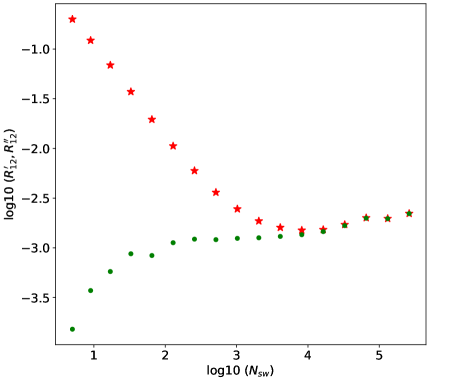
Figure 6: $R_{12}^{\prime}$ (red stars) and $R_{12}^{\prime\prime}$ (green dots) plotted against the smoothing window width $N_{sw}$, both in the log10 scale, for the SG filter.

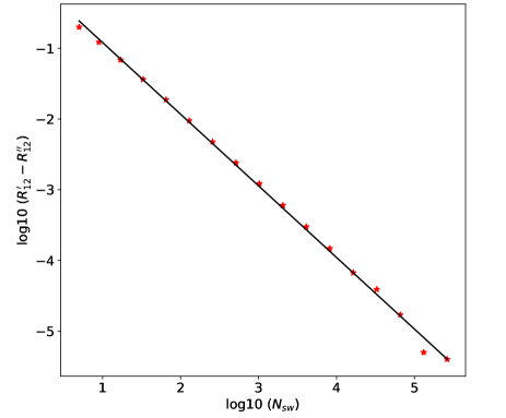
Figure 7: The difference $R_{12}^{\prime}-R_{12}^{\prime\prime}$ plotted against the $N_{sw}$, both in the log10 scale, for the SG filter.

Figure 7 shows the difference correlation $R_{12}^{\prime}-R_{12}^{\prime\prime}$ plotted against $N_{sw}$ for the SG filter. A least squares straight line fit yields the slope $-0.97\pm 0.01$ and intercept $0.03\pm 0.02$. Clearly this difference appears to decrease inversely with $N_{sw}$ so it tends to the value $0.0$ at large $N_{sw}$. So we can only use the smallest value of the difference (last data in Figure 7) as an upper limit for the correlation in Table 2. The errors in Table 2 are derived from the last three data in Figure 7, three being the minimum number of data required to estimate the standard deviation. Plots of $R_{12}^{\prime}-R_{12}^{\prime\prime}$ for the other two filters also show a similar trend with $N_{sw}$.

Similar plots have been made for the differences $R_{13}^{\prime}-R_{13}^{\prime\prime}$ and $R_{23}^{\prime}-R_{23}^{\prime\prime}$ for all three filters. These show a damped oscillation kind of trend around the value $0.0$, so they are also tending to the value $0.0$ at large $N_{sw}$. The smallest difference of these plots has been used as upper limit for the correlations in Table 2, as was done above, including for their errors.

In summary this section shows that there is almost no difference between $R^{\prime}$ and $R^{\prime\prime}$ as the smoothing filter estimates the smoothing function better by an increase of $N_{sw}$.

References

- Arons (1983) Arons, J. 1983, ApJ, 266, 215
- Arons (2009) Arons, J. 2009, Astrophysics and Space Science Proceedings "Neutron Stars and Pulsars", Eds. Werner Becker, pp 373, Springer.
- Arons (2011) Arons, J. 2011, Astrophysics and Space Science Proceedings "High-Energy Emission from Pulsars and their Systems", Proceedings of the First Session of the Sant Cugat Forum on Astrophysics, Eds. Nanda Rea & Diego F. Torres, pp 165, Springer.
- Arons & Scharlemann (1979) Arons, J. & Scharlemann, E.T. 1979, ApJ, 231, 854
- Bowley (1928) Bowley, A.L 1928, Journal of the American Statistical Association, Vol. 23, No. 161, pp 31; https://doi.org/10.2307/2277400
- Cerutti et al. (2016) Cerutti, B., . Philippov, A.A. and Spitkovsky, A. 2016, MNRAS, 457, 2401
- Cheng (2011) Cheng, K.S. 2011, Astrophysics and Space Science Proceedings "High-Energy Emission from Pulsars and their Systems", Proceedings of the First Session of the Sant Cugat Forum on Astrophysics, Eds. Nanda Rea & Diego F. Torres, pp 99, Springer.
- Cheng et al. (1986) Cheng, K.S., Ho, C. & Ruderman, M. 1986, ApJ, 300, 500
- Contopoulos et al. (1999) Contopoulos, I., Kazanas, D., Fendt, C. 1996, ApJ, 511, 351
- Contopoulos et al. (2019) Contopoulos, I., Petri, J., Stefanou, P. 2019, MNRAS, 491, 5589
- Goldreich & Julian (1969) Goldreich, P. & Julain, W.H. 1969, ApJ, 157, 869
- Harding & Grenier (2011) Harding, A.K. & Grenier, A. 2011, Astrophysics and Space Science Proceedings "High-Energy Emission from Pulsars and their Systems", Proceedings of the First Session of the Sant Cugat Forum on Astrophysics, Eds. Nanda Rea & Diego F. Torres, pp 79, Springer.
- Harding (2022) Harding, A.K. 2022, Astrophysics and Space Science Library 465 "Millisecond Pulsars", Eds. Sudip Bhattacharyya, Alessandro Papitto & Dipankar Bhattacharya, pp 57, Springer.
- Hermsen et al. (2013) Hermsen, W., Hessels, J.W.T., Kuiper, L. et al. 2013, Science 339, 436
- Hermsen et al. (2017) Hermsen, W., Kuiper, L., Hessels, J.W.T. et al. 2017, MNRAS466, 1688
- Hermsen et al. (2018) Hermsen, W., Kuiper, L., Basu, R. et al. 2018, MNRAS, 480, 3655
- Hirotani (2011) Hirotani, K. 2011, Astrophysics and Space Science Proceedings "High-Energy Emission from Pulsars and their Systems", Proceedings of the First Session of the Sant Cugat Forum on Astrophysics, Eds. Nanda Rea & Diego F. Torres, pp 117, Springer.
- Kirk et al (2009) Kirk, J.G., Lyubarsky, Y. & Petri, J. 2009, Astrophysics and Space Science Proceedings "Neutron Stars and Pulsars", Eds. Werner Becker, pp 421, Springer.
- Mereghetti et al. (2016) Mereghetti1, S., Kuiper, L., Tiengo, A. et al. 2016, ApJ, 831, 21
- Ostriker, & Gunn (1969) Ostriker, J.P. & Gunn, J.E. 1969, ApJ, 157, 1395
- Petri (2011) Petri, J. 2011, Astrophysics and Space Science Proceedings "High-Energy Emission from Pulsars and their Systems", Proceedings of the First Session of the Sant Cugat Forum on Astrophysics, Eds. Nanda Rea & Diego F. Torres, pp 181, Springer.
- Philippov et al. (2020) Philippov, A., Timokhin, A., Spitkovsky, A. 2020, Phys. Rev. Lett., 124, 245101
- Ruderman & Sutherland (1975) Ruderman, M.A. & Sutherland, P.G. 1975, ApJ, 196, 51
- Sobey et al. (2015) Sobey, C., Young, N.J., Hessels, J.W.T. 2015, MNRAS, 451, 2492
- Spitkovsky (2006) Spitkovsky, A. 2006, ApJ, 648, L51
- Spitkovsky (2011) Spitkovsky, A. 2011, Astrophysics and Space Science Proceedings "High-Energy Emission from Pulsars and their Systems", Proceedings of the First Session of the Sant Cugat Forum on Astrophysics, Eds. Nanda Rea & Diego F. Torres, pp 139, Springer.
- Sturrock (1971) Sturrock, P.A. 1971, ApJ, 164, 529
- Tennant et al. (2001) Tennant, A.F., Becker, W., Juda, M. et al. 2001, ApJ, 554, L173
- Tuo et al. (2019) Tuo, Y.L., Ge, M.Y., Song, L.M. et al. 2019, RAA, 19, 87
- Vivekanand (2020) Vivekanand, M. 2020, A&A, 633, A57
- Vivekanand (2021) Vivekanand, M. 2021, A&A, 649, A140
- Vivekanand (2022) Vivekanand, M. 2022, MNRAS, 514, 185