Discrepant Approaches to Modeling Stellar Tides, and the Blurring of Pseudosynchronization

Abstract

We examine the reasons for discrepancies between two alternative approaches to modeling small-amplitude tides in binary systems. The ‘direct solution’ (DS) approach solves the governing differential equations and boundary conditions directly, while the ‘modal decomposition’ (MD) approach relies on a normal-mode expansion. Applied to a model for the primary star in the heartbeat system KOI-54, the two approaches predict quite different behavior of the secular tidal torque. The MD approach exhibits the pseudosynchronization phenomenon, where the torque due to the equilibrium tide changes sign at a single, well-defined and theoretically predicted stellar rotation rate. The DS approach instead shows ‘blurred’ pseudosynchronization, where positive and negative torques intermingle over a range of rotation rates.

We trace a major source of these differences to an incorrect damping coefficient in the profile functions describing the frequency dependence of the MD expansion coefficients. With this error corrected some differences between the approaches remain; however, both are in agreement that pseudosynchronization is blurred in the KOI-54 system. Our findings generalize to any type of star for which the tidal damping depends explicitly or implicitly on the forcing frequency.

tablenum

1 Introduction

Sun et al. (2023, hereafter S23) introduce new functionality in the GYRE oscillation code (Townsend & Teitler, 2013; Townsend et al., 2018; Goldstein & Townsend, 2020) for modeling small-amplitude tides in binary systems. This functionality is implemented using a ‘direct solution’ (DS) approach, in which the differential equations and boundary conditions governing the radial dependence of tidal perturbations are solved directly as a two-point boundary value problem. To validate their implementation, S23 compare it against an alternative ‘modal decomposition’ (MD) approach popular in the literature (see, e.g., Press & Teukolsky, 1977; Kumar et al., 1995; Lai, 1997; Fuller & Lai, 2012; Burkart et al., 2012), where perturbations are expanded as a superposition of the star’s free-oscillation normal modes. An unexpected finding is that the secular tidal torques calculated using DS and MD differ significantly, casting doubt on whether the two approaches are truly equivalent.

In this paper we delve into the reasons for these differences. We focus on a model for the $2.32\text{\,}\mathrm{M}_{\odot}$ primary star of the highly eccentric ($e\approx 0.8$) heartbeat system KOI-54, constructed by S23 using the MESA stellar evolution code (Paxton et al., 2011, 2013, 2015, 2018, 2019; Jermyn et al., 2022). This model, about a third of the way through its main-sequence lifetime, has a convective core and a radiative envelope; as such, the principal tidal damping mechanism in the star is radiative dissipation. Most of our analysis is aimed at stars for which this is likewise the case, although we briefly discuss the relevance of our findings for other types of star.

The following section begins with a demonstration of the problem. In Section 3 we track down the reason for the differences between the MD and DS approaches, and in Section 4 we propose a fix to MD to resolve the issue. We reflect on the blurring of pseudosynchronization in Section 5, and then conclude in Section 6 with a summary and discussion of our findings.

2 Demonstrating the Problem

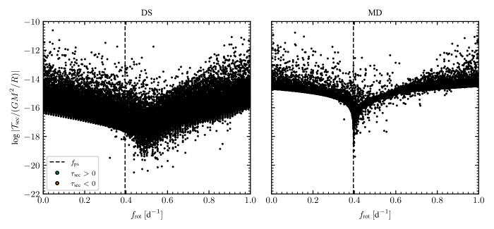
Figure 1: Secular torque $\mathcal{T}_{\rm sec}$ plotted against stellar rotation frequency $f_{\rm rot}$ for the KOI-54 primary model, as calculated using the DS approach (left) and the MD approach (right). In both panels, the vertical dashed line indicates the pseudosynchronous rotation rate $f_{\rm ps}$ given by equation (1).

Figure 1 demonstrates the differing predictions of DS and MD. Reprising Fig. 8 of S23, it plots the secular torque $\mathcal{T}_{\rm sec}$ due to the quadrupole tide as a function of stellar rotation frequency $f_{\rm rot}$, for the KOI-54 primary model. The two panels illustrate the outcome of using the DS approach (left; via gyre_tides) and the MD approach (right; via the formalism described in the following section). The torque is an extremely sensitive function of rotation frequency, varying by orders of magnitude as different free-oscillation modes are Doppler-shifted in and out of resonance; therefore, rather than attempting to plot continuous curves we sample the torque at 25,000 rotation frequencies randomly distributed in the interval $0\leq f_{\rm rot}/${\mathrm{d}}^{-1}$\leq 1$, and plot these data as discrete points in the figure.

The two panels agree in their general characteristics: torques are mostly positive at slow rotation rates, mostly negative at rapid rotation rates, and exhibit a lower envelope corresponding to the equilibrium tide (with departures from this envelope occurring near modal resonances.) However, the transition between the slow- and rapid-rotation limits occurs differently in each case. With MD, the equilibrium tidal torque passes through zero at $f_{\rm rot}=$0.395\text{\,}{\mathrm{d}}^{-1}$$, coinciding with the pseudosynchronous rate

$$f_{\rm ps}\equiv f_{\rm orb}\frac{1+(15/2)e^{2}+(45/8)e^{4}+(5/16)e^{6}}{[1+3e^{2}+(3/8)e^{4}](1-e)^{3/2}}$$ (1)

predicted by Hut (1981); here, $f_{\rm orb}$ is the orbital frequency. Within DS, however, the switch from positive to negative torque occurs over a range $1.1\lesssim f_{\rm rot}/f_{\rm ps}\lesssim 1.4$ of rotation frequencies, with equilibrium torques of opposite sign intermingling across this interval. We dub this ‘blurred’ pseudosynchronization. Away from the interval, the torque is one-to-two orders of magnitude smaller than in the MD case.

3 Diagnosing the Problem

3.1 Preliminaries

To explore the reasons for the discrepancies shown in Fig. 1, we first recapitulate some of the formalism from S23. The displacement perturbation vector $\boldsymbol{\xi}$ of a star, responding to strictly periodic tidal forcing by a companion, can be expressed as

$$\boldsymbol{\xi}(\mathbf{r};t)=\sum_{\ell,m,k}\left[\tilde{\xi}_{{\rm r};\ell,m,k}(r)\,\mathbf{e}_{r}\phantom{\left(\mathbf{e}_{\vartheta}\,\frac{\partial{}}{\partial{\vartheta}}\right)}\right.\\ \left.\mbox{}+\tilde{\xi}_{{\rm h};\ell,m,k}(r)\left(\mathbf{e}_{\vartheta}\,\frac{\partial{}}{\partial{\vartheta}}+\frac{\mathbf{e}_{\varphi}}{\sin\vartheta}\,\frac{\partial{}}{\partial{\varphi}}\right)\right]\\ \mbox{}\times Y^{m}_{\ell}(\vartheta,\varphi)\,\exp(-\mathrm{i}k\Omega_{\rm orb}t).$$ (2)

Here, $\mathbf{e}_{r}$, $\mathbf{e}_{\vartheta}$ and $\mathbf{e}_{\varphi}$ are the unit basis vectors in the radial ($r$), polar ($\vartheta$), and azimuthal ($\varphi$) directions, respectively; $Y^{m}_{\ell}$ is the spherical harmonic with harmonic degree $\ell$ and azimuthal order $m$; $\Omega_{\rm orb}\equiv 2\pi f_{\rm orb}$ is the orbital angular frequency; and the summations extend over $\ell\in[2,\infty]$, $m\in[-\ell,\ell]$ and Fourier-series index $k\in[-\infty,\infty]$. The Eulerian perturbation to the star’s self-gravitational potential is likewise given by

$$\Phi^{\prime}(\mathbf{r};t)=\sum_{\ell,m,k}\tilde{\Phi}_{\ell,m,k}^{\prime}(r)\,Y^{m}_{\ell}(\vartheta,\varphi)\,\exp(-\mathrm{i}k\Omega_{\rm orb}t),$$ (3)

and similar expressions exist for the perturbations to other scalar quantities.

The functions $\tilde{\xi}_{{\rm r};\ell,m,k}$, $\tilde{\xi}_{{\rm h};\ell,m,k}$ and $\tilde{\Phi}_{\ell,m,k}^{\prime}$ appearing in these expressions encapsulate the radial dependence of the response to the partial tidal potential $\Phi_{{\rm T};\ell,m,k}(\mathbf{r};t)$ (see equation 9 of S23). In the DS approach these functions are found by solving the two-point boundary value problem comprising the tidal equations and boundary conditions, as detailed in Appendix E of S23. In the MD approach, the functions are instead expanded as a superposition of the star’s adiabatic normal-mode eigenfunctions. Thus, for instance, $\tilde{\Phi}_{\ell,m,k}^{\prime}$ is expressed as

$$\tilde{\Phi}_{\ell,m,k}^{\prime}(r)=\sum_{n}A_{n,\ell,m,k}\,\hat{\Phi}_{n,\ell}^{\prime}(r)$$ (4)

where $\hat{\Phi}_{n,\ell}^{\prime}$ is the self-gravitational potential perturbation eigenfunction associated with the normal mode of harmonic degree $\ell$ and suitably-defined radial order $n$. Burkart et al. (2012) provide an expression for the expansion coefficients $A_{n,\ell,m,k}$ (see their equation 7); in the present notation this can be written

$$A_{n,\ell,m,k}=\frac{2\varepsilon_{\rm T}\,Q_{n,\ell}\,\bar{c}_{\ell,m,k}\,\Delta_{n,\ell,m,k}}{E_{n,\ell}}.$$ (5)

Here, the overlap integral $Q_{n,\ell}$ and normalized energy $E_{n,\ell}$ are defined in equations (9) and (10), respectively, of Burkart et al. (2012). The profile functions

$$\Delta_{n,\ell,m,k}\equiv\frac{\sigma_{m,k}^{2}}{(\hat{\sigma}_{n,\ell}^{2}-\sigma_{m,k}^{2})-2\mathrm{i}\hat{\gamma}_{n,\ell}\sigma_{m,k}}$$ (6)

encapsulate the frequency dependence of the expansion coefficients, with $\hat{\sigma}_{n,\ell}$ the mode eigenfrequencies, $\hat{\gamma}_{n,\ell}$ the damping coefficients, and

$$\sigma_{m,k}\equiv k\Omega_{\rm orb}-m\Omega_{\rm rot}$$ (7)

the angular frequency of tidal forcing in the frame co-rotating with the primary. Other symbols, here and subsequently, follow the definitions given in S23.

With the radial functions determined, the secular tidal torque plotted in Fig. 1 follows as

$$\mathcal{T}_{\rm sec}=4\Omega_{\rm orb}\sqrt{\frac{GM^{3}q^{4}}{1+q}}\,a^{1/2}\sum_{\ell,m,k\geq 0}\left(\frac{R}{a}\right)^{\ell+3}\,\left(\frac{r_{\rm s}}{R}\right)^{\ell+1}\\ \times\kappa_{\ell,m,k}\,\operatorname{Im}(\bar{F}_{\ell,m,k})\,\bar{G}^{(4)}_{\ell,m,k}$$ (8)

(from equation 25 of S23; the summation is now over non-negative $k$). The normalized response functions

$$\bar{F}_{\ell,m,k}\equiv-\frac{1}{2}\frac{R}{GM}\frac{\tilde{\Phi}_{\ell,m,k}^{\prime}(r_{\rm s})}{\bar{c}_{\ell,m,k}\varepsilon_{\rm T}},$$ (9)

with $r_{\rm s}$ the surface radius of the primary, are proportional to the tidal Love numbers $k_{\ell}$. These functions also appear in corresponding expressions for the secular rates-of-change of the orbital elements (see, e.g., equation 23 of S23), and the rate-of-work done by the tide (see Section 4); they are therefore an important output of any numerical tidal calculation.

3.2 Response Functions

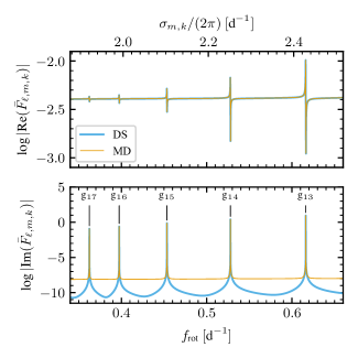
Figure 2: Normalized response function $\bar{F}_{\ell,m,k}$ plotted against stellar rotation frequency $f_{\rm rot}$, for the $\{\ell,m,k\}=\{2,-2,50\}$ partial tide of the KOI-54 primary model. The real (imaginary) part of the function is shown in the upper (lower) panel, and separate curves are plotted for the DS and MD approaches. Peaks are labeled by the resonant mode’s classification within the Eckart-Osacki-Scuflaire scheme. The upper axis scale shows the tidal forcing angular frequency $\sigma_{m,k}$ (equation 7).

We begin our diagnosis by comparing the normalized response functions predicted by the DS and MD approaches, for forcing by the $\{\ell,m,k\}=\{2,-2,50\}$ partial tidal potential in the KOI-54 primary model. Figure 2 plots the real and imaginary parts of $\bar{F}_{\ell,m,k}$ as a function of rotation frequency, following each approach. In both panels the distinct peaks corresponding to resonances with the star’s $\ell=2$ free-oscillation modes, and are labeled with the resonant mode’s classification within the Eckart-Osaki-Scuflaire scheme (see, e.g., Unno et al., 1989).

In the vicinity of the peaks both approaches appear to agree well. However, between the peaks the $\operatorname{Im}(\bar{F}_{\ell,m,k})$ data deviate significantly; the MD values are up to two orders of magnitude larger than the DS ones, and show a much weaker frequency dependence. These deviations are responsible for the discrepancies seen in Fig. 1.

3.3 Profile Functions

The deviations in Fig. 2 are frequency-dependent, and thus can only arise via the profile functions (6). To shed light on what might be amiss with these functions, we apply the MD formalism to the analogous but simpler problem of forced, damped transverse waves on a stretched string. Where appropriate, we draw direct parallels to the MD derivation by Kumar et al. (1995).

Let $\tau$ be the tension and $\mu$ the mass per unit length of the string; the equation of motion for small transverse displacements $u(x,t)$ is then

$$\frac{\partial^{2}\!{u}}{\partial{t}^{2}}=c^{2}\frac{\partial^{2}\!{u}}{\partial{x}^{2}}-2\gamma\frac{\partial{u}}{\partial{t}},$$ (10)

where $c\equiv\sqrt{\tau/\mu}$ is the wave speed, and the second term on the right-hand side models the damping as a velocity-dependent (Stokes) drag force governed by the coefficient $\gamma$. We assume the string is clamped at one end and subject to a transverse force $f(t)$ at the other, leading to the boundary conditions

$$u=0$$ (11)

at the clamped end ($x=0$) and

$$\tau\frac{\partial{u}}{\partial{x}}=f$$ (12)

at the forced end ($x=L$, with $L$ the string length).

To solve the stretched-string problem, we first reduce the non-homogeneous boundary condition (12) to a homogeneous one using the substitution

$$u(x,t)=v(x,t)+\frac{fx}{\tau}.$$ (13)

The wave equation (10) then becomes

$$\frac{\partial^{2}\!{v}}{\partial{t}^{2}}=c^{2}\frac{\partial^{2}\!{v}}{\partial{x}^{2}}-2\gamma\frac{\partial{v}}{\partial{t}}-\frac{x}{\tau}\left(\frac{\operatorname{d}^{2}\!\!{f}}{\operatorname{d}\!{t}^{2}}+2\gamma\frac{\operatorname{d}\!{f}}{\operatorname{d}\!{t}}\right),$$ (14)

and the boundary conditions are

$$v=0$$ (15)

at $x=0$ and

$$\frac{\partial{v}}{\partial{x}}=0$$ (16)

at $x=L$.

In the spirit of the MD approach, we assume solutions $v(x,t)$ can be expressed as a superposition of the spatial eigenfunctions that result from solving the homogeneous, undamped counterpart to the wave equation (14). Thus,

$$v(x,t)=\sum_{n=1}^{\infty}T_{n}(t)\sin(\omega_{n}x/c)$$ (17)

(cf. equation 1 of Kumar et al., 1995), where

$$\omega_{n}=\left(n-\tfrac{1}{2}\right)\frac{\pi c}{L}\qquad(n=1,2,\ldots)$$ (18)

are the eigenvalues. Substituting the trial solutions (17) into equation (14), and leveraging the orthogonality of the eigenfunctions, leads to an ordinary differential equation for each of the temporal coefficients $T_{n}(t)$:

$$\frac{\operatorname{d}^{2}\!\!{T_{n}}}{\operatorname{d}\!{t}^{2}}+2\gamma\frac{\operatorname{d}\!{T_{n}}}{\operatorname{d}\!{t}}+\omega_{n}^{2}T_{n}=F_{n}(t),$$ (19)

(cf. equation 2 of Kumar et al., 1995), where

$$F_{n}(t)=(-1)^{n}\frac{2c^{2}}{\omega_{n}^{2}\tau L}\left(\frac{\operatorname{d}^{2}\!\!{f}}{\operatorname{d}\!{t}^{2}}+2\gamma\frac{\operatorname{d}\!{f}}{\operatorname{d}\!{t}}\right).$$ (20)

Equation (19) has the familiar form of the second-order ordinary differential equation governing the motion of a forced, damped harmonic oscillator. For periodic external forcing

$$f(t)=f_{0}\exp(-\mathrm{i}\omega t),$$ (21)

steady-state solutions follow as

$$T_{n}(t)=(-1)^{n+1}\frac{2f_{0}c^{2}}{\omega_{n}^{2}\tau L}\frac{\omega^{2}+2\mathrm{i}\gamma\omega}{(\omega_{n}^{2}-\omega^{2})-2\mathrm{i}\gamma\omega}\\ \mbox{}\times\exp(-\mathrm{i}\omega t).$$ (22)

Combining this with equations (13) and (17), the steady-state solution to the original problem is

$$u(x,t)=\frac{2f_{0}c^{2}}{\omega^{2}\tau L}\sum_{n=1}^{\infty}(-1)^{n+1}\Delta_{n}\,\sin(\omega_{n}x/c)\\ \mbox{}\times\exp(-\mathrm{i}\omega t),$$ (23)

where the profile functions are

$$\Delta_{n}\equiv\frac{\omega^{2}}{(\omega_{n}^{2}-\omega^{2})-2\mathrm{i}\gamma\omega}.$$ (24)

(cf. equation 10 of Kumar et al., 1995). Comparing this result against the profile functions (6) arising in the MD approach for stellar tides, a noteworthy difference is that the damping coefficient in the latter is subscripted by the radial order $n$. We maintain that this is incorrect — as our analysis here of the stretched-string problem demonstrates, $\gamma$ should be independent of the summation index arising in the modal decomposition.

4 Fixing the Problem

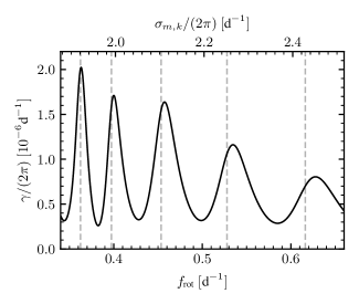
Figure 3: Damping coefficient $\gamma_{\ell,m,k}$ plotted against stellar rotation frequency $f_{\rm rot}$, for the $\{\ell,m,k\}=\{2,-2,50\}$ partial tide of the KOI-54 primary model. The dashed vertical lines correspond to the resonances shown in Fig. 2. The upper axis scale shows the tidal forcing angular frequency $\sigma_{m,k}$ (equation 7).

Based on the reasoning in the preceding section, we make the ansatz that the MD approach can be fixed by replacing the profile functions (6) with

$$\Delta_{n,\ell,m,k}=\frac{\sigma_{m,k}^{2}}{(\hat{\sigma}_{n,\ell}^{2}-\sigma_{m,k}^{2})-2\mathrm{i}\gamma_{\ell,m,k}\,\sigma_{m,k}},$$ (25)

where the damping coefficient $\gamma_{\ell,m,k}$ does not depend on $n$. To evaluate this coefficient we leverage energy conservation to write

$$\gamma_{\ell,m,k}=\frac{\mathcal{W}_{\ell,m,k}}{2\mathcal{E}_{\ell,m,k}}.$$ (26)

Here

$$\mathcal{E}_{\ell,m,k}=\sigma_{m,k}^{2}\int_{0}^{R}\left[\left|\tilde{\xi}_{{\rm r};\ell,m,k}\right|^{2}\right.\\ \mbox{}+\left.\ell(\ell+1)\left|\tilde{\xi}_{{\rm h};\ell,m,k}\right|^{2}\right]\rho r^{2}\,\operatorname{d}\!{r}$$ (27)

is the orbit-averaged total energy of the response to the partial tidal potential $\Phi_{{\rm T};\ell,m,k}$, and

$$\mathcal{W}_{\ell,m,k}=2\frac{GM^{2}}{a}q^{2}\left(\frac{R}{a}\right)^{\ell+3}\,\left(\frac{r_{\rm s}}{R}\right)^{\ell+1}\\ \times\operatorname{Im}(\bar{F}_{\ell,m,k})\,\sigma_{m,k}\,\bar{G}^{(5)}_{\ell,m,k}$$ (28)

is the orbit-averaged rate of work done on the star by this potential, with

$$\bar{G}^{(5)}_{\ell,m,k}\equiv\frac{2\ell+1}{4\pi}\left(\frac{R}{a}\right)^{-\ell+2}\left|\bar{c}_{\ell,m,k}\right|^{2}$$ (29)

(this definition means that $\bar{G}^{(4)}_{\ell,m,k}=m\bar{G}^{(5)}_{\ell,m,k}$). The factor of 2 in the denominator of equation (26) accounts for the fact that energy scales as the square of the response amplitude.

Because these expressions presume that solutions to the tidal equations are already known, their usefulness in stand-alone MD implementations may be limited. However, in the present case we can bootstrap their evaluation using solutions from DS approach. Fig. 3 plots the damping coefficient as a function of rotation angular frequency, evaluated from DS solutions for the same $\{\ell,m,k\}=\{2,-2,50\}$ partial tidal potential considered previously. The coefficient varies significantly with rotation frequency, with distinct peaks that correspond approximately to the resonances seen in Fig. 2.

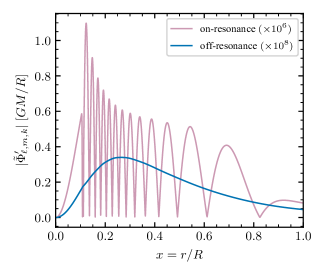
Figure 4: Eulerian self-gravitation potential perturbation $\tilde{\Phi}_{\ell,m,k}^{\prime}$ plotted against normalized radial coordinate $x$ for forcing on and off resonance with the ${\rm g}_{15}$ mode.

This behavior stems from the sensitivity of radiative dissipation to the wavelength of perturbations. Figure 4 plots the self-gravitational potential perturbation as a function of radial coordinate, obtained from the DS solutions at a pair of rotation frequencies: one tuned to resonance with the ${\rm g}_{15}$ mode, and the other equidistant between the ${\rm g}_{15}$ and ${\rm g}_{16}$ resonances. The on-resonance case shows the highly oscillatory, short-wavelength perturbations that are characteristic of dynamical tides, and is subject to strong radiative damping: $\gamma_{\ell,m,k}/(2\pi)=$1.5\text{\times}{10}^{-6}\text{\,}{\mathrm{d}}^{-1}$$. In contrast, the off-resonance case shows smooth, long-wavelength perturbations characteristic of equilibrium tides, and the damping is reduced to $\gamma_{\ell,m,k}/(2\pi)=$3.4\text{\times}{10}^{-7}\text{\,}{\mathrm{d}}^{-1}$$.

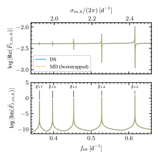
Figure 5: As in Fig. 2, except the MD approach uses the revised profile function (25) and damping coefficients bootstrapped using DS solutions (see Fig. 3).

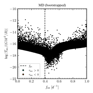
Figure 6: As in the right panel of Fig. 2, except using the revised profile function (25) and damping coefficients bootstrapped using DS solutions (see Fig. 3).

With $\gamma_{\ell,m,k}$ determined, Fig. 5 reprises Fig. 2 using the revised profile functions (25) in the MD approach. The agreement between DS and MD is greatly improved. As a further check, Fig. 6 reprises the right (MD) panel of Fig. 1, but again using the revised profile functions. There is now qualitative agreement between the two approaches, with MD showing the same blurred transition from positive to negative torque over a range centered on $f_{\rm rot}\approx$0.5\text{\,}{\mathrm{d}}^{-1}$$, as does DS. However, noticeable differences still remain; for instance, the MD torque values exhibit a lower envelope that’s around half an order of magnitude smaller than the DS ones, and they also show significantly less scatter.

These lingering differences may stem from terms in equation (5) other than $\Delta_{n,\ell,m,k}$; for instance, as remarked by S23, numerical estimates for the overlap integrals $Q_{n,\ell}$ can become inaccurate toward high radial orders. However, as an alternative explanation we draw attention to a more-fundamental limitation of the MD approach. In the stretched string problem we assume the damping coefficient $\gamma$ is spatially constant, and so the damping terms occur in the temporal equation (19). This assumption cannot be made in the stellar tides problem, because the radiative diffusivity varies by many orders of magnitude throughout a star. Therefore, when solutions of the form (2,3) are adopted, the damping terms instead appear in the spatial equations (see, e.g., Appendix E of S23). The adiabatic eigenfunctions are not solutions to these equations (a fact often overlooked in the literature), and the MD approach loses its formal coherence.

5 The Blurring of Pseudosynchronization

Regardless of their remaining differences, Fig. 1 (left) and Fig. 6 both agree that pseudosynchronization is blurred in the KOI-54 primary model. While we cannot offer a clear narrative for the characteristics of the blurring (e.g., why in this case it manifests over the range $1.1\lesssim f_{\rm rot}/f_{\rm ps}\lesssim 1.4$), it is straightforward to explain why equation (1) does not apply. Hut (1981) derived this equation within the weak friction approximation formalized by Alexander (1973), which presumes that the phase lag $\delta\phi$ between the tidal forcing and the response is proportional to $\sigma_{m,k}$. Within the MD approach with the revised profile function (25) the phase lag is given by

$$\delta\phi=\arg(\Delta_{n,\ell,m,k})=\tan^{-1}\left(\frac{2\gamma_{\ell,m,k}\sigma_{m,k}}{\hat{\sigma}_{n,\ell}^{2}-\sigma_{m,k}^{2}}\right).$$ (30)

Assuming $\gamma_{\ell,m,k}$ and $\sigma_{m,k}$ are both much smaller than $\hat{\sigma}_{n,\ell}$ (in accordance with the presumption of a weakly damped equilibrium tide), this approximates to

$$\delta\phi\approx\frac{2\gamma_{\ell,m,k}\,\sigma_{m,k}}{\hat{\sigma}_{n,\ell}^{2}}$$ (31)

When $\gamma_{\ell,m,k}$ itself depends on $\sigma_{m,k}$ (see Fig. 3, in particular the upper axis scale), it’s clear that strict proportionality between $\delta\phi$ and $\sigma_{m,k}$ cannot hold; therefore, the weak friction approximation does not apply, and the derivation of equation (1) breaks down.

If the original expression (6) for the profile functions is used instead of the revised one (25), the phase lag becomes

$$\delta\phi\approx\frac{2\hat{\gamma}_{n,\ell}\,\sigma_{m,k}}{\hat{\sigma}_{n,\ell}^{2}},$$ (32)

which is proportional to $\sigma_{m,k}$. This explains why Burkart et al. (2012) were able to reproduce equation (1) from their analysis (see their Appendix C2), and why their Fig. 4 and our Fig. 1 (right) show the equilibrium torque passing through zero at $f_{\rm rot}=f_{\rm ps}$.

6 Summary & Discussion

In the preceding sections we have demonstrated that a major source of disagreement between the DS and MD approaches is an incorrect damping coefficient in the MD profile functions (6). With the revised profile functions (25) the two approaches are brought into closer although still incomplete agreement. The practical issue of calculating damping coefficients $\gamma_{\ell,m,k}$ consistent with energy conservation, without needing to bootstrap from DS solutions, remains to be solved. One possible approach is to use a quasi-adiabatic treatment that estimates damping coefficients from an integral over the adiabatic tidal response — for instance, equation (14) of Burkart et al. (2012) modified to use the tidal response wavefunctions $\tilde{\xi}_{{\rm r};\ell,m,k}$, $\tilde{\xi}_{{\rm h};\ell,m,k}$ rather than individual modal eigenfunctions.

For stars like KOI-54 that have a convective core and a radiative envelope, dynamical tides arising through modal resonances are expected to be the dominant driver of orbital evolution (Zahn, 1975). This might imply that the highlighted issues with MD are of little consequence: as Fig. 2 shows, the MD and DS tidal response functions are in good agreement at the resonance peaks. However, the behavior of the tidal response in the approach to resonance peaks can be just as important as the peaks themselves in determining the evolutionary trajectory of a system. Consider for instance the phenomenon of resonance locking (Witte & Savonije, 1999), where orbital and stellar evolution conspire to maintain the frequency detuning $\delta\sigma=\hat{\sigma}_{n,\ell}-\sigma_{m,k}$ at a constant, small value over an extended period of time. The existence, location and stability of a resonance lock depends on the shape of the tidal response function in the wings of a peak (see, e.g., Fig. 1 of Burkart et al., 2014) — exactly where the deviations between MD and DS arise.

Although our analysis has focused mostly on the presentation of MD by Kumar et al. (1995) and Burkart et al. (2012), it extends to the broader variety of decomposition approaches — for instance, the phase-space mode expansion favored by Schenk et al. (2001) and Fuller (2017). Likewise, although we focus on stars with convective cores and radiative envelopes, our findings are relevant for systems with other internal architectures and other damping mechanisms. In any type of star where the damping coefficient explicitly or implicitly depends on the forcing frequency $\sigma_{m,k}$, switching to the revised profile functions (25) will alter the outcomes of MD-based calculations, and potentially uncover a similar blurring of pseudosynchronization. With this in mind, a careful re-evaluation of results in the existing stellar tides literature seems prudent.

While pseudosynchronization does not operate in KOI-54 in the manner originally envisaged by Hut (1981), Figs. 1 (left) and (6) nevertheless suggest that rotation frequencies of systems like KOI-54 will tend to accumulate in the range $1.1$–$1.4\,f_{\rm ps}$. This contrasts with the observational study of 24 heartbeat stars by Zimmerman et al. (2017), who find a majority of systems rotate at $\sim 0.66\,f_{\rm ps}$. Resolving this tension between theory and observation will be a productive direction for future investigations.

References

- Alexander (1973) Alexander, M. E. 1973, Ap&SS, 23, 459
- Astropy Collaboration et al. (2013) Astropy Collaboration, Robitaille, T. P., Tollerud, E. J., et al. 2013, A&A, 558, A33
- Astropy Collaboration et al. (2018) Astropy Collaboration, Price-Whelan, A. M., Sipőcz, B. M., et al. 2018, AJ, 156, 123
- Astropy Collaboration et al. (2022) Astropy Collaboration, Price-Whelan, A. M., Lim, P. L., et al. 2022, ApJ, 935, 167
- Burkart et al. (2014) Burkart, J., Quataert, E., & Arras, P. 2014, MNRAS, 443, 2957
- Burkart et al. (2012) Burkart, J., Quataert, E., Arras, P., & Weinberg, N. N. 2012, MNRAS, 421, 983
- Fuller (2017) Fuller, J. 2017, MNRAS, 472, 1538
- Fuller & Lai (2012) Fuller, J., & Lai, D. 2012, MNRAS, 420, 3126
- Goldstein & Townsend (2020) Goldstein, J., & Townsend, R. H. D. 2020, ApJ, 899, 116
- Hunter (2007) Hunter, J. D. 2007, Computing in Science & Engineering, 9, 90
- Hut (1981) Hut, P. 1981, A&A, 99, 126
- Jermyn et al. (2022) Jermyn, A. S., Bauer, E. B., Schwab, J., et al. 2022, arXiv e-prints, arXiv:2208.03651
- Kumar et al. (1995) Kumar, P., Ao, C. O., & Quataert, E. J. 1995, ApJ, 449, 294
- Lai (1997) Lai, D. 1997, ApJ, 490, 847
- Paxton et al. (2011) Paxton, B., Bildsten, L., Dotter, A., et al. 2011, ApJS, 192, 3
- Paxton et al. (2013) Paxton, B., Cantiello, M., Arras, P., et al. 2013, ApJS, 208, 4
- Paxton et al. (2015) Paxton, B., Marchant, P., Schwab, J., et al. 2015, ApJS, 220, 15
- Paxton et al. (2018) Paxton, B., Schwab, J., Bauer, E. B., et al. 2018, ApJS, 234, 34
- Paxton et al. (2019) Paxton, B., Smolec, R., Schwab, J., et al. 2019, ApJS, 243, 10
- Press & Teukolsky (1977) Press, W. H., & Teukolsky, S. A. 1977, ApJ, 213, 183
- Schenk et al. (2001) Schenk, A. K., Arras, P., Flanagan, É. É., Teukolsky, S. A., & Wasserman, I. 2001, Phys. Rev. D, 65, 024001
- Sun et al. (2023) Sun, M., Townsend, R. H. D., & Guo, Z. 2023, arXiv e-prints, arXiv:2301.06599
- Townsend et al. (2018) Townsend, R. H. D., Goldstein, J., & Zweibel, E. G. 2018, MNRAS, 475, 879
- Townsend & Teitler (2013) Townsend, R. H. D., & Teitler, S. A. 2013, MNRAS, 435, 3406
- Unno et al. (1989) Unno, W., Osaki, Y., Ando, H., Saio, H., & Shibahashi, H. 1989, Nonradial oscillations of stars, 2nd edn. (University of Tokyo Press)
- Witte & Savonije (1999) Witte, M. G., & Savonije, G. J. 1999, A&A, 350, 129
- Zahn (1975) Zahn, J.-P. 1975, A&A, 41, 329
- Zimmerman et al. (2017) Zimmerman, M. K., Thompson, S. E., Mullally, F., et al. 2017, ApJ, 846, 147