Arbitrarily weak head-on collision can induce annihilation
–The role of hidden instabilities–
Abstract
In this paper, we focus on annihilation dynamics for the head-on collision of traveling patterns. A representative and well-known example of annihilation is the one observed for 1-dimensional traveling pulses of the FitzHugh-Nagumo equations. In this paper, we present a new and completely different type of annihilation arising in a class of three-component reaction diffusion system. It is even counterintuitive in the sense that the two traveling spots or pulses come together very slowly but do not merge, keeping some separation, and then they start to repel each other for a certain time. Finally, up and down oscillatory instability emerges and grows enough for patterns to become extinct eventually (see Figs. 1-3). There is a kind of hidden instability embedded in the traveling patterns, which causes the above annihilation dynamics. The hidden instability here turns out to be a codimension 2 singularity consisting of drift and Hopf (DH) instabilities, and there is a parameter regime emanating from the codimension 2 point in which a new type of annihilation is observed. The above scenario can be proved analytically up to the onset of annihilation by reducing it to a finite-dimensional system. Transition from preservation to annihilation is also discussed in this framework.
1 Introduction
A variety of spatially localized structures emerge in many fields, such as gas discharge systems [3, 5, 62, 64], binary convection [35, 67], CO oxidation [4, 71], desertification [27, 19], oscillon [65], morphogenesis [70, 7, 6], and chemical reactions[34, 39, 18]. They may be stationary, time-periodic, or traveling patterns as coherent objects. It is noteworthy that, unlike elastic balls, those localized patterns can behave like a living cell, i.e., replication, coalescence, and annihilation according to environmental changes and external perturbations, such as collisions with other patterns or inhomogeneities in the media [2, 49, 50, 66, 51]. In other words, they are stable when isolated, but the hidden instabilities come out via interactions with the external world. To elucidate the mathematical mechanism behind these dynamics is a difficult task because they contain large deformations and strong nonlinear interactions. Nevertheless, by numerical exploration, we can decompose the process into the sequence of deformations forming a network of saddle solutions with decreasing Morse index, called the scattor-network developed by [49, 50], which gives us a good perspective of complex transient dynamics. For instance, suppose that two traveling spots collide at some point; then, whether they merge or not is controlled by a saddle type of stationary solution with a peanut shape called the scattor, in the sense that the solution orbit can be sorted out by the stable manifold of this scattor. See [49, 50, 51] for details and other examples of scattor-network.
However, it is possible to construct a rigorous method when we focus on a weak interaction among localized patterns, for instance, Ei et al. [10, 12] proposed a center manifold reduction method, in which the dynamics of pulse solutions can be described by low-dimensional ODEs as far as the solutions are well-separated and interact weakly (see also [8, 61, 63, 68]).
These two complementary approaches have enabled us to clarify the onset mechanism of the complex dynamics of localized patterns, such as self-replication, self-destruction, and oscillation of front and pulse solutions in one dimension [59, 60, 16, 36, 37, 17], pulse generators [58], and rotational motion of spots in two dimensions [56] and others (see references therein).
In this paper, we are particularly interested in annihilation dynamics, which is a typical phenomenon when two localized patterns collide strongly, as is well-known for the FitzHugh-Nagumo (FHN) pulses and BZ patterns [1, 2, 33], though the rigorous verification still remains open. An exceptional case is a class of scalar reaction diffusion equation in which one can control the large deformation of front waves, as shown in [20, 69]. The key ingredient here is an argument of comparison type; however, it cannot be applied to the systems discussed here.
The manner of annihilation of FHN pulses is intuitively clear because of the concentration of inhibitor contaminates around the colliding point, which leads to the collapse of the peak of the activator. We call this annihilation of fusion type (AF) for later use because the colliding patterns merge into one body before extinction. Annihilation of AF type can be understood by using the framework scattor-network mentioned above for traveling pulses of the Gray-Scott model and traveling spots of the three-component systems (1) and (2) (see [49, 50, 51] for details).
However, this is not a unique way that annihilation occurs at collision; in fact, a complete different type of annihilation of traveling spots has been found for the following three-component system of the FitzHugh-Nagumo type (1), as shown in Fig.1.
| (1) |
where as well as the diffusion coefficients are all positive constants. The system (1) was introduced by Purwins et al. [3, 5, 62, 64] as a qualitative model of gas-discharge phenomena, and many interesting dynamics of localized patterns have been demonstrated both in numerical and analytical approaches [49, 50, 53, 54, 55, 52, 58], especially in the excitable regime.
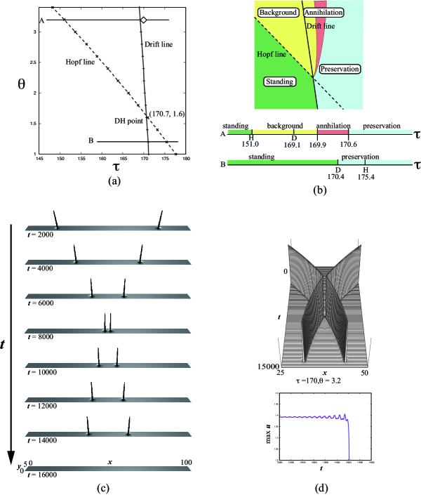
Apparently, it makes a sharp contrast with the fusion case. Firstly, the velocity of the spot is quite slow because the parameters are chosen close to the drift bifurcation point, as shown in Fig.1 (c)(d). Secondly, they almost keep the original shape even at the colliding point, though the distance between them at the nearest point is finite there. Thirdly, annihilation starts to occur in an oscillatory (up and down) manner after they rebound, and the extinction point is located far from the colliding point, as in Fig. 1 (d). This looks very counterintuitive because the two spots eventually annihilate even though they look like they are interacting each other very weakly. We call this weakly-interaction-induced-annihilation (WIIA), which makes a sharp contrast with AF type.
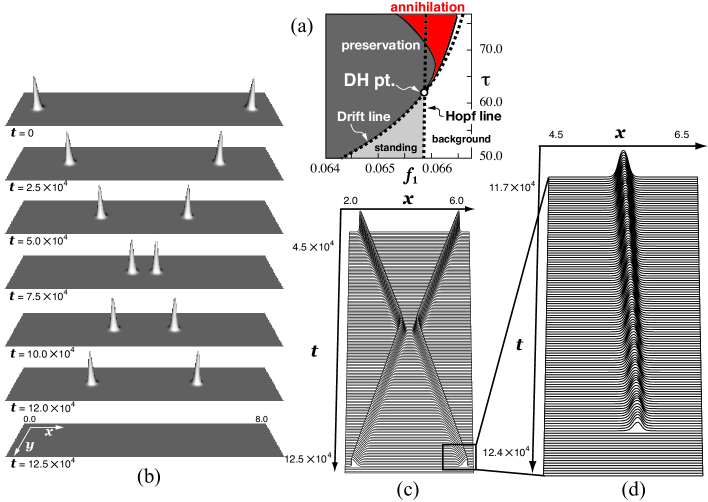
The above example is not an accidental numerical finding but rooted in a deeper structure, as will be clarified in this paper. In one word, it is a consequence of a hidden instability embedded in the localized pattern, which is triggered by the weak collision. Therefore, suppose that any other system shares the same mechanism; then, it shows similar dynamics. In fact, the following three-component system of activator-substrate-inhibitor type presents us another good example of WIIA, as shown in Fig.2.
| (2) |
where , and are all positive parameters related to inflow and removal rates of and and inhibition and decay rates for the inhibitor . The parameter controls the relaxation time for the inhibitor . The notation is the 2-dimensional Laplace operator. One of the origins of this model stems from an activator-substrate-inhibitor model developed by Hans Meinhardt [40] (see Chapter 5), who classified the shell patterns in the framework of reaction diffusion systems. Note that if the inhibitor is absent, then the system (2) is reduced to the Gray-Scott model.
The third component of the above two systems is crucial to sustain stable traveling patterns in higher-dimensional space and guarantees the coexistence of multiple stable localized traveling patterns in collision dynamics. In fact, the third component suppresses the elongation and shrinkage orthogonal to traveling direction and keeps them stable as localized patterns. Another advantage of the three-component system is to allow us to control the instabilities and their parametric dependency easily and detect the singularities of high codimension efficiently, as illustrated for pulse generators in [58] (i.e., double-homoclinicity of butterfly type).
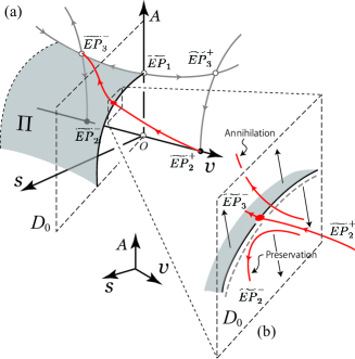
Our goal is to clarify the mathematical mechanism causing the WIIA from a dynamical system point of view, especially in the framework of hidden instabilities triggered by weak interaction. To accomplish the goal, we first have to understand how the traveling pattern can be pushed out of its basin by a weak external perturbation and what type of solutions form a basin boundary of it, which is one of the aforementioned scattors in collision dynamics. By closely looking at the behaviors of Figs.1 and 2, the up and down oscillation dominated the dynamics just before extinction in addition to the fact that the velocity is very slow; therefore, it is expected that a combination of drift and Hopf instabilities might play a crucial role behind the scenes. In fact, this is the case, and a set of unstable traveling breathers constitute the boundary of basin of traveling spots, and the size of its basin can be controlled by how close the parameters are to a codimension 2 point of drift-Hopf (DH) singularity. We will see in Section 3 that the basin size shrinks to zero as appropriate parameters tend to the DH point, which allows a very weak trigger to incur annihilation.
As already observed, the minimum distance point is not the place where annihilation occurs but is a turning point for the orbit to shift its dynamic regime from stable traveling spot to breathing motion.
The annihilation regime of WIIA type (indicated in Fig. 1 (a) and Fig. 2 (a)) can be obtained as one of the unfolding subsets of codimension 2 point of DH type; hence, such a codimension 2 point deserves to be called an organizing center producing a variety of dynamics including annihilation, though it is hidden when the pattern is isolated and only emerges through the interaction with other patterns or external perturbation.
Note that the codimension 2 point is not a generic situation; however, the unfolding subset, in which we observe WIIA robustly, is an open set emanating from the singularity, which will be explained in detail in the subsequent sections. In other words, WIIA is not a rare event, though it looks counterintuitive.
We will focus on the 1-dimensional case of (1) and justify the above scenario by reducing a PDE to finite-dimensional ODE dynamics near codimension 2 point of DH type. Such a reduction captures the essence of annihilation dynamics common to both 1-dimensional and 2-dimensional cases. A useful fact about the 1-dimensional case is that we have already many rigorous results of existence and stability properties [9, 21, 48]. Moreover, the information on eigenvalues and eigenfunctions around the codimension 2 singularity are available, which is crucial to obtain the reduced ODE system, as described later. It is of course possible to extend the method to higher-dimensional cases, but we leave this for the future work.
The remainder of the paper is structured as follows.
In Section 2, after introducing the 1-dimensional model system, we briefly explain how weak interaction induces annihilation by using the reduced ODEs. It turns out that the size of basin boundary of traveling pulse shrinks as parameters approach the DH singularity that causes annihilation of WIIA type. The existence of DH singularity is confirmed numerically in Section 2.3. In Section 3, we derive a finite-dimensional system around the DH singularity and show how the transition from preservation to annihilation occurs as parameters vary. We also compare the resulting dynamics with that of PDEs. Conclusions and outlooks are presented in Section 4.
2 1-dimensinal model system and main results
2.1 Three-component FHN system in 1-dimensional space
To gain deeper understanding of the qualitative description in Section 1, especially to understand the role of the unstable breather, we need to reduce the PDE dynamics to the finite-dimensional one and analyze the detailed mechanism behind it. We accomplish this task by using the three-component FHN system in 1-dimensional space (3), which completely inherits essential features of annihilation of WIIA type described in the previous section.
The reason for employing the model system (3) is firstly that it captures the essence of annihilation dynamics common to both 1-dimensional and 2-dimensional cases. Secondly, we also have many rigorous results of existence and stability properties [9, 21, 28, 24, 57, 48] for the 1-dimensional case. Finally, the information on eigenvalues and eigenfunctions around the codimension 2 singularity are computable, which is crucial to obtain the reduced ODE system, as described later.
The three-component system of the FHN type in 1-dimensional space reads as
| (3) |
An annihilation of WIIA type as depicted in Fig. 3 was originally presented in [14] for (3), in which the outline of the reduction to ODEs was also presented. In what follows, we shall show a more detailed and complete version of the reduction method, followed by precise analysis of the basin boundary between preservation and annihilation for the reduced system (11). This clarifies that the stable manifold of UTB forms a basin boundary of STP and how it behaves as parameters vary around the DH singularity depicted in Fig.4 (a).
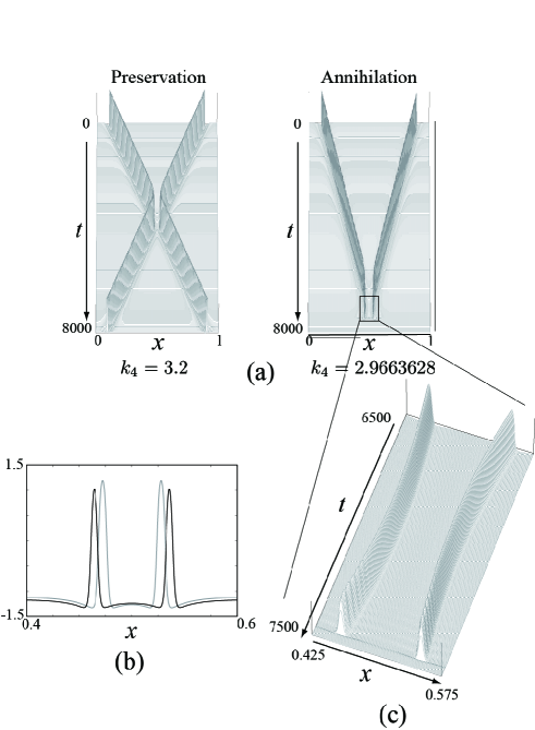
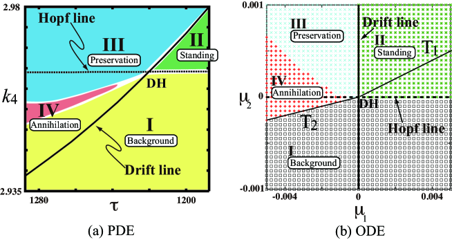
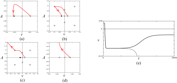
Figure 4 (a) shows the phase diagram of the outputs for the colliding pulse solutions, in which we draw the two lines of drift and Hopf bifurcations for the single pulse solution. The intersecting point is the DH singularity located at . The tongue of the annihilation regime almost touches the DH singularity, though it is not easy to detect it numerically. A typical transition from preservation to annihilation was observed as shown in Fig.3 (a), where is decreased from to with being fixed as . Note that this set of parameters is outside of the frame of Fig.4 (a). This is simply because the annihilation process is difficult to see visually if the parameters are too close to DH singularity. Figure 3 (b) shows two profiles of pulses for annihilation (solid black) and preservation (gray) cases when the distance between two pulses takes the minimum value for each case. An interesting point is that the distance for preservation is smaller than for annihilation. Figure 3(c) shows a magnification near the extinction point. The two traveling pulses collide very weakly and change their directions after collision, then up and down oscillation becomes visible. Finally, the pulses disappear suddenly. Meanwhile, the reduced ODEs show qualitatively the same phase diagram as in Fig.4 (b), which is the main theme of the next section.
At first sight, the manner of extinction in Fig. 3 looks counterintuitive, just like in Figs. 1 and 2. This is partly because it has been believed that only preservation can be observed when the pair of slowly moving pulses interact weakly through the tails; for instance, it was proved by weak perturbation method that this is the case for a special 22 reaction diffusion system of excitable type [12].
Historically, the classical 22 reaction diffusion system and its variants serve as one of the basic mathematical models for studying pulse dynamics. The existence of traveling pulses via drift bifurcation was established, for instance, by [31, 46]. Layer oscillations via Hopf bifurcation and standing breathers emanated from standing pulses have been studied both analytically and numerically [45, 32, 29]. The global bifurcation picture, including the four different pulse behaviors (standing pulses, traveling pulses, standing breathers, and traveling breathers) were studied in the singular limit system [30, 41, 43]. Stable traveling breathers were numerically detected in the narrow parameter region around the DH point [42].
These previous studies mainly focused on when and how the patterns of breathing type can be observed in various parameter settings, but this is only one side of the coin. Namely, they only focused on the half of the unfolding around DH singularity. In contrast to previous studies, we focus on the other half of the unfolding, i.e., super-critical drift and sub-critical Hopf bifurcations near DH point, and show that such a case can be realized for the system (3). This unfolding makes a change of the stability properties of bifurcated patterns, i.e., traveling breathers emanated from unstable traveling pulse as a secondary bifurcation are unstable and the basic traveling pulse recovers its stability instead. In the subsequent sections, we rigorously show that such unstable breathers exist and play a role of basin boundary for the annihilation dynamics of WIIA type in the framework of reduced ODEs near DH singularity.
2.2 Summary of the main results
It is instructive to present a brief summary of the main results for the reduced system. The details are presented in Section 3.
The reduced system for the “symmetric” head-on collision case describes the evolution of the distance between two pulses , the velocity (the other one is ), and the amplitude of Hopf instability . In fact, the growth of indicates the onset of annihilation. The principal part is given by the following system (see Section 3):
| (4) |
where and denote the deviations of parameter values from the codimension 2 point of DH singularity, and is defined by for . All the coefficients are positive, and is assumed to guarantee the super- (sub-)criticality of drift (Hopf) bifurcation. We also assume that (see (S6) in Section 3).
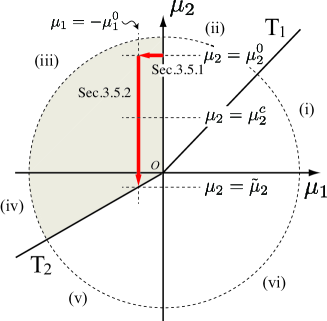
There are six different equilibria for (4) with , , which correspond to standing pulse (SP), standing breather (SB), traveling pulses (TPs), and traveling breathers (TBs) in the PDE sense, respectively. Note that means , namely, the above six equilibria represent the list of the “single” pulse that depends on the parameters. Here, indicates the traveling direction. Figure 5 presents the phase profiles projected to and the parametric dependency on . The equilibrium points in Fig.5 without indicate that those are critical points restricted to . The vertical (horizontal) line () is a drift (Hopf) bifurcation from . The two lines and denote the bifurcation curves of .
When we consider the symmetric collision, we focus on a special orbit starting from at . We are interested in the fate of this orbit after collision. When two pulses collide and rebound without annihilation, it is just a heteroclinic orbit connecting () to (). Meanwhile, when annihilation occurs, the orbit starting from collides with the other pulse, and oscillatory instability grows, i.e., the amplitude of becomes larger and eventually crashes to the background state. Therefore, it is natural to define the preservation and annihilation as follows.
Definition 1
When converges to as , the dynamics is called preservation.
Definition 2
When diverges as is increased, the dynamics is called annihilation.
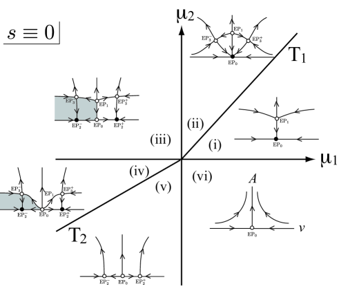
Note that the divergence of may occur at some finite . The transition from preservation to annihilation occurs as varies the region vertically from (iii) to (v) for a fixed negative in Fig.5.
Here, we briefly explain how the orbit can be pushed out of the basin of stable traveling pulse and annihilate via weak perturbation. The phase portrait of the single pulse of Fig.5 helps us to understand it at intuitive level. The basin of stable traveling pulse is a shaded region of Fig.5. Suppose the two pulses collide and interact weakly through the tails and still remain in the shaded region; then, loosely speaking, it is a preservation. As parameter is decreased and goes into region (iv), the basin starts to shrink and disappears in region (v). It is quite probable that the orbit can be kicked out of the basin in region (iv) and be extinct, which suggests that an arbitrary small external perturbation becomes a trigger for annihilation because the basin eventually disappears in region (v).
Our main theorem can be summarized as follows without technical terms; see Section 3 for more detailed assumptions and precise statements.
Theorem 1 (Preservation, annihilation, and shrinkage of basin)
The dynamics of symmetric head-on collisions is governed by (4). For any fixed sufficiently small , there exists a positive critical value , at which the orbit of (4) starting from reaches the scattor after collision. The outcome of an orbit starting from the above (below) is preservation (annihilation). The stable manifold of is the separator between preservation and annihilation. The transition from preservation to annihilation occurs due to the shrinkage of the basin of as is decreased.
2.3 Numerical verification of the existence of codimension 2 bifurcation point
In this section, we numerically investigate the existence of DH singularity for the system (3) and study the bifurcation structure around it.
-
•
Parameter setting: we employ and as bifurcation parameters in the sequel, and all other coefficients are fixed as , , , , , and , unless otherwise mentioned. For numerical integration, we adopt and , and the semi-implicit scheme is used for diffusion terms.
2.3.1 Global bifurcation diagram of single pulse
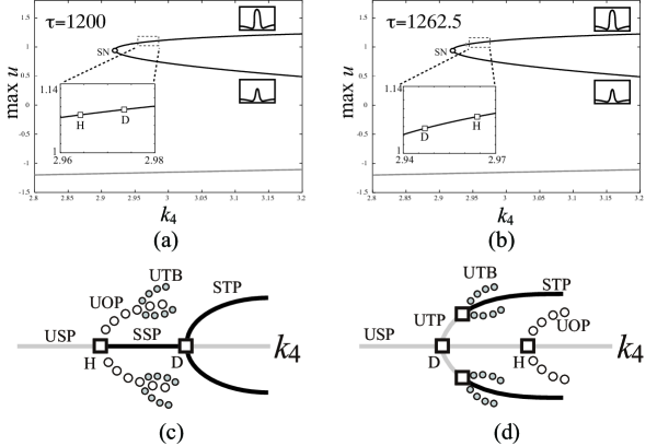
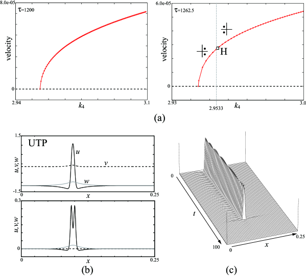
Figure 6 shows two global bifurcation diagrams of single standing pulse of (3) for (a) and (b) as varies. The secondary bifurcations of drift and Hopf instabilities are depicted in the magnified inlets, and their order is changed as is increased. Therefore, the codimension 2 singularity of DH type occurs in between. A schematic diagram of whole branches including secondary ones for each case is depicted in (c) and (d), from which we can extract key information on the transition from preservation to annihilation. We first take a close look at the solution behaviors around the secondary Hopf bifurcation for . Figure 7 (a) (left) shows a traveling pulse branch via drift instability at for . It is supercritical and inherits the stability of standing pulse. Note that the Hopf instability already occurred in the left side of it (outside of this frame), as shown in Fig.6(c). Meanwhile, the Hopf instability appears as a secondary bifurcation of the traveling pulse for (right), which is responsible for the recovery of stability of traveling pulse. Namely, the bifurcated oscillatory traveling pulse is of subcritical type and unstable, as shown in Fig.6(d). Prior to the Hopf point, the traveling pulse branch is unstable (UTP), and the real part of the associated unstable eigenfunction has a hollow in the middle, as shown in Fig.7 (b). This suggests that instability of UTP is a type of up and down Oscillation, as shown in (c), and the final destination is the background state.
2.3.2 Scattor and basin boundary regarding extinction
The unstable manifold of UTP is inherited to unstable traveling breather (UTB) due to the subcriticality of Hopf bifurcation; hence, if the orbit would be pushed outside of the basin of stable traveling pulse, then it would follow the behavior of unstable manifold of UTB, i.e., extinction occurs. In fact, the size of the basin of stable traveling pulse shrinks as approaches the Hopf point; therefore, a tiny external perturbation becomes a trigger of annihilation. We shall see the details of how this annihilation occurs in the reduced ODE system in Section 3. It turns out that UTB is a critical saddle solution emerging at the transition from preservation to annihilation, which is called a scattor in the study of collision dynamics [49, 50]. The unstable manifold of UTB plays a role of separator (basin boundary) between preservation and annihilation.
3 Reduction to pulse-interaction-ODEs for scattering dynamics
We describe the dynamics of widely-spaced localized patterns of reaction diffusion systems near DH point by reducing it to finite-dimensional ODEs in the general setting. The method to derive ODEs is quite similar to that developed by [10, 17, 12, 13, 16]. All the assumptions listed below can be checked numerically for (3). In this paper, we only perform formal derivation of ODEs and rigorous proof for the construction of an invariant manifold, and the derivation of the flow on it can be done in a parallel manner to those of references mentioned above.
3.1 Settings and assumptions
Let us consider the following general form of an -component reaction-diffusion system in 1-dimensional spaces
| (5) |
where , , is a smooth function, and and are diagonal matrices with positive elements. Here, we take and one of , e.g., , as bifurcation parameters and put , where and are small values. Later, we suppose that is the DH point (see (S1)). Then, (5) is rewritten as
| (6) |
where , , is an identity matrix, and is an matrix with and otherwise. We suppose . Let be the linearized operator of (6) with respect to and be the spectrum of .
The existence analysis of stationary pulse solution in this category was studied in [9, 48]. The codimension 2 singularity of DH type was rigorously detected in [21, 48]. Therefore, we assume the following properties:
-
(S1)
There exists a spatially symmetric stationary standing pulse solution and it has codimension 2 singularity of DH type at .
It has been proven that the tail of the pulse decays exponentially [9, 21, 48], and repulsive dynamics occurs through weak interactions (see (S4)). In fact, one of the components with the slowest decay rate dominates the weak interaction dynamics, and hence, we focus on the profile of the slowest component.
-
(S2)
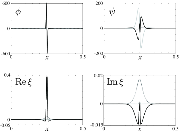
consists of and for some positive constant , and there exist three eigenfunctions , , and such that
where is the imaginary unit, is an even function, and and are odd functions (see Fig.8). The asymptotic behaviors of the slowest decay component of and are given as follows:
where is a positive constant and .
The profiles of , , and for (1) at codimension 2 bifurcation point DH are depicted in Fig.8.
-
(S3)
Let be the adjoint operator of . There exist , , and such that , , and . The asymptotic behaviors of the slowest decay component of and are given as follows:
where .
Under the assumptions (S1)–(S3), we have the following proposition.
Proposition 2
The functions , , and are uniquely determined by the normalization
3.2 Derivation of reduced ODE system
The derivation of the ODE system is based on the reduction method developed by Ei and his collaborators [10, 12, 13, 16, 17], which takes the following two steps: (i) construction of an invariant manifold under the conditions that the parameters are sufficiently close to the DH point and (ii) derivation of an ODE system describing the flows on it. The existence of an invariant manifold for the codimension 2 point of drift-saddle type has been proposed in [17], and the proof for our case, that is, the drift-Hopf type, can be done along the same lines as in the above references. Therefore, we omit the details of it and mainly focus on the derivation of the finite-dimensional ODE system on the invariant manifold.
We define as the set of all bounded operators from to . Because is identified with , we represent as , and as for simplicity. The third order derivatives are similarly defined.
We consider the dynamics of two weakly interacting pulses. Let , , be an adjoint operator of , and , where is the distance between two pulses. In a similar way to Propositions 3 and 4 of [10], we have the following propositions.
Proposition 3
There exist positive constants and such that for , the operator has four eigenvalues with (), and and have two eigenvalues each, and , and and , respectively, with (). Eigenvalues with multiplicities are repeated as many times as their multiplicities indicate. Other spectra of are on the left-hand side of for a positive constant .
Let and be the generalized eigenspaces corresponding to and , respectively.
Proposition 4
and are spanned by functions , and ,, respectively, for , and and are spanned by functions , and , , respectively, for .
hold, where , and here means .
Let and operators and be the projections from to and , respectively, where is the identity on . Let . Note that is characterized by
Now, we fix large enough such that Propositions3 and 4 hold. Fix with arbitrarily. Then, we can show that there exists a homeomorphic map from to for in a similar way to [10]. Let and be positions of pulses and . We take and with and sufficiently small.
Define and . Let be the solutions of the equations
where
and satisfy the following equations:
We define , , , and as follows:
where and , and we define as
Let and be the positions of pulses with , and the distance between the two pulses is given by . The quantities and are small-amplitude parameters. As explained later, and correspond to velocity and oscillatory amplitude of the left and right pulse, respectively. The ansatz is as follows:
| (7) |
for , where is the translation operator given by for .
We obtain a finite-dimensional ODE system, describing the dynamics of the position and velocity and the amplitude of oscillations near the DH point.
Proposition 5
Under assumptions (S1)–(S3), as long as and are sufficiently small and is sufficiently large, the dynamics of , , and are governed by the following equations:
| (8) | ||||
where represents the derivative with respect to ,
and
where . The constants , , and are given by
Theorem 6
Dynamics of two colliding pulses near DH point can be described as
| (9) | ||||
where , , , (), , . , , and . See Appendix B.2 for the definitions of and .
The proof of Theorem 6 is given in Appendix
B.2.
In our example, , , where
is the DH point shown in Fig.4(a).
We assume the following:
-
(S4)
The signs of and are positive.
This was confirmed numerically for (3). It is noted that means that two pulses interact repulsively. The principal part of (9) is given by
| (10) | ||||
The ODE system (9) looks close to the normal form of Hopf-Hopf type discussed in [38] (see Chap. 8.6). However, (9) contains an -variable so that it is not straightforward to prove that the principal part of (9) is conjugate to the full system. In the following, we first focus on the principal part (10). The validity of this approximation will be examined numerically in Sec. 3.6.
We are particularly interested in the ”symmetric head-on collision” case, namely, when the two pulses have a mirror symmetry, (10) becomes the following 3-dimensional system due to , which is the main object we analyze in the section.
Corollary 7 (Symmetric head-on collision)
The dynamics of the symmetric head-on collision is described by
| (11) | ||||
3.3 Bifurcation diagram of a single pulse
Prior to the detailed analysis of (11), it is instructive to investigate a bifurcation diagram of a single pulse solution. The dynamics of a single pulse is obtained by taking or for (11). Then, we have
| (12) | ||||
Note that the system (12) is the same as the amplitude equations of the truncated normal form of Hopf-Hopf bifurcation.
It is known that the phase diagram of equation (12) is qualitatively classified depending on (see [38]). We assume that satisfy the following:
-
(S5)
(13)
which was confirmed numerically for our system.
The phase portrait of (12) with (13) is shown in Fig.5 (see [38]). For any , (12) has a trivial equilibrium point
Equilibrium points with bifurcate at (Hopf line of PDE). We have for :
Equilibrium points with bifurcate at (drift line of PDE). We have for .
From and , the equilibrium points with bifurcate at
and
respectively. In view of the condition in (S5), we have in regions (ii), (iii), and (iv):
The solutions with and correspond to traveling breathers that play a key role as a separator. The bifurcation diagrams near the DH point shown in Fig.6(c) (resp.(d)) are qualitatively equivalent to the behaviors by varying (vi) (i) (ii) (iii) (resp. (vi) (v) (iv) (iii)) in Fig.5. Therefore, the ODE system (12) with (S5) describes the PDE dynamics of a single pulse solution quite well.
| Region | ||||
| (i) | stable | unstable | — | — |
| (ii) | stable | unstable | — | unstable |
| (iii) | unstable | unstable | unstable | |
| (iv) | unstable | — | stable | unstable |
| (v) | unstable | — | unstable | — |
| (vi) | unstable | — | — | — |
| the associated | ||||
| dynamics of a single | standing pulse | standing breather | traveling pulse | traveling breather |
| pulse solution | SP | SB | TP | TB |
The existence region of these equilibria in the parameter space and their stabilities (in the projected 2-dimensional space ) are summarized in Table 1. We note that coincides with for on , i.e., the basin size for shrinks as tends to . This is an important property to understand the switching mechanism from preservation to annihilation.
3.4 Definition of preservation and annihilation in the ODE system
The equilibria of Table 1 automatically become those of (11) by setting the third component as . Namely, the system (11) has a trivial equilibrium point
and nontrivial equilibrium points
Here, we added to the equilibria, indicating that they are the solutions of (11). Note that their stabilities are different from those in Table 1 as solutions of (11). When we consider the symmetric head-on collision, the initial value is specified as , meaning that the orbit starts from at . We are interested in the fate of this orbit after collision.
We define , , and by
The equilibrium point is given by , and is given by . We define the following functions:
| (14) | ||||
where and satisfy and when , respectively.
Let us define the terminologies “preservation” and “annihilation” for the ODE system. The annihilation contains a large deformation, so we can prove something about its onset here, namely, the amplitude of oscillation grows and the orbit does not come back to any equilibrium point of (11). Therefore, it is reasonable to use the amplitude of oscillation as a criterion for annihilation because annihilation is caused by subcritical Hopf bifurcation.
Definition 3 (Preservation and annihilation)
When the solution converges to as for a given set of parameters, we call it “preservation”. On the contrary, when the variable of the solution diverges, we call it “annihilation”.
3.5 Symmetric head-on collision
Now, we are ready to study (11), especially the parametric dependency of the orbit starting from at , which is associated with a stable traveling pulse in regions (iii) and (iv) in the parameter space of Fig.9 (see also Fig. 5). We shall show that preservation is observed in region (iii), and the transition from preservation to annihilation occurs at some point in region (iv) as is decreased. The equilibrium point has a positive eigenvalue for . In the following, as a convention, we take an initial condition on the corresponding unstable manifold of , unless stated explicitly. In Sec.3.5.1, we show the transition from standing to preservation as is decreased for a fixed . In Sec.3.5.2, we fix , and is decreased from to the line . We show the existence of the critical point at which the solution orbit lies on the stable manifold of separating two regions of preservation and annihilation.
We define the following regions:
We see from (11) that increases and decreases when the solution is in and , respectively. The two traveling pulses start to repel each other when the solution orbit moves from and .
Before going into the detail, we briefly outline the proof here. First, let us define the time as the first hitting time of the solution at , where we take when the solution does not hit it. We also define the time as the first hitting time when the variable reaches , where we take when the solution does not hit it. The preservation dynamics is roughly divided by the following three steps. In the first step (), the solution trajectory takes off from , and increases and reaches the maximum value when the solution touches (see the proof of Lemma 9). In the second step (), decreases and approaches the plane. In the final step (), the solution converges to . To prove the existence of the preservation parameter regime and the heteroclinic orbit from to in the validity regime of weak interaction, we need to estimate , , and for each step.
The following lemma will be used to estimate the maximum of , i.e., the minimum distance of the colliding pulses.
Lemma 8
Let be a positive constant. The function
is monotonically decreasing. There exists a unique such that with if satisfies .
Proof 1
Because , it holds that
where we used the fact that the function () is monotonically increasing for . From the condition , the Taylor expansion of the right-hand side of reads as
Thus, .
The following lemma gives an upper bound of when the solution is in and the solution trajectory of (11) enters in a finite time.
Lemma 9
Let assumptions (S1)–(S5) hold. Assume that for some and . Then, it holds that
-
1.
and for ,
-
2.
is finite, and
-
3.
attains the maximum value at .
Proof 2
When , from the conditions and , it holds that for (Fig.10(a)). That is, for .
We take and as given in Lemma 8. Assume that there exists such that . From the definition of , holds for . We will prove that before reaches . From (11), we have
| (15) |
Integrating both sides of (15) during , we have
| (16) |
Therefore, for , where we used properties that the right-hand side of (16) is monotonically increasing and attains at . Meanwhile, for , it follows that
| (17) | ||||
where we used , , and . Integrating both sides of (20) during ,
Here, we have used Lemma 8 and .This implies that , i.e., is finite. The variable has the maximum value for because the sign of determines the sign of . Thus, holds, that is, for . Because decreases in , for , that is, for .
3.5.1 Existence of preservation region –Decreasing from the drift line () with being fixed–
Suppose that is fixed and decreasing from the drift line () (Fig.9). The dynamics of (11) around is described as follows:
| (18) | ||||
These equations are obtained by applying the center manifold theory around the drift point . The variable is described by the following algebraic equation on the center manifold:
| (19) |
Lemma 10
Let assumptions (S1)–(S5) hold and be fixed. If is taken sufficiently close to , then for all .
Proof 3
Theorem 11 (preservation)
Let assumptions (S1)–(S5) hold and be fixed. If is taken sufficiently close to , the solution converges to .
Proof 4
From the center manifold theory in Appendix B, and can be taken as arbitrarily small for by taking sufficiently smaller than . Thus, from Lemma 10 and (19), holds for because and for sufficiently small . Thus, from Lemma 9, we find that the solution crosses in finite time.
Because ,
This means that the solution belongs to for , and there exists and such that for . That is, as because for , and for (see the phase portrait for in Fig.5 (iii)).
This theorem indicates that the drift line is the boundary between the standing and preservation regions. We remark that because and can be arbitrarily small as , the maximum value of tends to as . This implies that no annihilation occurs for sufficiently small when is fixed.
3.5.2 Transition from preservation to annihilation –Decreasing from with being fixed–
Next, we will show that there exists a critical value at which the solution trajectory lies on the stable manifold of (denoted by in Fig.10). As shown in the phase portrait in Fig.5, it is plausible that diverges when is taken close to on in Fig.9. Hence, it follows almost immediately from Theorem 11 and the continuity of the solution with respect to the parameters that there exists a critical where the solution trajectory crosses the stable manifold of between and . However, because the reduced ODE is valid in the weak interaction regime, we need to show that , and for when . For this purpose, we introduce an invariant set satisfying the property that the orbit diverges once it enters .
Before defining , we examine the number of common points of the curve (recall the definition (14)) and the line in the region and , where is a constant in the interval . Because , the equation should have a solution . We denote the other solution by (see the magnified inset in Fig.10 (a)), where
We also define
| (21) |
The equation has a multiple root at , where
By direct computation, we have
Thus, decreases as is decreased. Therefore, in the region and , the curve and line have one common point when and two common points when [Fig.10 (a)].
Now, we define by
| (22) | ||||
where for and for [Fig.10 (a)]. We will see in the next lemma that is designed such that becomes an invariant set.
Because is convex and the slope of at is smaller than that at , the plane does not have an intersection with the plane for and the plane for [Fig.10 (a)].
-
(S6)
.
Under assumption (S6), we shall show in the next lemma that becomes an invariant set and that if the orbit enters into , then has to diverge to .
The following lemma gives a sufficient condition for the divergence of .
Lemma 12
Let assumptions (S1)–(S6) hold. If the solution enters in finite time, then diverges.
Proof 5
We investigate the flows at the boundary of .
Case 1:
The normal vector at a point on is and
and on . Thus, we obtain
where we used (S6). This implies that the solution trajectory directs to the interior of on .
Case 2:
For a point on , because , we have
Case 3:
For on , because on , we have
Now, it is clear that is invariant.
Next, we show that diverges if the solution once enters . Suppose that the solution trajectory touches the boundary of at . Because and , there exist and such that for . Because and for , we have
Thus, we find as is increased.
Lemma 13
If is in the preservation region, and for all .
Proof 6
Let us define the following set:
Firstly, we show that in . Assume that the solution trajectory touches the plane in . Because and on in , the solution does not cross the plane in . Thus, the solution diverges in or crosses and enters . For both cases, diverges, which contradicts the condition that is taken in the preservation regime. Thus, for , where is the time when touches the plane .
Secondly, we show that for . Because is taken in the preservation regime, for ( is the time when attains ) from Lemma 12. It follows from Lemma 9 that for , especially . We estimate the minimum value of for . Let us define by the time when reaches again, where if does not. For , it holds that
where we used because and for . Therefore, it follows that
| (23) |
Because is taken in the preservation regime, from Lemma 12, the solution does not enter at . That is,
should hold as long as holds for from the definition of (see Fig.10). Because (Lemma 9) and , by using (23), we have the following estimation for :
That is, it follows that
Thus, for .
If attains again at , we can show that for by using the same argument. Therefore, for , and we find for .
From these lemmas, we find that the variables , , and are sufficiently small as long as belongs to the preservation regime.
Lemma 14
Let assumptions (S1)–(S6) hold. For , the unstable manifold emanating from consists of two parts: one-half of it converges to and the other half enters . That is, is a separator between preservation and annihilation.
Proof 7
The Jacobian matrix corresponding to is given by
The matrix has eigenvalues
where the signs of the eigenvalues are for .
We show that unstable manifolds emanating from enter the region for , where is a region surrounded by the plane and in the plane (Fig.11). That is, one of the unstable manifolds of belongs to , and the other converges to .
For , or , the eigenvector corresponding to is given by , where
Because , it holds that
Theorem 15 (Traveling breather as a separator between preservation and annihilation)
Let assumptions (S1)–(S6) hold. If and is decreased from , then the solution of (11) converges to at some , namely, the orbit lies on the stable manifold of the separator between preservation and annihilation. For any orbit with initial data above (below) this manifold, its component diverges (it converges to ).
Proof 8
Firstly, we show that annihilation occurs when . Let us define by
We show that the unstable manifold, emanating from , corresponding to the positive eigenvalue , enters . The Jacobian matrix of is
The eigenvector corresponding to the unstable eigenvalue is
Because , , and , it follows that
By noting that is the slope of the line , we find that the solution trajectory emanating from enters .
The solution trajectory does not cross the plane in because
where we used and on the plane in .
Now, we take . We will show that
where was defined in (21) and the left side is the -intercept of the line (Fig.12). Namely, if is satisfied, the solution trajectory emanating from enters , which means that annihilation occurs for from Lemma 12. Let us proceed to prove the above inequality. At ,
When , it holds from (S6) that
When , it holds from (S6) that
where we note that
from (S5) and (S6).
Finally, we show that there exists such that the solution trajectory converges to the separator between preservation and annihilation at . The solution trajectory converges to at by definition (preservation), while at the same time, it follows from the above arguments that the solution trajectory enters when . Then, we conclude from the continuous dependency of the trajectory on the parameters that there exists at least one such that the solution lies on the stable manifold of at some (Fig.13). In other words, the stable manifold of is a separator between preservation and annihilation.
Remark 1
The uniqueness of the critical parameter is not known in Theorem 15; however, if it holds and the transversal property is satisfied at , then preservation and annihilation regimes are completely separated by .
3.6 Comparison with PDE dynamics
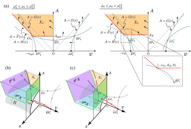
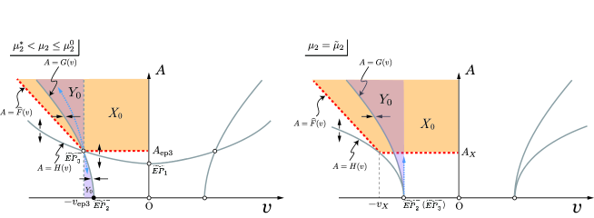
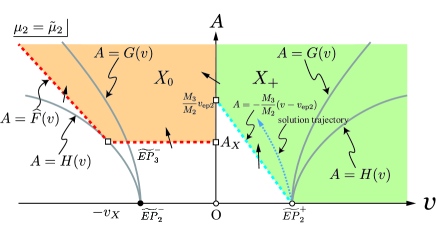
Let us confirm numerically that the reduced system (11) gives us qualitatively the same phase diagram as that of the PDE model (see Fig.4(a)). In numerical simulations, the initial data is taken near if it exists and is taken near if it does not (see Appendix A for details). Recall that the criterion for the occurrence of “annihilation” is that the component diverges, and “preservation” means that the solution converges to . The background state shows the non-existence of both standing and traveling pulses. The ODE phase diagram Fig.4(b) is obtained based on this classification. Fig.14 shows typical orbital behaviors depending on the parameters. It is clear from previous discussions that the Hopf and drift lines separate background, standing, and preservation regions counterclockwise like I II III, similar to the PDE diagram. The transition from preservation to annihilation occurs as is decreased and the lower boundary of the annihilation regime is . The most subtle issue is to examine whether the tongue of the annihilation regime touches the DH point or not, which is unclear due to the limitation of numerical discretization.
The following analytical result helps us to resolve the issue, which is obtained directly from Theorem 15.
Corollary 16
Let assumptions (S1)–(S6) hold. Then, we have as .
Proof 9
Because the preservation dynamics is observed for () arbitrarily close to the origin, the critical can be taken arbitrarily close to from Theorem 15.
Theorem 15 indicates that the solution trajectory approaches UTB at after weakly symmetric collision. In addition, from Corollary 16, the tip of the annihilation region touches the DH point, and WIIA occurs for arbitrarily slow and weak collisions. This suggests that annihilation occurs for any arbitrary slowly colliding pulses of the PDE system (3), which is not an easy task to realize by numerical simulations. However, if we choose a set of parameter values carefully in the annihilation regime (but close to the border between annihilation and preservation), we observe the behavior depicted in Fig.3. In fact, it does not look like a collision because they are well-separated even at the nearest point. They rebound after that and start to oscillate up and down before collapsing to the background state. The last stage indicates that the PDE solution actually behaves like the separator UTB.
At first sight, this looks contradictory to the results in [12], in which they showed that preservation occurs when two pulses collide weakly enough. However, in our case, the criterion of the fate of the dynamics is not strength of interaction but the size of basin of attraction of preservation, which is essentially a different viewpoint from that in [12]. In fact, as shown in Fig.3(b), the minimum distance of two pulses in the annihilation regime is larger than that for preservation, which suggests that the strength of interaction is not a main factor causing annihilation.
Overall, both the PDE and reduced ODEs present qualitatively the same phase diagrams, as depicted in Fig.4. The reduced ODEs clearly show the location of transitions and how they happen there; in particular, the transition from preservation to annihilation is highlighted in the previous section.
4 Conclusion and outlook
-
•
Codimension 3 singularity:
We considered the hidden instability of DH type in this paper. It is a combination of drift and Hopf instabilities. The meaning of ”hidden” is that it is not visible when the pattern is isolated. It comes out when the pattern starts to interact with other traveling patterns or defects. A nontrivial characteristic is that even if they interact very weakly, they experience a large deformation and annihilate each other provided that all the parameters are chosen close to the DH point. In a sense, the pattern is very fragile when it includes such instabilities inside. There is one thing we have to pay slightly more attention to understand the dynamics of annihilation: the existence of a saddle-node bifurcation of the standing pulse branch, as shown in Fig.6(a)(b). In fact, annihilation heavily depends on the saddle-node point that determines the destinations of the unstable manifolds of UTP and UTB (i.e., homogeneous background state). In this paper, we assumed that the destinations of UTP and UTB are the background state and did not consider the effect explicitly coming from the saddle-node bifurcation. It would be reasonable to consider the annihilation in the framework of codimension 3 singularity, i.e., DH point + saddle–node bifurcation; however, we leave this as a future work. -
•
Global structure of PDE branches:
It is an interesting future task to explore the global behaviors of PDE solution branches as schematically depicted in Fig.6(c)(d). In particular, unstable traveling breathers UTB play a key role in understanding the transition from preservation to annihilation; therefore, more precise bifurcation structure of secondary branches may help us to explore the behavior of the basin structure of traveling pulses. -
•
2-dimensional spot annihilation:
We showed the annihilation of 2-dimensional spots in Section 1 for the two representative three-component reaction diffusion systems. It is possible to derive a similar reduced finite-dimensional system associated with the 2-dimensional case, as we did in Section 3. We believe that the same mechanism of annihilation as the 1-dimensional case works also for the 2-dimensional case; however, more careful analysis is needed due to the increase of unknowns, this remains as a future work. -
•
Oblique collision and coherent motion of many traveling spots:
The search for a coherent motion of many traveling spots is an interesting open question. It is numerically observed that if each traveling spot is robust (i.e., not close to hidden instabilities), then repulsive interaction drives them to the marching mode (i.e., travel in the same direction with same velocity) in a bounded domain with periodic boundary condition. However, for the spots close to DH singularity, they may annihilate upon collision when they are close to a head-on collision. It is not known how the angle between two traveling spots affect the outcome after collision, what is the asymptotic behavior as time goes on, and how the final state depends on the density of spots. -
•
Heterogeneous media Defects or heterogeneities in the media is another type of external perturbation to propagating spots and pulses, which may trigger pinning to the defects, as was shown in [23, 44, 25, 26]. Suppose a propagating pulse or spot has a hidden instability of DH type; then, it is natural to observe a similar annihilation after collision against a defect. It is confirmed numerically that a 1-dimensional traveling pulse experiences a similar annihilation to that depicted in Fig.3. For higher-dimensional cases, we conjecture that the same type of annihilation occurs, but the details are left as a future work.
Appendix A Phase diagram for the reduced ODE
In the numerical simulations for (11), the initial data is taken near if exists and is taken near if does not:
Figure 4(b) shows the phase diagram. Here, in convenience, we suppose the criterion for the occurrence of “annihilation” is that reaches . When the solution converges to , , the dynamics is called “standing” and “preservation”, respectively. The region “ background” corresponds to the parameter region where no stable solution exists.
Appendix B Proof of Proposition 5 and Theorem 6
B.1 Proof of Proposition 5
By expanding the right hand side of (27), we have
B.2 Proof of Theorem 6
In order to vanish quadratic terms with respect to and , we perform a smooth invertible transformation:
| (29) | ||||
where
Differetiating both side of (29) and substituting into (8), we have
where
In order to derive an amplitude equation (9), we change as .
Appendix C The derivation of (19)
We consider the following equation around :
| (30) | ||||
The linearized matrix of (30) is
and the eigenvalues are . The eigenvector corresponding to is given by the following equation:
Thus, we have . Another eigenvalue for is given by the following equation:
Thus, we have . The eigenvector corresponding to is given by
Thus we have . Therefore the transformation matrix is given by
Therefore it holds that
Here we take
That is, , , . Substituting these into (11), we have
In order to apply the center manifold theory, we take as a function of and consider the follwoing equations
| (31) | ||||
Since , the variable on the center manifold can be expressed by the quadratic equation:
| (32) |
where . By differentiate both sides of (32) using (31), we have
| (33) |
On the other hand, putting (32) in the equation of (31), whe have
| (34) |
Comparing the second order terms between (33) and (34), we have , , . Therefore,
Thus, we obtain
acknowledgment
This work was supported by KAKENHI 20K20341, 22H05675, 20K03730, and 23K03209.
References
- [1] M. Argentina, P. Coullet and L. Mahadevan, Colliding Waves in a Model Excitable Medium: Preservation, Annihilation, and Bifurcation, Phys. Rev. Lett. 79 (1997), pp. 2803–2806.
- [2] M. Argentina, P. Coullet and V. Krinsky, Head-on Collisions of Waves in an Excitable FitzHugh-Nagumo System: a Transition from Wave Annihilation to Classical Wave Behavior, J. theor. Biol. 205 (2000), pp. 47–52.
- [3] Yu. A. Astrov, H.-G. Purwins, Plasma spots in a gas discharge system: Birth, scattering and formation of molecules, Phys. Lett. A 283 (5-6), pp. 176–198.
- [4] M. Bär, M. Eiswirth, H. -H. Rotermund, and G. Ertl, Solitary-wave phenomena in an excitable surface reaction, Phys. Rev. Lett. 69 (1992), pp. 945–948.
- [5] M. Bode, A. W. Liehr, C. P. Schenk and H. -G. Purwins, Interaction of dissipative solitons: particle-like behaviour of localized structures in a three-component reaction-diffusion system, Physica D 161 (2002), pp. 45–66.
- [6] J. Cotterell, A. Robert-Moreno, and J. Sharpe, A local, self-organizing reaction-diffusion model can explain somite patterning in embryos, Cell Systems, 1(4) (,2015), pp. 257–269.
- [7] V. Brena-Medina and A. Champneys, Subcritical turing bifurcation and the morphogenesis of localized patterns Phys. Rev. E, 90 (2014), pp. 032923.
- [8] A. Doelman and T. J. Kaper, Semistrong pulse interactions in a class of coupled reaction-diffusion equations, SIAM J. Appl. Dyna. Sys., 2(1) (2003), pp. 53–96.
- [9] A. Doelman, P. van Heijster , T. J. Kaper, Pulse dynamics in a three-component system: existence analysis, J. Dyn. Diff. Eq., 21 (1) (2009), pp. 73–115.
- [10] S. -I. Ei, The motion of weakly interacting pulses in reaction diffusion systems, J. Dyn. Diff. Eqs., 14(1) (2002), pp. 85–137.
- [11] S. -I. Ei, H. Ikeda and T. Kawana, Dynamics of front solutions in a specific reaction-diffusion system in one dimension, Japan J. Indust. Appl. Math. 25(1) (2008), pp. 117–147.
- [12] S. -I. Ei, M. Mimura, and M. Nagayama, Pulse-pulse interaction in reaction-diffusion systems, Physica D, 165 (2002), pp. 176–198.
- [13] S.-I. Ei, M. Mimura, and M. Nagayama, Interacting spots in reaction diffusion systems, Discrete Contin. Dyn. Syst. 14(1) (2006), pp. 31–62, doi: 10.3934/dcds.2006.14.31
- [14] K. -I. Ueda, T. Teramoto, and Y. Nishiura Scattering of particle-like patterns in reaction-diffusion systems, Gakuto International Series, Mathematical Sciences and Applications, 22 (2005), pp. 205–215.
- [15] S. -I. Ei, K. Nishi, Y. Nishiura, and T. Teramoto, Annihilation of two interfaces in a hybrid system, Disc. Cont. Dyna. Syst. S8(5) (2015), pp. 857–869.
- [16] S. -I. Ei, Y. Nishiura and K. -I. Ueda, -splitting or edge splitting – A manner of splitting in dissipative systems–, Jpn. J. Inds. Appl. Math, 18 (2001), pp. 181–205.
- [17] S. -I. Ei, Y. Nishiura and K.-I. Ueda , Pulse dynamics for reaction-diffusion systems in the neighborhood of codimension two singularity, Journal of Math-for-Industry 1(B) (2009), pp. 91–95.
- [18] V. K. Vanag and I. R. Epstein, Localized patterns in reaction-diffusion systems, Chaos, 17(3) (2007), pp. 037110.
- [19] D. Escaff, C. Fernandez-Oto, M. G. Clerc, and M. Tlidi, Localized vegetation patterns, fairy circles, and localized patches in arid landscapes, Phys. Rev. E, 91 (2015), pp. 022924.
- [20] Y. Fukao, Y. Morita, and H. Ninomiya, Some entire solutions of the Allen–Cahn equation, Taiwan. J. Math. 8(1) (2004), pp. 15–32.
- [21] P. van Heijster , A. Doelman, and T. J. Kaper, Pulse dynamics in a three-component system: stability and bifurcations, Physica D, 237 (24) (2008), pp. 3335–3368.
- [22] P. van Heijster, A. Doelman, T. J. Kaper, and K. Promislow, Front interactions in a three-component system, SIAM J. Appl. Dyna. Syst. 9(2) (2010), pp. 292–332.
- [23] P. van Heijster, A. Doelman, T. J. Kaper, Y. Nishiura, and K. I. Ueda, Pinned fronts in heterogeneous media of jump type, Nonlinearity, 24(1) (2010), pp. 127.
- [24] P. van. Heijster, C. N. Chen, Y. Nishiura, and T. Teramoto, Localized patterns in a three-component FitzHugh–Nagumo model revisited via an action functional, J. Dyna. Diff. Eqns., 30(2) (2018), pp. 521–555.
- [25] P. van. Heijster, C. N. Chen, Y. Nishiura, and T. Teramoto, Pinned solutions in a heterogeneous three-component FitzHugh-Nagumo model, J. Dyna. Diff. Eqns., 31(1) (2019), pp. 153–203.
- [26] P. van. Heijster, and T. Teramoto, Pinned solutions in a FitzHugh-Nagumo model with a bump-type heterogeneity, Adv. Stud. Pure Math., 85 (2020), pp. 137–150.
- [27] R. Hillerislambers, M. Rietkerk, F. van den Bosch, H. H. T. Prins, and H. de Kroon, Vegetation pattern formation in semi-arid grazing systems, Ecology, 82(1) (2001), pp. 50–61.
- [28] H. Ikeda, and Y. Akama, Existence and stability of singularly perturbed standing pulse solutions of a three-component FitzHugh-Nagumo system, Toyama Math. J., 39 (2017), pp. 19–85.
- [29] H. Ikeda, and T. Ikeda, Bifurcation phenomena from standing pulse solutions in some reaction-diffusion systems, J. Dyna. Diff. Eqns., 12(1) (2000), pp. 117–167.
- [30] T. Ikeda, H. Ikeda, and M. Mimura, Hopf bifurcation of travelling pulses in some bistable reaction-diffusion systems, Methods Appl. Anal., 7(1) (2000), pp. 165–194.
- [31] H. Ikeda, M. Mimura, and Y. Nishiura, Global bifurcation phenomena of traveling wave solutions for some bistable reaction-diffusion system, Nonl. Anal. TMA 13 (1989), pp. 507–526.
- [32] T. Ikeda, and Y. Nishiura, Pattern selection for two breathers, SIAM J. Appl. Math., 54(1) (1994), pp. 195–230.
- [33] J. P. Keener and J. Sneyd, Mathematical Physiology, (Springer Verlag, New York, 1998).
- [34] P. de Kepper, J. -J. Perraud, B. Rudovics and E. Dulos, Experimental study of stationary Turing patterns and their interaction with traveling waves in a chemical system Int. J. Bifur. Chaos 4(5) (1994), pp. 1215–1231.
- [35] P. Kolodner, Collisions between pulses of traveling-wave convection, Phys. Rev. A, 44 (1991), pp. 6466–6479.
- [36] T.Kolokolnikov, M. J. Ward and J. Wei, The existence and stability of spike equilibria in the one-dimensional Gray–Scott model: The pulse-splitting regime, Physica D, 202 (3-4) (2005), pp. 258–293.
- [37] T.Kolokolnikov, M. J. Ward and J. Wei, The existence and stability of spike equilibria in the one-dimensional Gray–Scott model: The low feed-rate regime, Stud. Appl. Math. 115 (1) (2005), pp. 21–71.
- [38] Y. A. Kuznetsov, Elements of Applied Bifurcation Theory 2nd edition, Springer, (1998).
- [39] K. J. Lee, W. D. McCormick, J. E. Pearson, and H. L. Swinney, Experimental observation of self-replicating spots in a reaction-diffusion system, Nature 369 (1994), pp. 215–218.
- [40] H. Meinhardt, The algorithmic beauty of sea shells, (Springer Verlag, New York, Fourth edition, 2009).
- [41] M. Mimura, M. Nagayama, H. Ikeda, and T. Ikeda, Dynamics of travelling breathers arising in reaction-diffusion systems—ODE modelling approach, Hiroshima Math. J., 30(2) (2000), pp. 221-256.
- [42] N. Nagayama, K.-I. Ueda, and M. Yadome, Numerical approach to transient dynamics of oscillatory pulses in a bistable reaction–diffusion system, Japan J. Indust, Appl. Math., 27(2) (2010), pp. 295-322.
- [43] K. Nishi, Y. Nishiura, and T. Teramoto, Dynamics of two interfaces in a hybrid system with jump-type heterogeneity, Japan J. Indust, Appl. Math., 30(2) (2013), pp. 351-395.
- [44] K. Nishi, Y. Nishiura, and T. Teramoto, Reduction approach to the dynamics of interacting front solutions in a bistable reaction-diffusion system and its application to heterogeneous media, arXiv:1802.08321.
- [45] Y. Nishiura, and M. Mimura, Layer oscillations in reaction-diffusion systems, SIAM J. Appl. Math., 49(2) (1989), pp. 481-514.
- [46] Y. Nishiura, M. Mimura, H. Ikeda, and H. Fujii, Singular limit analysis of stability of traveling wave solutions in bistable reaction-diffusion systems, SIAM J. Math. Anal., 21(1) (1990), pp. 85-122.
- [47] Y. Nishiura, Y. Oyama, and K. Ueda, Dynamics of traveling pulses in heterogeneous media of jump type, Hokkaido Math. J., 36(1) (2007), pp. 207-242.
- [48] Y. Nishiura, and H. Suzuki, Matched asymptotic expansion approach to pulse dynamics for a three-component reaction-diffusion system, J. Differential Equations, 303 (2021), pp. 482-546, https://doi.org/10.1016/j.jde.2021.09.026.
- [49] Y. Nishiura, T. Teramoto and K. -I. Ueda, Scattering and separators in dissipative systems, Phys. Rev. E 67 (2003), pp. 056210-1–056210-7.
- [50] Y. Nishiura, T. Teramoto and K. -I. Ueda, Dynamic transitions through scattors in dissipative systems, Chaos 13(3) (2003), pp. 962–972.
- [51] Y. Nishiura, T. Teramoto, and K. -I. Ueda, Scattering of traveling spots in dissipative systems Chaos 15(4) (2005), pp. 047509.
- [52] Y. Nishiura, T. Teramoto, and X. Yuan, Heterogeneity-induced spot dynamics for a three-component reaction-diffusion system, Commu. Pure Appl. Anal. 11(1) (2012), pp. 307–338.
- [53] Y. Nishiura, T. Teramoto, X. Yuan, and K. -I. Ueda, Dynamics of traveling pulses in heterogeneous media, Chaos 17(3) (2007), pp. 037104.
- [54] X. Yuan, T. Teramoto, and Y. Nishiura, Heterogeneity-induced defect bifurcation and pulse dynamics for a three-component reaction-diffusion system, Phys. Rev. E 75 (2007), pp. 036220.
- [55] T. Teramoto, X. Yuan, M. Bär, and Y. Nishiura, Onset of unidirectional pulse propagation in an excitable medium with asymmetric heterogeneity, Phys. Rev. E 79 (2009), pp. 046205.
- [56] T. Teramoto, K. Suzuki, and Y. Nishiura, Rotational motion of traveling spots in dissipative systems, Phys. Rev. E 80 (2009), pp. 046208.
- [57] T. Teramoto, and P. van Heijster, Traveling pulse solutions in a three-component FitzHugh-Hagumo model, SIAM J. Appl. Dyn. Syst. 20(1) (2021), pp. 371–402.
- [58] M. Yadome, Y. Nishiura, and T. Teramoto, Robust pulse generators in an excitable medium with jump-type heterogeneity, SIAM J. Appl. Dyn. Syst. 13(3) (2014), pp. 1168–1201.
- [59] Y. Nishiura, and D. Ueyama, A skeleton structure of self-replicating dynamics, Physica D 130 (1999), pp. 73–104.
- [60] Y. Nishiura, and D. Ueyama, Spatio-temporal chaos for the Gray-Scott model, Physica D 150 (2001), pp. 137–162. DOI: 10.1016/S0167-2789(00)00214-1
- [61] T. Ohta, Pulse dynamics in a reaction-diffusion system, Physica D 151 (2001), pp. 61–72.
- [62] H. -G. Purwins, Yu. A. Astrov and I. Brauer, Proceedings of the Fifth Experimental Chaos Conference, edited by M. Ding, W. L. Ditto, L. M. Pecora and M. L. Spano (World-Scientific, Singapore, 2001), pp. 3.–13.
- [63] A. Scheel, J. D. Wright, Colliding dissipative pulses—The shooting manifold, J. Diff. Eqns. 245 (2008), pp. 59–79.
- [64] C. P. Schenk, M. Or-Guil, M. Bode, and H. -G. Purwins, Interacting Pulses in Three-Component Reaction-Diffusion Systems on Two-Dimensional Domains, Phys. Rev. Lett. 78 (1997), pp. 3781–3784.
- [65] P. B. Umbanhowar, F. Melo, and H. L. Swinney, Localized excitations in a vertically vibrated granular layer, Nature, 382 (1996), pp. 793–796.
- [66] T. Teramoto, K. -I. Ueda and Y. Nishiura, Phase-dependent output of scattering process for traveling breathers, Phys.Rev.E 69 (2004), pp. 056224-1–056224-8.
- [67] T. Watanabe, M. Iima, and Y. Nishiura, Spontaneous formation of travelling localized structures and their asymptotic behaviour in binary fluid convection, J. Fluid Mech., 712 (2012), pp. 219–243.
- [68] J. D. Wright, Interaction Manifolds for Reaction Diffusion Equations in Two Dimensions, SIAM J. Appl. Dyn. Syst. 9(3) (2010), pp. 734–768.
- [69] H. Yagisita, Backward global solutions characterizing annihilation dynamics of travelling fronts, Publ. RIMS, 39(1) (2003), pp. 117–164.
- [70] A. Yochelis, Y. Tintut, L. L. Demer, and A. Garfinkel, The formation of labyrinths, spots and stripe patterns in a biochemical approach to cardiovascular calcification, New Journal of Physics, 10(5) (2008), pp. 055002.
- [71] M. G. Zimmermann, S. O. Firle, M. A. Natiello, M. Hildebrand, M. Eiswirth, M. Bär, A. K. Bangia and I. G. Kevrekidis, Pulse bifurcation and transition to spatiotemporal chaos in an excitable reaction-diffusion model Physica D 110 (1997), pp. 92–104.