Optimal Racing of an Energy-Limited Vehicle

Abstract

We consider the problem of controlling a vehicle to arrive at a fixed destination while minimizing a combination of energy consumption and travel time. Our model includes vehicle speed and accelaration limits, aerodynamic drag, rolling resistance, nonlinear engine losses, and internal energy limits. The naïve problem formulation is not convex; however, we show that a simple convex relaxation is tight. We provide a numerical example, and discuss extensions to vehicles with unconventional drivetrains, such as hybrid vehicles and solar cars.

1 Introduction

In this paper we consider how to control a vehicle’s longitudinal dynamics to arrive at a fixed destination while minimizing the energy consumption and travel time. For traveling long distances, a good strategy is to maintain a constant speed. In many cases, however, this is not practical. Such cases might include a hybrid vehicle encountering obstacles, such as traffic signals or stop-and-go traffic, or a racing vehicle that must decelerate to make sharp turns. For a solar car, changing speed might be desirable, as the predicted availability of solar power changes. In all these cases, it is useful for the vehicle to quickly plan a dynamic speed profile, that meets both the dynamic and energy requirements of the vehicle. The goal of this paper is to show how to do this.

We first focus on the specific problem of minimizing the energy required to reach a destination with a fixed travel time. We then use this problem as a building block to solve related problems, such as the minimum-travel-time problem (without regard to energy consumption), and the minimum-energy problem (without a fixed travel time). We note that although our focus in this paper is on ground vehicles, the same principles could certainly be applied to aircraft or ships.

Our approach is a combination of vehicle longitudinal control, which involves planning the vehicle position and velocity, and drivetrain control, which involves planning the internal energy and power usage. In our view, previous attempts to link these domains have been hampered by the nonlinearity of the equation $(1/2)mv^{2}=K$ relating the velocity and the kinetic energy, which makes it difficult to link the vehicle dynamics (related to $v$) and the drivetrain energy dynamics (related to $K$). One key observation is that the convex relaxation $(1/2)mv^{2}\leq K$ is tight under the assumption that “more velocity is better”. Speed and acceleration limits (which seem to contradict the “more velocity is better” assumption) can still be handled indirectly as constraints on the kinetic energy instead of the velocity.

We conclude with a numerical example. We show the Pareto trade-off curve between energy consumption and travel time; our convex reformulation is the main tool for exploring this trade-off curve. We then mention some simple extensions, including hybrid vehicles and solar cars.

1.1 Previous work

Vehicle drivetrain control.

The past few years has seen an explosion of research related to drivetrain control for hybrid vehicles, and providing an overview is beyond the scope of this paper. For a good review, see [PB14]. For an early approach based on convex optimization, see [TB00]. Fewer papers consider controlling the drivetrain and the vehicle dynamics simultaneously; see [UMTB18] and references therein.

Control along a fixed path.

Minimum-time longitudinal vehicle control is a special case of minimum-time trajectory generation over a fixed path. A well-known convex formulation of this problem is reviewed in [LB14]. This technique is applicable to very general vehicle models, and can include constraints on the speed and acceleration along the path. Unfortunately, these constraints must hold pointwise; formulations involving integrals of the speed and acceleration (such as those required to limit energy consumption) result in nonconvex constraints in general.

Convex optimization.

Convex optimization problems can be solved efficiently and reliably using standard techniques [BV04]. Recently, much work has been devoted to solving moderately-sized convex optimization problems quickly (i.e., in milliseconds or microseconds), possibly on embedded platforms, which enables convex-optimization-based control policies to be implemented at kilohertz rates [WB10, OSB13]. In addition, recent advances in automatic code generation for convex optimization [MB10, CPDB13] can significantly reduce the cost and complexity of developing and verifying an embedded solver.

2 Model

We propose the following model of an energy-limited vehicle. The vehicle operates over the time interval $[0,T]$, along a fixed path.

Vehicle dynamics.

The position $x_{t}$ (measured along the path) and velocity $v_{t}$ of the vehicle at time $t$ are related by

$$\dot{x}_{t}=v_{t}.$$ (1)

The initial conditions are $x_{0}=x^{\rm init}$ and $v_{0}=v^{\rm init}$.

Speed constraints.

The velocity has upper and lower limits, i.e.,

$$v^{\rm min}_{t}\leq v_{t}\leq v^{\rm max}_{t}.$$ (2)

These bounds may depend on time. We assume that $v^{\rm min}_{t}\geq 0$, i.e., the vehicle cannot move backward.

Acceleration limits.

The acceleration at time $t$ cannot exceed $a^{\rm max}_{t}$:

$$\dot{v}_{t}\leq a^{\rm max}_{t}.$$ (3)

This can be used to model tire traction limits. These could change over time, as the vehicle performs lateral maneuvers or encounters varying road conditions.

Kinetic energy.

The kinetic energy of the vehicle at time $t$ is $K_{t}$, which is defined as

$$K_{t}=\frac{1}{2}mv_{t}^{2},$$ (4)

where $m$ is the mass of the vehicle, which is positive. The kinetic energy changes according to

$$\dot{K}_{t}=P^{\rm drv}_{t}-P^{\rm drag}_{t}-P_{t}^{\rm rr}-P^{\rm brk}_{t},$$ (5)

where $P^{\rm drv}_{t}$ is the power delivered by the vehicle drivetrain and $P^{\rm brk}_{t}$ is the brake power, which must be nonnegative. The power lost to drag is

$$P^{\rm drag}_{t}=\frac{1}{2}\rho AC_{D}v_{t}^{3}.$$

Here $\rho$ is the density of the air, $A$ is the frontal area of the vehicle, and $C_{D}$ is the drag coefficient, all of which are positive. The power lost to rolling resistance is

$$P_{t}^{\rm rr}=C^{\rm rr}v_{t}^{2},$$

where $C^{\rm rr}$ is the (positive) rolling resistance constant. (This corresponds to a rolling resistance force linear in the vehicle velocity.)

Drivetrain.

The drive power comes from an on-board energy source with internal energy $E_{t}$. This value could represent the state of charge of a battery, or the quantity of combustible fuel remaining. (In the sequel we will refer to it as the battery energy.) This value changes according to

$$\dot{E}_{t}=-f^{\rm eng}(P^{\rm drv}_{t}),$$ (6)

where $f^{\rm eng}$ is the engine characteristic, which encodes the motor efficiency at different operating points. The domain of this function is the interval $[P^{\rm drv,min},P^{\rm drv,max}]$, where $P^{\rm drv,min}$ and $P^{\rm drv,max}$ are the minimum and maximum drive powers. We assume this function is increasing, which encodes the fact that increasing drivetrain power requires increasing energy consumption. We also assume it is convex, which encodes decreasing incremental efficiency. The battery energy has initial condition $E_{0}=E^{\rm init}$. It must also respect the energy limits

$$E^{\rm min}\leq E_{t}\leq E^{\rm max},$$ (7)

where $E^{\rm min}$ and $E^{\rm max}$ are constants.

3 Optimal control

We would like to control the vehicle to reach (or exceed) a desired position $x^{\rm end}$ by time $T$, and to do so while minimizing the energy consumed. This is formalized as an optimal control problem:

$$\begin{array}[]{ll}\mbox{maximize}&E_{T}\\ \mbox{subject to}&x_{T}\geq x^{\rm end}\\ &\mbox{displacement dynamics (\ref{e-dynamics}),}\\ &\mbox{speed limits (\ref{e-speed-limits}),}\\ &\mbox{acceleration limits (\ref{e-accel-limits}),}\\ &\mbox{kinetic energy definition (\ref{e-energy}),}\\ &\mbox{kinetic energy dynamics (\ref{e-energy-dyn}),}\\ &\mbox{internal energy dynamics (\ref{e-drivetrain}),}\\ &\mbox{internal energy limits (\ref{e-energy-limits}).}\end{array}$$ (8)

The variables are the displacement $x$, the velocity $v$, the kinetic energy $K$, the drive power $P^{\rm drv}$, the (nonnegative) brake power $P^{\rm brk}$, and the internal energy $E$, which are functions over the interval $[0,T]$. The problem parameters include the following constants: the terminal position $x^{\rm end}$, the initial conditions $x_{\rm init}$, $v_{\rm init}$, and $E_{\rm init}$, the mass $m$, the air density $\rho$, the frontal area $A$, the coefficient of drag $C_{D}$, the rolling resistance coefficient $C^{\rm rr}$, and the energy limits $E^{\rm min}$ and $E^{\rm max}$. The problem parameters also include the acceleration limit $a^{\rm max}$ and the speed limits $v^{\rm min}$ and $v^{\rm max}$, all of which are scalar-valued functions defined on $[0,T]$, as well as the engine characteristic $f^{\rm eng}$, a scalar-valued function defined on $[P^{\rm drv,min},P^{\rm drv,max}]$.

3.1 Convex relaxation

Although (8) is not convex as stated, a simple relaxation yields a convex problem; in §3.2, we show that this relaxation is tight.

Before forming the relaxation, we first reformulate some of the existing constraints. (Note that the reformulations in this paragraph are lossless, i.e., they are not relaxations of the original constraints.) The drag power and the rolling resistance power can both be expressed in terms of the kinetic energy as

$$P_{t}^{\rm drag}=(1/2)\rho AC_{D}(2K_{t}/m)^{3/2},\qquad$$

and

$$P_{t}^{\rm rr}=2C^{\rm rr}K_{t}/m,$$

respectively. We can then eliminate $P_{t}^{\rm drag}$, $P_{t}^{\rm rr}$, and $P_{t}^{\rm brk}$ in the energy dynamics equation (5) to obtain

$$\dot{K}_{t}\leq P^{\rm drv}_{t}-(1/2)\rho AC_{D}(2K_{t}/m)^{3/2}-2C^{\rm rr}K_{t}/m.$$

Similarly, the maximum speed constraint and the acceleration limit can both be written using the kinetic energy as

$$K_{t}\leq(1/2)m(v_{t}^{\rm max})^{2}$$

and

$$\dot{K}_{t}\leq\sqrt{2mK_{t}}a^{\rm max}_{t},$$

respectively. (The latter follows from the fact that $\dot{v}_{t}=\dot{K}_{t}/\sqrt{2mK_{t}}$.)

With these reformulations in mind, we begin relaxing some constraints of problem (8). We start by relaxing the energy definition (4) to inequality:

$$K_{t}\geq\frac{1}{2}mv_{t}^{2}.$$ (9)

We keep the initial condition $K_{0}=(1/2)m(v^{\rm init})^{2}$ as an equality constraint. We also relax the internal energy dynamics to

$$\dot{E}_{t}\leq-f^{\rm eng}(P^{\rm drv}_{t}).$$ (10)

and enforce the bounds

$$f^{\rm eng}(P^{\rm drv,min})\leq-\dot{E}_{t}\leq f^{\rm eng}(P^{\rm drv,max}).$$ (11)

These bounds simply state that $-\dot{E}$ is in the range of $f^{\rm eng}$, and are implied by (6).

The relaxed problem is

$$\begin{array}[]{ll}\mbox{maximize}&E_{T}\\ \mbox{subject to}&x_{T}\geq x^{\rm end}\\ &\dot{x}_{t}=v_{t}\\ &x_{0}=x^{\rm init}\\ &K_{0}=(1/2)m(v^{\rm init})^{2}\\ &v_{t}\geq v_{t}^{\rm min}\\ &K_{t}\leq(1/2)m(v_{t}^{\rm max})^{2}\\ &\dot{K}_{t}\leq\sqrt{2mK_{t}}a^{\rm max}_{t}\\ &K_{t}\geq(1/2)mv_{t}^{2}\\ &\dot{K}_{t}\leq P^{\rm drv}_{t}-(1/2)\rho AC_{D}(2K_{t}/m)^{3/2}-2C^{\rm rr}K_{t}/m\\ &\dot{E}_{t}\leq-f^{\rm eng}(P^{\rm drv}_{t})\\ &E_{0}=E^{\rm init}\\ &E^{\rm min}\leq E_{t}\leq E^{\rm max}\\ &f^{\rm eng}(P^{\rm drv,min})\leq-\dot{E}_{t}\leq f^{\rm eng}(P^{\rm drv,max}).\end{array}$$ (12)

The variables in some of the constraints are indexed by $t$; these constraints must hold for all $t\in[0,T]$. The decision variables are $x$, $v$, $K$, $P^{\rm drv}$, and $E$, which are scalar-valued functions defined on $[0,T]$.

3.2 Tightness of relaxation

The relaxation given above is in fact tight, in the following sense: Given a solution $z=(x,v,K,P^{\rm drv},E)$ to (12), a solution for (8) is given by $\tilde{z}=(\tilde{x},\tilde{v},K,\tilde{P}^{\rm drv},\tilde{P}^{\rm brk},E)$, which is defined as

$$\tilde{x}_{t}=\int_{0}^{t}\tilde{v}_{\tau}\;d\tau,\qquad\tilde{v}_{t}=\sqrt{2K_{t}/m},\qquad\tilde{P}_{t}^{\rm drv}=(f^{\rm eng})^{-1}(-\dot{E}_{t}),$$

$$\tilde{P}_{t}^{\rm brk}=\tilde{P}^{\rm drv}_{t}-(1/2)\rho AC_{D}(2K_{t}/m)^{3/2}-2C^{\rm rr}K_{t}/m-\dot{K}_{t}.$$

Here, $(f^{\rm eng})^{-1}$ is the inverse of $f^{\rm eng}$, which exists because $f^{\rm eng}$ is increasing on its domain. Note that $\tilde{P}_{t}^{\rm drv}$ is well defined, as $-\dot{E}_{t}$ is in the domain of the inverse function (due to the constraint (11)). Note that $\tilde{v}_{t}$ and $\tilde{P}_{t}^{\rm brk}$ are both well defined, as $K_{t}\geq(1/2)mv_{t}^{2}$ ensures that $K_{t}$ is nonnegative.

Proof of tightness.

Here we show that the new point is optimal for (8). Recall that $z$ is optimal for (12), which is a relaxation of (8). Because $z$ and $\tilde{z}$ generate identical objective values for (12) and (8), respectively, then if $\tilde{z}$ is in fact feasible for (8), it is optimal as well. We show feasibility of $\tilde{z}$ below.

Due to (9), we have $\tilde{v}_{t}=\sqrt{2K_{t}/m}\geq v_{t}\geq v_{t}^{\rm min}$. Because $\tilde{v}_{t}\geq v_{t}$, we also have $\tilde{x}_{T}=\int_{0}^{T}\tilde{v}_{\tau}\;d\tau\geq\int_{0}^{T}v_{\tau}\;d\tau=x_{T}\geq x^{\rm end}$. We also have $f^{\rm eng}(\tilde{P}_{t}^{\rm drv})=-\dot{E}_{t}$, as required. To verify that $\dot{K}_{t}\leq\tilde{P}^{\rm drv}_{t}-(1/2)\rho AC_{D}(2K_{t}/m)^{3/2}-2C^{\rm rr}K_{t}/m$ holds, we need only show that $\tilde{P}_{t}^{\rm drv}\geq P_{t}^{\rm drv}$. This follows from $f^{\rm eng}(P_{t}^{\rm drv})\leq-\dot{E}_{t}$. In particular, because $f^{\rm eng}$ is increasing, we can invert this relation to obtain

$$P_{t}^{\rm drv} \leq(f^{\rm eng})^{-1}(-\dot{E}_{t})$$

$$=\tilde{P}_{t}^{\rm drv}.$$

Nonnegativity of the brake power follows from $\dot{K}_{t}\leq\tilde{P}^{\rm drv}_{t}-(1/2)\rho AC_{D}(2K_{t}/m)^{3/2}-2C^{\rm rr}K_{t}/m$. The other constraints, such as the maximum velocity limit, the acceleration limit, the kinetic energy definition, and the energy limits, are true by definition of the constructed point $\tilde{z}$, or follow trivially from feasibility of the original point $z$.

4 Example

We now present a simple numerical example. The values of all scalar parameters are shown in table 1. The engine characteristic is $f^{\rm eng}(p)=\alpha p^{2}+\beta p+\gamma$ over the interval $[0,\infty)$. The parameters $\alpha$, $\beta$, and $\gamma$ are $0.005$ $\rm kW^{-1}$, $1$, and $5$ $\rm kW$, respectively. The velocity limits, which are functions of time, are shown in figure 1. The maximum acceleration $a^{\rm max}$ was constant, with value $1$ $\rm m/s^{2}$. Several values of $T$ were considered, to explore the trade-off between energy consumption and travel time.

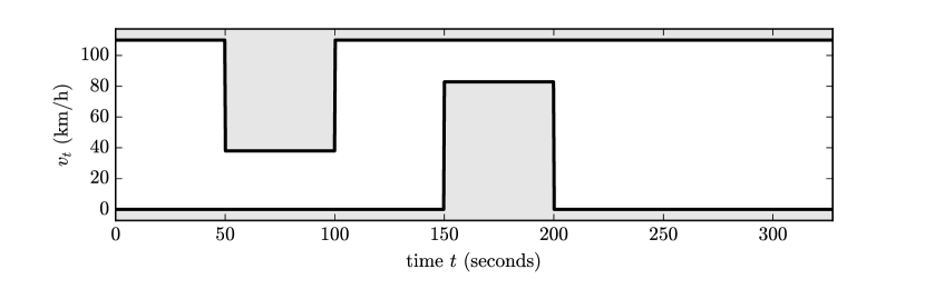
Figure 1: The velocity limits $v_{t}^{\rm min}$ and $v_{t}^{\rm max}$ over time.

parameter	value
$m$	$1500$ kg
$E^{\rm init}$	$4000$ kJ
$E^{\rm min}$	$0$ kJ
$E^{\rm max}$	$4000$ kJ
$x^{\rm init}$	$0$ m
$v^{\rm init}$	$0$ m
$\rho$	$1.22$ $\rm kg/m^{3}$
$C_{D}$	$0.35$
$A$	$2.3$ $\rm m^{2}$
$C^{\rm rr}$	$0.005$ $\rm kN/(m/s)$
$x^{\rm end}$	$5000$ m

Table 1: Parameter values.

To obtain a numerical solution, problem (8) was first discretized in time by dividing the interval $[0,T]$ into $1001$ discrete points. It was solved using CVXPY [DB16], with backend solver ECOS [DCB13].

Pareto curve.

The trade-off between the total energy consumed and the travel time is depicted in figure 2. The shaded region is the set of possible pairs $(E^{\rm init}-E_{T},T)$ of energy consumption and travel time corresponding to feasible trajectories of (8). The Pareto curve is shown as a bold line. Trajectories correspending to any point on this line can be computed by fixing $T$ and solving (8). The three colored crosses are specific Pareto-optimal trajectories, which are shown in detail in figure 3.

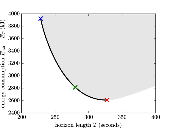
Figure 2: The Pareto optimal curve trading off energy consumption and travel time. The blue and red crosses correspond to the minimum-time and minimum-energy trajectories, and the green cross corresponds to a compromise between these two.

Sample trajectories.

We now describe in detail the three trajectories shown in figure 3. We begin by describing the trajectory shown in green, found by solving (8) with a travel time of $T=280$ seconds. The trajectory begins with acceleration at the maximal rate $a_{t}^{\rm max}$; the drive power is then decreased, until it reaches zero, and the vehicle coasts until the upper speed limit is reached during time period $t=50$ seconds. At this point the vehicle brakes, then supplies constant power to maintain speed at the speed limit. After the speed limit ends ($t=100$ s), the vehicle accelerates to a roughly constant “cruising speed” of around $80$ $\rm km/h$. Of particular interest is the existence of a coasting interval during the last $50$ seconds, during which the drive power is zero as the vehicle coasts to the desired displacement. This is a solution to the apparent dilemma that a positive vehicle speed is required to reach the desired displacement, yet any leftover positive kinetic energy at this point can be considered wasted energy. (One might argue that this leftover kinetic energy could have been put to better use accelerating the vehicle earlier on; evidently, this argument is false.)

The trajectory shown in blue is the minimum-time trajectory, i.e., it is the smallest value of $T$ for which (8) is feasible. Note that this control depletes the internal energy exactly as the desired displacement is reached. The trajectory often accelerates aggressively, using a substantial amount of power to get to a high speed quickly. Even so, the minimum-time trajectory has a coasting period that begins around $t=210$ seconds and lasts until the end of the time period.

Finally, in red, we see the minimum-energy trajectory, which is found by computing the value of $T$ that maximizes the optimal value of problem (8). As one might expect, the speed is kept lower than for the previous two trajectories, which both decreases the amount of energy required to accelerate the vehicle, and the power lost to drag. However, the minimum-energy trajectory still reaches the desired displacement in a finite amount of time. This is because our model assumes that the engine is turned on during the interval $[0,T]$, and idling incurs a power loss of $\gamma$. Therefore, the minimum-energy control is motivated not to waste any time in reaching the goal, i.e., being fast also helps reduce wasted energy.

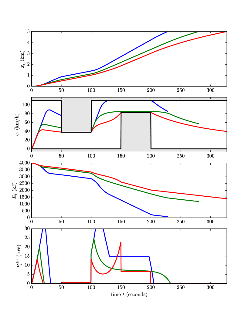
Figure 3: Three optimal trajectories, obtained by solving (8) for different values of $T$.

5 Conclusions

We used a simple optimization model to capture the trade-off between vehicle energy consumption and travel time. Several interesting extensions are possible, especially for different drivetrain architectures, and our formulation easily accommodates drivetrain models formulated in terms of energy and power. Modeling a solar car is a particularly simple extension, which involves adding a time-varying prediction of generated solar power into the internal energy dynamics equation (5). Another extension involves adding a time-dependent disturbance to the kinetic energy dynamics (5), which could model the predicted power loss (or gain) from traversing hilly terrain.

References

- [BV04] S. Boyd and L. Vandenberghe. Convex Optimization. Cambridge University Press, 2004.
- [CPDB13] E. Chu, N. Parikh, A. Domahidi, and S. Boyd. Code generation for embedded second-order cone programming. In Proc. of the 2013 European Control Conference, pages 1547–1552, 2013.
- [DB16] S. Diamond and S. Boyd. CVXPY: A Python-embedded modeling language for convex optimization. Journal of Machine Learning Research, 17(83):1–5, 2016.
- [DCB13] A. Domahidi, E. Chu, and S. Boyd. ECOS: An SOCP solver for embedded systems. In Proceedings of the 12th European Control Conference, pages 3071–3076. IEEE, 2013.
- [LB14] T. Lipp and S. Boyd. Minimum-time speed optimisation over a fixed path. International Journal of Control, 87(6):1297–1311, 2014.
- [MB10] J. Mattingley and S. Boyd. Automatic code generation for real-time convex optimization. In Y. Eldar and D. Palomar, editors, Convex Optimization in Signal Processing and Communications, pages 1–41. Cambridge University Press, 2010.
- [OSB13] B. O’Donoghue, G. Stathopoulos, and S. Boyd. A splitting method for optimal control. IEEE Transactions on Control Systems Technology, 21(6):2432–2442, Nov 2013.
- [PB14] A. Panday and H. O. Bansal. A review of optimal energy management strategies for hybrid electric vehicle. International Journal of Vehicular Technology, 2014, 2014.
- [TB00] E. D. Tate and S. Boyd. Finding ultimate limits of performance for hybrid electric vehicles. Technical report, SAE Technical Paper, 2000.
- [UMTB18] S. Uebel, N. Murgovski, C. Tempelhahn, and B. Bäker. Optimal energy management and velocity control of hybrid electric vehicles. IEEE Transactions on Vehicular Technology, 67(1):327–337, 2018.
- [WB10] Y. Wang and S. Boyd. Fast model predictive control using online optimization. IEEE Transactions on Control Systems Technology, 18(2):267–278, 2010.