Effect of the degree of an initial mutant in Moran processes in structured populations

Abstract

We study the effect of the mutant’s degree on the fixation probability, extinction and fixation times, in the Moran process on Erdös-Rényi and Barabási-Albert graphs. We performed stochastic simulations and use mean-field type approximations to obtain analytical formulas. We showed that the initial placement of a mutant has a significant impact on the fixation probability and extinction time, while it has no effect on the fixation time. In both types of graphs, an increase in the degree of a initial mutant results in a decreased fixation probability and a shorter time to extinction.

I Introduction

Extinction and fixation of phenotypes and behaviors in animal and human populations are important features of evolutionary processes. The classical model here is the Moran process in populations of fixed finite sizes, consisting of individuals equipped with one of two phenotypes [1]. Namely, an individual is chosen proportional to her fitness (which can be constant or resulting from payoffs received in game competitions) gives birth to an offspring who inherits her phenotype and replaces a randomly chosen individual. Such a birth-death process is a Markov chain with two absorbing states: homogeneous populations with only one strategy present. Now, one may wish to compute a fixation probability and expected fixation and extinction times of mutants who appeared in a population. We are interested especially in the fixation probability of a strategy held by one mutant. If fitness of a mutant is the same as of residents, then obviously such a fixation probability is equal to $1/N$, where $N$ is the size of the population. On the other hand, if fitness of mutants and residents are different, then if the above fixation probability is bigger than $1/N$, we may say that evolution favors the mutant’s phenotype.

The Moran process in well-mixed populations with individuals/players, whose fitness come from payoffs in game competitions, was analyzed in [2, 3]. The authors considered a Stag-hunt type game with two strategies and two pure Nash equilibria asymptotically stable in the replicator dynamics and an unstable mixed Nash equilibrium. They derived the so-called $1/3$ rule which states that a strategy is favored by evolution if the frequency of that strategy is less than $1/3$ in the mixed Nash equilibrium. The $1/3$ law was rederived and generalized in other evolutionary processes by means of potential functions in one-dimensional discrete dynamics in [4].

In well-mixed populations, payoffs of players are expected payoffs with probabilities of meeting various players depending on the current structure of a population. In spatial processes (evolutionary games), individuals are placed on vertices of networks/graphs and their payoffs are sums of payoffs resulting from games with their neighbors [5, 6, 7]. Accordingly, in Moran processes on graphs, offspring replace neighbors of ancestors. Theoretical studies have shown that the structure of the population can have a significant impact on the evolutionary dynamics and can affect fixation probability and fixation time [8, 9, 10, 11, 12, 13, 14, 15, 16]. For example, some studies have investigated the impact of degree heterogeneity on fixation probability and fixation time [12, 13]. Other studies have examined the role of a modular structure, where the population is divided into distinct modules or communities, and found that modular structure can change the fixation time and probability of a mutant [14, 15]. In [16] it was shown how the probability of fixation behaves concerning the complexity parameter. Specifically, they investigated the effect of the scale-free exponent for the scale-free network and the rewiring probability for the small-world network on fixation probability. Another paper demonstrated that the presence of a small number of nodes with high degrees prolongs the fixation time, whereas the presence of a few shortcuts reduces the fixation time [17]. Some studies have explored a novel method that involves a Markov chain corresponding to the process to determine fixation time in networks with a small number of nodes and simple structure [18]. In [19], the authors have devised an approach using a mean-field technique for more intricate structured populations, such as scale-free and small-world graphs.

Here we discuss the Moran process on random Erdös-Rényi [20] and Barabási-Albert [21, 22] graphs. We assume that the fitness of mutant is equal to $r>1$ and $1$ for residents (no game competitions are included in our models). More specifically, we studied dependence of fixation and extinction probabilities and expected times of fixation and extinction on a graph degree of an initial mutant. The effect of a placement of an initial mutant was studied in [23]. The authors derived a useful analytical approximation of fixation probability as a function on the degree of the initial mutant for some simple graphs. Their findings revealed that initial mutants with fewer connections had a greater advantage, resulting in a higher probability of fixation. However, the influence of an initial mutant on fixation (or extinction) probability and time in more complex graphs, such as scale-free graphs, has not been studied yet.

We performed stochastic simulations and derived analytical formulas based on mean-field and pair-approximation ideas applied to random Erdös-Rényi and Barabási-Albert graphs. We showed that the initial placement of a mutant has a significant impact on the fixation probability and extinction time, while the degree of the initial mutant has no effect on the fixation time. In both types of graphs, an increase in the degree of the initial mutant results in a decreased probability of the mutant taking over the entire population and a shorter time to extinction. In the two graphs with the same size and average vertex degree, for an initial mutant with the same degree, the fixation probability in Erdös-Rényi graph is higher than in Barabási-Albert one. However, due to the presence of hubs, the average fixation probability in Barabási-Albert graph is higher.

In Section II, we present our model - a Markov chain of the Moran process on graphs. In Section III, we present results of stochastic simulations and derive analytical results. Further analysis of extincion time is contained in Section IV. Discussion follows in Section V.

II Models and methods

We will study here the Moran process on two random graphs, the Erdös-Rényi (ER) [20] and the scale-free Barabási-Albert (BA) one [21, 22]. We build the ER graph by putting with probability $p$ an edge between every pair of $N=500$ vertices. It follows that the average degree of vertices (the average number of neighbors) is equal to $\alpha=p(N-1).$ The BA network is built by the preferential attachment procedure. We start with $m_{o}$ fully connected vertices and then we add $N-m_{o}$ vertices, each time connecting them with $m$ already available vertices with probabilities proportional to their degrees. If $m_{o}=\alpha+1$ and $m=\alpha/2$, then we get a graph with the average degree equal to $\alpha$. It is known that such a graph is scale-free with the probability distribution of degrees given by $p(k)\sim k^{-3}$ [21, 22, 24].

Individuals - mutants with a constant fitness $r$ and residents with a constant fitness $1$ - are located on vertices of a graph. At every time step of the process, an individual is chosen with a probability proportional to her fitness and then gives birth to an offspring who inherits her phenotype and replaces a randomly chosen individual. Such a Markov chain with ${N}^{2}$ states has two absorbing ones: homogeneous populations with only one type of individuals present. We start our process with one mutant in the population of residents. We are interested in the fixation probability, expected time to fixation and to extinction of mutants, denoted respectively by $\rho^{f}_{1},e^{f}_{i}$ , and $e^{e}_{1}$. To find such quantities, we performed stochastic simulations.

We simulate the Moran process on graphs with $N=500$ vertices. For avery $k$, we randomly place an initial mutant on one of the nodes of the degree k and perform 10,000 Monte-Carlo simulations untill the population reaches one of two absorbing states. To get fixation probability, we devide the number of times the process ends in the all-mutant state by 10,000. Finally we calculate an average fixation (extinction) time for some chosen k’s.

It is impossible to get rigorous analytical expressions for fixation and extinction probabilities and times for Moran procesees on graphs. Situation is much simpler in well-mixed populations. Then the Moran process becomes a Markov chain with $N+1$ states corresponding to the number of mutants or more precisely, a random walk on $\{0,...,N\}$ with state-dependent probabilities of moving to the right, $p_{i\rightarrow i+1}$, to the left, $p_{i\rightarrow i-1}$, and not moving, $1-p_{i\rightarrow i+1}-p_{i\rightarrow i-1}$. Such a model is well-known in the context of a gambler’s ruin problem. It is easy to see that here we have that $p_{i\rightarrow i+1}=rp_{i\rightarrow i-1}$. For the fixation probability starting from $i$ mutants, one can then get that

$$\rho^{f}_{i}=\frac{1-\frac{1}{r^{i}}}{1-\frac{1}{r^{N}}}.$$ (1)

For the fixation probability on graphs, to take into account a degree of an initial mutant, we derive some approximate expressions for transition probabilities up to $3$ mutants and then use the elementary conditional probability formula and the fixation probability $\rho^{f}_{3}$ from (1) to obtain analytic expression for the fixation probability as a function a degree of an initial mutant. In that way we passed from the full Markov chain with $2^{N}$ states to one with $N+1$ states corresponding to the number of mutants.

In the following section, we derive analytic exprsessions for the fixation probability and expected extinction time, and compare them with results of stochastic simulations.

III Results

III.1 Fixation probability

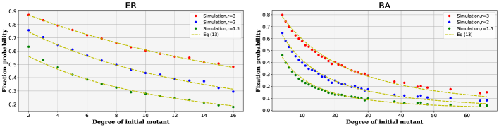
Figure 1: (color online) Fixation probability as a function of a degree of an initial mutant for three fitness values: 3, 2, 1.5 in ER and BA graphs with the size of 500 and the average degree of 8.

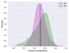
Figure 2: Distribution of fixation probabilities with respect to a degree of an initial mutants for ER and BA graphs with the size of $500$ and the average degree of $8$. The fitness is $2$. Dash lines show the average fixation probability.

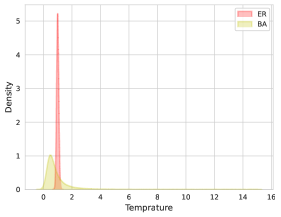
Figure 3: The distribution of temperature in ER and BA graphs. The node temperature is simply defined as the inverse of the degree of all nodes leading to that node.

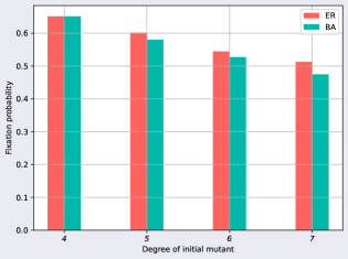
Figure 4: Fixation probability for different initial mutants with the same degree in ER and BA graphs. The size of the graph is $500$ with the average degree of $8$ and $r=2$.

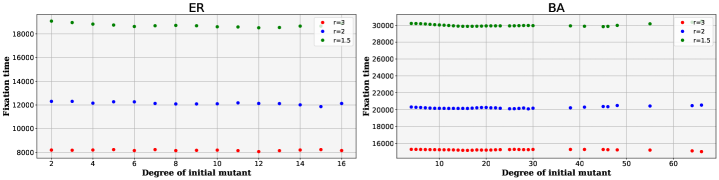
Figure 5: (color online) Fixation time as a function of the degree of an initial mutant for three fitness values, 3, 2, 1.5 in ER and BA graphs with the size of 500 and the average degree of 8.

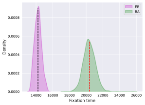
Figure 6: Distribution of fixation times with respect to a degree of an initial mutants for ER and BA graphs with the size of $500$ and the average degree of $8$. The fitness is $2$. Dash lines show the average fixation time.

Let $\rho^{f}_{i}$ be the fixation probability when there are $i$ mutants in the population and we denote by $P_{i\rightarrow j}$ the probability of the transtion from the state $i$ to the state $j$; of course, for our Moran process, transition probabilities are non-zero only for $|i-j|\leq 1$. From the total probability formula we get

$$\rho^{f}_{1}=P_{1\rightarrow 1}\rho^{f}_{1}+P_{1\rightarrow 2}\rho^{f}_{2}.$$ (2)

$$\rho^{f}_{2}=P_{2\rightarrow 1}\rho^{f}_{1}+P_{2\rightarrow 2}\rho^{f}_{2}+P_{2\rightarrow 3}\rho^{f}_{3}.$$ (3)

We substitute (3) to (2) and get

$$\rho^{f}_{1}=\dfrac{P_{1\rightarrow 2}P_{2\rightarrow 3}}{(P_{1\rightarrow 2}+P_{1\rightarrow 0})(P_{2\rightarrow 1}+P_{2\rightarrow 3})-P_{1\rightarrow 2}P_{2\rightarrow 1}}\rho^{f}_{3}$$ (4)

For the number of mutants to increase from $1$ to $2$, the mutant should be chosen for reproduction, hence

$$P_{1\rightarrow 2}=\frac{r}{N+r-1}.$$ (5)

For the number of mutants to decrease from $1$ to $0$, a resident from the mutant’s neighborhood with degree $k$ must be selected and its offspring placed in the mutant’s location, hence,

$$P_{1\rightarrow 0}=\sum_{k^{{}^{\prime}}}\frac{k}{r+N-1}\frac{1}{{k^{{}^{\prime}}}}{{\rho}^{{}^{\prime}}(k^{{}^{\prime}})},$$ (6)

where $k^{\prime}$ is the degree of the selected resident and ${{\rho}^{{}^{\prime}}(k^{{}^{\prime}})}$ is the degree distribution of neighbors of the mutant.

The distribution ${{\rho}^{{}^{\prime}}(k^{{}^{\prime}})}$ of degrees of a node which is connected to a given node can be approximated by $\frac{k^{{}^{\prime}}\rho(k^{{}^{\prime}})}{<k>}$, where $\rho(k^{{}^{\prime}})$ is the degree distribution in the graph [25, 26]. Therefore

$$P_{1\rightarrow 0}=\frac{k}{r+N-1}\frac{1}{<k>}.$$ (7)

Now we have to calculate $P_{2\rightarrow 1}$. For this transition, one of the resident neighbors of two mutants must be chosen for the reproduction and replace the mutant. One of them is the first mutant with a degree of $k$, while the other is a previously mutated node with a degree of $k^{{}^{\prime}}$. We have the following formulas:

$$\begin{split}P_{2\rightarrow 1}=\sum_{k^{{}^{\prime}}}\frac{k-1}{2r+N-2}\frac{1}{{k^{{}^{\prime}}}}\frac{k^{{}^{\prime}}\rho(k^{{}^{\prime}})}{<k>}+\hskip 40.0pt\\ \sum_{k^{{}^{\prime}}}\sum_{k^{"}}\frac{k^{\prime}-1}{2r+N-2}\frac{1}{{k^{"}}}\frac{k^{{}^{\prime}}\rho(k^{{}^{\prime}})}{<k>}\frac{k^{"}\rho(k^{"})}{<k>}\end{split}$$ (8)

and after some simplifications

$$P_{2\rightarrow 1}=\dfrac{1}{2r+N-2}\dfrac{1}{<k>}(k+\frac{<k^{2}>}{<k>}-2).$$ (9)

In the the same way we obtain $P_{2\rightarrow 3}$,

$$P_{2\rightarrow 3}=\frac{r}{2r+N-2}\frac{k-1}{k}+\sum_{k^{{}^{\prime}}}\frac{r}{2r+N-2}\frac{k^{{}^{\prime}}-1}{k^{{}^{\prime}}}\frac{k^{{}^{\prime}}\rho(k^{{}^{\prime}})}{<k>}$$ (10)

and after some simplifications we have,

$$P_{2\rightarrow 3}=\dfrac{r}{2r+N-2}(\frac{k-1}{k}-\frac{1}{<k>}+1)$$ (11)

This allow us to rewrite (4) as follows:

$$\rho^{f}_{1}=\dfrac{{<k>}^{2}r^{2}(2-\frac{1}{k}-\frac{1}{<k>})}{(r<k>+k)(r<k>(2-\frac{1}{k}-\frac{1}{<k>})+(k-2+\frac{<k^{2}>}{<k>}))-r<k>(k-2+\frac{<k^{2}>}{<k>})}\rho^{f}_{3}.$$ (12)

Now we assume that the effect of an initial mutant is limited to transitions from one-mutant population to two-mutant population and also from two mutants to three mutants. Hence we take $\rho^{f}_{3}$ from (1) and get

$$\rho^{f}_{1}=\dfrac{{<k>}^{2}r^{2}(2-\frac{1}{k}-\frac{1}{<k>})}{(r<k>+k)(r<k>(2-\frac{1}{k}-\frac{1}{<k>})+(k-2+\frac{<k^{2}>}{<k>}))-r<k>(k-2+\frac{<k^{2}>}{<k>})}\dfrac{1-\frac{1}{r^{3}}}{1-\frac{1}{r^{N}}}.$$ (13)

To determine the fixation probability of mutants with degree $k$, we need to use (13), which requires the knowledge of the average degree $<k>$ and the second moment $<k^{2}>$ of the graph. For the Erdös-Rényi graph with the binomial degree distribution, the average degree is equal to $<k>=(N-1)p$, and the second moment $<k^{2}>=<k>(<k>(1-1/(N-1))+1)$. For the Barab’asi-Albert graph, the degree distribution follows a power-law, resulting in an average degree of $<k>=2m$ and $<k^{2}>\equiv<k>^{2}logN/4$ [27].

Fig.1 depicts the outcomes of both the analytical and computer simulation approaches for three diverse fitness values. Both figures exhibit a decrease in the probability of fixation when the initial mutant’s degree increases. As the degree of the initial mutant increases, it becomes more probable that one of its resident neighbors replaces it. Hence, vertices with a lower number of connections have a higher chance of remaining and progressing toward fixation. In the BA graph, the degree distribution follows a power law, which means that there are a few nodes with very high degrees and many nodes with low degrees. Consequently, in the BA graph, there may be initial nodes with a high probability of fixation, mainly those with low degrees, and others with very low fixation probabilities, mainly those with high degrees, in contrast to the ER graph where the probability of fixation is more uniform across nodes.

In Fig.2, we can observe the distribution of fixation probabilities for different initial mutants with various degrees in both graphs of the same size, average degree, and fitness. In ER graphs, fixation probabilities for all vertices are approximately distributed symmetrically around the average fixation probability. However, in the BA graph, the distribution is asymmetric. Moreover, we see that for $r=2$, the average fixation probability in the ER graph is approximately $0.5$ which is the fixation probability in a well-mixed population, while this value is slightly higher in the BA graph.

This can be understood on the basis of a concept of the so-called temperature vertex which is defined as the sum of the inverses of degrees of all neighbors of a given vertex. It was proven in [28] that for graphs for which all vertices have the same temperature, the so-called isothermal graphs, the average fixation probability is equal to the one in well-mixed populations.

Fig.3 displays the temperature distribution for both graphs with the size of 500 and an average degree of 8. The ER graph exhibits a peak at 1, indicating that nearly all nodes have the same temperature. In contrast to the ER graph, the BA graph’s vertices have significantly different temperatures. While there are many vertices with small degrees, leading to higher fixation probabilities, there are only a few vertices with large degrees, leading to low fixation probabilities. Consequently, the average fixation probability in the BA graph is higher than in well-mixed populations and ER graphs.

In Fig.4, we present the fixation probability for an equal degree of initial placement for both graphs. As shown, the fixation probability in case when the popolatiion hasone mutant in the same degree in both graphs, is slightly higher for the ER graph. However, this does not contradict the observation that the average fixation probability is higher in the BA network. While it is true that the fixation probability for initial mutants with the same degree is higher in ER graphs, there are more nodes with a low degree in BA graphs, which have a higher fixation probability thanin ER graphs. As a result, the average fixation probability in the BA graph is greater than that in the ER graph.

III.2 Fixation Time

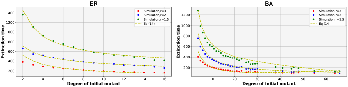
Figure 7: (color online) Extinction time as a function of a degree of an initial mutant for three fitness values: 3, 2, 1.5 in ER and BA graphs with the size of 500 and average degree of 8.

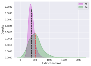
Figure 8: Distribution of extinction times with respect to a degree of an initial mutants in both graphs with the size of $500$ and the average degree of $8$. The fitness is $2$. The dash lines show the average extinction times.

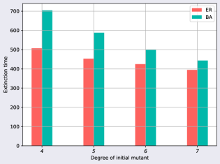
Figure 9: Extinction time for different initial mutants with the same degree in both networks. The size of the networks is $500$, the average degree $8$ and $r=2$.

Fig.5 shows that there is no difference in fixation times for various degrees of an initial mutant. The distribution of fixation times is shown in Fig.6. We can see that the fixation times are distributed symmetrically around the average fixation time in both graphs. One notable point is that the average fixation time in the BA graph is higher than in EA.

III.3 Extinction Time

To derive an analytical expression for the average extinction time we use a well-known technique described in [18, 19], details of caulations are contained in the Appendix. The time to extinction starting from one mutant is given by the following formula,

$$t^{e}_{1}=\frac{1}{\rho^{e}_{1}}\sum_{j=1}^{N-1}\rho^{e}_{j}F_{1j}=\frac{1}{1-\rho^{f}_{1}}\sum_{j=1}^{N-1}(1-\rho^{f}_{j})F_{1j},$$ (14)

where $\rho^{f}_{1}$ is given in (13) and $\rho^{f}_{j}$ for $j>1$ in (1). Here, $\rho_{j}^{e}=1-\rho_{j}^{f}$ is the extinction probability. $F_{1j}$ are given in (23) in the Appendix, they are the numbers of times the process moves from the state 1 to the state j before reaching an absorbing state. Values of $F_{1j}$ depend on graphs.

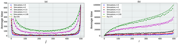
Figure 10: (color online) a) expected number of times the process which started with one mutant passes through the state with j mutants before reaching fixation, $t^{f}_{1,j}$, eq. (15) and b) the average time required until the number of mutants reaches $j$, $T^{f}_{i}$, eq. (17), for different values of $r$ in ER graph with $N=500$ and average degree of $8$.

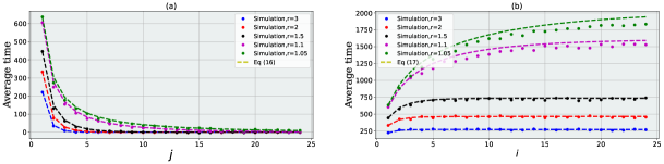
Figure 11: (color online) a) expected number of times the process which started with one mutant passes through the state with j mutants before reaching extinction, $t^{e}_{1,j}$, eq. (16) and b) the verage time required until the number of mutants reaches $j$, $T^{e}_{i}$, eq. (17), for different values of $r$ in ER graph with $N=500$ and average degree of $8$.

We have presented results of computer simulations and our analytical approach in Fig.7. It appears that extinction time and initial mutant degree are inversely related and that as the initial mutant degree increases, extinction time decreases. Essentially, as the initial mutant degree increases, it becomes more likely to select one of its neighbors to replace it. As a result, mutants with higher degrees are more likely to be wiped out in a short period of time. In the BA graph, for two initial mutants with a large difference in degree, we have completely different extinction times due to the average degree of the network. It is worth noting that for vertices with high degrees, the extinction time is almost the same for all values of r. In other words, if the process starts from a hub regardless of $r$, it will soon become extinct. In Fig.8, we can see the distribution of extinction times for both graphs. In the ER graph, extinction times are distributed around an average time, while in the BA graph, the distribution is more extended. ER graphs exhibit lower average extinction times than BA graphs.

As demonstrated in Fig.9, the extinction time for various initial mutants with the equivalent degrees is presented. observe that for initial mutants with the equal number of connections, the one in the BA graph exhibits a longer extinction time.

IV Fixation and extinction times - discussion

Here we examine in more detail the evolution of a population starting with one mutant. Fig.10 and Fig.11 show the path to extinction and fixation of mutant in ER graph with a size of $500$ and an average degree of 8. We derived approximate formulas for expected number of times the process which started from $i$ mutants, passes through the state with $j$ mutants before reaching fixation and extinction time respectively (details of derivation are given the Appendix),

$$t^{f}_{i,j}=\begin{cases}\dfrac{{(r^{j}-1)}^{2}(r^{N-i}-1)r^{i-j}}{(r-1)(r^{N}-1)(r^{i}-1)\frac{j}{N-i+rj}\frac{(N-j)(p-\frac{2}{N})}{Np}}\hskip 5.0ptj\leq i\\[15.0pt] \dfrac{(r^{N-j}-1)(r^{j}-1)}{(r-1)(r^{N}-1)\frac{j}{N-i+rj}\frac{(N-j)(p-\frac{2}{N})}{Np}}\hskip 39.0ptj>i\end{cases}$$ (15)

$$t^{e}_{i,j}=\begin{cases}\dfrac{{(r^{j}-1)}(r^{N-i}-1)(r^{N}-r^{j})r^{i-j}}{(r-1)(r^{N}-1)(r^{N}-r^{i})\frac{j}{N-i+rj}\frac{(N-j)(p-\frac{2}{N})}{Np}}\hskip 5.0ptj\leq i\\[15.0pt] \dfrac{(r^{N}-r^{j})(r^{N-j}-1)(r^{i}-1)}{(r-1)(r^{N}-1)(r^{N}-r^{i})\frac{j}{N-i+rj}\frac{(N-j)(p-\frac{2}{N})}{Np}}\hskip 5.0ptj>i\end{cases}$$ (16)

We have perfomed stochatic simulations to see how accurate are analytical formulas.

Panels (a) in Fig.10 and Fig.11 illustrate the number of times there are $i$ mutants in the population starting with one mutant, while panels (b) demonstrate how long it takes a single mutant to take over $i$ nodes in a network ($T_{i}$) before extinction and fixation respectively. For a single mutant to be fixed, the Moran process must pass from the state with $i$ mutants. Thus, $T_{i}$ is the time needed for a single mutant to be fixed minus the time needed for $i$ mutants to be fixed. Therefore we have,

$$\begin{split}T^{f}_{i}=t^{f}_{1}-t^{f}_{i}=\sum_{j=1}^{N-1}t^{f}_{1,j}-\sum_{j=1}^{N-1}t^{f}_{i,j},\\ T^{e}_{i}=t^{e}_{1}-t^{e}_{i}=\sum_{j=1}^{N-1}t^{e}_{1,j}-\sum_{j=1}^{N-1}t^{e}_{i,j}.\end{split}$$ (17)

We observe that the process before extinction spend most of time in states with few mutants. This means that during the process of the extinction of mutants, a few vertices get mutated and if the number of mutants increases, there is a higher chance of them to be fixed. Therefore, the initial placement of mutants plays an important role in the extinction of mutants. For fixation, unlike extinction, the beginning and the end of the process can have a significant impact on the time fixation time. At the beginning of the process when few mutants are available, the probability of choosing them to reproduce is low, so it takes a long time for mutants to increase their number. Furthermore, with fewer residents in the population, it takes longer time to replace them with one of the mutants’ offspring at the end of the process. Hence it doesn’t matter where the mutant is initially placed because the start and end of the process are equally important for fixation time.

We observe that our analytical expressions are less accurate for smaller values of $r$ and are becoming better as $r$ increases. We assumed that the initial mutant degree influences only the probability of transition between one to two and two to three mutants. However, there is a possibility that the number of mutants increases and then decreases again to one. Hence, the mutant may be different from the starting mutant, leading to an error in our approximation. For large $r$, there is a low probability that the number of mutants will decrease to one. Therefore, when there are more mutants, they are more likely to increase rather than decrease their number. Consequently, our approximation is better for larger $r$.

V Discussion

To summarize, we examined the impact of the degree of an initial mutant on the fixation probability and fixation and extinction times in the Moran process in structured populations. We performed computer simulations and derived approximate analytical expressions.

We showed that the fixation probability greatly depends on the vertex degree at which the mutant is introduced. Increasing the degree of the initial mutant makes it more likely for the mutant to be replaced by one of its neighbors. There was no correlation between the degree of the initial mutant and the time it took for the mutant to take over the entire population. The fixation process depends on the entire population, not on the first mutant. We found that, unlike fixation time, extinction time significantly depends on the degree of the first mutant - a mutant with few connections needs more time to become extinct. Furthermore, we observed that the extinction time for an initial mutant with a small degree is significantly influenced by its fitness, but as the degree of the first mutant increases, extinction times become independent on the fitness value.

It is important to study the impact of the initial mutant’s degree on the fixation probability and fixation and extinction times in frequency-dependent Moran processes of spatial evolutionary games, where fitness is derived from game competitions.

Acknowledgments: This project has received funding from the European Union’s Horizon 2020 research and innovation programme under the Marie Skłodowska-Curie grant agreement No 955708. Computer simulations were made with the support of the Interdisciplinary Center for Mathematical and Computational Modeling of the University of Warsaw (ICM UW) under the computational grant No g91-1417.

VI Appendix

We consider here a reduced Markov chain for the Moran process on the graph with $N+1$ states representing the number $i$ mutant in the population. The transition matrix can be then written as follows:

$$P_{ij}=p_{i\rightarrow i+1}\delta_{i+1,j}+p_{i\rightarrow i-1}\delta_{i-1,j}+q_{i}\delta_{i,j}\;.$$ (18)

where $q_{i}=1-p_{i\rightarrow i+1}-p_{i\rightarrow i-1}$.

Our Markov chain has two absorbing states: $i=0$ and $i=N$. To calculate absorbing probabilities and expected absorbing times we use the general method described in [29]. We rewrite the transition matrix as follows:

$$P=\begin{pmatrix}Q&R\\ 0&I\end{pmatrix},$$ (19)

where $Q$ contains transition probabilities between transiient states and $R$ contains transition probabilities from transient states to absorbing ones, and $I$ is the identity matrix. $F=(I-Q)^{-1}$ is called the fundamental matrix. It can be shown that $F_{ij}$ are expected number of times the process which started from $i$ mutants, passes through the state with $j$ mutants before reaching one of the absorbing states time. Then it follows that absorption expected times are given by summations,

$$t_{i}=\sum_{j=1}^{N-1}F_{ij}.$$ (20)

Expected number of times the process which started from $i$ mutants, passes through the state with $j$ mutants before reaching fixation and extinction time can be written as follows [18],

$$\begin{array}[]{rl}t^{f}_{i,j}=\frac{\rho^{f}_{j}}{\rho^{f}_{i}}F_{ij},\\ t^{e}_{i,j}=\frac{\rho^{e}_{j}}{\rho^{e}_{i}}F_{ij}.\end{array}$$ (21)

Hence expected fixation and extinction times are given by the following expressions,

$$\begin{array}[]{rl}t^{f}_{i}=\sum_{j=1}^{N-1}\frac{\rho^{f}_{j}}{\rho^{f}_{i}}F_{ij},\\ t^{e}_{i}=\sum_{j=1}^{N-1}\frac{\rho^{e}_{j}}{\rho^{e}_{i}}F_{ij}.\end{array}$$ (22)

Now we turn our attention to graphs. It can be shown that if the Moran process on a graph satisfies the condition $p_{i\rightarrow i+1}=rp_{i\rightarrow i-1}$, then we have [19],

$$F_{ij}=\begin{cases}\frac{(r^{j}-1)(r^{N-i}-1)}{p_{j\rightarrow j-1}(r-1)(r^{N}-1)},j\leq i\\[15.0pt] \frac{r^{j-i}(r^{i}-1)(r^{N-j}-1)}{p_{j\rightarrow j-1}(r-1)(r^{N}-1)},i<j\end{cases}$$ (23)

The authors of [19] used mean-field techniques and argue that $p_{i\rightarrow i+1}=rp_{i\rightarrow i-1}$ is a good approximation for Erdös-Rényi and Barabási-Albert graphs. We present here their arguments and results.

• Erdös-Rényi graph (ER)

  In the ER graph with $N$ vertices and $j$ mutants, the probability of a mutant being selected for the reproduction is given by $\frac{rj}{rj+N-j}$. Although it may seem that this mutant would have $(N-j)p$ residents in its neighborhood, the population of mutants tends to form cluster, making it likely for a selected mutant to have at least two mutant neighbors. Thus, the probability of a selected mutant being connected to a resident is approximately $(p-\frac{2}{N})$, and the average number of residents connected to a selected mutant is ($N-j)(p-\frac{2}{N})$. Then

  $$p_{j\rightarrow j+1}=rp_{j\rightarrow j-1}=\frac{rj}{N-i+rj}\frac{(N-j)(p-\frac{2}{N})}{(N-1)p}.$$ (24)

• Barabási-Albert graph (BA)

  Here again, the probability for a mutant to be chosen for the reproduction is $\dfrac{rj}{rj+N-j}$ For a state with $j$ mutants, $I_{j}$ represents the average number of edges that connect different species, also known as interface edges. On average, each mutant (resident) has $<k>$ connections, and $\frac{I_{j}}{j}$ ($\frac{I_{j}}{(N-j)}$) interface edges. As a result, the probability for a mutant (resident) offspring to replace one of its resident (mutant) neighbors is $\frac{\frac{I_{j}}{j}}{m}$ ($\frac{\frac{I_{j}}{(N-j)}}{m}$). This leads to the conclusion that $\lambda_{i}$ and $\mu_{i}$ can be expressed as:

  $$p_{j\rightarrow j+1}=rp_{j\rightarrow j-1}=\frac{rI_{j}}{<k>(N-j+rj)}.$$ (25)

  In order to find $I_{j}$ when there are $i$ mutants, it is evident that every resident node has at least $m$ edges and an average of $\frac{I_{j}}{N-j}$ interface edges. If one resident is changed to a mutant, the number of mutants increases by 1. Therefore, we can obtain a recursive relationship for the number of interface edges as follows:

  $$I_{j+1}=I_{j}+m-\dfrac{I_{j}}{N-j}.$$ (26)

  Assuming $I_{0}=0$ we have:

  $$I_{j}=m\sum_{i=1}^{j}\frac{N-j}{N-i}.$$ (27)

References

- [1] P. A. P. Moran. Random processes in genetics, Math. Proc. Cambridge Philos. Soc. 54, 60–71 (1958).
- [2] M. A. Nowak, A. Sasaki, C. Taylor, and D. Fudenberg, Emergence of cooperation and evolutionary stability in infinite populations, Nature 428, 646-650 (2004).
- [3] H. Ohtsuki, P. Bordalo, and M. A. Nowak, The one-third law of evolutionary dynamics, J. Theor. Biol. 249, 289-295 (2007).
- [4] P. Nałȩcz-Jawecki and J. Miȩkisz, Mean-potential law in evolutionary games, Phys. Rev. Lett. 120, 028101 (2018).
- [5] M. A. Nowak and R. M. May, Evolutionary games and spatial chaos, Nature 359, 826-829 (1992).
- [6] G. Szabó and G. Fáth, Evolutionary games on graphs, Phys. Rep. 446, 97-216 (2007).
- [7] J. Miȩkisz, Evolutionary game theory and population dynamics, in Multiscale Problems in the Life Sciences, From Microscopic to Macroscopic, V. Capasso and M. Lachowicz (eds.), Lecture Notes in Mathematics 1940, 269-316 (2008).
- [8] H. Ohtsuki, and M. A. Nowak, Evolutionary games on cycles, Proc. R. Soc. B Biol. Sci. 273, 2249-2256 (2006).
- [9] A. Traulsen and M. A. Nowak, Evolution of cooperation by multilevel selection, Proc. Natl. Acad. Sci. U.S.A 103, 10952-10955 (2006).
- [10] B. Allen and M.A. Nowak, Games on graphs, EMS Surv. Math. Sci. 1, 113-151 (2013).
- [11] P. M. Altrock, A. Traulsen, and F. A. Reed, Stability properties of underdominance in finite subdivided populations, J. Theor. Biol. 266, 605-609 (2010).
- [12] S. Tan and J. Lü, Characterizing the effect of population heterogeneity on evolutionary dynamics on complex networks. Sci. Rep. 4, 1-7 (2014).
- [13] M. Möller, L. Hindersin, and A. Traulsen, Exploring and mapping the universe of evolutionary graphs identifies structural properties affecting fixation probability and time, Commun. Biol. 2, 137-139 (2019).
- [14] T. Maruyama, On the fixation probability of mutant genes in a subdivided population, Genet. Res. 15, 221–225 (1970).
- [15] V. Yagoobi, A. Traulsen, Fixation probabilities in network structured meta-populations, Sci. Rep. 11, 1–9 (2021).
- [16] M.A. Dehghani, A.H Darooneh, and M. Kohandel, The network structure affects the fixation probability when it couples to the birth-death dynamics in finite population, PloS Comput. Biol. 17, 1009537 (2021).
- [17] M. Askari, Z. M. Miraghaei, and K. A. Samani, The effect of hubs and shortcuts on fixation time in evolutionary graphs, J. Stat. Mech. Theory Exp 7, 073501 (2017).
- [18] L. Hindersin and A. Traulsen, Counterintuitive properties of the fixation time in network-structured populations, J. R. Soc. Interface 11, 20140606 (2014).
- [19] M. Hajihashemi and K. A. Samani, Fixation time in evolutionary graphs: A mean-field approach, Phys. Rev. E 99, 042304 (2019).
- [20] P. Erdös and A. Rényi, On random graphs I, Publ. Math. Debrecen 6, 290–297 (1959).
- [21] A.-L. Barabási and R. Albert, Emergence of scaling in random networks, Science, 286, 509-512 (1999).
- [22] A.-L. Barabási, R. Albert, and H. Jeong, Mean-field theory for scale-free random networks. Physica A 272: 173-187 (1999).
- [23] M. Broom, J. Rychtář, and B. T. Stadler, Evolutionary dynamics on graphs-the effect of graph structure and initial placement on mutant spread, J. Stat. Theory and Practice 5, 369–381 (2011).
- [24] R. Durrett, Random Graph Dynamics (Cambridge University Press, 2007).
- [25] M. Molloy and B. Reed, A critical point for random graphs with a given degree sequence, Random Struct. Algorithms, 6, 161–180 (1995).
- [26] M. E. Newman, Ego-centered networks and the ripple effect, Soc. Networks, 25, 83–95 (2003).
- [27] R. Pastor-Satorras and A. Vespignani, Epidemic dynamics in finite size scale-free networks, Phys. Rev. E 65, 035108 (2002).
- [28] M. A. Nowak, Evolutionary Dynamics: Exploring the Equations of Life, (Harvard University Press, Cambridge, 2006).
- [29] C. M. Grinstead and J. L. Snell, Introduction to Probability (Providence, RI: American Mathematical Society, 1997).