Energy efficient cell-free massive MIMO on 5G deployments: sleep modes and user stream management

Abstract

This paper proposes the utilization of cell-free massive MIMO (CF-M-MIMO) processing on top of the regular micro/macrocellular deployments typically found in current 5G networks. Towards this end, it contemplates the connection of all base stations to a central processing unit (CPU) through fronthaul links, thus enabling the joint processing of all serviced user equipment (UE), yet avoiding the expensive deployment and maintenance of dozens of randomly scattered access points (APs). Moreover, it allows the implementation of centralized strategies to exploit the sleep mode capabilities of current baseband/RF hardware to (de)activate selected Base Stations (BSs) in order to maximize the network energy efficiency and to react to changes in UE behaviour and/or operator requirements. In line with current cellular network deployments, it considers the use of multiple antennas at the UE side that unavoidably introduces the need to effectively manage the number of streams to be directed to each UE in order to balance multiplexing gains and increased pilot contamination.

Energy efficient cell-free massive MIMO on 5G deployments: sleep modes strategies and user stream management We acknowledge support from grants IRENE-STARMAN (PID2020-115323RB-C32 funded by MCIN/AEI/10.13039/501100011033, Spain), GERMINAL (TED2021-131624B-I00, funded by MCIN/AEI/10.13039/ 501100011033, Spain, and by European Union ”NextGenerationEU”/PRTR), and iTENTE (CIDEXG/2022/17, funded by CIDEGENT PlaGenT, Generalitat Valenciana, Spain).

F. Riera-Palou1, G. Femenias1, D. Lopez-Perez2, N. Piovesan3 and A. De Domenico3We acknowledge support from grants IRENE-STARMAN (PID2020-115323RB-C32 funded by MCIN/AEI/10.13039/501100011033, Spain), GERMINAL (TED2021-131624B-I00, funded by MCIN/AEI/10.13039/ 501100011033, Spain, and by European Union ”NextGenerationEU”/PRTR), and iTENTE (CIDEXG/2022/17, funded by CIDEGENT PlaGenT, Generalitat Valenciana, Spain).
Email: {felip.riera,guillem.femenias}@uib.es, d.lopez@iteam.upv.es, {nicola.piovesan,antonio.de.domenico}@huawei.com

I Introduction

Research on the next-generation of mobile networks —so-called 6G— is well underway in academy, industry and standardization bodies [1, 2, 3]. Despite the many unknowns yet, a few technological trends seem bound to have a central role to support a host of new applications such as augmented reality or autonomous driving [4]. In particular, the exploitation of new frequency bands (e.g., mmWave and THz) and networking elements (e.g., reconfigurable intelligent surfaces), the integration of a non-terrestrial segment, as well as the introduction of new enhancements, which expand the capabilities of current features (e.g., advanced massive multiple-input multiple-output (M-MIMO), sleep modes), are invariably cited as key 6G enablers. Among them, enhancements to M-MIMO [5], whose first incarnations are already embedded in current 5G networks, are being intensively investigated to expand 6G capabilities in terms of coverage, capacity and reliability. One promising new flavour of M-MIMO—namely cell-free massive MIMO (CF-M-MIMO)— combines the utilization of a massive number of antennas with the principles underpinning small cell networks [6]. In CF-M-MIMO, the antennas are distributed throughout the coverage area using a multitude of transmit/reception points (TRPs), each one of them equipped with a modest number of antennas, and connected to a single central processing unit (CPU) to benefit from a centralised joint processing [7] (see [8] for an state-of-the-art survey).

A common challenge to all these new developments in cellular networks —and particularly to CF-M-MIMO— is that of network energy efficiency (EE) [6]. The unprecedented number of nodes and fronthaul connections required to realize a CF-M-MIMO network may significantly increase the network energy consumption, and in turn, the operators’ CO₂ emissions and electricity bills. To witness the success of CF-M-MIMO, the research community will need to overcome this EE challenge.

CF-M-MIMO networks have recently been examined from an EE perspective. From an optimization standpoint, the work in [9] (and references therein) stands out, proposing different techniques to optimize the transmit power allocation to maximize EE. A rather different approach is introduced in [10, 11], in which the network EE is maximized by taking advantage of sleep modes and selectively (de)activating TRPs. Despite all the promised EE benefits, the vanilla CF-M-MIMO proposed in the literature may still be hindered by practical constraints, mostly arising from the enormous cost of deploying and maintaining a large number of TRPs and their corresponding connections to the CPU through fronthaul links [12]. Coordinating sleep modes in such small cell scenario setup is also challenging. Consequently, intermediate solutions combining a macrocellular 5G network with small-scale CF-M-MIMO deployments have been recently investigated from an EE viewpoint [13].

In this paper, we take an even more cautious and practical approach, considering the application of CF-M-MIMO principles to a state-of-the-art 5G macrocellular network taking into account practical aspects of both, the macrocellular infrastructure and off-the-shelf user equipments (UEs). In particular, we investigate for the first time the EE of a practical 5G macrocellular CF-M-MIMO network, where all the macro TRPs, each equipped with a M-MIMO array, are connected to a central CPU through fronthaul links (no additional randomly scattered TRPs are required/considered) to potentially enable the joint processing of all UEs in the coverage area. In this setup, the TRPs act as access points (APs) in cell-free terminology. Contrary to most of the CF-M-MIMO literature, we also consider multi-antenna UEs, instead of single-antenna ones, as the vast majority of off-the-shelf UEs in use today are equipped with multiple antennas. Multiple-antennas at the UE side in the context of downlink CF-M-MIMO to allow single-UE stream multiplexing were considered in [14]. However, this study was conducted in the absence of pilot contamination effects, which will be shown later on in this paper to have a large impact on spectral efficiency (SE). Provided this setup, in this paper, we investigate adaptive TRP and multi-stream (de)activation to achieve a much more flexible approach to EE and SE management, specifically tailored to currently deployed 5G infrastructure. In more detail, the main contributions of this paper are thus as follows:

1. The proposal and assessment of the application of CF-M-MIMO centralized baseband processing to a regular M-MIMO cellular topology, while taking into account scalability issues, general propagation conditions (i.e., indoor and outdoor UEs), the presence of multiple-antenna at the UE side and the availability of a state-of-the-art power consumption model. In other words, we assess what the CF-M-MIMO processing can bring along, when applied under conditions typically encountered nowadays on currently deployed cellular infrastructure.

2. A heuristic technique to exploit the multiple-antenna processing capability of UEs, while relying on statistical channel knowledge, is introduced. As it will be shown, the naive and indiscriminate activation of multiple streams causes an abrupt increase in pilot contamination, as each active UE antenna requires a separate pilot to estimate the corresponding channel. Furthermore, in the downlink, per-stream power split can potentially lead to lower signal-to-interference-plus-noise ratios (SINRs) at the receiving end. Both effects, if not handled properly, severely hinder the performance of the weakest UEs in the network. The proposed technique aims at maintaining the rates of the worst UEs in the network, while allowing the strongest UEs to attain higher rates by using multi-stream transmissions.

3. Relying on the sleep mode philosophy of [6, 10, 11], and exploiting a novel consumption model for 5G M-MIMO infrastructure, a new and flexible algorithm is introduced to improve the EE of the network by selectively switching-off M-MIMO TRPs, while subject to constraints on the UEs’ SE. These constraints can be formulated relying on the network sumrate, average UEs’ rate or 5%-tile UEs’ rate.

4. An exhaustive numerical evaluation of the proposed techniques is presented in a framework largely compliant with industry standards [15], incorporating most traits characterizing 5G networks. The effects of indoor propagation, the presence of multi-antenna UEs or the impact of the inter-site distance (ISD) are all assessed and discussed.

Anticipating the results to be shown, it is envisaged that, due to the use of joint transmissions throughout the network, coverage is significantly enhanced, thus allowing a more aggressive shutdown of M-MIMO TRPs, unleashing EE gains never exploited before.

Notational remark: Vectors and matrices are denoted by lower- and upper-case bold characters, respectively. The matrix operator, $\text{vec}(\boldsymbol{A})$, stacks the columns of matrix $\boldsymbol{A}$ into a column vector. The Kronecker product of two matrices is denoted by operator $\otimes$, whereas $\|\boldsymbol{A}\|_{F}$ serves to represent the Frobenius norm of matrix $\boldsymbol{A}$. The identity matrix of dimension $L$ is denoted by $\boldsymbol{I}_{L}$, and an $M\times N$ matrix of zeros is represented by $\boldsymbol{0}_{M\times N}$. The operator, $\mathcal{D}(\boldsymbol{x})$, results in an squared diagonal matrix having $\boldsymbol{x}$ at its main diagonal. Similarly, when applied to a set of matrices, $\mathcal{D}(\boldsymbol{X}_{1},\ldots,\boldsymbol{X}_{n})$ results in a block-diagonal matrix with matrices $\boldsymbol{X}_{1},\ldots,\boldsymbol{X}_{n}$ at its main diagonal. The expectation of a random scalar/vector/matrix variable is denoted by operator $E\{\cdot\}$.

II System model

This paper considers a wireless network such as the one depicted in Fig. 1, whereby $L$ base station (BS) sites are deployed in a regular fashion in accordance to the enhanced mobile broadband (eMBB) dense urban scenario introduced in [15]. Every BS site is assumed to be composed of $S=3$ TRPs, each of them providing a 120 degree sectorial coverage towards a certain direction by means of a M-MIMO antenna array with $N_{\text{TRP}}$ antenna elements, thus resulting in a total of $LSN_{\text{TRP}}$ antennas servicing the overall target area. For convenience, we denote by $M_{T}=LS$ the total number of TRPs in the network. Building on the cloud radio access network (C-RAN) concept [16] —or in the more recent cell-free concept [8]—, we consider that all TRPs are connected to a CPU (or group of CPUs) by means of ideal fronthaul links. Note that the well-planned placement of this macrocellular TRPs throughout the coverage area is in sharp contrast to the vast majority of the cell-free literature that tends to consider a random deployment of TRPs according to the small cell philosophy. The rationale behind the usage of the regular macrocellular deployment considered here has to be sought on the fact that, at least for the first cell-free incarnations, operators are more likely to heavily rely on the reuse of the existing well-planned site infrastructure to alleviate costs.

In this work, owing to its superior performance, centralized processing will be embraced. However, for scalability purposes, each TRP will only serve a maximum of $K_{\text{TRP}}$ UEs. This restriction ensures that, regardless of the total number of UEs in the network, the TRPs hardware and fronthaul requirements remain bounded [17].

This network exploits a bandwidth $B$, operating at a carrier frequency $f_{c}$, which in the context of this paper, is assumed to be below 6 GHz. This infrastructure provides service to a set of UEs $\mathcal{K}$, with $|\mathcal{K}|=K$, arbitrarily distributed in the coverage area. Each UE is equipped with $N_{\text{UE}}$ antenna elements and expects the reception of $N_{\text{UE}}^{k}$ independent data streams, with $N_{\text{UE}}^{k}\leq N_{\text{UE}}$ . We stress at this point that determining adequate values for $N_{\text{UE}}^{k}$ constitutes one of the main contributions of this paper, and it is treated in Section V.A in detail. To simplify forthcoming notation, we define $N_{\text{str}}=\sum_{k=1}^{K}N_{\text{UE}}^{k}$ as the total number of independent data streams throughout the network. Note that under the traditional M-MIMO regime, it holds that $LSN_{\text{TRP}}\gg N_{\text{str}}$. As also usually assumed in M-MIMO contexts, the network relies on a time division duplex (TDD) transmission protocol, whereby every TDD frame matches the channel coherence interval (of size $\tau_{c}$, measured in samples or channel uses), and it is divided into a UE-to-TRP pilot transmission phase, of size $\tau_{p}$, an uplink data transmission phase, of size $\tau_{u}$, and a downlink data transmission phase, of size $\tau_{d}$, satisfying $\tau_{c}=\tau_{p}+\tau_{u}+\tau_{d}$. For conciseness, in this paper, we will solely focus on the downlink performance, notwithstanding the fact that most insights also apply to the uplink segment.

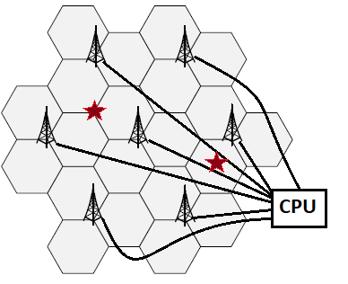
Figure 1: Dense Urban scenario according to [15] with BS sites coordinated through a CPU.

II-A Channel Model

The propagation and antenna models adopted follow the recommendations of the third generation partnership project (3GPP) Urban Macrocell model described in [15]. For simplicity, we assume that all UEs experience non-line-of-sight (NLOS) conditions. We will denote by $\beta_{mk}$ the large-scale gain between the $m$th TRP and the $k$th UE, which is conformed by the product of three components, $\beta_{mk}=\iota_{mk}\chi_{mk}\Gamma_{mk}$, detailed next. The path loss $\iota_{mk}$ between the $m$th TRP and the $k$th UE is chosen in accordance to [18], but has been modified to consider the presence of indoor UEs by adding a fixed wall penetration attenuation, i.e.,

$$\iota_{mk}=\left\{\begin{array}[]{cc}\iota_{0}+10\alpha\log_{10}(d_{mk})&\text{ outdoor UEs}\\ \iota_{0}+10\alpha\log_{10}(d_{mk})+\Delta_{\text{indoor}}&\text{ indoor UEs, }\\ \end{array}\right.$$ (1)

where $\iota_{0}$ is the path loss at the reference distance, $\alpha$ is the path loss exponent, $\Delta_{\text{indoor}}$ is the wall penetration loss, and $d_{mk}$ is the distance between the $m$th TRP and the $k$th UE. For completeness, we also define $P_{\text{ind}}$ as the probability for an arbitrary UE to be located indoors. The shadowing $\chi_{mk}$ is modeled as a correlated log-normal random variable with variance $\sigma_{\chi}^{2}$. The model describing its spatial correlation can be found in [7]. The radiating patterns of the antenna elements forming the antenna array installed at each TRP follow the specifications in [15, Table 9]. In the sequel, we will use $\vartheta_{mk}$ to denote the nominal angle-of-arrival (AoA) of the link between the $m$th TRP and the $k$th UE, seen from the TRP, and $\Gamma_{mk}$ to represent the directional gain of the antenna array in the direction of the $m$th TRP towards the $k$th UE.

It is assumed that the multi-path is characterized by spatially correlated Rayleigh fading, where the resulting channel matrix can be defined as $\boldsymbol{G}_{mk}=\left[\boldsymbol{g}_{mk1}\ldots\boldsymbol{g}_{mkN_{\text{UE}}^{k}}\right]\in\mathbb{C}^{N_{\text{TRP}}\times N_{\text{UE}}^{k}}$, with $\boldsymbol{g}_{mkn}$ denoting the channel vector from the $m$th TRP to the $n$th antenna on the $k$th UE (including both large-scale and small-scale fading). Spatial correlation matrices at both the transmit and receive antenna arrays are considered to conform to the popular Kronecker model, thus holding

$$\boldsymbol{G}_{mk}=(\boldsymbol{R}_{mk}^{\text{TRP}})^{1/2}\boldsymbol{G}_{mk}^{\text{iid}}(\boldsymbol{R}_{mk}^{\text{UE}})^{T/2},$$

with $\boldsymbol{G}_{mk}^{\text{iid}}$ representing an $N_{\text{TRP}}\times N_{\text{UE}}^{k}$ matrix of independent and identically distributed (iid) zero-mean circularly symmetric complex Gaussian random variables, and $\boldsymbol{R}_{mk}^{\text{UE}}$ and $\boldsymbol{R}_{mk}^{\text{TRP}}$ representing the spatial correlation matrices characterizing the scattering in the proximity of the UE and TRP antenna arrays, respectively. Following the model in [19, Chapter 2], $\boldsymbol{R}_{mk}^{\text{TRP}}$ and $\boldsymbol{R}_{mk}^{\text{UE}}$ can be calculated assuming an AoA that follows a Gaussian distribution around the nominal angles $\vartheta_{mk}^{\text{TRP}}$ and $\vartheta_{mk}^{\text{UE}}$, respectively. Defining $\boldsymbol{g}_{mk}=\text{vec}(\boldsymbol{G}_{mk})$, it is easy to check that

$$\boldsymbol{g}_{mk}\sim\mathcal{C}\mathcal{N}(\boldsymbol{0},\boldsymbol{R}_{mk}),$$

with $\boldsymbol{R}_{mk}=\boldsymbol{R}_{mk}^{\text{UE}}\otimes\boldsymbol{R}_{mk}^{\text{TRP}}$ and $\beta_{mk}=\frac{1}{N_{\text{TRP}}N_{\text{UE}}^{k}}\text{Tr}(\boldsymbol{R}_{mk})$.

Considering scenarios where UEs move slowly, it is reasonable to assume that the scattering covariance matrices $\boldsymbol{R}_{mk}^{\text{TRP}}$ and $\boldsymbol{R}_{mk}^{\text{UE}}$ change slowly, and can be perfectly known at the CPU and at the TRPs [7]. For later use, we define now the $MN_{\text{TRP}}\times N_{\text{UE}}$ composite channel between the $k$th UE and all the TRPs as $\boldsymbol{G}_{k}=\left[\boldsymbol{G}_{1k}^{T}\ldots\boldsymbol{G}_{Mk}^{T}\right]^{T}$, and its vectorized version as $\boldsymbol{g}_{k}=\text{vec}(\boldsymbol{G}_{k})$. The collective covariance matrix for the channel between the $k$th UE and all the TRPs can thus be defined as $\boldsymbol{R}_{k}=E\{\boldsymbol{g}_{k}\boldsymbol{g}_{k}^{H}\}=\mathcal{D}(\boldsymbol{R}_{1k},\ldots,\boldsymbol{R}_{Mk})$.

II-B Uplink training and channel estimation

In order to enable the estimation of the channel over each coherence time at the TRPs, each UE transmits a set of pilots, here referred to as pilot matrix $\boldsymbol{\Phi}_{k}$ of dimension $\tau_{p}\times N_{\text{UE}}^{k}$, that is, $\boldsymbol{\Phi}_{k}=[\boldsymbol{\varphi}_{k1}\ldots\boldsymbol{\varphi}_{kN_{\text{UE}}^{k}}]$, with $\boldsymbol{\varphi}_{kn}$ denoting the $\tau_{p}\times 1$ pilot sequence allocated to the $n$th antenna of the $k$th UE.

Interference among the antennas of UEs—or a given UE— during the channel estimation process is avoided by using a matrix of orthogonal pilot sequences, thus allowing the estimation of each individual channel $\boldsymbol{g}_{mkn}$. This implies that each pilot matrix $\boldsymbol{\Phi}_{k}$ fulfills $\boldsymbol{\Phi}_{k}^{H}\boldsymbol{\Phi}_{k}=\boldsymbol{I}_{N_{\text{UE}}^{k}}$. Whenever $N_{\text{str}}\leq\tau_{p}$, each UE can be allocated a pilot matrix orthogonal to the ones assigned to other UEs, i.e., $\boldsymbol{\Phi}_{k}^{H}\boldsymbol{\Phi}_{k^{\prime}}=\boldsymbol{0}_{N_{\text{UE}}^{k}\times N_{\text{UE}}^{k^{\prime}}}$ for any $k,k^{\prime}$. On the contrary, when $N_{\text{str}}>\tau_{p}$, some or all pilot matrices may need to be reused. In this work, the fingerprinting training introduced in [20] is applied, whereby pilot sequences are reused only by UEs which are located far apart from each other, aiming at reducing the pilot contamination effects. Note that a desirable side effect of guaranteeing the orthogonality among the pilot sequences transmitted from the different antennas of a UE is that channel estimation can be conducted independently for each antenna.

Denoting by $P^{\text{UE}}_{p}$ the available transit power per pilot at the UE, the received training samples at the $m$th TRP can be collected in an $N_{\text{TRP}}\times\tau_{p}$ matrix defined by

$${\boldsymbol{Y}_{p}}_{m}=\sum_{k=1}^{K}\sqrt{\tau_{p}P^{\text{UE}}_{p}/N_{\text{UE}}^{k}}\boldsymbol{G}_{mk}\boldsymbol{\Phi}_{k}^{T}+{\boldsymbol{N}_{p}}_{m},$$ (2)

where ${\boldsymbol{N}_{p}}_{m}\in\mathbb{C}^{N_{\text{TRP}}\times\tau_{p}}$ is a matrix of iid zero-mean circularly symmetric Gaussian random variables with standard deviation $\sigma_{u}$.

An estimate of $\boldsymbol{G}_{mk}$ that minimizes the minimum mean square error (MMSE) can be derived by first projecting the received pilot matrix ${\boldsymbol{Y}_{p}}_{m}$ onto the UE-specific pilot matrix [14]

$$\begin{split}\breve{\boldsymbol{Y}}_{p,mk}=&\left(\sum_{k^{\prime}=1}^{K}\sqrt{\tau_{p}P^{\text{UE}}_{p}/N_{\text{UE}}^{k^{\prime}}}\boldsymbol{G}_{mk^{\prime}}\boldsymbol{\Phi}_{k^{\prime}}^{T}\right)\boldsymbol{\Phi}_{k}^{*}\\ &+{\boldsymbol{N}_{p}}_{m}\boldsymbol{\Phi}_{k}^{*}.\end{split}$$ (3)

Using ${\boldsymbol{g}}_{mk}$ —the vectorized form of the channel matrix, linking the $k$th UE and the $m$th TRP—, it can be shown that the corresponding MMSE channel estimate follows [21, 7, 14]

$$\hat{\boldsymbol{g}}_{mk}=\sqrt{\frac{\tau_{p}P_{p}^{\text{UE}}}{N_{\text{UE}}^{k}}}\boldsymbol{R}_{mk}\boldsymbol{\Psi}_{mk}^{-1}\breve{\boldsymbol{y}}_{p,mk},$$ (4)

where $\breve{\boldsymbol{y}}_{p,mk}=\text{vec}(\breve{\boldsymbol{Y}}_{p,mk})$ and

$$\begin{split}\boldsymbol{\Psi}_{mk}=&\sum_{k^{\prime}=1}^{K}\frac{\tau_{p}P_{p}^{\text{UE}}}{N_{\text{UE}}^{k^{\prime}}}(\boldsymbol{\Phi}_{k}^{H}\boldsymbol{\Phi}_{k^{\prime}}\otimes\boldsymbol{I}_{N_{\text{TRP}}})\boldsymbol{R}_{mk^{\prime}}(\boldsymbol{\Phi}_{k^{\prime}}^{H}\boldsymbol{\Phi}_{k}\otimes\boldsymbol{I}_{N_{\text{TRP}}})\\ &+\sigma_{\upsilon}^{2}\boldsymbol{I}_{N_{\text{TRP}}N_{\text{UE}}^{k}}.\end{split}$$ (5)

Moreover, the distribution of the MMSE channel estimate can be shown to be

$$\hat{\boldsymbol{g}}_{mk}\sim\mathcal{C}\mathcal{N}\left(\boldsymbol{0},\frac{P_{p}^{\text{UE}}\tau_{p}}{N_{\text{UE}}^{k}}\boldsymbol{R}_{mk}\boldsymbol{\Psi}_{mk}^{-1}\boldsymbol{R}_{mk}\right),$$

whereas the distribution of the channel estimation error $\tilde{\boldsymbol{g}}_{mk}=\boldsymbol{g}_{mk}-\hat{\boldsymbol{g}}_{mk}$ conforms to $\tilde{\boldsymbol{g}}_{mk}\sim\mathcal{C}\mathcal{N}(\boldsymbol{0},\boldsymbol{A}_{mk})$, with

$$\boldsymbol{A}_{mk}=\boldsymbol{R}_{mk}-\frac{P_{p}^{\text{UE}}\tau_{p}}{N_{\text{UE}}^{k}}\boldsymbol{R}_{mk}\boldsymbol{\Psi}_{mk}^{-1}\boldsymbol{R}_{mk}.$$

Relying on the orthogonality of $\boldsymbol{\Phi}_{k}$, it is easy to check that the error covariance matrix possesses a block-diagonal structure, i.e.

$$\boldsymbol{A}_{mk}=\mathcal{D}(\boldsymbol{A}_{mk1},\ldots,\boldsymbol{A}_{mkN_{\text{UE}}^{k}}).$$

For convenience, we implicitly define $\hat{\boldsymbol{G}}_{mk}$, $\hat{\boldsymbol{G}}_{k}$ and $\hat{\boldsymbol{g}}_{k}$ as the MMSE-estimated counterparts of ${\boldsymbol{G}}_{mk}$, ${\boldsymbol{G}}_{k}$ and $\boldsymbol{g}_{k}$, respectively. It is worth pointing out at this stage that if a UE $k^{\prime}$ only activates $N_{\text{UE}}^{k^{\prime}}<N_{\text{UE}}$ antennas (i.e., it plans the reception of $N_{\text{UE}}^{k^{\prime}}$ data streams), its corresponding matrix pilot $\boldsymbol{\phi}_{k^{\prime}}$ only has dimensions $\tau_{p}\times N_{\text{UE}}^{k^{\prime}}$ with $\boldsymbol{\Phi}_{k^{\prime}}^{H}\boldsymbol{\Phi}_{k^{\prime}}=\boldsymbol{I}_{N_{\text{UE}}^{k^{\prime}}}$.

III Baseband processing

In this section, we introduce the baseband protocols used in this paper.

III-A UE association and TRP (de)activation

In the pursue of EE, we embrace that a number of TRPs can be shut down, and thus consider that only $M\leq M_{T}$ TRPs are active at any given instant. Following a UE-centric paradigm (see [8] for details), where each UE is served only by a subset of the active TRPs, we denote by $\boldsymbol{C}(\tau)$ the $M\times K$ connectivity matrix indicating which TRPs serve each UE over a specific large-scale propagation interval $\tau$. Its entries $c_{mk}(\tau)$ are configured as

$$c_{mk}(\tau)=\left\{\begin{array}[]{cc}1&\text{UE }k\text{ served by TRP }m\text{ over interval }\tau\\ 0&\text{otherwise.}\end{array}\right.$$ (6)

For convenience, and since results in the following subsections are derived for a single arbitrary large-scale interval, the index $\tau$ will be dropped from the connectivity matrix, i.e., $\boldsymbol{C}$ and $c_{mk}$ will be used instead of $\boldsymbol{C}(\tau)$ and $c_{mk}(\tau)$, respectively. We also define at this point the $1\times K$ vector $\boldsymbol{c}_{[m]}$ as the $m$th row of $\boldsymbol{C}$, which represents the connectivity of the $m$th TRP, and the $M\times 1$ vector $\boldsymbol{c}^{[k]}$ as the $k$th column of $\boldsymbol{C}$, which corresponds to the connectivity of the $k$th UE. We also denote sets $\mathcal{M}_{T}=\left\{m_{T}^{1},\cdots,m_{T}^{M_{T}}\right\}$ and $\mathcal{M}=\left\{m^{1},\cdots,m^{M}\right\}$ as the collections of all TRPs in the network and the active ones, respectively, holding $\mathcal{M}\subseteq\mathcal{M}_{T}$. Section V-B discusses our new method to devise the TRPs to shut down, filling in the entries of (6).

III-B Transmitter processing

The samples received by the $k$th UE can be expressed as

$$\boldsymbol{y}_{k}=\boldsymbol{G}_{k}^{T}\tilde{\boldsymbol{W}}\boldsymbol{s}+\boldsymbol{\upsilon}_{k},$$ (7)

where $\boldsymbol{s}=\left[\boldsymbol{s}_{1}^{T}\ldots s_{K}^{T}\right]^{T}$ is the $N_{\text{str}}\times 1$ vector of transmitted symbols, with $E\{\boldsymbol{s}^{H}\boldsymbol{s}\}=\boldsymbol{I}_{N_{\text{str}}}$ and $\boldsymbol{s}_{k}=[s_{k1}\ldots s_{kN_{\text{UE}}^{k}}]^{T}$, with $s_{kn}$ representing the information symbol for the $k$th UE on the $n$th stream, $\tilde{\boldsymbol{W}}$ is the $MN_{\text{TRP}}\times N_{\text{str}}$ precoding matrix (including transmit power allocation), and $\boldsymbol{\upsilon}_{k}\sim\mathcal{CN}(\boldsymbol{0},\sigma_{\upsilon}^{2}\boldsymbol{I}_{N_{\text{UE}}^{k}})$ is a vector of additive white Gaussian noise (AWGN) samples.

For convenience, we note that the global precoding matrix $\tilde{\boldsymbol{W}}$ can be defined on the basis of the TRP-specific blocks, that is, $\tilde{\boldsymbol{W}}=\left[\tilde{\boldsymbol{W}}^{1}\ldots\tilde{\boldsymbol{W}}^{M}\right]^{T}$, where $\tilde{\boldsymbol{W}}^{m}$ is the $N_{\text{TRP}}\times N_{\text{str}}$ precoding matrix applied at the $m$th TRP. It fulfils the transmit power constraint, $\|\tilde{\boldsymbol{W}}^{m}\|_{F}^{2}\leq P_{TRP}\ \forall m$. Alternatively, the precoder can be examined from a UE perspective by partitioning $\tilde{\boldsymbol{W}}$ as $\tilde{\boldsymbol{W}}=\left[\tilde{\boldsymbol{W}}_{1}\ldots\tilde{\boldsymbol{W}}_{K}\right]$, where $\tilde{\boldsymbol{W}}_{k}$ is the $MN_{\text{TRP}}\times N_{\text{UE}}^{k}$ block affecting the symbols $\boldsymbol{s}_{k}$ transmitted towards the $k$th UE. In turn, $\tilde{\boldsymbol{W}}_{k}$ can be decomposed into its constituent stream-oriented precoders as $\tilde{\boldsymbol{W}}_{k}=\left[\tilde{\boldsymbol{w}}_{k1}\ldots\tilde{\boldsymbol{w}}_{kN_{\text{UE}}^{k}}\right]$, allowing the received samples in (7) to be rewritten as

$$\begin{split}\boldsymbol{y}_{k}&=\boldsymbol{G}_{k}^{T}\sum_{k^{\prime}=1}^{K}\tilde{\boldsymbol{W}}_{k}\boldsymbol{s}_{k}+\boldsymbol{\upsilon}_{k}\\ &=\boldsymbol{G}_{k}^{T}\sum_{k^{\prime}=1}^{K}\sum_{n=1}^{N_{\text{UE}}^{k^{\prime}}}\tilde{\boldsymbol{w}}_{k^{\prime}n}s_{k^{\prime}n}+\boldsymbol{\upsilon}_{k}.\end{split}$$ (8)

In this paper, and without loss of generality, we use the centralized partial-MMSE (CP-MMSE) precoder design introduced in [22]. This precoder strives at a compromise between the strength of the desired signal transmitted at each UE and the interference it generates among the different UEs, wile preserving the scalability of the network. As a result, the $MN_{\text{TRP}}\times 1$ precoding vector targeting the $n$th stream of the $k$th UE can be expressed as

$$\tilde{\boldsymbol{w}}_{kn}=\sqrt{\frac{p^{\text{DL}}_{k}}{N_{\text{UE}}^{k}}}\frac{{\boldsymbol{w}}_{kn}}{\sqrt{E\{\|{\boldsymbol{w}}_{kn}\|^{2}\}}},$$ (9)

where the downlink transmit power $p_{k}^{\text{DL}}$ allocated to the $k$th UE is equally divided among its data streams, and

$$\boldsymbol{w}_{kn}=\frac{p_{k}^{\text{UL}}}{N_{\text{UE}}^{k}}\boldsymbol{\Omega}_{k}^{-1}\boldsymbol{C}^{[k]}\hat{\boldsymbol{g}}_{kn},$$ (10)

with

$$\begin{split}\boldsymbol{\Omega}_{k}&=\sum_{i\setminus\boldsymbol{c^{[k]}}^{T}\boldsymbol{c}^{[i]}>0}\frac{p_{i}^{\text{UL}}}{N_{\text{UE}}^{k}}\left(\boldsymbol{C}^{[k]}(\hat{\boldsymbol{G}}_{i}\hat{\boldsymbol{G}}_{i}^{H})\boldsymbol{C}^{[k]}+\boldsymbol{C}^{[k]}\boldsymbol{A}_{i}\boldsymbol{C}^{[k]}\right)\\ &+\sigma_{\upsilon}^{2}\boldsymbol{I}_{MN_{\text{TRP}}N_{\text{UE}}^{k}},\end{split}$$ (11)

where $\boldsymbol{C}^{[k]}=\mathcal{D}([\overbrace{\boldsymbol{c}^{[k],T}\ldots\boldsymbol{c}^{[k],T}}^{N_{\text{TRP}}N_{\text{UE}}^{k}}])^{T}$ and $\boldsymbol{A}_{i}=\mathcal{D}(\boldsymbol{A}_{1i}\cdots\boldsymbol{A}_{Mi})$. Note that the normalization step in (9) ensures that $E\{\|\tilde{\boldsymbol{w}}_{kn}\|^{2}\}=p_{k}^{\text{DL}}/N_{\text{UE}}^{k}$.

For the sake of preserving scalability principles, fractional power allocation is adopted [8], i.e.,

$$p_{k}^{\text{DL}}=\frac{P_{\text{TRP}}(\sum_{m=1}^{M}c_{mk}\beta_{mk})^{\upsilon}}{\max_{l\in\{1,\ldots,M\}}c_{lk}\sum_{i=1}^{K}c_{li}(\sum_{m=1}^{M}c_{mi}\beta_{mi})^{\upsilon}},$$ (12)

with $\upsilon\in[-1,1]$ denoting a parameter used to approximate the power allocation to different performance targets (e.g., sum-rate, max-min). Also note that the precoder depends on the uplink power allocation policy, which is set here in accordance to the uplink fractional power allocation described in [8, eq. (7.34)].

III-C Receiver processing

Having defined the processing done at the transmitter side, let us now consider the processing carried out at the UE. Towards this end, let us define ${\boldsymbol{\Xi}}_{kk^{\prime}}=\boldsymbol{G}_{k}^{T}\tilde{\boldsymbol{W}}_{k^{\prime}}$, thus leading to yet another reformulation of the received samples, i.e.,

$$\begin{split}\boldsymbol{y}_{k}&=\sum_{k^{\prime}=1}^{K}{\boldsymbol{\Xi}}_{kk^{\prime}}\boldsymbol{s}_{k^{\prime}}+\boldsymbol{\upsilon}_{k}\\ &=\underbrace{{\boldsymbol{\Xi}}_{kk}\boldsymbol{s}_{k}}_{\text{Useful signal}}+\underbrace{\sum_{k^{\prime}=1,k^{\prime}\neq k}^{K}{\boldsymbol{\Xi}}_{kk^{\prime}}\boldsymbol{s}_{k^{\prime}}}_{\text{Interference}}+\underbrace{\boldsymbol{\upsilon}_{k}}_{\text{Noise}}.\end{split}$$ (13)

Under the assumption of statistical channel state information (CSI) at the receiver (i.e., no pilots are transmitted on the downlink), only the mean of the equivalent channel affecting the useful term is available at the UE. Therefore it holds

$$\boldsymbol{y}_{k}=\bar{\boldsymbol{\Xi}}_{k}\boldsymbol{s}_{k}+\boldsymbol{e}_{k},$$ (14)

with $\bar{\boldsymbol{\Xi}}_{k}=E\{{\boldsymbol{\Xi}}_{kk}\}$ representing the average equivalent channel affecting the $k$th UE, and

$$\boldsymbol{e}_{k}=\sum_{k^{\prime}=1}^{K}{\boldsymbol{\Xi}}_{kk^{\prime}}\boldsymbol{s}_{k^{\prime}}-\bar{\boldsymbol{\Xi}}_{k}\boldsymbol{s}_{k}+\boldsymbol{\upsilon}_{k}$$ (15)

collecting the inter-UE interference, the self-interference (due to reliance on statistical CSI) and the AWGN noise.

Two different reception strategies are considered —namely, a linear one (MMSE) and a non-linear one (MMSE-successive interference cancellation (SIC))—, which are based on the availability of statistical CSI. These are now described in detail:

1. MMSE: A linear combiner is applied to the received samples to estimate the payload data symbols

   $$\hat{\boldsymbol{s}}_{k}=\boldsymbol{U}_{k}^{H}\boldsymbol{y}_{k}=\boldsymbol{U}_{k}^{H}\bar{\boldsymbol{\Xi}}_{k}\boldsymbol{s}_{k}+\boldsymbol{U}_{k}^{H}\boldsymbol{e}_{k},$$ (16)

   where re-expressing $\boldsymbol{U}_{k}=[\boldsymbol{u}_{k1}\ldots\boldsymbol{u}_{kN_{\text{UE}}^{k}}]$ and $\bar{\boldsymbol{\Xi}}_{k}=[\bar{\boldsymbol{\xi}}_{k1}\ldots\bar{\boldsymbol{\xi}}_{kN_{\text{UE}}^{k}}]$ allows the estimate of the $n$th symbol for the $k$th UE to be written as

   $$\hat{s}_{kn}=\boldsymbol{u}_{kn}^{H}\bar{\boldsymbol{\xi}}_{kn}s_{kn}+\boldsymbol{u}_{kn}^{H}\boldsymbol{b}_{kn},$$ (17)

   with $\boldsymbol{b}_{kn}=\sum_{n^{\prime}=1,n^{\prime}\neq n}^{N_{\text{UE}}^{k}}\bar{\boldsymbol{\xi}}_{kn^{\prime}}s_{kn^{\prime}}+\boldsymbol{e}_{k}$. An achievable downlink SE in bit/s/Hz for the $k$th UE can now be obtained as [8]

   $$R_{k}=\frac{1-\tau_{p}/\tau_{c}}{2}\sum_{n=1}^{N_{\text{UE}}^{k}}\log_{2}(1+\text{SINR}_{kn}),$$ (18)

   noting that the 1/2 factor is due to the assumption of an equal UL-DL split, and on the basis of (17), the instantaneous effective SINR for the $n$th stream of the $k$th UE follows

   $$\text{SINR}_{kn}=\frac{|\boldsymbol{u}_{kn}^{H}\bar{\boldsymbol{\xi}}_{kn}|^{2}}{\boldsymbol{u}_{kn}^{H}\boldsymbol{B}_{kn}\boldsymbol{u}_{kn}},$$ (19)

   where

   $$\boldsymbol{B}_{kn}=E\left\{\boldsymbol{b}_{kn}\boldsymbol{b}_{kn}^{H}\right\}=\sum_{n^{\prime}=1,n^{\prime}\neq n}^{N_{\text{UE}}^{k}}\bar{\boldsymbol{\xi}}_{kn^{\prime}}\bar{\boldsymbol{\xi}}_{kn^{\prime}}^{H}+\boldsymbol{E}_{k},$$ (20)

   with

   $$\begin{split}\boldsymbol{E}_{k}=E\left\{\boldsymbol{e}_{k}\boldsymbol{e}_{k}^{H}\right\}=&E\left\{\boldsymbol{G}_{k}^{T}\tilde{\boldsymbol{W}}\tilde{\boldsymbol{W}}^{H}\boldsymbol{G}_{k}^{*}\right\}\\ &-\bar{\boldsymbol{\Xi}}_{k}\bar{\boldsymbol{\Xi}}_{k}^{H}+\sigma_{\upsilon}^{2}\boldsymbol{I}_{N_{\text{UE}}^{k}}.\end{split}$$ (21)

   Since (19) has the form of a generalized Rayleigh quotient, this can be maximized by resorting to the MMSE combiner defined by [8]

   $$\boldsymbol{u}_{kn}=\boldsymbol{B}_{kn}^{-1}\bar{\boldsymbol{\xi}}_{kn},$$ (22)

   thus resulting in a maximum achievable SE

   $$R_{k}^{\text{MMSE}}=\frac{1-\frac{\tau_{p}}{\tau_{c}}}{2}\sum_{n=1}^{N_{\text{UE}}^{k}}\log_{2}(1+\bar{\boldsymbol{\xi}}_{kn}^{H}\boldsymbol{B}_{kn}^{-1}\bar{\boldsymbol{\xi}}_{kn}),$$ (23)

2. MMSE-SIC: SIC has been successfully adapted to the downlink of a cell-free network under the assumption of statistical CSI at the receiver [14] resulting in a SE

   $$R_{k}^{\text{MMSE-SIC}}=\frac{1-\frac{\tau_{p}}{\tau_{c}}}{2}\log_{2}\left|\boldsymbol{I}_{N_{\text{UE}}^{k}}+\bar{\boldsymbol{\Xi}}_{k}^{H}\boldsymbol{E}_{k}^{-1}\bar{\boldsymbol{\Xi}}_{k}\right|.$$ (24)

IV Power consumption model

To model the network power consumption, we use the realistic 4G/5G M-MIMO active antenna units (AAUs) model presented in [23]. In particular, and restricting to the case where each AAU operates a single carrier/cell, the power consumed by the AAU of the $m$th TRP when actively serving UEs is given by

$$\tilde{P}^{\text{AAU}}_{m}=\underbrace{P^{\text{AAU,fix}}+P^{\text{AAU,BB}}+P_{TRX}+P_{PA}}_{P_{Bline}}+\underbrace{\frac{1}{\eta}P^{TX}_{m}}_{P_{out}}$$ (25)

where $P^{\text{AAU,fix}}$ accounts for part of the AAU circuitry that is always active (e.g., circuitry used to control the AAU activation/deactivation), $P^{\text{AAU,BB}}$ is the power required for the baseband processing performed at the AAU, $P_{TRX}=\sum_{t=1}^{T}M_{av,t}D_{TRX,t}$ is the power consumed by the $T$ transceivers in the AAU (which can be calculated as the product of the number, $M_{av,t}$, of available RF chains and the power, $D_{TRX,t}$, consumed by each RF chain), $P_{PA}$ is the static power consumed by the power amplifiers (PAs), and $P_{out}$ is the power consumed by the transmit power (which is equal to the ratio of the transmit power, $P^{TX}_{m}=E\{\|\tilde{\boldsymbol{W}}^{m}\|_{F}^{2}\}$, to the efficiency of the PAs and antennas $\eta$). Note that the transmit power usually increases linearly with the number of resources utilized, and also depends on the specific baseband precoder implemented by each TRP. The first four terms are referred to as the baseline power consumption, denoted by $P_{Bline}$, and represent the overall power that an AAU requires to operate when there is no load.

As pointed out in [6], the ultra-lean signalling design, first proposed in 3GPP new radio (NR), paves the way for a more energy efficient operation of the TRPs. In particular, symbol shutdown mechanisms are enabled that can be operated over short timescales (i.e., from orthogonal frequency division multiplexing (OFDM) symbol level to 160 ms), and that can be combined with carrier shutdown and deep dormancy strategies, which progressively switch off more AAU hardware but can only react over coarser time scales (i.e., from seconds to minutes the former, and minutes and hours the latter).

Considering these shutdown methods, formally, the power consumption of the $m$th TRP can now be rewritten as

$$P^{\text{AAU}}_{m}=\left\{\begin{array}[]{cc}\tilde{P}^{\text{AAU}}_{m}&\text{ if }m\in\mathcal{M}\\ (1-\varpi)P_{Bline}&\text{ if }m\in\mathcal{M}_{T}\setminus\mathcal{M},\end{array}\right.$$ (26)

where $\varpi$ is the fraction of the baseline power saved when a TRP is in a shutdown mode. Recent studies have shown that, statistically, $\varpi$ takes average values of 0.3, 0.47 and 0.7 when using symbol shutdown, carrier shutdown and dormancy, respectively [23].

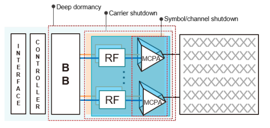
Figure 2: Power consumption model for AAU [23].

Aside from the AAU power consumption, and unlike classical cellular topologies, the CF-M-MIMO scheme must also consider the power consumption related to the extra infrastructure it requires, namely, the fronthaul links and the CPU. Following the results in [24], the power consumption of the fronthaul linking the $m$th TRP to the CPU over the downlink transmission phase can be expressed as

$$P_{m}^{\text{FH}}=\left\{\begin{array}[]{cc}P_{m}^{\text{FH,fix}}+\frac{\tau_{d}}{\tau_{c}}K_{\text{TRP}}P_{m}^{\text{FH,var}}&\text{ if }m\in\mathcal{M}\\ P_{m}^{\text{FH,fix}}&\text{ if }m\in\mathcal{M}_{T}\setminus\mathcal{M},\end{array}\right.$$ (27)

where $P_{m}^{\text{FH,fix}}$ and $P_{m}^{\text{FH,var}}$ are the fixed and rate-dependent power consumption of the $m$th fronthaul, respectively. The power consumption of the CPU can be modelled as [24]

$$P^{\text{CPU}}=P^{\text{CPU,fix}}+B\sum_{k=1}^{K}R_{k}P^{\text{CPU,pre}},$$ (28)

where $P^{\text{CPU,fix}}$ and $P^{\text{CPU,pre}}$ are the fixed and precoding-dependent power consumption of the CPU, respectively —the latter one being expressed in W/Gbps.

Having established the different terms, the total power consumption for the whole network when considering the full set $\mathcal{M}_{T}$ of TRPs is given by

$$P^{\text{TOT}}=\sum_{m=1}^{M_{T}}\left(P^{\text{AAU}}_{m}+P_{m}^{\text{FH}}\right)+P^{\text{CPU}}.$$ (29)

Relying on (18) and (29), we can now define the energy efficiency, $EE$, of the whole network over an arbitrary large-scale time interval as

$$EE=\frac{B\sum_{k=1}^{K}R_{k}}{P^{\text{TOT}}}[bits/J].$$ (30)

V Sleep mode and stream management

Having established the main processing steps and energy consumption requirements of a CF-M-MIMO network, and before delving into adaptive strategies, it is important to recap and clarify the time scales that apply to the different operations. In particular, three different time scales are considered here:

1. Short-scale: It is basically defined by the coherence time of the wireless channel. Pilot transmission (eq. (2)), channel estimation (eq. (4)) and precoder design (eq. (9)) are all processing steps that are conducted over a short-time scale. Power adaptation at this time scale is related to symbol shutdown mechanisms.

2. Large-scale: This is characterized by the changes experimented by large-scale propagation conditions (e.g., path loss, shadowing loss) and it is usually considered to span 40 to 100 channel coherence times. Pilot and power allocation (eq. (12)) are most often conducted on large-scale time basis as well as the combiner design at the receiver when relying only on statistical channel information. Power adaptation at this time scale is related to carrier shutdown mechanisms.

3. UE dynamics scale: This time scale is related to UE dynamics whose mobility patterns can span from minutes to hours or even days and weeks. It serves to define UE spatial probabilities that govern the UEs distribution across the coverage area. Power adaptation at this time scale is exploited using the TRP dormancy state.

In the coming subsections, we focus on adaptive mechanisms that are typically conducted at a large-scale (carrier shutdown), basically, because they exploit the large-scale propagation parameters (e.g., large-scale channel gains, correlation matrices). Particularly, in the two mechanisms covered next, UE stream management and TRP selective (de)activation, they are executed whenever significant changes in the large-scale propagation conditions take place with the decisions taken being effective over many coherence times. Nonetheless, some results are provided to hint what benefits bring the different power shutdown modes.

V-A Adaptive UE stream management

As described in Sec. II, it is assumed that all UEs are equipped with $N_{\text{UE}}$ antennas, thus allowing the reception of up to $N_{\text{UE}}$ data streams. However, as it will be shown next, it is not always advisable to allow the maximum degree of multiplexing to all UEs. The UEs adaptive stream management (ASM) described here refers to how to select the number of data streams ($N_{\text{UE}}^{k}$) per UE to optimize network performance. To this end, it is critical to recognize that allowing UEs to receive more than one data stream does not necessarily lead to enhanced performance due to two fundamental reasons:

1. Power split: All practical transmit power allocation strategies are rooted on large scale parameters (i.e., covariance matrices). Hence, the power devoted to a given UE on a per-coherence time basis (i.e., instantaneously) can only be uniformly split among the transmitted streams. This power division can cause that UEs experiencing bad propagation conditions have their SINR further degraded [14].

2. Increased pilot contamination: Antennas on any given UE must be assigned orthogonal pilots in order for their channels to be separated upon estimation, thus the constraint $\boldsymbol{\Phi}_{k}^{H}\boldsymbol{\Phi}_{k}=\boldsymbol{I}_{N_{\text{UE}}^{k}}$. Given a pilot length $\tau_{p}$, the pilot reuse factor, which in turn defines the number of interferers affecting the estimation of each channel, will be given by $\frac{\tau_{p}}{E\{N_{\text{str}}\}}$, which reduces to $\tau_{p}/K$ when all UEs just receive one single data stream and to $\tau_{p}/(KN_{\text{UE}})$ when all UEs aim at receiving as many data streams as antennas they have [25]. Logically, the more antennas the UEs activate, the larger the pilot contamination effect becomes.

Before delving into strategies on how to manage the UEs’ multiple antennas, it is worth assessing the performance of a CF-M-MIMO network when increasing the load for the specific case of single-antenna UEs. In particular, we focus on the total network rate (sum-rate) given by $R=\sum_{k=1}^{K}R_{k}$, where $R_{k}$ follows from (23), given a specific network configuration defined by the main setup parameters, $\boldsymbol{\Omega}=\{M,d_{\text{ISD}},N_{\text{TRP}},\tau_{p}\}$, where $d_{\text{ISD}}$ denotes the inter-site distance among neighbouring BSs. Figure 3 depicts the sum-rate when considering a network following the topology in Fig. 1, and when increasing the number of UEs per cell one UE per cell at a time (i.e., $K=21,42,63,\ldots$).

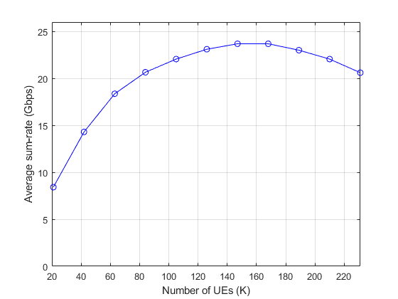
Figure 3: CF-M-MIMO sum-rate under different network configurations ($M=21$ TRPs, $\tau_{p}=30$ samples, $N_{\text{TRP}}=64$ antennas, $N_{\text{UE}}=1$ antenna).

It can be observed how the overall network sum-rate first increases as more UEs are admitted into the system, up to a point where it starts to decline, thus revealing that the pilot contamination effects outweigh the multi-UE diversity plus multiplexing gains. For the situation at hand, $\boldsymbol{\Omega}=\left\{21,200,64,30\right\}$, the optimum number of UEs seems to be approximately $K_{\boldsymbol{\Omega}}^{\text{opt}}\backsimeq 150$ (roughly 7 single-antenna UEs per hexagon in Fig. 1).

In the following, we propose a heuristic strategy to decide on the number of data streams per UE that, in alignment with the general cell-free philosophy, aims at protecting the worst-performing UEs in the network at the cost of sacrificing some of the potential improvements in rate for the UEs that are better off. Nonetheless, this strategy is generic enough to be adapted to other objectives.

The scheme starts by determining the maximum number of streams for a specific network layout $N_{\text{str}}$, and then fixing the groups of UEs with a prescribed number of streams, denoted as $\mathcal{K}^{(1)},\ldots,\mathcal{K}^{(N_{\text{UE}})}$, with $\mathcal{K}^{(i)}$ representing the set of UEs receiving $i$ data streams, whose cardinality is $K^{(i)}$. Note that $N_{\text{str}}\leq K_{\boldsymbol{\Omega}}^{\text{opt}}$ and that $\sum_{i=1}^{N_{\text{UE}}}K^{(i)}=K$. Towards this end, each UE $k$ is then assessed on the basis of two metrics:

1. Conditioning: $\xi_{k}=\lambda_{k}^{\text{max}}/\lambda_{k}^{\text{min}}$, with $\lambda_{k}^{\text{max}}$ and $\lambda_{k}^{\text{min}}$ denoting the maximum and minimum eigenvalues of ${\boldsymbol{R}}_{k}$. This metric measures the suitability of the corresponding channels to be favourably inverted by the MMSE filter design in (10).

2. Strength: ${\beta}_{k}=\text{Trace}({\boldsymbol{R}}_{k})$. This metric relates to the overall propagation gain a given UE is subject to.

For simplicity let us assume that UEs are split into two groups: Good UEs are those experiencing good conditioning and large strength, that is, those UEs with $\xi_{k}<\theta_{\xi}^{\text{good}}$ and ${\beta}_{k}>\theta_{\beta}^{\text{good}}$, with $\theta_{\xi}^{\text{good}}$ and $\theta_{\beta}^{\text{good}}$ representing adequate thresholds that must be determined by simulation. In the numerical results section, specific numerology is given, but it has been found that overall network performance is not overly sensitive to these values. These UEs are the ones that can safely support multi-stream transmission, and thus potentially conform sets $\mathcal{K}^{(2)},\ldots,\mathcal{K}^{(N_{\text{UE}})}$. In contrast, bad UEs are those subject to bad conditioning and large propagation losses, and thus must be limited to single-stream transmissions, and assigned to $\mathcal{K}^{(1)}$. In general setups, UEs will need to be classified into $N_{\text{UE}}$ groups, thus the quantitative evaluation of goodness should be done by fixing $N_{\text{UE}}-1$ thresholds on both metrics ($\theta_{\xi}^{\text{good},1},\ldots,\theta_{\xi}^{\text{good},N_{\text{UE}}-1},\theta_{\beta}^{\text{good},1},\ldots,\theta_{\beta}^{\text{good},N_{\text{UE}}-1}$). To this end, the following recursive strategy is proposed here: We start by aiming at a first split of UEs into two groups, $\mathcal{K}^{(1)}$ and $\mathcal{K}_{\text{rest}}^{(1)}$, formed by those UEs that are assigned one and more than one data streams, respectively. The objective now is to guarantee that UEs in $\mathcal{K}^{(1)}$ achieve virtually the same performance as if $\mathcal{K}^{(1)}=\mathcal{K}$ (all UEs were assigned one data stream). As a result, the set of all available pilot sequences, $\mathcal{P}$, is split into two groups $\mathcal{P}_{1}$ and $\mathcal{P}_{\text{rest}}^{(1)}$, where it should be guaranteed that

$$\frac{K^{(1)}}{|\mathcal{P}_{1}|}=\frac{K}{\tau_{p}},$$

hence

$$|\mathcal{P}_{1}|=\text{round}\left\{\frac{K^{(1)}\tau_{p}}{K}\right\}\ \text{and}\ |\mathcal{P}_{\text{rest}}^{(1)}|=\tau_{p}-|\mathcal{P}_{1}|.$$ (31)

The split of pilots according to (31) aims at guaranteeing that the worst UEs are not affected by the increased pilot contamination due to multi-stream transmission. In fact, note that (31) ensures that that UEs in $\mathcal{K}^{(1)}$ have available (approximately), the same number of pilots they had in the initial setup when all UEs had only one stream assigned. This procedure is generalized to as many groups as potential number of data streams by successively applying the same technique on the UE and pilot sets, $\mathcal{K}_{\text{rest}}^{(1)}$ and $\mathcal{P}_{\text{rest}}$, respectively, that is, splitting $\mathcal{K}_{\text{rest}}^{(1)}$ into $\mathcal{K}^{(2)}$ and $\mathcal{K}_{\text{rest}}^{(2)}$, and $\mathcal{P}_{\text{rest}}^{(1)}$ into $\mathcal{P}_{2}$ and $\mathcal{P}_{\text{rest}}^{(2)}$. The general procedure to generate the UE and pilot groups is detailed in Algorithm 1. As shown in the algorithmic description, and after suitably initializing all variables in use, the aim is to create up to a maximum of $N_{\text{UE}}$ groups of UEs each characterized by the number of streams each group is able to handle (from $1$ up to $N_{\text{UE}}$). Towards this end, it first tries to determine whether there are UEs with good enough propagation conditions (as determined by $\theta_{\xi}^{\text{good,g}}$ and $\theta_{\beta}^{\text{good,g}}$) and subsequently evaluates whether there are enough pilot symbols to guarantee the contention of pilot contamination effects affecting the UEs with worst channels. When both conditions are fulfilled, a new group $\mathcal{K}^{(g)}$ is born with a prescribed group-specific pilot allocation $\mathcal{P}_{g}$. If at any point in the loop the number of allocated streams $L$ exceeds $N_{\text{str}}$, the algorithm stops leaving other groups are left empty.

Algorithm 1 UE stream selection based on large-scale propagation parameters.

Necessary condition: $K<N_{\text{str}}$

Inputs: $\mathcal{K}$, $\mathcal{P}$, $N_{\text{UE}}$, $N_{\text{str}}$, $\beta_{mk},\boldsymbol{R}_{k}\ \ \forall m,k$,

$\theta_{\xi}^{\text{good},1},\ldots,\theta_{\xi}^{\text{good},N_{\text{UE}}-1},\theta_{\beta}^{\text{good},1},\ldots,\theta_{\beta}^{\text{good},N_{\text{UE}}-1}$.

$\forall k$ Compute strength and UE conditioning:

$$\beta_{k}=\text{Trace}(\boldsymbol{R}_{k})\text{ and }\xi_{k}=\lambda_{k}^{\text{max}}/\lambda_{k}^{\text{min}}\text{, where }$$

$$\lambda_{k}^{\text{max}}=\max\{\text{eigs}(\boldsymbol{R}_{k})\},\lambda_{k}^{\text{min}}=\min\{\text{eigs}(\boldsymbol{R}_{k})\},$$

$L=K$ (Total umber of streams allocated. At least 1 per UE).

$\mathcal{K}^{(1)}=\ldots=\mathcal{K}^{(N_{\text{UE}})}=\emptyset$

$\mathcal{K}^{(0)}_{\text{rest}}=\mathcal{K}$

$\mathcal{P}_{1}=\ldots=\mathcal{P}_{N_{\text{UE}}}=\emptyset$

$\mathcal{P}^{(0)}_{\text{rest}}=\mathcal{P}$

$g=1$

while $(g<N_{\text{UE}})$ and $(L<N_{\text{str}})$ do
        $\hat{\mathcal{K}}=\left\{k\in\mathcal{K}^{(g-1)}_{\text{rest}}:\beta_{k}>\theta_{\beta}^{\text{good},g}\text{ and }\xi_{k}<\theta_{\xi}^{\text{good},g}\right\}$

if $|\hat{\mathcal{K}}|<(N_{\text{str}}-L)$ then
                $\mathcal{K}^{(g)}_{\text{rest}}=\hat{\mathcal{K}}$

$\mathcal{K}^{(g)}=\mathcal{K}^{(g-1)}_{\text{rest}}-\hat{\mathcal{K}}$

else
                $\hat{\mathcal{K}}_{\text{tmp}}=\{k\in\hat{\mathcal{K}}\text{ with }(N_{\text{str}}-L)-|\hat{\mathcal{K}}|\text{ largest }\beta_{k}\}$

$\mathcal{K}^{(g)}_{\text{rest}}=\hat{\mathcal{K}}_{\text{tmp}}$

$\mathcal{K}^{(g)}=\mathcal{K}^{(g-1)}_{\text{rest}}-\hat{\mathcal{K}}_{\text{tmp}}$

end
        $L=L+|K^{(g)}_{\text{rest}}|$

$|\mathcal{P}_{g}|=\text{round}\left\{\frac{|\mathcal{K}^{(g)}||\mathcal{P}_{g-1}|}{|\mathcal{K}^{(g-1)}|}\right\}$

$\mathcal{P}_{g}=\{|\mathcal{P}_{g}|\text{ columns of }\mathcal{P}_{\text{rest}}^{(g-1)}\}$

if $\mathcal{P}_{g}=\emptyset$ (Not enough pilot symbols)

$\mathcal{K}^{(g)}=\emptyset$

$\mathcal{K}^{(g)}_{\text{rest}}=\emptyset$

break from while loop

end

$g=g+1$

end
Output: UE groups $\mathcal{K}^{(1)},\ldots,\mathcal{K}^{(N_{\text{UE}})}$

Pilot groups $\mathcal{P}_{1},\ldots,\mathcal{P}_{N_{\text{UE}}}$.

V-B Adaptive TRP (de)activation

The adaptive TRP (de)activation proposed in this paper targets the maximization of the overall network EE subject to a constraint on the achieved SE. Given the baseband processing introduced in Section III, the only degree of freedom left to tune the network performance is the setting of the connectivity matrix $\boldsymbol{C}$, which is initially subject to constraints, if scalability needs to be guaranteed. Formally, fixing a prescribed number of active TRPs, the design of $\boldsymbol{C}$ is governed by the following optimization problem

$$\begin{split}&\operatorname*{arg\,max}_{\boldsymbol{C}}{EE}\\ \quad&\text{ subject to}\\ \quad&\quad\quad\quad\|\boldsymbol{c}_{[m]}\|_{1}\leq K_{\text{TRP}}\ \ \ \forall m\in\mathcal{M}\\ \quad&\quad\quad\quad\|\boldsymbol{c}^{[k]}\|_{1}\geq 1\ \ \ \forall k\\ \quad&\quad\quad\quad f(\{R_{k}\})\geq R_{0}\ \ \ \forall k,\\ \end{split}$$ (32)

where the first restriction ensures the scalability of the network, the second ensures that no UE is left without connection, and the third establishes a general rate restriction, with $f(\cdot)$ denoting an arbitrary function of the achievable SE experienced by all UEs. Popular choices for this function could be the average, the minimum or a certain percentile of the UEs’ rates. Note that this optimization problem implicitly involves determining how many TRPs are active ($M$), and which ones. Some remarks are in place:

1. The minimum rate constraint unavoidably implies that problem (32) may not be feasible, in which case, an outage occurs.

2. Any TRP $m$, for which $\|\boldsymbol{c}_{[m]}\|_{1}=0$, belongs to $\mathcal{M}_{T}\setminus\mathcal{M}$, and thus the TRP power consumption is reduced in accordance to (26).

3. The CF-M-MIMO scheme can be turned into a conventional co-located (cellular) M-MIMO by activating all TRPs, i.e. $\mathcal{M}=\mathcal{M}_{T}$, and setting the $K$ columns of $\boldsymbol{C}$ as

   $$\boldsymbol{c}^{[k]}=[\underbrace{0\ldots 0}_{m_{k}-1}\ 1\ \underbrace{0\ldots 0}_{M-m_{k}+1}]^{T},$$ (33)

   where $m_{k}=\operatorname*{arg\,max}_{m}\beta_{mk}$, in which case every TRP solely serves the UEs within its cell (here it is assumed that UE-association is conducted on the basis of minimum propagation losses, or equivalently, maximum received signal strength).

4. We note the absence of a per-TRP maximum power constraint in problem (32). The reason is that by adhering to the fractional power allocation in (12), such restriction is guaranteed to be fulfilled.

Problem (32) is a constrained binary optimization problem, whose solution requires an exhaustive search over all candidate $\boldsymbol{C}$ matrices. Since this approach quickly becomes computationally impractical, even for moderate values of $M_{T},M$ or $K$, alternative solutions need to be sought.

We first propose an heuristic to approach the solution of (32) that relies on the dynamic cluster formation (DCF) from [8], while ensuring:

1. $\mathcal{M}=\mathcal{M}_{T}$.

2. Each TRP $m\in\mathcal{M}$ serves the $K_{TRP}$ UEs experiencing the largest large-scale gains. That is, the connectivity vector of the $m$th TRP $\boldsymbol{c}_{\text{[m]}}$ is defined as

   $$\boldsymbol{c}_{mk}=\left\{\begin{array}[]{cc}1&\text{ if }\beta_{mk}\in\mathcal{S}_{m}^{K_{TRP}}\\ 0&\text{ otherwise }\end{array}\right.,$$ (34)

   where $S_{m}^{K_{TRP}}$ is the set formed by the largest $K_{TRP}$ entries of all large-scale gains involving the $m$th TRP.

3. For any UE $k^{\prime}$, for which $\|\boldsymbol{c}^{[k^{\prime}]}\|_{1}=0$ (orphan UE), its strongest TRP is identified by $m_{k^{\prime}}=\operatorname*{arg\,max}_{m}\beta_{mk^{\prime}}$, and the connectivity of TRP $m_{k^{\prime}}$ is modified by setting:

   $$c_{m_{k^{\prime}}k^{\prime}}=1\text{ and }c_{m_{k^{\prime}}i}=0,$$ (35)

   where $i=\operatorname*{arg\,min}_{i}S_{m_{k^{\prime}}}^{K_{TRP}}$. This step trades the weakest UE selected by TRP $m_{k^{\prime}}$ by the orphan UE.

This heuristic proceeds in a greedy fashion switching off at each step the TRP that maximizes the EE, while satisfying the constraints in (32). This method, however, is still computationally intensive as it involves repeatedly calculating (10).

Striving for a simpler solution to Problem (32), we introduce here a lower-complexity greedy alternative that determines the TRP to be switched off by only relying on the large-scale propagation losses rather than on the achievable rates. The algorithm proposed builds on previous proposals [10, 26], but noting that, unlike in classical (non-regular) CF-M-MIMO deployments, here $K\gg{M}$. The algorithm proceeds in a greedy fashion aiming at switching off at each step (indexed by $l$) the TRP whose large-scale losses has the least performance degradation for the overall UE population.

In order to formalize this strategy, summarized in Alg. 2, let us define set $\boldsymbol{\beta}_{\mathcal{K}}=[\boldsymbol{\beta}_{1}\ldots\boldsymbol{\beta}_{K}]$ with $\boldsymbol{\beta}_{k}=[\beta_{1k}\ldots\beta_{Mk}]$ representing the vector containing all the large-scale propagation gains from the $k$th UE to all active TRPs. At each step $l$ of the algorithm, the goal is to reduce the set of active TRPs from $\mathcal{M}^{(l-1)}$ to $\mathcal{M}^{(l)}$ by removing the TRP $m^{\prime}$ that has less performance impact on the UEs. Further refining the notation, when beginning step $l$ of the algorithm, the UE-specific signature vector is defined by $\boldsymbol{\beta}_{k}^{(l)}=[\beta_{1k}\ldots\beta_{M^{(l-1)}k}]$, which comprises the gains to the set of active TRPs $\mathcal{M}^{(l-1)}$. In order to identify the TRP $m^{\prime}$ to switch off, UEs are clusterized into $M^{(l)}-1$ disjoint sets on the basis of their signature-vector $\boldsymbol{\beta}_{k}^{(l)}$. Popular clustering techniques, such as $k$-means, can be used to partition at each step the set of all UE into clusters $\mathcal{K}^{(l)}$, i.e., $\mathcal{K}^{(l)}=\{\mathcal{K}_{1},\ldots,\mathcal{K}_{M^{(l)}}\}$. This clustering step will naturally tend to group together those UEs that lie geographically close [27]. Aside from a cluster index, $k$-means also returns the centroid of each cluster $c$, i.e., $\bar{\boldsymbol{\beta}}_{\mathcal{K}^{(l)}}(c)$, with $c\in(1,M^{(l)})$.

At the $l$th step, the algorithm proceeds to first select (in an ordered manner) the TRPs exhibiting the minimum propagation losses to each of the $M^{(l)}$ centroids. In a second step, after removing the already selected TRPs from the set of selectable ones, the procedure is repeated. That is, the algorithm again orderly selects the TRPs, out of the remaining ones, whose propagation losses to each of the $M^{(l)}$ centroids is minimum. This procedure is repeated until the number of selected TRPs is equal to $M^{(l)}=M^{(l-1)}-1$ . Finally, the EE of the network with such configuration is estimated using (30). This procedure is repeated until the maximum EE is identified, while satisfying the constraints in (32), or there are no more TRPs to be turned off.

Algorithm 2 Greedy-efficient adaptive algorithm based on large-scale propagation losses.

Inputs: $R_{0},\mathcal{M}_{T},K_{\text{TRP}},\beta_{mk}\ \ \forall m,k\in\mathcal{M}_{T}$.

Initialization: Apply DCF calculating $\mathcal{M}=\mathcal{M}_{T}$ and setting $\boldsymbol{c}_{\text{[m]}}$ for all $m$ using (34) and (35).

Estimate UEs’ rates $R_{k}\ \ \forall k$, using (18).

Estimate baseline energy efficiency, EE⁽⁰⁾, using (30).

$\mathcal{M}^{(0)}=\mathcal{M}_{T}$, $M^{(0)}=M_{T}$, $\boldsymbol{\beta}_{\mathcal{K}}^{(0)}=\boldsymbol{\beta}_{\mathcal{K}}$. $l=1$. $m^{\prime}=\emptyset$

While ($f(\{R_{k}\})\geq R_{0}$) and ($l<M$)

if $K>M^{(l-1)}$ then
              $M^{(l)}=M^{(l-1)}-1$,

Use k-means to construct $M^{(l-1)}$ UE clusters

$\mathcal{K}^{(l)}=\{\mathcal{K}_{1},\ldots,\mathcal{K}_{M^{(l-1)}}\}$ with centroids

$\bar{\boldsymbol{\beta}}_{\mathcal{K}^{(l)}}=\{\bar{\boldsymbol{\beta}}_{\mathcal{K}_{1}},\ldots,\bar{\boldsymbol{\beta}}_{\mathcal{K}_{M^{(l-1)}}}\}$.

$\mathcal{J}$=Orderly collect from set $\bar{\boldsymbol{\beta}}_{\mathcal{K}^{(l)}}$ the $\mathcal{M}^{(l)}$ TRPs

with largest virtual propagation gains.

$m^{\prime}=\mathcal{M}^{(l-1)}\setminus\mathcal{J}$

else
              $\mathcal{J}$=Orderly collect from set ${\boldsymbol{\beta}}_{\mathcal{K}^{(0)}}$ the $\mathcal{M}^{(l)}$ TRPs

with largest large-scale gains.

$m^{\prime}=\mathcal{M}^{(l-1)}\setminus\mathcal{J}$

end if

Update energy efficiency, EE^(l).

if (EE${}^{(l)}<$EE^(l-1)) then
              Break from while loop

else
             $l=l+1$.

Update connectivity matrix $\mathbf{C}$ by removing the $m^{\prime}$th row.

Update active TRPs: $\mathcal{M}^{(l)}=\mathcal{M}^{(l-1)}\setminus m^{\prime}$.

end if
end while .

Output: Connectivity matrix $\mathbf{C}$.

VI Numerical results

As discussed in Section II, the scenario considered is inspired by the eMBB dense urban scenario test environment in [15], depicted in Fig. 1, where in this case, $L=7$, $S=3$ and thus $M_{T}=21$. The inter-site distance is set to 200 m. Wrap-around is applied to the target coverage area to eliminate boundary effects from the simulation results. Every TRP is equipped with a full digital array of $N_{TRP}=64$ antenna elements, configured as an $16\times 4$ uniform rectangular array (URA), with each antenna element connected to a transceiver chain. The third constraint in Problem (32) has been imposed on the average rate as per the IMT-2020 requirements, i.e., the EE maximization should fulfill $E\{R_{1},\ldots,R_{K}\}\geq R_{0}$ with $R_{0}=100$ Mbps. Table I presents the rest of parameters used.

TABLE I: Summary of default simulation parameters

Parameter (symbol)	Value
Carrier frequency ($f_{c}$):	2 GHz
Bandwidth ($B$)	100 MHz
Fixed TRP power ($P_{fix}$)	500 W
Maximum radiated TRP power ($P_{out}$)	240 W
CPU power consumption ($P^{\text{CPU,fix}},P^{\text{CPU,pre}}$)	5 W, 0.1 W/Gbps
Fronhtaul power consumption ($P_{m}^{\text{FH,fix}},P_{m}^{\text{FH,var}}$)	0.825 W, 0.01 W
Fractional power allocation factor ($\upsilon$)	-0.5
TRP $/$ UE antenna height ($h_{TRP}/h_{UE}$)	25 m $/$ 1.65 m
Coherence interval length ($\tau_{c}$)	200 samples
Training phase length ($\tau_{p}$)	20 samples
Pathloss parameters ($\iota_{0}$, $\alpha$, $\sigma_{\chi}$)	30, 3.67, 4
Shadow fading decorrelation distance ($d_{\text{dcorr}}$)	9 m
Shadow fading correlation among TRPs	0.5
Distribution of the AoA deviation	$\zeta\sim\mathcal{N}(0,\sigma_{\zeta}^{2})$
Azimuth Angular standard deviations ($\sigma_{\zeta}^{A}$)	$15^{\circ}$
Elevation Angular standard deviations ($\sigma_{\zeta}^{E}$)	$10^{\circ}$

VI-A Benefits of cell-free processing

The first question that must be answered is whether cell-free processing offers a significant throughput advantage over classical cellular-based M-MIMO processing when applied over a regular topology. Towards this end, Fig. 4 depicts the cumulative distribution functions (CDFs) of the UE’s rates when $K=84$ UEs. Two distinct situations are considered: One where all UEs are outdoors ($P_{ind}=0.0$) and another one where half of the UEs are indoors ($P_{ind}=0.5$). In both cases, we follow the guidelines in [15] that presume that UEs are evenly distributed among the 21 hexagonal cells, and uniformly distributed within each cell. For the case of all-outdoor UEs, results show how CF-M-MIMO processing offers a considerable advantage. For the 10%-tile of worst UEs, the CF-M-MIMO reaches 175 Mbps, whereas the cellular M-MIMO network falls below 70 Mbps, a 2.5$\times$ increase. When considering that some of the UEs are indoors, CF-M-MIMO keeps offering a substantial advantage for the best performing UEs. However, this benefit reduces. When considering the 10%-tile of worst UEs, which invariably corresponds to indoor UEs suffering the extra 20 dB loss due to wall propagation, CF-M-MIMO still offers a 1.6$\times$ gain w.r.t. cellular M-MIMO (from 15 Mbps to 9 Mbps). The change in the silhouette of the CF-M-MIMO curve when $P_{ind}=0.5$ is due to its different ability to serve indoors and outdoors UEs.

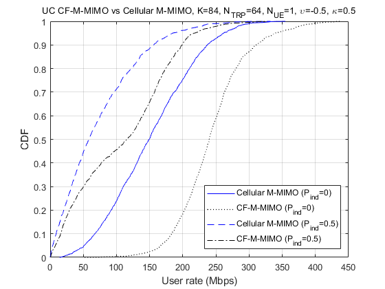
Figure 4: CF-M-MIMO vs Cellular UE rate CDF comparison when $K=84$ single-antenna UEs ($N_{UE}=1$).

Turning now our attention to the case of a more heavily loaded network, shown in Fig. 5 (8 UEs per hexagon), it is clear that the sharing of the TRPs available transmit power among more UEs together with the larger amount of interference causes the per-UE rates to drastically fall. In fact, note that $K=168$ UEs is beyond the optimum load point, as shown in Fig. 3. Nonetheless, most of the insights drawn when $K=84$ UEs still hold with the CF-M-MIMO approach doubling the rate achieved by the worse 10$\%$ of UEs in the fully-outdoor scenario. Unfortunately, note how both cellular and CF-M-MIMO architectures have difficulties in handling indoor UEs, as evidenced by the dashed lines in Fig. 5, thus reinforcing the importance of properly dimensioning the network to the traffic needs.

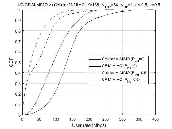
Figure 5: CF-M-MIMO vs Cellular UE rate CDF comparison when $K=168$ single-antenna UEs ($N_{UE}=1$).

VI-B Benefits of adaptive UE stream management

As mentioned in the introduction, most CF-M-MIMO literature focuses on single-antenna UEs, thus obviating the fact that currently deployed fifth generation (5G) networks must deal with UEs equipped with a larger number of antennas. In order to assess this condition, Fig. 6 shows the rate performance of a CF-M-MIMO network with $K=42$ UEs equipped with either 1, 2 or 4 antennas, and receiving as many data streams as receive antennas. This figure depicts the rate CDF attained when UEs rely on either of the detection schemes introduced in Section III (i.e., MMSE or MMSE-SIC). First point to notice is that increasing the number of received streams per UE favours the use of the more advanced MMSE-SIC detector over MMSE. In particular, there is no difference between the two detectors for $N_{\text{UE}}=1$, a very marginal improvement for $N_{\text{UE}}=2$ and a clear gain for $N_{\text{UE}}=4$. An even more remarkable observation is the relative performance attained for the different values of $N_{\text{UE}}$. Whereas the configuration for $N_{\text{UE}}=2$ clearly outperforms single-antenna setups ($N_{\text{UE}}=1$), increasing to $N_{\text{UE}}=4$ is a rather compromising option: For the worst UEs, actually allowing them to receive 4 streams ($N_{\text{UE}}=4$) degrades their rate performance below the one that can be achieved when only one stream is received. Furthermore, only a very limited number of UEs (those with extremely favourable channel conditions) are able to actually gain some rate over that achieved when only activating the reception of two data streams. Note that, in this case, $N_{\text{str}}=KN_{\text{UE}}=42\times 4=168$, which significantly exceeds the predicted maximum multiplexing gain $K_{\boldsymbol{\Omega}}^{\text{opt}}=150$, hence explaining the degraded performance observed for $N_{\text{UE}}=4$. These results illustrate the need to apply the ASM scheme introduced in Section V-A.

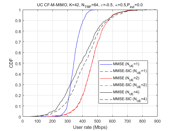
Figure 6: CDF of UE rate for CF-M-MIMO when $K=42$ UEs and varying number of the UE antennas.

To this end, we now consider the case of an scenario with $K=84$ active UEs with multi-antenna capabilities defined by $N_{\text{UE}}=2$. Since each UE can process up to two streams, the ASM mechanism introduced in Section V.A must configure thresholds $\theta_{\xi}^{\text{good,1}}$ and $\theta_{\beta}^{\text{good,1}}$, which in the results shown next have been fixed to $\theta_{\beta}^{\text{good,1}}=0.5$ and $\theta_{\xi}^{\text{good,1}}=0.9$. These values provide a good balance, combining an increase in the multiplexing capabilities of the best UEs, while preserving the rates of the weakest UEs. We note that these parameters are not overly sensitive and work well on a relatively wide range on numbers.

Figure 7 compares the SINR performance when having one or two antennas at the UEs for both, cellular and cell-free topologies. All results assume the use of the MMSE-SIC detector. Also note that SINR depicted for the two-antenna case actually corresponds to the average SINR experienced by the UEs on both receive antennas. From the figure, it can be seen that activating the reception of multiple streams (i.e., using two antennas at the UE) always results in an SINR degradation mainly due the split of the available transmit power that impinges each data stream. Moreover, Figure 7 also shows how CF-M-MIMO attains larger SINR values than the corresponding cellular deployments —a fact that could already be foreseen from the rate results shown in Fig.4. Importantly, these results also indicate the better SINR performance when using the ASM scheme introduced in Section V-A.

Clearly, the adaptive scheme improves the SINR performance over the two-stream counterpart. In particular, this improvement is especially clear in the lower SINR range.

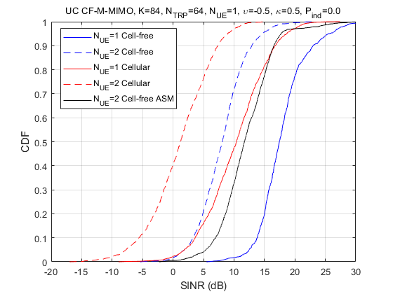
Figure 7: CDF of per-stream SINR for CF-M-MIMO and Cellular when $K=84$ UEs.

Despite the hint provided by the SINR results, it is upon the examination of the rate results in Fig. 8 that most insights can be gathered. Noticeably, for both cellular and CF-M-MIMO, it can be observed how, for the lowest rate region, the single-stream configuration substantially improves the rate results obtained when using two-stream UEs. As forecasted in Section V-A, the increase in pilot sequence re-use (that in turns increases pilot contamination) together the power split cause the two-stream configurations to be severely harmed for the UEs that are worse-off. In contrast, it can be seen that in the highest rate range, characterized by those UEs experiencing a strong channel gain and good conditioning, the two-stream configuration is superior to the single-stream counterpart. It is in this figure where the benefits of the ASM technique become most apparent. In this specific case, the maximum number of data streams has been conservatively set to $N_{\text{str}}=135(<K_{\boldsymbol{\Omega}}^{\text{opt}})$. Note in Fig. 8 how for the lowest rate range, the ASM mechanisms basically assigns a single data stream to those UEs that are worse off, while it assigns two data streams to those UEs that are experiencing good propagation conditions. In particular, the 10% of the worst UEs only suffer from a degradation of around 3-4% with respect to that achieved when using a single data stream (from 197 to 188 Mbps), rather than the 15% degradation experienced when all UEs are allowed to use two data streams (from 197 Mbps to 163 Mbps). Complementing these results, note how that for the best UEs, the ASM approach manages to reap off most of the benefits brought by multiple receive antennas at the UE side by allowing those UEs to receive two data streams.

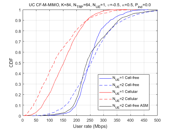
Figure 8: CDF of UE rate for CF-M-MIMO and Cellular when $K=84$ UEs for different number of antennas/streams.

VI-C Benefits of adaptive TRP (de)activation

Having established the benefits CF-M-MIMO processing can bring to a regular topology, we address now the maximization of the network glsEE through the application of the selective TRP activation algorithm introduced in Section V-B. To fully appreciate the benefits of the greedy TRP switch-off, we assume the presence of two hotspots in the coverage area serving $K=84$ UEs. In particular, and fixing the central tower in Figure 1 to be situated at $(0,0)$ m, the two hostspots centres are (arbitrarily) located at $(-100,57.75)$ m and $(200,-57.75)$ m (solid stars in Fig. 1), and following the guidelines in [28], 2/3 of the UEs are thrown at either one of the two hotspot areas (within a 40 m radius of the hotspot central location), while the remaining third is uniformly deployed throughout the coverage area. In terms of energy consumption, we consider the most conservative fixed-power reduction factor, $\xi=0.3$, corresponding to symbol shutdown operation [23], presaging that more aggressive sleep modes will result in even larger energy savings. In order to benchmark the effectiveness of the proposed approach, and as done in the literature, the reference used is the random switch-off of TRPs [10].

Figures 9 and 10 respectively depict the average EE and SE achieved by the cellular M-MIMO and CF-M-MIMO setups when executing either random or greedy switch-off. The most apparent observation is the clear superiority that the CF-M-MIMO exhibits over cellular in terms of both EE and SE.

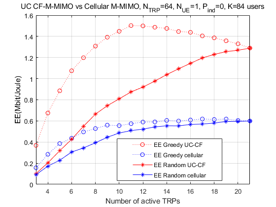
Figure 9: CF-M-MIMO vs Cellular adaptive switch-off EE performance when $K=84$ UEs with hotspots.

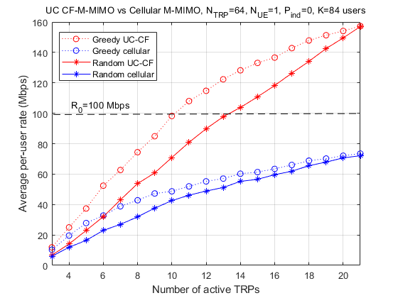
Figure 10: CF-M-MIMO vs Cellular adaptive switch-off rate performance when $K=84$ with hotspots.

Figure 9 depicts the EE performance, and reveals two important facts: 1) the CF-M-MIMO processing significantly outperforms the cellular M-MIMO counterpart; 2) the greedy switch-off technique provides a clear advantage over the random operation, with this gain being most visible in the CF-M-MIMO case. This is because carefully selecting the TRP to be switched-off allows some of the inherent rate loss associated to the switch-off to be compensated through the cooperation of nearby TRPs. In more details, when considering the CF-M-MIMO case, Alg. 2 achieves an EE of 1.5 Mbps/J with just $M=11$ active TRPs, whereas the random technique requires the full network ($M=21$) to only reach 1.25 Mbps/J.

Looking now at the rate performance when considering TRP shutdown in Figure 10, it is evident that CF-M-MIMO offers a clear advantage over cellular processing. From this figure, it can also be seen that Algorithm 2’s implementation of the greedy switch-off technique leads to a significant improvement in performance compared to using the random switch-off method. Cellular M-MIMO is not able to meet the UE rate constraint $R_{0}=100$ Mbps, also depicted in Fig. 10, while CF-M-MIMO can comfortably fulfill it by letting on $M\geq 10$ TRPs when using Algorithm 2 and $M\geq 14$ TRPs when using random switch-off. Also note that the switch-off of any TRP, independently of the technique in use, always results in a rate loss. However, when using Algorithm 2, this loss takes place more gracefully thanks to the cooperation between TRPs and the intelligent TRP switch-off. Remarkably, operating the network with $M=11$ TRPs results in a power consumption reduction of roughly 40% (from 10.1 kW to 6.1 kW) when compared to a network operating with all TRPs active.

Figure 11 assesses the performance of the proposed adaptive switch-off under different levels of power consumption while the TRPs is in shutdown for the specific case of $K=42$ UEs in the network and for different UE deployment conditions (i.e., $P_{ind}=0$ or $0.5$). In particular, and in accordance to [23], the power reduction coefficient is set to $\varpi=0.3,0.47$ and $0.7$, corresponding to symbol shutdown, carrier shutdown and dormancy, respectively. When focusing on the results for $P_{ind}=0$ —all UEs are outdoor—, increasing the power savings during shutdown increases the EE and reduces the optimum number of active TRPs. Note that to maximize EE, the optimum $M$ drops from 11 to 8 when transiting from symbol shutdown to dormancy savings. Although qualitatively the same can be said when $P_{ind}=0.5$, clearly the fact of having many indoor UEs causes both a drop in EE with respect to the all-outdoor UE case and the need for a larger number of active TRPs to maximize it.

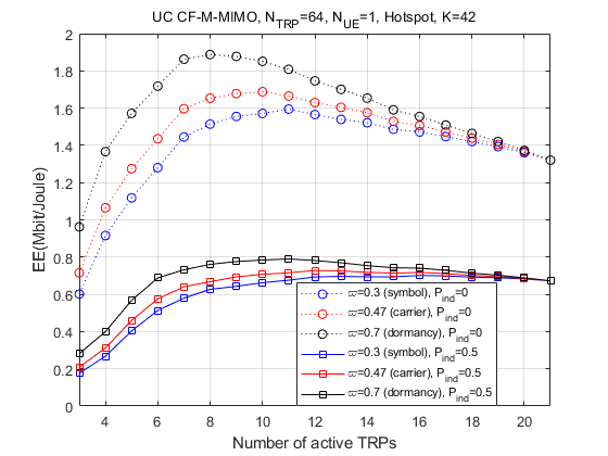
Figure 11: CF-M-MIMO EE for different fixed-power consumption factors when $K=42$.

VI-D Impact of inter-site distance

Finally, and in order to illustrate some of the of subtleties to be aware when implementing cell-free schemes, Fig. 12 re-evaluates the results in Fig. 10, but now considering an ISD of 500 meters. Note that this change implies more than quadrupling the coverage area while keeping the same number of TRPs and transmit power. The first important point to note is the clear degradation in terms of per-UE rate mainly caused by the larger propagation losses, which in turn renders the network unable to fulfill the $R_{0}=100$ Mbps target. It is remarkable that the difference between the greedy and random approaches become relatively much larger as the ISD becomes larger. This is because the switch-off of a TRPs makes its UEs to be served by other TRP that is farther away. Consequently, as the greedy technique is more effective in selecting the TRP to deactive than the random one, it causes less harm to the network performance. One more peculiar effect to be observed is that, for the random case, the purely cellular topology outperforms the CF-M-MIMO architecture when the number of active TRPs falls below 14 TRPs. The explanation for this effect has to be sought on the condition imposed on the CF-M-MIMO scheme that each TRP has to serve $K_{\text{TRP}}$ UEs. When only a few TRPs are active, certain UEs are served by TRPs that are extremely far away and barely provide any gain yet still induce strict power restrictions as shown in (12).

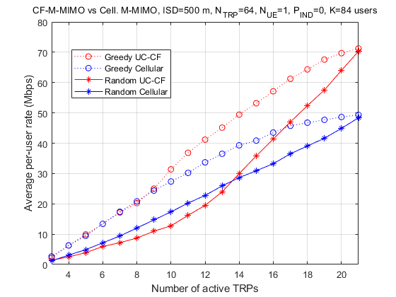
Figure 12: CF-M-MIMO vs Cellular adaptive switch-off rate performance when $K=84$ with hotspots and ISD =500 m.

VII Conclusion

This paper has quantified for the first time the energy and rate benefits of applying CF-M-MIMO processing to a state-of-the-art 5G macrocellular M-MIMO network, with large inter-site distances. It has been shown that the cell-free principle, even when applied to a regular topology, brings along large benefits in terms of increased SE when compared to conventional multicell M-MIMO architectures. This improvement is most substantial when serving outdoor UEs, whereas it is more modest when targeting indoor ones. Building on a recent and realistic 5G power consumption model, a novel mechanism has been proposed to selectively (and partially) switch on/off TRPs that provides major EE gains, often more than doubling that attained under classical cellular processing. It has been shown how multi-antenna UEs bring in new challenges due to the exacerbation of the pilot contamination phenomenon. In response, a novel strategy has been proposed that only allows those UEs with good propagation conditions to actually enjoy multi-stream transmission, while guaranteeing at the same time that UEs with poor channel conditions do not have their performance degraded due to an indiscriminate exploitation of the UE multi-antenna capabilities. Results show that the inherent performance loss associated to a TRP shutdown can be compensated by allowing nearby TRPs to cooperate using CF-M-MIMO processing. Future work will concentrate on the assessment of mixed topologies that combine arbitrarily placed TRPs equipped with few antennas with a single M-MIMO-equipped BS in an attempt to capitalize on the benefits of both architectures.

References

- [1] W. Jiang, B. Han, M. A. Habibi, and H. D. Schotten, “The road towards 6G: A comprehensive survey,” IEEE Open Journal of the Communications Society, vol. 2, pp. 334–366, 2021.
- [2] M. Matthaiou and et al., “The road to 6G: Ten physical layer challenges for communications engineers,” IEEE Communications Magazine, vol. 59, no. 1, pp. 64–69, 2021.
- [3] H. Tataria, M. Shafi, A. F. Molisch, M. Dohler, H. Sjöland, and F. Tufvesson, “6G wireless systems: Vision, requirements, challenges, insights, and opportunities,” Proceedings of the IEEE, vol. 109, no. 7, pp. 1166–1199, 2021.
- [4] M. A. Uusitalo, P. Rugeland, M. R. Boldi, E. C. Strinati, P. Demestichas, M. Ericson, G. P. Fettweis, M. C. Filippou, A. Gati, M.-H. Hamon et al., “6G vision, value, use cases and technologies from european 6G flagship project Hexa-X,” IEEE Access, vol. 9, pp. 160 004–160 020, 2021.
- [5] T. L. Marzetta, E. G. Larsson, H. Yang, and H. Q. Ngo, Fundamentals of massive MIMO. Cambridge Univ. Press, 2016.
- [6] D. López-Pérez, A. De Domenico, N. Piovesan, G. Xinli, H. Bao, S. Qitao, and M. Debbah, “A survey on 5G radio access network energy efficiency: Massive MIMO, lean carrier design, sleep modes, and machine learning,” IEEE Communications Surveys & Tutorials, 2022.
- [7] H. Q. Ngo, A. Ashikhmin, H. Yang, E. G. Larsson, and T. L. Marzetta, “Cell-free massive MIMO versus small cells,” IEEE Transactions on Wireless Communications, vol. 16, no. 3, pp. 1834–1850, 2017.
- [8] Ö. T. Demir, E. Björnson, and L. Sanguinetti, “Foundations of user-centric cell-free massive MIMO,” Foundations and Trends® in Signal Processing, vol. 14, no. 3-4, 2021.
- [9] T. C. Mai, H. Q. Ngo, and L.-N. Tran, “Energy efficiency maximization in large-scale cell-free massive mimo: A projected gradient approach,” IEEE Transactions on Wireless Communications, vol. 21, no. 8, pp. 6357–6371, 2022.
- [10] G. Femenias, N. Lassoued, and F. Riera-Palou, “Access point switch ON/OFF strategies for green cell-free massive MIMO networking,” IEEE Access, vol. 8, pp. 21 788–21 803, 2020.
- [11] J. García-Morales, G. Femenias, and F. Riera-Palou, “Energy-efficient access-point sleep-mode techniques for cell-free mmwave massive MIMO networks with non-uniform spatial traffic density,” IEEE Access, vol. 8, pp. 137 587–137 605, 2020.
- [12] I. Kanno, K. Yamazaki, Y. Kishi, and S. Konishi, “A survey on research activities for deploying cell free massive MIMO towards beyond 5G,” IEICE Transactions on Communications, p. 2021MEI0001, 2022.
- [13] T. Kim, H. Kim, S. Choi, and D. Hong, “How will cell-free systems be deployed?” IEEE Communications Magazine, vol. 60, no. 4, pp. 46–51, 2022.
- [14] T. C. Mai, H. Q. Ngo, and T. Q. Duong, “Downlink spectral efficiency of cell-free massive mimo systems with multi-antenna users,” IEEE Transactions on Communications, vol. 68, no. 8, pp. 4803–4815, 2020.
- [15] M. Series, “Guidelines for evaluation of radio interface technologies for IMT-2020,” Report ITU, pp. 2412–0, 2017.
- [16] A. Checko, H. L. Christiansen, Y. Yan, L. Scolari, G. Kardaras, M. S. Berger, and L. Dittmann, “Cloud RAN for mobile networks-a technology overview,” IEEE Communications surveys & Tutorials, vol. 17, no. 1, pp. 405–426, 2014.
- [17] E. Björnson and L. Sanguinetti, “Scalable cell-free massive MIMO systems,” IEEE Transactions on Communications, vol. 68, no. 7, pp. 4247–4261, 2020.
- [18] 3GPP, “Study on 3D channel model for LTE (Release 12),” 3GPP TR 36.873 (version 12.7.0), December 2017.
- [19] E. Björnson, J. Hoydis, and L. Sanguinetti, “Massive MIMO networks: Spectral, energy, and hardware efficiency,” Foundations and Trends® in Signal Processing, vol. 11, no. 3-4, 2017.
- [20] G. Femenias and F. Riera-Palou, “Cell-free millimeter-wave massive MIMO systems with limited fronthaul capacity,” IEEE Access, vol. 7, pp. 44 596–44 612, 2019.
- [21] S. M. Kay, Fundamentals of statistical signal processing: estimation theory. Prentice-Hall, Inc., 1993.
- [22] E. Björnson and L. Sanguinetti, “Making cell-free massive MIMO competitive with MMSE processing and centralized implementation,” IEEE Transactions on Wireless Communications, vol. 19, no. 1, pp. 77–90, 2019.
- [23] N. Piovesan, D. Lopez-Perez, A. De Domenico, X. Geng, H. Bao, and M. Debbah, “Machine learning and analytical power consumption models for 5G base stations,” IEEE Communications Magazine, vol. 60, no. 10, pp. 56–62, 2022.
- [24] S. Chen, J. Zhang, E. Björnson, Ö. T. Demir, and B. Ai, “Energy-efficient cell-free massive MIMO through sparse large-scale fading processing,” arXiv preprint arXiv:2208.13552, 2022.
- [25] X. Li, E. Björnson, S. Zhou, and J. Wang, “Massive mimo with multi-antenna users: When are additional user antennas beneficial?” in 2016 23rd International Conference on Telecommunications (ICT). IEEE, 2016, pp. 1–6.
- [26] F. Riera-Palou, G. Femenias, J. García-Morales, and H. Q. Ngo, “Selective infrastructure activation in cell-free massive MIMO: a two time-scale approach,” in 2021 IEEE Globecom Workshops (GC Wkshps). IEEE, 2021, pp. 1–7.
- [27] F. Riera-Palou, G. Femenias, A. G. Armada, and A. Pérez-Neira, “Clustered cell-free massive MIMO,” in 2018 IEEE Globecom Workshops (GC Wkshps). IEEE, 2018, pp. 1–6.
- [28] 3GPP, “Technical specification group radio access network; evolved universal terrestrial radio access (E-UTRA); further advancements for E-UTRA physical layer aspects (release 9),” 3GPP TR 36.814 (version 9.2.0), December 2017.