A Single-Loop Deep Actor-Critic Algorithm for Constrained Reinforcement Learning with Provable Convergence

Abstract

Deep Actor-Critic algorithms, which combine Actor-Critic with deep neural network (DNN), have been among the most prevalent reinforcement learning algorithms for decision-making problems in simulated environments. However, the existing deep Actor-Critic algorithms are still not mature to solve realistic problems with non-convex stochastic constraints and high cost to interact with the environment. In this paper, we propose a single-loop deep Actor-Critic (SLDAC) algorithmic framework for general constrained reinforcement learning (CRL) problems. In the actor step, the constrained stochastic successive convex approximation (CSSCA) method is applied to handle the non-convex stochastic objective and constraints. In the critic step, the critic DNNs are only updated once or a few finite times for each iteration, which simplifies the algorithm to a single-loop framework (the existing works require a sufficient number of updates for the critic step to ensure a good enough convergence of the inner loop for each iteration). Moreover, the variance of the policy gradient estimation is reduced by reusing observations from the old policy. The single-loop design and the observation reuse effectively reduce the agent-environment interaction cost and computational complexity. In spite of the biased policy gradient estimation incurred by the single-loop design and observation reuse, we prove that the SLDAC with a feasible initial point can converge to a Karush-Kuhn-Tuker (KKT) point of the original problem almost surely. Simulations show that the SLDAC algorithm can achieve superior performance with much lower interaction cost.

I Introduction

Reinforcement learning (RL) has been successfully applied to many sequential decision-making problems, such as playing Go [1], robot locomotion, and manipulation [2]. The agent learns to act by trial and error freely in a simulated environment, as long as it brings performance improvement. However, in many realistic domains such as Question-answering systems for medical emergencies [3] and radio resource management (RRM) in future 6G wireless communications [4], there are complicated stochastic constraints and the cost for an agent to interact with the environment is high. For example, the RRM in wireless communications needs to satisfy various quality of services (QoS) requirements such as average throughput and delay, which usually belong to non-convex stochastic constraints. Moreover, each interaction with the wireless environment involves channel estimation and/or data transmission over wireless channels, which is quite resource-consuming. Naturally, the huge commercial interest in deploying the RL agent to realistic domains motivates the study of constrained reinforcement learning (CRL) with as few agent-environment interactions as possible.

A standard and well-studied formulation for the CRL problem mentioned above is the constrained Markov Decision Process (CMDP) framework [5]. In a CMDP framework, the agent attempts to maximize its expected total reward while also needs to ensure constraints on expectations of auxiliary costs. Together with the stochasticity and the non-convexity of objective function and constraints over the infinite-dimensional policy space, it is not a trivial task to solve the CMDP, and the existing algorithms for CMDP are still far from mature. The major lines of research on this topic can be divided into the following three categories.

Actor-only methods: Such methods work with a parameterized family of policies, and the gradient of the actor parameters is directly estimated by simulation [6, 7]. However, a common drawback of Actor-only methods is that the gradient estimators may have a large variance [8]. For example, authors in [9] propose a successive convex approximation based off-policy optimization (SCAOPO) algorithm to solve CRL problems, and the Q values involved in the gradient estimation are given by Monte Carlo (MC) method. However, the MC method always finds the estimates that minimize mean-squared error on the training set [10], and thus its performance depends heavily on the batch size of the sample, which incurs a long convergence time, especially when observations are sparse.

Critic-only methods: Unlike Actor-only methods, such methods only focus on value function approximation rather than optimizing over the policy space directly. For example, the authors of [11] propose a fuzzy constraint Q-learning algorithm to learn the optimal route for vehicular ad hoc networks. However, a method of this type may succeed in constructing a “good” approximation of the value function yet lack reliable guarantees in terms of near-optimality of the resulting policy [12].

Actor-Critic methods: Methods of this type aim at combining the advantages of actor-only and critic-only methods, which is the primary focus of this paper. In each iteration of Actor-Critic algorithms, the actor is updated in an approximate gradient direction using the action-value function provided by the critic, and the critic simultaneously updates its parameters using policy evaluation algorithms. Some representative studies for unconstrained cases can be found in [13, 14]. However, to the best of our knowledge, none of the existing Actor-Critic methods have a theoretical guarantee of convergence to KKT points of the general CMDP, or even the convergence to a feasible point. Taking into account the constrained cases, one common approach is to relax the constraints via Lagrangian multipliers and formulated an unconstrained saddle-point optimization problem, such as trust region policy optimization-Lagrangian (TRPO-Lag) and proximal policy optimization-Lagrangian (PPO-Lag) [15]. However, these primal-dual optimization (PDO) methods are sensitive to the initialization of the dual variable $\lambda$, which needs to be carefully picked to attain the desired trade-off between reward and constraint cost. Authors in [16] propose the constrained policy optimization (CPO) algorithm, which updates the policy within a trust-region framework. Nevertheless, due to the non-convexity and high computation complexity, the CPO introduces some approximate operations at the cost of sacrificing the stable performance [17] and also cannot theoretically assure a strictly feasible result. Moreover, all the existing works mentioned above adopt the stochastic gradient descent (SGD) method to update policy in the actor step, which makes them only suitable for simple constraints where the feasible set can be represented by a deterministic convex set.

To handle large state and action spaces, modern algorithms often parameterize both the policy and the action-value function with deep neural networks (DNN) [18], namely, deep Actor-Critic, which incurs non-convexity on both the objective function and feasible region. The above restrictions of existing works hinder us from better diagnosing the possible failure and applying deep Actor-Critic to realistic domains. In addition, the existing Actor-Critic algorithms have a high cost to interact with the environment. One reason for this is the two-loop framework design. For example, [19] shows that the Proximal Policy Optimization algorithm for unconstrained RL problems can converge to the globally optimal policy at sub-linear rates, but under the unrealistic assumption that the action-value can be exactly estimated through infinite inner iterations. Considering the discounted reward setting, [20] establishes the global convergence of TRPO for unconstrained cases, but requires that the parameters of the action-value function (Q function) be updated a sufficient number of times to ensure a good enough convergence of the inner loop at each iteration, which results in the high complexity and slow convergence. Another reason for the high interaction cost is that all the above existing Actor-Critic algorithms have assumed episodic tasks with on-policy sampling, and the agent is able to generate arbitrary long trajectories of observations to compute estimates at each iteration. However, the engineering systems/environments usually cannot be manipulated at will, and the data sampling is not free in the real world.

To combat these weaknesses above, we propose a single-loop deep Actor-Critic (SLDAC) algorithm for constrained reinforcement learning problems in this paper. To attain prominent performance, both the policy and the Q functions in SLDAC are parameterized by DNN. In the actor step, the policy is optimized by the constrained stochastic successive convex approximation (CSSCA) algorithm [21], which can find a stationary point for a general non-convex constrained stochastic optimization problem. In the critic step, to reduce the agent-environment interaction cost and computational complexity, we update the critic DNNs only once by the Temporal-Difference (TD) learning method at each iteration and estimate the policy gradient by reusing observations from the old policy. We adopt the single-loop framework based on the intuition that the critic DNNs do not have to accurately estimate the true value functions within each iteration, as long as the critic DNNs keep “learning” faster than the actor DNN, both DNNs can attain optimum simultaneously. In practice, we can also perform the critic step a few finite times to attain a good trade-off between performance and complexity/interaction cost. However, the single-loop design and the observation reuse in the critic step incur biased estimation of action-value functions and policy gradients, and with the coupling of the actor step and the critic step, it becomes non-trivial to establish the theoretical guarantee of algorithm convergence. Nonetheless, we manage to prove that SLDAC can still converge to a Karush-Kuhn-Tuker (KKT) point of the original problem almost surely with a feasible initial point. The main contributions are summarized below.

• First Single-Loop Deep Actor-Critic for CMDP: We propose SLDAC, the first deep Actor-Critic variant for general CMDPs with non-convex stochastic constraints. In contrast to prior works, there are two major differences/advantages: 1) our method takes into account the stochasticity and the non-convexity of both the objective function and the constraints; 2) the combination of single-loop framework and off-policy optimization reusing old observations can significantly reduce the agent-environment interaction cost and computational complexity.

• Theoretical Convergence Analysis of SLDAC: We establish an asymptotic convergence analysis for SLDAC, despite the challenges posed by the single-loop design, the observation reuse, and the coupling of the critic and actor steps.

The rest of the paper is organized as follows. Section II briefly introduces some preliminaries, including general formulations of CRL, neural network parameterization, and assumptions on problem structure. The SLDAC algorithmic framework and its convergence analysis are presented in Sections III and IV, respectively. Section V provides simulation results and the conclusion is drawn in section VII.

II Preliminaries

In this section, we first lay out the formulation of general CRL problems and then briefly introduce a family of deep ReLU neural networks, which are commonly used in modern algorithms to parameterize the policy $\pi$ and Q-functions. Moreover, we make several assumptions on the problem structure, before we present the algorithmic framework.

II-A Problem Formulation

We first introduce some preliminaries of CMDP, which is an MDP with additional constraints that restrict the set of allowable policies. A CMDP is denoted by a tuple $\left(\mathcal{S},\mathcal{\mathcal{A}},P,C\right)$, where $\mathcal{S}\subseteq\mathbb{R}^{n_{\boldsymbol{s}}}$ and $\mathcal{\mathcal{A}}\subseteq\mathbb{R}^{n_{\boldsymbol{a}}}$ are state space and action space respectively, $P:\mathcal{S}\times\mathcal{A}\times\mathcal{S}\rightarrow\left[0,1\right]$ is the transition probability function, with $P\left(\boldsymbol{s}^{\prime}\mid\boldsymbol{s},\boldsymbol{a}\right)$ denoting the probability of transition to state $\boldsymbol{s}^{\prime}$ from the previous state $\boldsymbol{s}\in\mathcal{S}$ with an action $\boldsymbol{a}\in\mathcal{\mathcal{A}}$, $C_{0}:\mathcal{S}\times\mathcal{A}\rightarrow\mathbb{R}$ is the per-stage cost function, and $C_{1},\ldots,C_{I}$ with each one $C_{i}:\mathcal{S}\times\mathcal{A}\rightarrow\mathbb{R}$ are the per-stage constraint functions. The policy $\pi:\mathcal{S}\rightarrow\mathbf{P}\left(\mathcal{A}\right)$ is a map from states to probability distributions, with $\pi\left(\boldsymbol{a}\mid\boldsymbol{s}\right)$ denoting the probability of selecting action $\boldsymbol{a}\in\mathcal{A}$ in state $\boldsymbol{s}\in\mathcal{S}$. Let $\boldsymbol{s}_{t}$ and $\boldsymbol{a}_{t}$ denote the state and action at time step $t$, then the transition probability $P$ and policy $\pi$ determine the probability distribution of the trajectory $\left\{\boldsymbol{s}_{0},\boldsymbol{a}_{0},\boldsymbol{s}_{1},\ldots\right\}$. For notational simplicity, we denote the distribution over the trajectories under policy $\pi$ by $p_{\pi}$, i.e., $\boldsymbol{s}_{t}\thicksim P\left(\cdot\mid\boldsymbol{s}_{t-1},\boldsymbol{a}_{t-1}\right),\boldsymbol{a}_{t}\thicksim\pi\left(\cdot\mid\boldsymbol{s}_{t}\right)$.

Because of the curse of dimension, we parameterize the policy $\pi$ with DNN over $\boldsymbol{\theta}\in\mathbf{\Theta}$, and then we denote the parameterized policy as $\pi_{\boldsymbol{\theta}}$. With the $\pi_{\boldsymbol{\theta}}$, the goal of a general CRL problem can be formulated based on the CMDP as:

$$\underset{\theta\in\Theta}{\mathrm{min}}J_{0}\left(\boldsymbol{\theta}\right)\overset{\triangle}{=} \underset{T\rightarrow\infty}{\mathrm{lim}}\frac{1}{T}\mathbb{E}_{p_{\pi_{\boldsymbol{\theta}}}}\left[\stackrel{{\scriptstyle[}}{{t}}=0]{T-1}{\sum}C_{0}\left(\boldsymbol{s}_{t},\boldsymbol{a}_{t}\right)\right]$$ (1)

$$\mathrm{s.t.}J_{i}\left(\boldsymbol{\theta}\right)\overset{\triangle}{=} \underset{T\rightarrow\infty}{\mathrm{lim}}\frac{1}{T}\mathbb{E}_{p_{\pi_{\boldsymbol{\theta}}}}\left[\stackrel{{\scriptstyle[}}{{t}}=0]{T-1}{\sum}C_{i}\left(\boldsymbol{s}_{t},\boldsymbol{a}_{t}\right)\right]-c_{i}\leq 0.$$

where $c_{1},\ldots,c_{I}$ denote the constraint values. Problem (1) embraces many important applications, and we give two examples in the following, which has also been considered in [9].

Example 1 (Delay-Constrained Power Control for Downlink Multi-User MIMO (MU-MIMO) system)

Consider a downlink MU-MIMO system consisting of a base station (BS) equipped with $N_{t}$ antennas and $K$ single-antenna users ($N_{t}\geq K$), where the BS maintains $K$ dynamic data queues for the burst traffic flows to each user. Suppose that the time dimension is partitioned into decision slots indexed by $t$ with slot duration $t_{0}$, and each queue dynamic of the $k$-user has a random arrival data rate $A_{k}\left(t\right)$, where $E\left[A_{k}\right]=\lambda_{k}$. The data rate $R_{k}\left(t\right)$ of user $k$ is given by

$$R_{k}=B\mathrm{log}_{2}\left(1+\frac{P_{k}\bigl{|}\boldsymbol{h}_{k}^{H}\boldsymbol{v}_{k}\left(\alpha_{Z}\right)\bigr{|}^{2}}{\sum_{j\neq k}P_{j}\bigl{|}\boldsymbol{h}_{k}^{H}\boldsymbol{v}_{k}\left(\alpha_{Z}\right)\bigr{|}^{2}+\sigma_{k}^{2}}\right),$$

where we omit the time slot index for conciseness, $B$ denotes the bandwidth, $\boldsymbol{h}_{k}$ is the downlink channel of the $k$-th user, $\sigma_{k}^{2}$ is the noise power at the $k$-th user, $P_{k}$ is the power allocated to the $k$-th user and $\boldsymbol{v}_{k}\left(\alpha_{Z}\right)$ is the normalized regularized zero-forcing (RZF) precoder with regularization factor $\alpha_{Z}$ [22]. Then the queue dynamic of the $k$-user $Q_{k}\left(t\right)$ is given by

$$Q_{k}\left(t\right)=\mathrm{max}\Bigl{\{}A_{k}\left(t\right)t_{0}-R_{k}\left(t\right)t_{0}+Q_{k}\left(t-1\right),0\Bigr{\}}.$$

In this case, the BS at the $t$-th time slot obtains state information $\boldsymbol{s}_{t}=\left\{\mathbf{Q}\left(t\right),\mathbf{H}\left(t\right)\right\}$, where $\mathbf{Q}=\left[Q_{1},\ldots,Q_{K}\right]^{\top}\in\mathbb{R}^{K}$ and $\mathbf{H}=\left[\boldsymbol{h}_{1},\ldots,\boldsymbol{h}_{K}\right]^{H}\in C^{K\times N_{t}}$, and takes action $\boldsymbol{a}_{t}=\left\{\boldsymbol{P}_{t}\left(t\right),\alpha_{Z}\left(t\right)\right\}$ according to policy $\pi_{\boldsymbol{\theta}}$, where $\boldsymbol{P}_{t}=\left[P_{1},\ldots,P_{K}\right]$. The objective of the delay-constrained power control problem is to obtain a policy $\pi_{\boldsymbol{\theta}}$ that minimizes the long-term average power consumption as well as satisfying the average delay constraint for each user, which can be formulated as

$$\underset{\theta\in\Theta}{\mathrm{min}}J_{0}\left(\boldsymbol{\theta}\right)\overset{\triangle}{=} \underset{T\rightarrow\infty}{\mathrm{lim}}\frac{1}{T}\mathbb{E}_{p_{\pi_{\boldsymbol{\theta}}}}\left[\stackrel{{\scriptstyle[}}{{t}}=1]{T}{\sum}\stackrel{{\scriptstyle[}}{{k}}=1]{K}{\sum}P_{k}\left(t\right)\right]$$ (2)

$$\mathrm{s.t.}J_{i}\left(\boldsymbol{\theta}\right)\overset{\triangle}{=} \underset{T\rightarrow\infty}{\mathrm{lim}}\frac{1}{T}\mathbb{E}_{p_{\pi_{\boldsymbol{\theta}}}}\left[\stackrel{{\scriptstyle[}}{{t}}=1]{T}{\sum}\frac{Q_{k}\left(t\right)}{\lambda_{k}}\right]-c_{k}\leq 0,\forall k,$$

where $c_{1},\ldots,c_{K}$ denote the maximum allowable average delay for each user.

Example 2 (Constrained Linear-Quadratic Regulator)

Linear-quadratic regulator (LQR) is one of the most fundamental problems in control theory [23]. We denote $\boldsymbol{s}_{t}\in\mathbb{R}^{n_{\boldsymbol{s}}}$ and $\boldsymbol{a}_{t}\in\mathbb{R}^{n_{\boldsymbol{a}}}$ as the state and action of LQR problem at the time $t$, respectively. Then according to [24], the cost $C_{0}\left(\boldsymbol{s}_{t},\boldsymbol{a}_{t}\right)$ and the rule that maps the current state and control action to a new state can be given by

$$C_{0}\left(\boldsymbol{s}_{t},\boldsymbol{a}_{t}\right)=\boldsymbol{s}_{t}^{\mathrm{T}}Q_{0}\boldsymbol{s}_{t}+\boldsymbol{a}_{t}^{\mathrm{T}}R_{0}\boldsymbol{a}_{t},$$ (3)

$$\boldsymbol{s}_{t+1}=\mathbf{X}\boldsymbol{s}_{t}+\mathbf{Y}\boldsymbol{a}_{t}+\epsilon_{t},$$ (4)

where $\mathbf{X}\in\mathbb{R}^{n_{\boldsymbol{s}}\times n_{\boldsymbol{a}}}$ and $\mathbf{Y}\in\mathbb{R}^{n_{\boldsymbol{s}}\times n_{\boldsymbol{a}}}$ are transition matrices, $\left\{\epsilon_{t}\right\}$ is the process noise and $Q_{0}\in\mathbb{R}^{n_{\boldsymbol{s}}\times n_{\boldsymbol{a}}}$ and $R_{0}\in\mathbb{R}^{n_{\boldsymbol{a}}\times n_{\boldsymbol{a}}}$ are cost matrices. Furthermore, the aim of constrained LQR can be formulated the same as (1).

II-B Neural Network Parameterization

Following the same standard setup implemented in line of recent works [25], [26], and [27], we consider such an $L$-hidden-layer neural network:

$$f_{m}\left(\boldsymbol{\alpha};\boldsymbol{x}\right)=\sqrt{m}\mathbf{W}_{L}\sigma\left(\mathbf{W}_{L-1}\cdots\sigma\left(\mathbf{W}_{1}\boldsymbol{\phi}\bigl{(}\boldsymbol{x}\bigr{)}\right)\cdots\right),$$ (5)

where $m$ is the width of the neural network, $\sigma\left(\cdot\right)$ is the entry-wise activation function, $\boldsymbol{\phi}\bigl{(}\cdot\bigr{)}$ is a feature mapping of the input data $\boldsymbol{x}\in\mathbb{R}^{d}$, and the input data is usually normalized, i.e., $\left\|\boldsymbol{x}\right\|_{2}\leq 1$. Moreover, $\mathbf{W}_{1}\in\mathbb{R}^{m\times d_{\mathrm{in}}}$, $\mathbf{W}_{L}\in\mathbb{R}^{d_{\mathrm{out}}\times m}$ and $\mathbf{W}_{l}\in\mathbb{R}^{m\times m}$ for $l=2,\ldots,L-1$ are parameter matrices, and $\boldsymbol{\alpha}=\left(\mathrm{vec}\left(\mathbf{W}_{1}\right)^{\mathrm{\intercal}},\ldots,\mathrm{vec}\left(\mathbf{W}_{L}\right)^{\mathrm{\intercal}}\right)$ is the concatenation of the vectorization of all the parameter matrices. It is easy to verify that $\bigl{\|}\boldsymbol{\alpha}-\boldsymbol{\alpha}^{\prime}\bigr{\|}_{2}^{2}=\sum_{l=1}^{L}\bigl{\|}\mathbf{W}_{l}-\mathbf{W}_{l}^{{}^{\prime}}\bigr{\|}_{F}^{2}$. In this paper, we only consider the most commonly used activation function rectified linear unit (ReLU), i.e. $\sigma\left(z\right)=\mathrm{max}\bigl{\{}z,0\bigr{\}}$, and for simplicity, we assume that the width $m$ of different layers in a network are the same. Remark that our result can be easily generalized to many other activation functions and the setting that the widths of each layer are not equal but in the same order, which is discussed in [28] and [29].

In this paper, we parameterize both the policy and Q-functions with the DNNs defined above to facilitate rigorous convergence analysis. However, the proposed algorithm also works for other types of DNNs. In the actor step, we employ the commonly used Gaussian policy [30, Chapter 13.7] with mean $\boldsymbol{\mu}$ and diagonal elements of the covariance matrix $\mathbf{\Sigma}$ parameterized by $f_{m_{\boldsymbol{\mu}}}\bigl{(}\boldsymbol{\theta}_{\boldsymbol{\mu}};\boldsymbol{s}\bigr{)}=\mathbb{R}^{n_{\boldsymbol{a}}}$ and $f_{m_{\boldsymbol{\sigma}}}\bigl{(}\boldsymbol{\theta}_{\boldsymbol{\sigma}};\boldsymbol{s}\bigr{)}\subseteq\mathbb{R}^{n_{\boldsymbol{a}}}$, respectively, and keep the non-diagonal elements of $\mathbf{\Sigma}$ as $0$. That is,

$$\pi_{\boldsymbol{\theta}}\left(\boldsymbol{a}\mid\boldsymbol{s}\right)\propto\left|\mathbf{\Sigma}\right|^{\text{$-\frac{1}{2}$}}\mathrm{exp}\Bigl{(}-\frac{1}{2}\bigl{(}\boldsymbol{\mu}-\boldsymbol{a}\bigr{)}^{\intercal}\mathbf{\Sigma}^{-1}\bigl{(}\boldsymbol{\mu}-\boldsymbol{a}\bigr{)}\Bigr{)},$$ (6)

where the policy parameter $\boldsymbol{\theta}=\bigl{[}\boldsymbol{\theta}_{\boldsymbol{\mu}},\boldsymbol{\theta}_{\boldsymbol{\sigma}}\bigr{]}\in\mathbf{\Theta}$. In the critic step, for each cost (reward) function, we adopt dual critic DNNs $f_{m_{Q}}\left(\boldsymbol{\omega}^{i};\boldsymbol{s},\boldsymbol{a}\right)\subseteq\mathbb{R}$ and $f_{m_{Q}}\left(\bar{\boldsymbol{\omega}}^{i};\boldsymbol{s},\boldsymbol{a}\right)\subseteq\mathbb{R}$ to approximate it, with parameters $\boldsymbol{\omega}^{i},\bar{\boldsymbol{\omega}}^{i}\in\Omega_{i}$, the details of which will be provided in Section III-A. For simplification, we assume the same DNNs (but with different critic DNN parameters $\boldsymbol{\omega}$ are used to approximate different Q functions. In addition, we abbreviate $f_{m_{Q}}\left(\boldsymbol{\omega};\boldsymbol{s},\boldsymbol{a}\right)$ to $f\left(\boldsymbol{\omega}\right)$ throughout this paper when no confusion arises.

II-C Important Assumptions on the Problem Structure

Assumption 1.

(Assumptions on the Problem Structure)
1) There are constants $\lambda>0$ and $\rho\in\left(0,1\right)$ satisfying

$$\mathrm{sup}_{\boldsymbol{s}\in\mathcal{S}}d_{TV}\left(\mathbf{P}\left(\boldsymbol{s}_{t}\mid\boldsymbol{s}_{0}=\boldsymbol{s}\right),\mathbf{P_{\pi_{\boldsymbol{\theta}}}}\right)\leq\lambda\rho^{t},$$ (7)

for all $t=0,1,\cdots$, where $\mathbf{P_{\pi_{\boldsymbol{\theta}}}}$ is the stationary state distribution under policy $\pi_{\boldsymbol{\theta}}$ and $d_{TV}\left(\mu,v\right)=\int_{\boldsymbol{s}\in\mathcal{S}}\left|\mu\left(\mathrm{d}\boldsymbol{s}\right)-v\left(\mathrm{d}\boldsymbol{s}\right)\right|$ denotes the total-variation distance between the probability measures $\mu$ and $v$.
2) State space $\mathcal{S}\subseteq\mathbb{R}^{n_{\boldsymbol{s}}}$ and action space $\mathcal{A}\subseteq\mathbb{R}^{n_{\boldsymbol{a}}}$ are both compact.
3) The cost/reward $C_{i},\forall i$, the derivative and the second-order derivative of $J_{i}\left(\boldsymbol{\theta}\right)$ are uniformly bounded.
4) The DNNs’ parameter spaces $\mathbf{\Theta}\subseteq\mathbb{R}^{n_{\boldsymbol{\theta}}}$ and $\Omega_{i}\subseteq\mathbb{R}^{n_{\boldsymbol{\omega}}},\forall i$ are compact and convex, and the outputs of DNNs are bounded.
5) The policy $\pi_{\boldsymbol{\theta}}$ follows Lipschitz continuity over the parameter $\boldsymbol{\theta}\in\mathbf{\Theta}$.

Assumption 1-1) controls the bias caused by the Markovian noise in the observations by assuming the uniform ergodicity of the Markov chain generated by $\pi_{\boldsymbol{\theta}}$, which is a standard requirement in the literature, see e.g., [31], [32] and [9]. Assumption 1-2) considers a general scenario in which the state and action spaces can be continuous. Assumption 1-3) indicates that the Lipschitz continuity of $\left\{J_{i}\left(\boldsymbol{\theta}\right)\right\}_{i=0,\ldots I}$ over parameters $\boldsymbol{\theta}$, which is usually assumed in the rigorous convergence analysis of RL algorithms [33, 34]. Assumption 1-4) is trivial in CRL problems. Assumption 1-5) indicates that the gradient of the policy DNN is always finite, which can be easily satisfied as long as the input and the width $m_{\boldsymbol{\mu}},m_{\boldsymbol{\sigma}}$ are bounded according to [27].

III SLDAC Algorithmic Framework

III-A Summary of SLDAC Algorithm

Based on the Actor-Critic framework, the proposed SLDAC algorithm performs iterations between the update of the critic network and the update of the actor network until convergence. The critic step attempts to find an approximation of the Q-functions, and then calculate the policy gradients at the $t$-th iteration, which are required by the construction of surrogate functions in the actor step. The actor step performs the CSSCA algorithm, which is based on solving a sequence of convex objective/feasibility optimization problems obtained by replacing the objective and constraint functions with surrogate functions. We will elaborate on it in the following, and finally, the overall SLDAC algorithm is summarized in Algorithm 1.

III-A1 The Critic Step

Given the current policy $\pi_{\boldsymbol{\theta}_{t}}$, the agent at state $\boldsymbol{s}_{t}$ chooses an action $\boldsymbol{a}_{t}$ according to the policy $\pi_{\boldsymbol{\theta}_{t}}$ and transitions to the next new state $\boldsymbol{s}_{t+1}$ with the environment feeding back a set of cost (reward) function values $\left\{C_{i}^{\text{'}}(\boldsymbol{s}_{t},\boldsymbol{a}_{t})\right\}_{i=0,\ldots,I}$, where $C_{0}^{\text{'}}(\boldsymbol{s}_{t},\boldsymbol{a}_{t})=C_{0}(\boldsymbol{s}_{t},\boldsymbol{a}_{t})$ and $C_{i}^{\text{'}}(\boldsymbol{s}_{t},\boldsymbol{a}_{t})=C_{i}(\boldsymbol{s}_{t},\boldsymbol{a}_{t})-c_{i},i=1,\ldots,I$. We denote the new observation as $\varepsilon_{t}=\left\{\boldsymbol{s}_{t},\boldsymbol{a}_{t},\left\{C_{i}^{\text{'}}(\boldsymbol{s}_{t},\boldsymbol{a}_{t})\right\}_{i=0,\ldots,I},\boldsymbol{s}_{t+1}\right\}$.

For any $\pi_{\boldsymbol{\theta}_{t}}$, correspondingly, there is a set of exact Q-functions$\left\{Q_{i}^{\pi_{\boldsymbol{\theta}_{t}}}\right\}_{i=0,,\ldots I}$ defined as

$$Q_{i}^{\pi_{\boldsymbol{\theta}_{t}}}\left(\boldsymbol{s},\boldsymbol{a}\right)= \mathbb{E}_{p_{t}}\Bigl{[}\sum_{l=0}^{\infty}\Bigl{(}C_{i}^{\text{'}}(\boldsymbol{s}_{l},\boldsymbol{a}_{l})-J_{i}\left(\boldsymbol{\theta}_{t}\right)\Bigr{)}$$

$$\Bigr{|}\boldsymbol{s}_{0}=\boldsymbol{s},\boldsymbol{a}_{0}=\boldsymbol{a}\Bigr{]},\forall i,\boldsymbol{s},\boldsymbol{a},$$ (8)

where we denote the state-action distribution $p_{\pi_{\boldsymbol{\theta}_{t}}}$ by $p_{t}$ for short. However, it is unrealistic to obtain $J_{i}\left(\boldsymbol{\theta}_{t}\right)$ online, so we redefine approximate Q-functions $\hat{Q}_{i}^{\pi_{\boldsymbol{\theta}_{t}}},\forall i$:

$$\hat{Q}_{i}^{\pi_{\boldsymbol{\theta}_{t}}}\left(\boldsymbol{s},\boldsymbol{a}\right)= \mathbb{E}_{p_{t}}\Bigl{[}\sum_{l=0}^{\infty}\Bigl{(}C_{i}^{\text{'}}(\boldsymbol{s}_{l},\boldsymbol{a}_{l})-\hat{J}_{i}^{t}\Bigr{)}$$

$$\Bigr{|}\boldsymbol{s}_{0}=\boldsymbol{s},\boldsymbol{a}_{0}=\boldsymbol{a}\Bigr{]},\forall i,\boldsymbol{s},\boldsymbol{a},$$ (9)

where $\hat{J}_{i}^{t}$ is the estimate of $J_{i}\left(\boldsymbol{\theta}_{t}\right)$ that will be given in (17). Later we will show that $\lim_{t\rightarrow\infty}\bigl{|}\hat{J}_{i}^{t}-J_{i}\bigl{(}\boldsymbol{\theta}_{t}\bigr{)}\bigr{|}=0$ and thus the estimate is asymptotically accurate.

First, we adopt a set of critic networks $\left\{f\left(\boldsymbol{\omega}^{i}\right)\right\}_{i=0,\ldots,I}$ defined in Section II-B to approximate $\hat{Q}_{i}^{\pi_{\boldsymbol{\theta}_{t}}},\forall i$ according to the new observation $\varepsilon_{t}$, which leads to minimizing the mean-squared projected Bellman error (MSBE) [31]:

$$\underset{\boldsymbol{\omega}_{t}^{i}}{\mathrm{min}}\ \mathbb{E}_{\sigma_{\pi_{\boldsymbol{\theta}_{t}}}}\Bigl{[}\Bigl{(}f\left(\boldsymbol{\omega}_{t}^{i};\boldsymbol{s}_{t},\boldsymbol{a}_{t}\right)-\mathcal{T}_{t}\ f\left(\boldsymbol{\omega}_{t}^{i};\boldsymbol{s}_{t},\boldsymbol{a}_{t}\right)\Bigr{)}^{2}\Bigr{]},\forall i,$$ (10)

where $\sigma_{\pi_{\boldsymbol{\theta}_{t}}}\left(\boldsymbol{s}_{t},\boldsymbol{a}_{t}\right)=\pi_{\boldsymbol{\theta}_{t}}\left(\boldsymbol{a}_{t}\mid\boldsymbol{s}_{t}\right)\cdot\mathbf{P_{\pi}}\left(\boldsymbol{s}_{t}\right)$ is the stationary state-action distribution, and we abbreviate it as $\sigma_{t}$. In addition, the Bellman operator $\mathcal{T}_{t}$ is defined as

$$\mathcal{T}_{t}\ f\left(\boldsymbol{\omega}_{t}^{i};\boldsymbol{s}_{t},\boldsymbol{a}_{t}\right)= \mathbb{E}_{p_{t}}\Bigl{[}f\left(\boldsymbol{\omega}_{t}^{i};\boldsymbol{s}_{t+1},\boldsymbol{a}_{t+1}^{\prime}\right)\Bigr{]}$$ (11)

$$+C_{i}^{\text{'}}(\boldsymbol{s}_{t},\boldsymbol{a}_{t})-\hat{J}_{i}^{t},\forall i,$$

where $\boldsymbol{a}_{t+1}^{\prime}$ is the action chosen by current policy $\pi_{\boldsymbol{\theta}_{t}}$ at the next state $\boldsymbol{s}_{t+1}$. To solve Problem (10), we first define a neighborhood of the randomly initialized parameter $\boldsymbol{\omega}_{0}^{i},\forall i$ as

$$\mathbb{B}\left(\boldsymbol{\omega}_{0}^{i},R_{\boldsymbol{\omega}}\right)= \Bigl{\{}\boldsymbol{\omega}^{i}=\bigl{(}\mathrm{vec}\bigl{(}\mathbf{W}_{1}^{i}\bigr{)}^{\top},\ldots,\mathrm{vec}\bigl{(}\mathbf{W}_{L}^{i}\bigr{)}^{\top}\bigr{)}^{\top}:$$

$$\bigl{\|}\mathbf{W}_{l}^{i}-\mathbf{W}_{l}^{i,(0)}\bigr{\|}_{F}\leq R_{\boldsymbol{\omega}},l=1,\ldots,L\Bigr{\}},$$ (12)

where $\mathbf{W}_{l}^{i,(0)}$ is the parameter of the $l$-th layer corresponding to $\boldsymbol{\omega}_{0}^{i}$ and the choice of $R_{\boldsymbol{\omega}}$ will be discussed later. Then we update the parameter $\boldsymbol{\omega}^{i}$ in the neighborhood $\mathbb{B}\left(\boldsymbol{\omega}_{0}^{i},R_{\boldsymbol{\omega}}\right)$ using a SGD descent method, which is known as TD(0) learning:

$$\boldsymbol{\omega}_{t}^{i}=\Pi_{\Omega_{i}}\bigl{(}\boldsymbol{\omega}_{t-1}^{i}-\eta_{t}\boldsymbol{\Delta}_{i}^{\boldsymbol{\omega}_{t-1}^{i}}\bigr{)},\forall i,$$ (13)

where $\left\{\eta_{t}\right\}$ is a decreasing sequence satisfying Assumption 2 in Section IV, $\Pi_{\Omega_{i}}$ is a projection operator that projects the parameter into the constraint set $\Omega_{i}\triangleq\mathbb{B}\left(\boldsymbol{\omega}_{0}^{i},R_{\boldsymbol{\omega}}\right)$, and the stochastic gradient $\boldsymbol{\Delta}_{i}^{\boldsymbol{\omega}_{t-1}^{i}},\forall i$ is defined as

$$\boldsymbol{\Delta}_{i}^{\boldsymbol{\omega}_{t-1}^{i}}= \Bigl{(}f\left(\boldsymbol{\omega}_{t-1}^{i};\boldsymbol{s}_{t},\boldsymbol{a}_{t}\right)-\bigl{(}C_{i}^{\text{'}}(\boldsymbol{s}_{t},\boldsymbol{a}_{t})-\hat{J}_{i}^{t-1}$$ (14)

$$+f\left(\boldsymbol{\omega}_{t-1}^{i};\boldsymbol{s}_{t+1},\boldsymbol{a}_{t+1}^{\prime}\right)\bigl{)}\Bigr{)}\nabla_{\boldsymbol{\omega}}f\left(\boldsymbol{\omega}_{t-1}^{i};\boldsymbol{s}_{t},\boldsymbol{a}_{t}\right).$$

Then, to enhance stability, we adopt another set of critic networks $\Bigl{\{}f\left(\bar{\boldsymbol{\omega}}^{i}\right)\Bigr{\}}_{i=0,\ldots,I}$ and use its output to calculate the policy gradient in the next subsection. The parameter $\bar{\boldsymbol{\omega}}^{i}$ is updated by the following recursive operation from the $0$-th iteration $\bar{\boldsymbol{\omega}}_{0}^{i}=\boldsymbol{\omega}_{1}^{i}$

$$\bar{\boldsymbol{\omega}}_{t}^{i}=\left(1-\gamma_{t}\right)\bar{\boldsymbol{\omega}}_{t-1}^{i}+\gamma_{t}\boldsymbol{\omega}_{t}^{i},\forall i,$$ (15)

where $\left\{\gamma_{t}\right\}$ is a decreasing sequence satisfying the Assumption 2 in Section IV.

III-A2 The Actor Step

The key to solving (1) in the actor step is to replace the objective/constraint functions $J_{i}\left(\boldsymbol{\theta}\right),\forall i,$ by some convex surrogate functions. The surrogate function $\bar{J}_{i}^{t}\left(\boldsymbol{\theta}\right)$ can be seen as a convex approximation of $J_{i}\left(\boldsymbol{\theta}\right)$ based on the $t$-th iterate $\boldsymbol{\theta}_{t}$, which is formulated as:

$$\bar{J}_{i}^{t}\left(\boldsymbol{\theta}\right)=\hat{J}_{i}^{t}+\left(\hat{\boldsymbol{g}}_{i}^{t}\right)^{\textrm{$\intercal$}}\left(\boldsymbol{\theta}-\boldsymbol{\theta}_{t}\right)+\zeta_{i}\left\|\boldsymbol{\theta}-\boldsymbol{\theta}_{t}\right\|_{2}^{2},\forall i,$$ (16)

where $\zeta_{i}$ is a positive constant, $\hat{J}_{i}^{t}\in\mathbb{R}$ is the estimate of $J_{i}\left(\boldsymbol{\theta}\right)$, and $\hat{\boldsymbol{g}}_{i}^{t}\in\mathbb{R}^{n_{\boldsymbol{\theta}_{i}}}$ is the estimate of gradient $\nabla J_{i}\left(\boldsymbol{\theta}\right)$ at the $t$-th iteration, which are updated by

$$\hat{J}_{i}^{t}=\left(1-\alpha_{t}\right)\hat{J}_{i}^{t-1}+\alpha_{t}\tilde{J}_{i}^{t},\forall i,$$ (17)

$$\hat{\boldsymbol{g}}_{i}^{t}=\left(1-\alpha_{t}\right)\hat{\boldsymbol{g}}_{i}^{t-1}+\alpha_{t}\tilde{\boldsymbol{g}}_{i}^{t},\forall i,$$ (18)

where the step size $\left\{\alpha_{t}\right\}$ is a decreasing sequence satisfying the Assumption 2 in Section IV, $\tilde{J}_{i}^{t}$ and $\tilde{\boldsymbol{g}}_{i}^{t}$ are the realization of function value and its gradient whose specific forms are given below.

To reduce the estimation variance and use the observations more efficient, we propose an off-policy estimation strategy in which $\tilde{J}_{i}^{t}$ and $\tilde{\boldsymbol{g}}_{i}^{t}$ can be obtained by reusing old observations. In particular, we let the agent store the latest $T_{t}$ observations in the storage $E_{t}$, i.e., $E_{t}=\left\{\varepsilon_{t-T_{t}+1},\varepsilon_{t-T_{t}+2},\ldots,\varepsilon_{t}\right\}$. By the sample average method, we can first obtain the new estimation of function values at the $t$-th iteration $\tilde{J}_{i}^{t}$ :

$$\tilde{J}_{i}^{t}=\frac{1}{T_{t}}\stackrel{{\scriptstyle[}}{{l}}=1]{T_{t}}{\sum}C_{i}^{\text{'}}(\boldsymbol{s}_{t-T_{t}+l},\boldsymbol{a}_{t-T_{t}+l}),\forall i.$$ (19)

Then according to the policy gradient theorem in [10], we have

$$\nabla_{\boldsymbol{\theta}}J_{i}\left(\boldsymbol{\theta}\right)=\mathbb{E}_{\sigma_{\pi_{\boldsymbol{\theta}}}}\left[Q_{i}^{\pi_{\boldsymbol{\theta}}}\left(\boldsymbol{s},\boldsymbol{a}\right)\nabla_{\boldsymbol{\theta}}\textrm{log}\pi_{\boldsymbol{\theta}}\left(\boldsymbol{a}\mid\boldsymbol{s}\right)\right],\forall i.$$ (20)

We adopt the idea of the sample average, and give the estimate of the gradient at the $t$-th iteration as

$$\tilde{\boldsymbol{g}}_{i}^{t}= \frac{1}{T_{t}}\stackrel{{\scriptstyle[}}{{l}}=1]{T_{t}}{\sum}f\left(\bar{\boldsymbol{\omega}}_{t}^{i};\boldsymbol{s}_{t-T_{t}+l},\boldsymbol{a}_{t-T_{t}+l}\right)$$ (21)

$$\cdot\nabla_{\boldsymbol{\theta}_{t}}\textrm{log}\pi_{\boldsymbol{\theta}_{t}}\left(\boldsymbol{a}_{t-T_{t}+l}\mid\boldsymbol{s}_{t-T_{t}+l}\right),\forall i.$$

Based on the surrogate functions $\left\{\bar{J}_{i}^{t}\left(\boldsymbol{\theta}\right)\right\}_{i=0,\ldots,I}$, the optimal solution $\bar{\boldsymbol{\theta}}_{t}$ of the following problem is solved:

$$\bar{\boldsymbol{\theta}}_{t}=\underset{\boldsymbol{\theta}\in\mathbf{\Theta}}{\textrm{argmin}}\ \bar{J}_{0}^{t}\left(\boldsymbol{\theta}\right)$$ (22)

s.t. $$\bar{J}_{i}^{t}\left(\boldsymbol{\theta}\right)\leq 0,i=1,\cdots,I.$$

If problem (22) turns out to be infeasible, the optimal solution $\bar{\boldsymbol{\theta}}_{t}$ of the following convex problem is solved:

$$\bar{\boldsymbol{\theta}}_{t}=\underset{\boldsymbol{\theta}\in\mathbf{\Theta},y}{\textrm{argmin}}\ y$$ (23)

s.t. $$\bar{J}_{i}^{t}\left(\boldsymbol{\theta}\right)\leq y,i=1,\cdots,I.$$

Then $\boldsymbol{\theta}_{t+1}$ is updated according to

$$\boldsymbol{\theta}_{t+1}=(1-\beta_{t})\boldsymbol{\theta}_{t}+\beta_{t}\bar{\boldsymbol{\theta}}_{t}.$$ (24)

where the step size $\left\{\beta_{t}\right\}$ is a decreasing sequence satisfying Assumption 2 in Section IV.

Note that although the dimension of $\boldsymbol{\theta}$ is usually large in problem (22) and (23), it can be easily solved in the primal domain by the Lagrange dual method. Please refer to [9] for the details.

Algorithm 1 Single-Loop Deep Actor-Critic Algorithm

Input: The decreasing sequences $\left\{\alpha_{t}\right\}$, $\left\{\beta_{t}\right\}$, $\left\{\eta_{t}\right\}$, and $\left\{\gamma_{t}\right\}$, randomly generate the initial entries of $\boldsymbol{\omega}_{0}^{i}$ and $\boldsymbol{\theta}_{0}$ from $\mathcal{N}\left(0,1/m^{2}\right)$.

for $t=0,1,\cdots$ do

Sample the new observation $\varepsilon_{t}$ and update the storage $E_{t}$.

Critic Step:

Calculate $\hat{J}_{i}^{t}$ according to (19) and (17).

Update $\boldsymbol{\omega}_{t}^{i}$ and $\bar{\boldsymbol{\omega}}_{t}^{i}$ by (13) and (15), respectively.

Estimate gradient $\hat{\boldsymbol{g}}_{i}^{t}$ according to (21) and (18).

Update the surrogate function $\left\{\bar{J}_{i}^{t}\left(\boldsymbol{\theta}\right)\right\}_{i=0,\ldots,I}$via (16).

Actor Step:

if Problem (22) is feasible:

Solve (22) to obtain $\bar{\boldsymbol{\theta}}_{t}$.

else

Solve (23) to obtain $\bar{\boldsymbol{\theta}}_{t}$.

end if

Update policy parameters $\boldsymbol{\theta}_{t+1}$ according to (24).

end for

III-B Comparison with Existing Algorithms

Compared with the existing two-loop Actor-Critic algorithms for CMDP, e.g. TRPO-Lagrangian and PPO-Lagrangian [15], CPO [16], and our previous work [9], there are several key differences:

• Different Design in the Actor Step and the Critic Step: The classical two-loop Actor-Critic algorithms for CMDP adopt the SGD method to update policy in the actor step, which makes them unsuitable for the realistic problems with stochastic non-convex constraints. In particular, taking into account the stochasticity and the non-convexity of objective function and constraints, both [9] and this paper adopt the CSSCA algorithm to optimize the policy. In order to reduce the variance of the policy gradient and accelerate the convergence rate, we parameterize the Q-functions with critic DNNs and update them with the TD-learning method in the critic step, while [9] uses the MC method to estimate Q-values directly according to the sample set. In contrast to MC, the TD learning method we used to update the first set of critic DNNs in (13) always finds the estimates that would be exactly correct for the maximum-likelihood model of the Markov process [10]. Additionally, the average over iterations operation we used in updating the second set of critic DNNs in (15) makes the variance smaller. These advantages help to speed up the convergence of our methods over [9].

• Lower Interaction Cost and Computational Complexity: The existing Actor-Critic algorithms all adopt a two-loop framework, and in the inner loop of each iteration, they need to keep performing the inner iterations (13) in the critic step to solve Problem (10) until convergence or the error is small enough to avoid the error accumulation [19], [20], and each inner iteration requires interacting with the environment to obtain a new observation, leading to a high agent-environment interaction cost. Different from these two-loop algorithms, the SLDAC adopts a single-loop framework, that is, we perform the inner iteration (13) in the critic step only once for each iteration. By carefully choosing the step size $\left\{\alpha_{t}\right\}$, $\left\{\beta_{t}\right\}$ and $\left\{\eta_{t}\right\}$, we can make the critic networks keep “learning” faster than the policy network to avoid error accumulation. In addition, the SLDAC reuses old observations to estimate the policy gradients as in (21), which is more data-efficient and low-cost.

Finally, we can obtain a minibatch of $B>1$ new observations under the current policy $\boldsymbol{\theta}_{t}$ to perform $q$ inner iterations for (13) and update the estimated policy gradient (21), where $q<B$ and each inner iteration (13) uses $B/q$ observations to obtain the stochastic gradient $\boldsymbol{\Delta}_{i}^{\boldsymbol{\omega}_{t-1}^{i}}$ in (14) for the inner loop. The batch size $B$ and the number of inner iterations $q$ can be properly chosen to achieve a flexible tradeoff between better estimation accuracy for the Q values/policy gradient and the interaction cost with the environment as well as the computational complexity. The critic step of the classical two-loop Actor-Critic algorithms in [19], [20] can be viewed as a special case when $B\rightarrow\infty,q\rightarrow\infty$ (or $B$ and $q$ are sufficiently large in practice). In the convergence analysis, we shall focus on the case when $B=q=1$, which is the most challenging case for convergence proof. However, the convergence proof also holds for arbitrary choice of $B\geq q\geq 1$.

IV Convergence Analysis

IV-A Challenges of Convergence Analysis

Compared with the existing theoretical analysis of the Actor-Critic algorithm, there are two new challenges due to the special design of the SLDAC algorithm. First, the single-loop design couples the actor step with the critic step together and results in the “learning” targets of the critic DNNs $\hat{Q}_{i}^{\pi_{\boldsymbol{\theta}_{t}}}$ constantly changing. Therefore, it is non-trivial to understand the convergence of the critic step. Moreover, the biased estimate of Q-functions and the reuse of old observations in the actor step incur biased estimations of policy gradient at each iteration, which causes the second challenge for convergence analysis.

IV-B Convergence Analysis

In this section, we address the two challenges mentioned above. First, we provide the critic step convergence rate with finite iterations in Section IV. Then, based on this theoretical result, further prove that the SLDAC algorithm can converge to a KKT point of Problem (1) in Section IV. To prove the convergence result, we make some assumptions about the sequence of step sizes.

Assumption 2.

(Assumptions on step size)
The step-sizes $\left\{\alpha_{t}\right\}$, $\left\{\beta_{t}\right\}$, $\left\{\eta_{t}\right\}$ and $\left\{\gamma_{t}\right\}$ are deterministic and non-increasing, and satisfy:
1) $\alpha_{t}\rightarrow 0$, $\frac{1}{\alpha_{t}}\leq O\left(t^{\kappa}\right)$ for some $\kappa\in\left(0,1\right)$, $\sum_{t}\alpha_{t}t^{-1}<\infty$, $\sum_{t}\left(\alpha_{t}\right)^{2}<\infty$.
2) $\beta_{t}\rightarrow 0$, $\sum_{t}\beta_{t}=\infty$, $\sum_{t}\left(\beta_{t}\right)^{2}<\infty$, $\mathrm{lim}_{t\rightarrow\infty}\beta_{t}\alpha_{t}^{-1}=0$,
$\sum_{t}\alpha_{t}\beta_{t}\mathrm{log}t<\infty$.
3) $\eta_{t}\rightarrow 0,$ $\gamma_{t}\rightarrow 0$, $\sum_{t}\eta_{t}=\infty$, $\sum_{t}\gamma_{t}=\infty$.
4) $\sum_{t}\alpha_{t}\bigl{(}1-\gamma_{t}\bigr{)}^{t/2-n_{t}/2}\gamma_{n_{t}}^{-1/2}<\infty$, $\sum_{t}\alpha_{t}\gamma_{n_{t}}^{1/2}\eta_{n_{t}}^{-1/2}<\infty$,
$\sum_{t}m_{Q}\alpha_{t}\gamma_{n_{t}}^{1/2}\eta_{n_{t}}^{1/2}t^{0.3}<\infty$, $\sum_{t}m_{Q}\alpha_{t}\eta_{n_{t}}t^{-0.4}<\infty$,
and $\sum_{t}m_{Q}\alpha_{t}\eta_{n_{t}}\beta_{n_{t}}t^{1.2}<\infty$, where $n_{t}=t-t^{0.6}$.

Specifically, if we set $\alpha_{t}=O\bigl{(}m_{Q}^{-1/2}t^{-\kappa_{1}}\bigr{)}$, $\beta_{t}=O\bigl{(}m_{Q}^{-1/2}t^{-\kappa_{2}}\bigr{)}$, $\eta_{t}=O\bigl{(}m_{Q}^{-1/2}t^{-\kappa_{3}}\bigr{)}$, and $\gamma_{t}=O\bigl{(}t^{-\kappa_{4}}\bigr{)}$, then Assumption 2 can be satisfied when $\kappa_{i},i=1,...,4$ lies in the following region:

$$\begin{cases}1>2\kappa_{2}-1>\kappa_{1}>0.5,\\ \mathrm{min}\left\{0.5\kappa_{1}+0.5\kappa_{2}+0.5\kappa_{3}-0.5,\kappa_{1}+\kappa_{3}\right\}>0.6>\kappa_{4}>0,\\ \kappa_{1}+0.5\kappa_{4}-0.5\kappa_{3}>1,\\ \kappa_{1}+0.5\kappa_{3}+0.5\kappa_{4}>1.3.\end{cases}$$

IV-B1 Analysis of the Critic Step

The key to solving the first challenge in Section IV-A is that we define two auxiliary critic DNN parameters $\bigl{\{}\boldsymbol{m}^{i},\bar{\boldsymbol{m}}^{i},\forall i\bigr{\}}$, which are updated by the similar rules as $\bigl{\{}\boldsymbol{\omega}^{i},\boldsymbol{\bar{\omega}}^{i},\forall i\bigr{\}}$, but with auxiliary observations $\tilde{\varepsilon}_{t}=\left\{\tilde{\boldsymbol{s}}_{t},\tilde{\boldsymbol{a}}_{t},\left\{C_{i}^{\text{'}}(\tilde{\boldsymbol{s}}_{t},\tilde{\boldsymbol{a}}_{t})\right\}_{i=0,\ldots,I},\tilde{\boldsymbol{s}}_{t+1}\right\}$ sampled by the fixed policy $\pi_{\boldsymbol{\theta}_{t}}$ from $\left(n_{t}+1\right)$-th iteration, where we formulate these in (36)-(38). Based on this, we can decompose the convergence error into the error caused by the change of policy and the error caused by finite iterations. In addition, we follow a technical trick similar to that in [20], [31] for tractable convergence analysis. Specifically, we define a function class $\mathcal{\hat{F}}$, which can be seen as the local linearization of the critic DNN function $f\left(\boldsymbol{\omega}\right)$. Since the local linearization functions $\hat{f}\in\mathcal{\hat{F}}$ satisfies some nice properties, we can first show the convergence of the critic DNN $f\bigl{(}\bar{\boldsymbol{\omega}}_{t}^{i}\bigr{)}$ to $\hat{Q}_{i}^{\pi_{\boldsymbol{\theta}_{t}}}$by connecting it to $\hat{f}\bigl{(}\bar{\boldsymbol{\omega}}_{t}^{i}\bigr{)}$, and then bound the local linearization error. Now, we first give the definition of $\mathcal{\hat{F}}$.

Defination 1.

(the Local Linearization Function Class)
For each critic DNN function $f$ defined in Section II-B, we define a function class

$$\mathcal{\hat{F}}= \Bigl{\{}\hat{f}\left(\boldsymbol{\omega}\right)=f\left(\boldsymbol{\omega}_{0}\right)+\Bigl{\langle}\nabla_{\boldsymbol{\omega}}f\left(\boldsymbol{\omega}_{0}\right),\boldsymbol{\omega}-\boldsymbol{\omega}_{0}\Bigr{\rangle}:$$ (25)

$$\boldsymbol{\omega}\in\mathbb{B}\left(\boldsymbol{\omega}_{0},R_{\boldsymbol{\omega}}\right)\Bigr{\}},$$

where $\boldsymbol{\omega}_{0}$ is the randomly initialized parameter, and we denote by $\left\langle\cdot,\cdot\right\rangle$ the inner product.

It’s worth noting that, $\mathcal{\hat{F}}$ is a sufficiently rich function class for a large critic network width $m_{Q}$ and radius $R_{\boldsymbol{\omega}}$, and the gradient of $\hat{f}\left(\boldsymbol{\omega}\right)\in\mathcal{\hat{F}}$ is a fixed map $\nabla_{\boldsymbol{\omega}}f\left(\boldsymbol{\omega}_{0}\right):\mathcal{S}\times\mathcal{A}\rightarrow\mathbb{R}$, which is independent of $\boldsymbol{\omega}$ and only defined on the randomly initialized parameter $\boldsymbol{\omega}_{0}$. Based on the fixed map $\nabla_{\boldsymbol{\omega}}f\left(\boldsymbol{\omega}_{0}\right)$, we further define a square matrix similar to [32] and [35]:

$$\mathbf{A}_{t}= \mathbb{E}_{p_{t}}\Bigl{[}\nabla_{\boldsymbol{\omega}}f\left(\boldsymbol{\omega}_{0};\boldsymbol{s}_{t},\boldsymbol{a}_{t}\right)\Bigl{(}\nabla_{\boldsymbol{\omega}}f\left(\boldsymbol{\omega}_{0};\boldsymbol{s}_{t},\boldsymbol{a}_{t}\right)$$ (26)

$$-\nabla_{\boldsymbol{\omega}}f\left(\boldsymbol{\omega}_{0};\boldsymbol{s}_{t+1},\boldsymbol{a}_{t+1}^{\prime}\right)\Bigr{)}^{\intercal}\Bigr{]}.$$

In the following, we make two assumptions on the linearization function $\mathcal{\hat{F}}$ :

Assumption 3.

(Assumptions on the Function Class $\mathcal{\hat{F}}$ )
1) $\mathcal{\hat{F}}$ is closed under the Bellman operator, and there is a point $\dot{\boldsymbol{\omega}}_{t}^{i}$ in the constraint set $\mathbf{\Omega}_{i}=\mathbb{B}\left(\boldsymbol{\omega}_{0}^{i},R_{w}\right)$ such that $\hat{f}\left(\dot{\boldsymbol{\omega}}_{t}^{i}\right)=\mathcal{T}_{\pi_{\boldsymbol{\theta}_{t}}}\hat{f}\left(\dot{\boldsymbol{\omega}}_{t}^{i}\right)=\hat{Q}_{i}^{\pi_{\boldsymbol{\theta}_{t}}},\forall i$ for any $\pi_{\boldsymbol{\theta}_{t}}$. 2) The inequality $\boldsymbol{\omega}^{\intercal}\mathbf{A}_{i}\boldsymbol{\omega}>0,\forall i$ holds for any $\boldsymbol{\omega}$, which further implies that there is a lower bound $\varsigma>0$, such that

$$\lambda_{\mathrm{min}}\left(\mathbf{A}_{i}+\mathbf{A}_{i}^{\intercal}\right)\geq\varsigma$$

holds uniformly for all $\boldsymbol{\theta}_{t}\in\Theta$, where $\lambda_{\mathrm{min}}\left(\cdot\right)$ represents the smallest eigenvalue.

Assumption 3.1 is a regularity condition commonly used in [20], [36] and [37], which states that the representation power of $\mathcal{\hat{F}}$ is sufficiently rich to represent $\hat{Q}_{i}^{\pi_{\boldsymbol{\theta}_{t}}},\forall i$. Assumption 3.2 is also standard as in [32] and [35] to guarantee the existence and uniqueness of the problem (10).

Based on Assumption 1 and Assumption 3, we can bound the three parts of convergence error, i.e. the error caused by finite iterations in (52), the error caused by the change of policy in (59), and the local linearization error in (60). Please refer to Appendix B for details. Further, we summarize these three parts into Lemma 1 to show the convergence rate of the critic step. Note that $\left\{a_{i}\right\}_{i=0,1,\ldots}$ are universal constants that are independent of problem parameters throughout this paper.

Lemma 1.

(Convergence rate of the Critic Step)
Suppose Assumption 1 and Assumption 3 hold, and we specifically set the radius $R_{\boldsymbol{\omega}}$ of the parameter constraint set $\mathbf{\Omega}=\mathbb{B}\left(\boldsymbol{\omega}_{0}^{i},R_{\boldsymbol{\omega}}\right)$ as $R_{\boldsymbol{\omega}}=a_{0}m_{Q}^{-1/2}L^{-4/9}$. Then, when the width of the neural network $m_{Q}$ is sufficiently large, it holds with probability $1$ that

$$\Bigl{|}f\bigl{(}\mathbb{E}\bigl{[}\bar{\boldsymbol{\omega}}_{t}^{i}\bigr{]}\bigr{)}-\hat{Q}_{i}^{\pi_{\boldsymbol{\theta}_{t}}}\Bigl{|}\leq O\Bigl{(}\frac{\bigl{(}1-\gamma_{t}\bigr{)}^{t/2-n_{t}/2}}{\gamma_{t}^{1/2}}+m_{Q}\gamma_{n_{t}}^{1/2}\eta_{n_{t}}^{1/2}t^{0.3}$$

$$+\frac{\gamma_{n_{t}}^{1/2}}{\eta_{n_{t}}^{1/2}}+m_{Q} \eta_{n_{t}}t^{-0.4}+m_{Q}\eta_{n_{t}}\beta_{n_{t}}t^{1.2}\Bigr{)},$$ (27)

where recall that $n_{t}=t-t^{0.6}$.

Note that we choose this particular radius $R_{\boldsymbol{\omega}}$ = $a_{0}m_{Q}^{-1/2}L^{-4/9}$ following the same setup as [31] just for tractable convergence analysis, but in fact, Lemma 1 can also be extended to the cases that $a_{1}d^{3/2}L^{-1}m_{Q}^{-3/4}\leq R_{\boldsymbol{\omega}}\leq a_{2}L^{-6}\bigl{(}\mathrm{log}\,m_{Q}\bigr{)}^{-3}$. It is worth noting that $R_{\boldsymbol{\omega}}$ in Lemma 1 seems small, but is in fact sufficiently large to enable a powerful representation capability for the critic DNNs to fit the training data, because the weights are randomly initialized (per entry) around $m_{Q}^{-1/2}$ for $m_{Q}$ being large [26]. In particular, [26] states that with the DNN defined in II-B, the SGD method can find global minima in the neighborhood $\mathbb{B}\left(\boldsymbol{\omega},R_{\boldsymbol{\omega}}\right)$ on the training objective of overparameterized DNNs, as long as $R_{\boldsymbol{\omega}}\geq O\bigl{(}m_{Q}^{-1/2}\bigr{)}$.

IV-B2 Analysis of the Actor Step

Before the introduction of the main convergence theorem, we first provide a crucial lemma to indicate the asymptotic consistency of the surrogate function values and gradients and introduce the concept of the Slater condition for the converged surrogate functions.

Lemma 2.

(Asymptotic consistency of surrogate functions:)
Suppose that Assumptions 1-3 are satisfied, for all $i\in\left\{0,1,\ldots,I\right)$, we have

$$\underset{t\rightarrow\infty}{\mathrm{lim}} \left|\hat{J}_{i}^{t}-J_{i}\left(\boldsymbol{\theta}_{t}\right)\right|=0$$ (28)

$$\underset{t\rightarrow\infty}{\mathrm{lim}} \Bigl{\|}\hat{\boldsymbol{g}}_{i}^{t}-\nabla J_{i}\left(\boldsymbol{\theta}_{t}\right)\Bigr{\|}_{2}=0$$ (29)

Please refer to Appendix C for the proof. With Assumptions 1-3, and Lemma 1, we show that the errors of observation reuse and biased policy estimation are sufficiently small and can be eliminated by recursive operations (17) and (18). Then, considering a subsequence $\left\{\boldsymbol{\theta}_{t_{j}}\right\}_{j=1}^{\infty}$converging to a limiting point $\boldsymbol{\theta}^{*}$, there exist converged surrogate functions $\hat{J}_{i}\left(\boldsymbol{\theta}\right),\forall i$ such that

$$\underset{j\rightarrow\infty}{\mathrm{lim}}\bar{J}_{i}^{t_{j}}\left(\boldsymbol{\theta}\right)=\hat{J}_{i}\left(\boldsymbol{\theta}\right),\forall\boldsymbol{\theta}\in\mathbf{\Theta},$$ (30)

where

$$\left|\hat{J}_{i}\left(\boldsymbol{\theta}^{*}\right)-J_{i}\left(\boldsymbol{\theta}^{*}\right)\right|=0,$$ (31)

$$\Bigl{\|}\nabla\hat{J}_{i}\left(\boldsymbol{\theta}^{*}\right)-\nabla J_{i}\left(\boldsymbol{\theta}^{*}\right)\Bigr{\|}_{2}=0.$$ (32)

Now, we present the Slater condition, which is a standard constraint qualification condition usually assumed in the proof of KKT point convergence [38].

Slater condition for the converged surrogate functions: Given a subsequence $\left\{\boldsymbol{\theta}_{t_{j}}\right\}_{j=1}^{\infty}$converging to a limiting point $\boldsymbol{\theta}^{*}$, let $\hat{J}_{i}\left(\boldsymbol{\theta}\right)$ be the converged surrogate functions defined in (30). If there exists $\boldsymbol{\theta}\in$ relint $\mathbf{\Theta}$ such that

$$\hat{J}_{i}\left(\boldsymbol{\theta}\right)<0,\forall i\in\left\{0,1,\ldots,I\right).$$ (33)

We say that the Slater condition is satisfied at $\boldsymbol{\theta}^{*}$.

Then, under Assumptions 1 - 3, together with the Slater condition, we are ready to prove the main convergence theorem, which states that, with a feasible initial point, Algorithm 1 converges to a KKT point of the Problem (1).

Theorem 1.

(Convergence of Algorithm 1)
Suppose Assumptions 1 - 3 are satisfied, and the initial point $\boldsymbol{\theta}_{0}$ is feasible, i.e.,$\textrm{max}_{i\in\left\{1,\ldots,I\right\}}J_{i}\left(\boldsymbol{\theta}_{0}\right)\leq 0$. Denote $\left\{\boldsymbol{\theta}_{t}\right\}_{t=1}^{\infty}$ as the iterates generated by Algorithm 1 with a sufficiently small initial step size $\beta_{0}$. We set the number of data samples to $T_{t}=O\left(\textrm{log}t\right)$. Then every limiting point $\boldsymbol{\theta}^{*}$ of $\left\{\boldsymbol{\theta}_{t}\right\}_{t=1}^{\infty}$ satisfying the Slater condition is a KKT point of Problem (1) almost surely.

We can prove it following the similar analysis in Appendix B of [9], and we omit it due to the space limit.

Finally, we discuss the convergence behavior of Algorithm 1 with an infeasible initial point. In this case, it follows from the same analysis in Appendix B of our related work [9] that Algorithm 1 either converges to KKT point of Problem (1), or converges to the following undesired set:

$$\overline{\mathbf{\Theta}}_{C}^{*}=\left\{\boldsymbol{\theta}:J\left(\boldsymbol{\theta}\right)>0,\boldsymbol{\theta}\in\mathbf{\Theta}_{C}^{*}\right\},$$ (34)

where $\mathbf{\Theta}_{C}^{*}$ is the set of stationary points of the following constraint minimization problem:

$$\underset{\boldsymbol{\theta}\in\mathbf{\Theta}}{\textrm{min}}J\left(\boldsymbol{\theta}\right)\stackrel{{\scriptstyle\Delta}}{{=}}\textrm{max}_{i\in\left\{1,\ldots,I\right\}}J_{i}\left(\boldsymbol{\theta}\right)$$ (35)

Thanks to the proposed feasible update (23), Algorithm 1 may still converge to a KKT point of Problem (1) even with an infeasible initial point, as long as the initial point is not close to an undesired point $\boldsymbol{\theta}_{C}^{*}\in\overline{\mathbf{\Theta}}_{C}^{*}$ such that the algorithm gets stuck in this undesired point. In practice, if we generate multiple random initial points, it is likely that one of the iterates starting from these random initializers will not get stuck in undesired points, and the algorithm will converge to a KKT point of Problem (1).

V Simulation Results

In this section, we apply the proposed SLDAC to solve the two typical CRL application problems in Section II-A. To demonstrate the benefit of reusing old experiences, we also simulate the SLDAC without storing and reusing previous data samples. In addition, we adopt the advanced Actor-only algorithm SCAOPO [9] and the classical DAC algorithm, PPO-Lag [15] and CPO [16] as baselines. For the DAC algorithms, we interact with the environment to obtain $B$ new observations under the current policy $\boldsymbol{\theta}_{t}$ and perform the critic step $q$ times for each iteration, and the results with different values of $B$ and $q$ are given for comparison.

Note that for rigorous convergence proof, we have assumed more restrictive conditions, e.g., the step-sizes $\left\{\alpha_{t}\right\}$, $\left\{\beta_{t}\right\}$, $\left\{\eta_{t}\right\}$ and $\left\{\gamma_{t}\right\}$ satisfy some complex conditions with sufficiently small initial values, $T_{t}=O\left(\textrm{log}t\right)$, and moreover, the critic DNNs width $m_{Q}$ is sufficiently large. However, in the following simulations, we appropriately relax these conditions and find that the algorithm can still have a good convergence behavior. Specially, the policy mean network and the standard deviation network, as well as all critic networks of all algorithms are parameterized by the fully-connected DNN defined in Section II-B, where the number of hidden layers is $2$ and the width is $128$. Moreover, for the off-policy based algorithms SLDAC and SCAOPO, we maintain the observation storage lengths $T=1000$ and $T=500$ in Example 1 and Example 2, respectively. In addition, we updated the critic parameters $\boldsymbol{\omega}_{i},\forall i$ using a fixed step size $\eta_{t}=0.1$, and then fine tune the other step sizes $\bigl{\{}\alpha_{t},\beta_{t},\gamma_{t}\bigr{\}}$ to achieve a good convergence speed.

V-A Delay-Constrained Power Control for Downlink MU-MIMO

Following the same standard setup implemented as [9], which is restated below. We adopt a geometry-based channel model $\boldsymbol{h}_{k}=\sum_{i=1}^{N_{p}}\bar{\alpha}_{k,i}\mathbf{a}\bigl{(}\psi_{k,i}\bigr{)}$ for simulation, where $\mathbf{a}\bigl{(}\psi_{k,i}\bigr{)}=\bigl{[}1,e^{j\pi sin\left(\psi\right)},\ldots,e^{j\bigl{(}N_{t}-1\bigr{)}\pi sin\left(\psi\right)}\bigr{]}^{\intercal}$ is the half-wavelength spaced uniform linear array (ULA) response vector, $N_{p}$ denotes the number of scattering path, and $\psi_{k,i}$denotes the $i$-th angle of departure (AoD). We assume that $\varphi_{k,i}$’s are Laplacian distributed with an angular spread $\sigma_{AS}=5$ and $\bar{\alpha}_{k,i}\sim\mathcal{CN}\bigl{(}0,\bar{\sigma}_{k,i}^{2}\bigr{)}$, $\bar{\sigma}_{k,i}^{2}$’s follow an exponential distribution and are normalized such that $\sum_{i=1}^{N_{p}}\bar{\sigma}_{k,i}^{2}=g_{k}$, where $g_{k}$ represents the path gain of the $k$-th user. Specially, we uniformly generate the path gains $g_{k}$’s from -10 dB to 10 dB and set $N_{p}=4$ for each user. In addition, the bandwidth $\bar{B}=10$ MHz, the duration of one time slot $\bar{\tau}=1$ ms, the noise power density $-100$ dBm/Hz, and the arrival data rate $A_{k},\forall k$ are uniformly distributed over $\bigl{[}0,20\bigr{]}$ Mbit/s. The constants in the surrogate problems are $\zeta_{k}=1,\forall k$. In this case, we choose the step sizes as $\alpha_{t}=\frac{1}{t^{0.6}}$, $\beta_{t}=\frac{1}{t^{0.7}}$, and $\gamma_{t}=\frac{1}{t^{0.3}}$.

In Fig. 1, we plot the average power consumption and the average delay per user when the number of transmitting antennas $N_{t}=8$ and the number of receiving antennas for users $K=4$. It can be seen from Fig. 1 that compared with the classical DAC algorithms PPO-Lag and CPO, the proposed SLDAC can significantly reduce power consumption while meeting the delay constraint regardless of whether data reuse is adopted, which reveals the benefit of KKT point convergence guarantee of SLDAC. In addition, note that the SLDAC with observation reuse can attain better performance with fewer interactions that the SLDAC without observation. In terms of SCAOPO, its convergence rate depends heavily on the number of observations, because its policy gradient is calculated using MC methods. Even though we feed the SCAOPO much more newly added observations at each iteration, $i.e.,B=500$, the proposed SLDAC still demonstrates comparable or superior performance to the SCAOPO. In addition, simulation results of SLDAC with different $q$ show that we can appropriately choose $q$ to achieve a flexible tradeoff between performance and computational complexity, rather than perform a sufficiently large number of critic updates to exactly estimate action-values at each iteration. Note that the performance of the SLDAC with $q=5$ can be almost as appealing as the SLDAC with $q=10$.

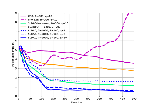
(a)

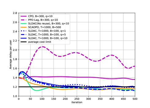
(b)

Figure 1: The number of antennas $N_{t}=8$ and the number of users $K=4$. (a) The learning curve of power consumption. (b) The learning curve of average delay per user.

V-B Constrained Linear-Quadratic Regulator

Similar to [39], we impose one constraint on the LQR, and set the state dimension $n_{\boldsymbol{s}}=15$ and action dimension $n_{\boldsymbol{a}}=4$, respectively. The cost matrices $Q_{0}$ and $R_{0}$ in (3) are semi-positive definite matrices, and the transition matrices $\boldsymbol{X}$ and $\boldsymbol{Y}$ in (4) are Gaussian matrices. The constants in the surrogate problems are $\zeta_{i}=10,\forall i$. Specially, we choose the step sizes $\alpha_{t}=\frac{1}{t^{0.6}}$, $\beta_{t}=\frac{1}{t^{0.8}}$, and $\gamma_{t}=\frac{1}{t^{0.27}}$.

In Fig. 2-(a) and Fig. 2-(b) we plot the learning curves of objective cost and constraint cost, respectively. As it can be seen from the figures, we obtain a similar behavior as in Section V-A that the proposed SLDAC with appropriately chosen $q$ provides the best performance.

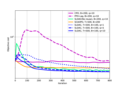
(a)

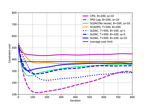
(b)

Figure 2: (a) The learning curve of objective cost. (b) The learning curve of constraint cost.

VI Conclusion

In this work, we proposed a novel SLDAC algorithm, which is the first DAC variant to solve general CMDP with guaranteed convergence. Different from the framework of classical DAC algorithms, the proposed SLDAC adopts a single-loop iteration to make the critic step and the actor step converge simultaneously to reduce the interaction cost with the environment. Considering the stochasticity and the non-convexity of both the objective function and the constraints, the SLDAC uses the CSSCA method to update the policy. Specially, we construct convex surrogate functions by reusing old observations to reduce the variance and improve the efficiency of observation. Under some technical conditions, we provide finite-time convergence rate analysis of the critic step with the Q-functions parameterized by DNNs and further prove that the SLDAC converges to a KKT point of the original problem almost surely. Simulation results show that the proposed SLDAC can achieve a better overall performance compared to baselines with much lower interaction cost.

Appendix A Technical Bounds about DNN

In this section, we show some bounds for the critic DNNs and the error introduced by the local linearization. We restate a useful lemma from recent studies of overparameterized DNNs [31, Lemma 6.4], [27, Lemma B.3], and [26, Theorem 5].

Lemma 3.

(Technical Bounds about DNN)
For any $\sigma>0$, if $\boldsymbol{\omega}\in\mathbb{B}\left(\boldsymbol{\omega}_{0},R_{\boldsymbol{\omega}}\right)$ with the neighborhood radius $R_{\boldsymbol{\omega}}$ satisfying $a_{1}d^{3/2}L^{-1}m_{Q}^{-3/4}\leq R_{\boldsymbol{\omega}}\leq a_{2}L^{-6}\bigl{(}\mathrm{log}\,m_{Q}\bigr{)}^{-3}$ and the width of neural network satisfying $m_{Q}\geq a_{3}\mathrm{max}\bigl{\{}dL^{2}\mathrm{log}\left(m_{Q}/\sigma\right),R_{\boldsymbol{\omega}}^{-4/3}L^{-8/3}\mathrm{log}\left(m_{Q}/\left(R_{\boldsymbol{\omega}}\sigma\right)\right)\bigr{\}}$, then for all $\boldsymbol{\phi}\bigl{(}\boldsymbol{s},\boldsymbol{a}\bigr{)}\in\mathbb{R}^{d}$, it holds that the difference between the $f\left(\boldsymbol{\omega}\right)$ and its local linearization $\hat{f}\left(\boldsymbol{\omega}\right)$

$$\bigl{|}f\left(\boldsymbol{\omega};\boldsymbol{s},\boldsymbol{a}\right)-\hat{f}\left(\boldsymbol{\omega};\boldsymbol{s},\boldsymbol{a}\right)\bigr{|}\leq a_{4}R_{\boldsymbol{\omega}}^{4/3}L^{4}\sqrt{m_{Q}\mathrm{log}\,m_{Q}}+a_{5}R_{\boldsymbol{\omega}}^{2}L^{5},$$

with probability at least $1-\sigma-\mathrm{exp}\bigl{\{}-a_{6}m_{Q}R_{\boldsymbol{\omega}}^{2/3}L\bigr{\}}$. Moreover, the gradient of the DNN is also bounded as $\bigl{\|}\nabla_{\boldsymbol{\omega}}f\left(\boldsymbol{\omega};\boldsymbol{s},\boldsymbol{a}\right)\bigr{\|}_{2}\leq a_{7}m_{Q}^{1/2}$ with probability at least $1-L^{2}\mathrm{exp}\bigl{\{}-a_{8}m_{Q}R_{\boldsymbol{\omega}}^{2/3}L\bigr{\}}$.

Specially, we set all critic parameters to have the same initial values, i.e. $\boldsymbol{\omega}_{0}^{i}=\boldsymbol{\bar{\omega}}_{0}^{i}=\boldsymbol{m}_{0}^{i}=\bar{\boldsymbol{m}}_{0}^{i}=\boldsymbol{\omega}_{0},\forall i$, and generate the initial parameter $\boldsymbol{\omega}_{0}$ from $\mathcal{N}\left(0,1/m_{Q}^{2}\right)$. Then, it holds that $\bigl{\|}\boldsymbol{\omega}\bigr{\|}_{2}$$\leq a_{9}m_{Q}^{1/2}$.

Appendix B Proof of Lemma 1

In this section, we present the proof of Lemma 1 in Section IV. First, to fix “learning” targets of the critic DNNs, we define two auxiliary parameters $\bigl{\{}\boldsymbol{m}^{i},\bar{\boldsymbol{m}}^{i},\forall i\bigr{\}}$, which are updated by the same rules as $\bigl{\{}\boldsymbol{\omega}^{i},\boldsymbol{\bar{\omega}}^{i},\forall i\bigr{\}}$, but uses the local linearization function $\hat{f}$ auxiliary observations $\tilde{\varepsilon}_{t}=\left\{\tilde{\boldsymbol{s}}_{t},\tilde{\boldsymbol{a}}_{t},\left\{C_{i}^{\text{'}}(\tilde{\boldsymbol{s}}_{t},\tilde{\boldsymbol{a}}_{t})\right\}_{i=0,\ldots,I},\tilde{\boldsymbol{s}}_{t+1}\right\}$ sampled by the fixed policy $\pi_{\boldsymbol{\theta}_{t}}$ from $\left(n_{t}+1\right)$-th iteration (recalling that $n_{t}=t-t^{0.6}$), which can be formulated as

$$\boldsymbol{m}_{t}^{i}=\Pi_{\Omega_{i}}\bigl{(}\boldsymbol{m}_{t-1}^{i}-\eta_{t}\boldsymbol{M}_{i}^{\boldsymbol{m}_{t}^{i}}\bigr{)},\forall i,$$ (36)

$$\bar{\boldsymbol{m}}_{t}^{i}=\bigl{(}1-\gamma_{t}\bigr{)}\bar{\boldsymbol{m}}_{t-1}^{i}+\gamma_{t}\boldsymbol{m}_{t}^{i},\forall i.$$ (37)

where recalling $\boldsymbol{\Delta}_{i}^{\boldsymbol{\omega}_{t-1}^{i}}$ defined in (14), we define the gradient term $\boldsymbol{M}_{i}^{\boldsymbol{m}_{t-1}^{i}}$ as

$$\boldsymbol{M}_{i}^{\boldsymbol{m}_{t-1}^{i}}= \Bigl{(}\hat{f}\bigl{(}\boldsymbol{m}_{t-1}^{i};\tilde{\boldsymbol{s}}_{t},\tilde{\boldsymbol{a}}_{t}\bigr{)}-\bigl{(}C_{i}^{\text{'}}(\tilde{\boldsymbol{s}}_{t},\tilde{\boldsymbol{a}}_{t})-\hat{J}_{i}^{t-1}$$ (38)

$$+\hat{f}\bigl{(}\boldsymbol{m}_{t-1}^{i};\tilde{\boldsymbol{s}}_{t+1},\tilde{\boldsymbol{a}}_{t+1}^{\prime}\bigr{)}\bigr{)}\Bigr{)}\nabla_{\boldsymbol{\omega}}f\left(\boldsymbol{m}_{0}^{i};\tilde{\boldsymbol{s}}_{t},\tilde{\boldsymbol{a}}_{t}\right),\forall i,$$

where $\tilde{\boldsymbol{a}}_{t+1}^{\prime}$ is the action chosen by current policy at the next state $\tilde{\boldsymbol{s}}_{t+1}$. Now, recalling the critic DNNs parameters in Section IV, and according to triangle inequality, we have

$$\Bigl{|}f\bigl{(}\mathbb{E}\bigl{[}\bar{\boldsymbol{\omega}}_{t}^{i}\bigr{]}\bigr{)}-\hat{Q}_{i}^{\pi_{\boldsymbol{\theta}_{t}}}\Bigl{|}$$ (39)

$$\leq \underset{\mathrm{bias}_{1}}{\underbrace{\Bigl{|}\hat{f}\bigl{(}\mathbb{E}\bigl{[}\bar{\boldsymbol{m}}_{t}^{i}\bigr{]}\bigr{)}-\hat{f}\bigl{(}\dot{\boldsymbol{\omega}}_{t}^{i}\bigr{)}\Bigl{|}}}+\underset{\mathrm{bias}_{2}}{\underbrace{\Bigl{|}\hat{f}\bigl{(}\mathbb{E}\bigl{[}\bar{\boldsymbol{\omega}}_{t}^{i}\bigr{]}\bigr{)}-\hat{f}\bigl{(}\mathbb{E}\bigl{[}\bar{\boldsymbol{m}}_{t}^{i}\bigr{]}\bigr{)}\Bigl{|}}}$$

$$+\underset{\mathrm{bias}_{3}}{\underbrace{\Bigl{|}f\bigl{(}\mathbb{E}\bigl{[}\bar{\boldsymbol{\omega}}_{t}^{i}\bigr{]}\bigr{)}-\hat{f}\bigl{(}\mathbb{E}\bigl{[}\bar{\boldsymbol{\omega}}_{t}^{i}\bigr{]}\bigr{)}\Bigl{|}}},\forall i,$$

where we denote $\mathbb{E}\left[\cdot\right]$ as the expectation taken conditional on $\boldsymbol{\omega}_{0}^{i}$ with respect to the empirical state-action distribution of $p_{t}$, which changes as policy $\pi_{\boldsymbol{\theta}_{t}}$ adjust during the process. Bias 1 characterizes the error induced by finite iterations, bias 2 presents the distance between the fixed policy update trajectory and the unfixed policy update trajectory, and bias 3 is the local linearization error. Then, in the following, we derive the three biases, respectively.

bias 1

According to the recursive operation (37), we have

$$\bar{\boldsymbol{m}}_{t}^{i}=\stackrel{{\scriptstyle[}}{{t}}^{\prime}=0]{t}{\sum}\stackrel{{\scriptstyle[}}{{j}}=t^{\prime}+1]{t}{\prod}\bigl{(}1-\gamma_{j}\bigr{)}\gamma_{t^{\prime}}\boldsymbol{m}_{t^{\prime}}^{i},\forall i,$$ (40)

Noting that $\stackrel{{\scriptstyle[}}{{t}}^{\prime}=0]{t}{\sum}\stackrel{{\scriptstyle[}}{{j}}=t^{\prime}+1]{t}{\prod}\left(1-\gamma_{j}\right)\gamma_{t^{\prime}}=1$, we can obtain the following derivation according to the Jensen’s inequality,

$$\Bigl{\|}\mathbb{E}\bigl{[}\bar{\boldsymbol{m}}_{t}^{i}\bigr{]}-\dot{\boldsymbol{\omega}}_{t}^{i}\Bigl{\|}_{2}^{2}\leq \stackrel{{\scriptstyle[}}{{t}}^{\prime}=0]{t}{\sum}\stackrel{{\scriptstyle[}}{{j}}=t^{\prime}+1]{t}{\prod}\bigl{(}1-\gamma_{j}\bigr{)}\gamma_{t^{\prime}}\Bigl{\|}\mathbb{E}\bigl{[}\boldsymbol{m}_{t^{\prime}}^{i}\bigr{]}-\dot{\boldsymbol{\omega}}_{t}^{i}\Bigl{\|}_{2}^{2}$$

$$\leq \stackrel{{\scriptstyle[}}{{t}}^{\prime}=0]{t}{\sum}\bigl{(}1-\gamma_{t}\bigr{)}^{t-t^{\prime}}\gamma_{t^{\prime}}\Bigl{\|}\mathbb{E}\bigl{[}\boldsymbol{m}_{t^{\prime}}^{i}\bigr{]}-\dot{\boldsymbol{\omega}}_{t}^{i}\Bigl{\|}_{2}^{2}$$

$$\overset{a}{\leq} \stackrel{{\scriptstyle[}}{{t}}^{\prime}=0]{n_{t}}{\sum}\bigl{(}1-\gamma_{t}\bigr{)}^{t-t^{\prime}}\Bigl{\|}\mathbb{E}\bigl{[}\boldsymbol{m}_{t^{\prime}}^{i}\bigr{]}-\dot{\boldsymbol{\omega}}_{t}^{i}\Bigl{\|}_{2}^{2}$$

$$+\frac{\gamma_{n_{t}}}{\eta_{n_{t}}}\stackrel{{\scriptstyle[}}{{t}}^{\prime}=n_{t}+1]{t}{\sum}\eta_{t^{\prime}}\Bigl{\|}\mathbb{E}\bigl{[}\boldsymbol{m}_{t^{\prime}}^{i}\bigr{]}-\dot{\boldsymbol{\omega}}_{t}^{i}\Bigl{\|}_{2}^{2}.$$ (41)

For the first term of (41)-a, since $\mathrm{max}{}_{t^{\prime}=0,\ldots,n_{t}}\Bigl{\|}\mathbb{E}\bigl{[}\boldsymbol{m}_{t^{\prime}}^{i}\bigr{]}-\dot{\boldsymbol{\omega}}_{t}^{i}\Bigl{\|}_{2}^{2}\leq R_{\boldsymbol{\omega}}^{2}=O\bigl{(}m_{Q}^{-1}\bigr{)}$, we can obtain that

$$\stackrel{{\scriptstyle[}}{{t}}^{\prime}=0]{n_{t}}{\sum}\bigl{(}1-\gamma_{t}\bigr{)}^{t-t^{\prime}}\Bigl{\|}\mathbb{E}\bigl{[}\boldsymbol{m}_{t^{\prime}}^{i}\bigr{]}-\dot{\boldsymbol{\omega}}_{t}^{i}\Bigl{\|}_{2}^{2}\leq O\bigl{(}\frac{\bigl{(}1-\gamma_{t}\bigr{)}^{t-n_{t}}}{\gamma_{t}m_{Q}}\bigr{)}.$$ (42)

Now, we derive the second term of (41)-a. Recalling the update rule of (36), we have

$$\Bigl{\|}\mathbb{E}\bigl{[}\boldsymbol{m}_{t^{\prime}+1}^{i}\bigr{]}-\dot{\boldsymbol{\omega}}_{t}^{i}\Bigr{\|}_{2}^{2} =\Bigl{\|}\Pi_{\Omega_{i}}\Bigl{(}\mathbb{E}\bigl{[}\boldsymbol{m}_{t^{\prime}}^{i}\bigr{]}-\eta_{t^{\prime}}\mathbb{E}\bigl{[}\boldsymbol{M}_{i}^{\boldsymbol{m}_{t^{\prime}}^{i}}\bigr{]}\Bigr{)}-\dot{\boldsymbol{\omega}}_{t}^{i}\Bigr{\|}_{2}^{2}$$

$$\leq-2\eta_{t^{\prime}}\Bigl{\langle}\mathbb{E}\bigl{[} \boldsymbol{M}_{i}^{\boldsymbol{m}_{t^{\prime}}^{i}}\bigr{]}-\mathbb{E}\bigl{[}\boldsymbol{M}_{i}^{\dot{\boldsymbol{\omega}}_{t}^{i}}\bigr{]},\mathbb{E}\bigl{[}\boldsymbol{m}_{t^{\prime}}^{i}\bigr{]}-\dot{\boldsymbol{\omega}}_{t}^{i}\Bigr{\rangle}$$

$$+\Bigl{\|}\mathbb{E}\bigl{[}\boldsymbol{m}_{t^{\prime}}^{i} \bigr{]}-\dot{\boldsymbol{\omega}}_{t}^{i}\Bigr{\|}_{2}^{2}+\eta_{t^{\prime}}^{2}\Bigl{\|}\mathbb{E}\bigl{[}\boldsymbol{M}_{i}^{\boldsymbol{m}_{t^{\prime}}^{i}}\bigr{]}\Bigr{\|}_{2}^{2}.$$ (43)

We first analysis the inner product term of (43). Since $\hat{f}$ is a linear function approximator of the neural network function, the gradient of $\hat{f}$ satisfies a nice property that

$$\hat{f}\left(\mathbb{E}\bigl{[}\boldsymbol{m}_{t^{\prime}}^{i}\bigr{]}\right)-\hat{f}\left(\dot{\boldsymbol{\omega}}_{t}^{i}\right)=\Bigl{\langle}\nabla_{\boldsymbol{\omega}}f\left(\boldsymbol{\omega}_{0}\right),\mathbb{E}\bigl{[}\boldsymbol{m}_{t^{\prime}}^{i}\bigr{]}-\dot{\boldsymbol{\omega}}_{t}^{i}\Bigr{\rangle},$$ (44)

and thus the inner product term can be further derived as:

$$\Bigl{\langle}\mathbb{E}\bigl{[}\boldsymbol{M}_{i}^{\boldsymbol{m}_{t^{\prime}}^{i}}\bigr{]}-\mathbb{E}\bigl{[}\boldsymbol{M}_{i}^{\dot{\boldsymbol{\omega}}_{t}^{i}}\bigr{]},\mathbb{E}\bigl{[}\boldsymbol{m}_{t^{\prime}}^{i}\bigr{]}-\dot{\boldsymbol{\omega}}_{t}^{i}\Bigr{\rangle}$$ (45)

$$= \left(\mathbb{E}\bigl{[}\boldsymbol{m}_{t^{\prime}}^{i}\bigr{]}-\dot{\boldsymbol{\omega}}_{t}^{i}\right)^{\intercal}\mathbf{A}_{i}\left(\mathbb{E}\bigl{[}\boldsymbol{m}_{t^{\prime}}^{i}\bigr{]}-\dot{\boldsymbol{\omega}}_{t}^{i}\right)$$

$$= \frac{1}{2}\left(\mathbb{E}\bigl{[}\boldsymbol{m}_{t^{\prime}}^{i}\bigr{]}-\dot{\boldsymbol{\omega}}_{t}^{i}\right)^{\intercal}\Bigl{(}\mathbf{A}_{i}+\mathbf{A}_{i}^{\intercal}\Bigr{)}\left(\mathbb{E}\bigl{[}\boldsymbol{m}_{t^{\prime}}^{i}\bigr{]}-\dot{\boldsymbol{\omega}}_{t}^{i}\right)$$

$$\geq \frac{1}{2}\lambda_{\mathrm{min}}\Bigl{(}\mathbf{A}_{i}+\mathbf{A}_{i}^{\intercal}\Bigr{)}\left\|\mathbb{E}\bigl{[}\boldsymbol{m}_{t^{\prime}}^{i}\bigr{]}-\dot{\boldsymbol{\omega}}_{t}^{i}\right\|_{2}^{2}$$

$$\overset{a}{\geq} \frac{\varsigma}{2}\left\|\mathbb{E}\bigl{[}\boldsymbol{m}_{t^{\prime}}^{i}\bigr{]}-\dot{\boldsymbol{\omega}}_{t}^{i}\right\|_{2}^{2},$$

where (45)-a follows Assumption 3-2). Then, by Lemma 2 and the fact that cost (reward) function $C_{i}^{\text{'}}$ is bounded, it’s easy to prove that

$$\Bigl{\|}\mathbb{E}\bigl{[}\boldsymbol{\Delta}_{i}^{\boldsymbol{\omega}_{t}^{i}}\bigr{]}\Bigr{\|}_{2}\leq a_{10}m_{Q}^{1/2},$$ (46)

and

$$\Bigl{\|}\mathbb{E}\bigl{[}\boldsymbol{M}_{i}^{\boldsymbol{m}_{t^{\prime}}^{i}}\bigr{]}\Bigr{\|}_{2}\leq a_{11}m_{Q}^{1/2},$$ (47)

with probability at least $1-L^{2}\mathrm{exp}\bigl{\{}-a_{8}m_{Q}R_{\boldsymbol{\omega}}^{2/3}L\bigr{\}}$. Further, by substituting (45) and (47) into (43), and rearranging the terms, we can obtain that

$$\Bigl{\|}\mathbb{E}\bigl{[}\boldsymbol{m}_{t^{\prime}}^{i}\bigr{]}-\dot{\boldsymbol{\omega}}_{t}^{i}\Bigl{\|}_{2}^{2}\leq \frac{\bigl{\|}\mathbb{E}\bigl{[}\boldsymbol{m}_{t^{\prime}}^{i}\bigr{]}-\dot{\boldsymbol{\omega}}_{t}^{i}\bigr{\|}_{2}^{2}-\bigl{\|}\mathbb{E}\bigl{[}\boldsymbol{m}_{t^{\prime}+1}^{i}\bigr{]}-\dot{\boldsymbol{\omega}}_{t}^{i}\bigr{\|}_{2}^{2}}{\eta_{t^{\prime}}\varsigma}$$

$$+\frac{a_{11}^{2}m_{Q}\eta_{t^{\prime}}}{\varsigma}.$$ (48)

Taking summation on both sides of the inequality (48), we obtain

$$\stackrel{{\scriptstyle[}}{{t}}^{\prime}=n_{t}+1]{t}{\sum}\eta_{t^{\prime}}\Bigl{\|}\mathbb{E}\bigl{[}\boldsymbol{m}_{t^{\prime}}^{i}\bigr{]}-\dot{\boldsymbol{\omega}}_{t}^{i}\Bigl{\|}_{2}^{2}$$

$$\leq \frac{\bigl{\|}\mathbb{E}\bigl{[}\boldsymbol{m}_{n_{t}+1}^{i}\bigr{]}-\dot{\boldsymbol{\omega}}_{t}^{i}\bigr{\|}_{2}^{2}}{\varsigma}+\frac{a_{11}^{2}m_{Q}\eta_{n_{t}}^{2}t^{0.6}}{\varsigma}$$

$$\leq O\bigl{(}\frac{1}{\varsigma m_{Q}}+\frac{a_{11}^{2}m_{Q}\eta_{n_{t}}^{2}t^{0.6}}{\varsigma}\bigr{)},$$ (49)

where recall that $n_{t}=t-\frac{1}{\delta_{t}}$. Finally, plugging (49) into the second term of (41)-a, we can derive that

$$\frac{\gamma_{n_{t}}}{\eta_{n_{t}}}\stackrel{{\scriptstyle[}}{{t}}^{\prime}=n_{t}+1]{t}{\sum}\eta_{t^{\prime}}\Bigl{\|}\mathbb{E}\bigl{[}\boldsymbol{m}_{t^{\prime}}^{i}\bigr{]}-\dot{\boldsymbol{\omega}}_{t}^{i}\Bigl{\|}_{2}^{2}\leq O\Bigl{(}\frac{\gamma_{n_{t}}+m_{Q}^{2}\gamma_{n_{t}}\eta_{n_{t}}^{2}t^{0.6}}{m_{Q}\eta_{n_{t}}}\Bigr{)}.$$ (50)

Combining (41), (42), and (50), we have

$$\Bigl{\|}\mathbb{E}\bigl{[}\bar{\boldsymbol{m}}_{t}^{i}\bigr{]}-\dot{\boldsymbol{\omega}}_{t}^{i}\Bigl{\|}_{2}^{2}\leq O\Bigl{(}\frac{\gamma_{n_{t}}+m_{Q}^{2}\gamma_{n_{t}}\eta_{n_{t}}^{2}t^{0.6}}{m_{Q}\eta_{n_{t}}}+\frac{\bigl{(}1-\gamma_{t}\bigr{)}^{t-n_{t}}}{m_{Q}\gamma_{t}}\Bigr{)}.$$ (51)

Finally, according to (44) and the Cauchy-Schwarz inequality, we have

$$\Bigl{|}\hat{f}\bigl{(}\mathbb{E}\bigl{[}\bar{\boldsymbol{m}}_{t}^{i}\bigr{)}-\hat{f}\bigl{(}\dot{\boldsymbol{\omega}}_{t}^{i}\bigr{)}\Bigl{|} \leq\Bigl{\|}\nabla_{\boldsymbol{\omega}}f\left(\boldsymbol{\omega}_{0}^{i}\right)\Bigr{\|}_{2}\cdot\Bigl{\|}\mathbb{E}\bigl{[}\bar{\boldsymbol{m}}_{t}^{i}\bigr{]}-\dot{\boldsymbol{\omega}}_{t}^{i}\Bigr{\|}_{2}$$

$$=O\Bigl{(}\frac{\gamma_{n_{t}}^{1/2}}{\eta_{n_{t}}^{1/2}} +m_{Q}\gamma_{n_{t}}^{1/2}\eta_{n_{t}}^{1/2}t^{0.3}+\frac{\bigl{(}1-\gamma_{t}\bigr{)}^{t/2-n_{t}/2}}{\gamma_{t}^{1/2}}\Bigr{)},$$ (52)

with probability at least $1-L^{2}\mathrm{exp}\bigl{\{}-a_{8}m_{Q}R_{\boldsymbol{\omega}}^{2/3}L\bigr{\}}$.

bias 2

Together with (15) and (37), we obtain

$$\bigl{\|}\mathbb{E}\bigl{[}\bar{\boldsymbol{m}}_{t}^{i}\bigr{]}-\mathbb{E}\bigl{[}\bar{\boldsymbol{\omega}}_{t}^{i}\bigr{]}\bigr{\|}_{2}$$ (53)

$$\leq \stackrel{{\scriptstyle[}}{{t}}^{\prime}=n_{t}+1]{t}{\sum}\stackrel{{\scriptstyle[}}{{j}}=t^{\prime}+1]{t}{\prod}\bigl{(}1-\gamma_{j}\bigr{)}\gamma_{t^{\prime}}\bigl{\|}\mathbb{E}\bigl{[}\boldsymbol{m}_{t^{\prime}}^{i}\bigr{]}-\mathbb{E}\bigl{[}\boldsymbol{\omega}_{t^{\prime}}^{i}\bigr{]}\bigr{\|}_{2}$$

$$\leq \stackrel{{\scriptstyle[}}{{t}}^{\prime}=n_{t}+1]{t}{\sum}\bigl{(}1-\gamma_{t}\bigr{)}^{t-t^{\prime}}\gamma_{t^{\prime}}e_{n_{t}}^{b}$$

$$\leq O\bigl{(}e_{n_{t}}^{b}\frac{\gamma_{n_{t}}}{\gamma_{t}}\bigr{)},\forall i,$$

where $e_{n_{t}}^{b}=\mathrm{max}_{t^{\prime}=n_{t}+1,\ldots,t}\left\{\bigl{\|}\mathbb{E}\bigl{[}\boldsymbol{m}_{t^{\prime}}^{i}\bigr{]}-\mathbb{E}\bigl{[}\boldsymbol{\omega}_{t^{\prime}}^{i}\bigr{]}\bigr{\|}_{2}\right\}$. According to Assumption 2, we have $\gamma_{n_{t}}/\gamma_{t}<\infty$, and thus $O\bigl{(}e_{n_{t}}^{b}\gamma_{n_{t}}/\gamma_{t}\bigr{)}=O\bigl{(}e_{n_{t}}^{b}\bigr{)}$.

Combining (13) and (36), we have

$$\bigl{\|}\mathbb{E}\bigl{[}\boldsymbol{m}_{t^{\prime}}^{i}\bigr{]}-\mathbb{E}\bigl{[}\boldsymbol{\omega}_{t^{\prime}}^{i}\bigr{]}\bigr{\|}_{2}$$ (54)

$$\leq \stackrel{{\scriptstyle[}}{{j}}=n_{t}+1]{t^{\prime}}{\sum}\eta_{j}\Bigl{\|}\mathbb{E}\bigl{[}\boldsymbol{\Delta}_{i}^{\boldsymbol{\omega}_{j-1}^{i}}\bigr{]}-\mathbb{E}\bigl{[}\boldsymbol{M}_{i}^{\boldsymbol{m}_{j-1}^{i}}\bigr{]}\Bigr{\|}_{2}$$

$$= \stackrel{{\scriptstyle[}}{{j}}=n_{t}+1]{t^{\prime}}{\sum}\eta_{j}\Bigl{\|}\int_{\boldsymbol{s}\in\mathcal{S}}\mathbf{P}\bigl{(}S_{j}=\mathrm{d}\boldsymbol{s}\bigr{)}\int_{\boldsymbol{a}\in\mathcal{A}}\pi_{\boldsymbol{\theta}_{j}}\bigl{(}\mathrm{d}\boldsymbol{a}\mid\boldsymbol{s}\bigr{)}\boldsymbol{\Delta}_{i}^{\boldsymbol{\omega}_{j-1}^{i}}$$

$$-\int_{\tilde{\boldsymbol{s}}\in\mathcal{S}}\mathbf{P}_{\pi_{\boldsymbol{\theta}_{t}}}\int_{\tilde{\boldsymbol{a}}\in\mathcal{A}}\pi_{\boldsymbol{\theta}_{t}}\bigl{(}\mathrm{d}\tilde{\boldsymbol{a}}\mid\tilde{\boldsymbol{s}}\bigr{)}\boldsymbol{M}_{i}^{\boldsymbol{m}_{j-1}^{i}}\Bigr{\|}_{2}$$

$$\overset{a}{\leq} m_{Q}^{1/2}\stackrel{{\scriptstyle[}}{{j}}=n_{t}+1]{t^{\prime}}{\sum}\eta_{j}O\Bigl{(}\Bigl{\|}\int_{\boldsymbol{s}\in\mathcal{S}}\mathbf{P}\bigl{(}S_{j}=\mathrm{d}\boldsymbol{s}\bigr{)}\int_{\boldsymbol{a}\in\mathcal{A}}\pi_{\boldsymbol{\theta}_{j}}\bigl{(}\mathrm{d}\boldsymbol{a}\mid\boldsymbol{s}\bigr{)}$$

$$-\int_{\tilde{\boldsymbol{s}}\in\mathcal{S}}\mathbf{P}_{\pi_{\boldsymbol{\theta}_{t}}}\int_{\boldsymbol{a}\in\mathcal{A}}\pi_{\boldsymbol{\theta}_{j}}\bigl{(}\mathrm{d}\boldsymbol{a}\mid\boldsymbol{s}\bigr{)}\Bigr{\|}_{2}+\Bigl{\|}\int_{\tilde{\boldsymbol{s}}\in\mathcal{S}}\mathbf{P}_{\pi_{\boldsymbol{\theta}_{t}}}$$

$$\int_{\boldsymbol{a}\in\mathcal{A}}\pi_{\boldsymbol{\theta}_{j}}\bigl{(}\mathrm{d}\boldsymbol{a}\mid\boldsymbol{s}\bigr{)}-\int_{\tilde{\boldsymbol{s}}\in\mathcal{S}}\mathbf{P}_{\pi_{\boldsymbol{\theta}_{t}}}\int_{\tilde{\boldsymbol{a}}\in\mathcal{A}}\pi_{\boldsymbol{\theta}_{t}}\bigl{(}\mathrm{d}\tilde{\boldsymbol{a}}\mid\tilde{\boldsymbol{s}}\bigr{)}\Bigr{\|}_{2}\Bigr{)}$$

$$\overset{b}{\leq} m_{Q}^{1/2}\stackrel{{\scriptstyle[}}{{j}}=n_{t}+1]{t^{\prime}}{\sum}\eta_{j}O\bigl{(}\bigl{\|}\mathbf{P}\bigl{(}S_{j}\in\cdot\bigr{)}-\mathbf{P}_{\pi_{\boldsymbol{\theta}_{t}}}\bigr{\|}_{TV}+\bigl{\|}\boldsymbol{\theta}_{j}-\boldsymbol{\theta}_{t}\bigr{\|}_{2}\bigr{)},$$

where the inequality (54)-a uses the bounded property of $\boldsymbol{\Delta}_{i}^{\boldsymbol{\omega}_{j-1}^{i}}$ and $\boldsymbol{M}_{i}^{\boldsymbol{m}_{j-1}^{i}}$ and follows from triangle inequality. Moreover, (54)-b comes from that the policy $\pi_{\boldsymbol{\theta}}$ follows the Lipschitz continuity over $\boldsymbol{\theta}$ . For the first term of (54)-b, we have

$$\bigl{\|}\mathbf{P}\bigl{(}S_{j}\in\cdot\bigr{)}-\mathbf{P}_{\pi_{\boldsymbol{\theta}_{t}}}\bigr{\|}_{TV}$$ (55)

$$= \bigl{\|}\mathbf{P}\bigl{(}S_{j}\in\cdot\bigr{)}-\mathbf{P}_{\pi_{\boldsymbol{\theta}_{j-\tau_{j}}}}\bigr{\|}_{TV}+\bigl{\|}\mathbf{P}_{\pi_{\boldsymbol{\theta}_{j-\tau_{j}}}}-\mathbf{P}_{\pi_{\boldsymbol{\theta}_{t}}}\bigr{\|}_{TV}$$

$$\overset{a}{\leq} \lambda\rho^{\tau_{j}}+\bigl{(}\bigl{\lceil}log_{\rho}^{\lambda^{-1}}\bigr{\rceil}+\frac{1}{1-\rho}\bigr{)}O\bigl{(}\stackrel{{\scriptstyle[}}{{k}}=j-\tau_{j}+1]{t}{\sum}\beta_{k}\bigr{)},$$

where (55)-a follows the ergodicity assumption and the theoretical result of (35) and (36) in [9], and we let $\rho^{\tau_{j}}=O\left(\frac{1}{t}\right)$. Moreover, for the second term of (54)-b, we have

$$\bigl{\|}\boldsymbol{\theta}_{j}-\boldsymbol{\theta}_{t}\bigr{\|}_{2}=O\bigl{(}\stackrel{{\scriptstyle[}}{{k}}=j+1]{t}{\sum}\beta_{k}\bigr{)}.$$ (56)

By plugging (55) and (56) into (54), we obtain

$$\bigl{\|}\mathbb{E}\bigl{[}\boldsymbol{m}_{t^{\prime}}^{i}\bigr{]}-\mathbb{E}\bigl{[}\boldsymbol{\omega}_{t^{\prime}}^{i}\bigr{]}\bigr{\|}_{2}$$ (57)

$$\leq m_{Q}^{1/2}\stackrel{{\scriptstyle[}}{{j}}=n_{t}+1]{t^{\prime}}{\sum}O\Bigl{(}\eta_{j}\lambda\rho^{\tau_{j}}+\eta_{j}\stackrel{{\scriptstyle[}}{{k}}=j-\tau_{j}+1]{t}{\sum}\beta_{k}\Bigr{)}$$

$$\leq O\Bigl{(}m_{Q}^{1/2}\eta_{n_{t}}t^{-0.4}+m_{Q}^{1/2}\eta_{n_{t}}\beta_{n_{t}}t^{1.2}\Bigr{)}\text{,}$$

Thus, we have $e_{n_{t}}^{b}\leq m_{Q}^{1/2}\eta_{n_{t}}O\bigl{(}t^{-1}\delta_{t}^{-1}+\beta_{n_{t}}\delta_{t}^{-2}\bigr{)}$, and further have

$$\bigl{\|}\mathbb{E}\bigl{[}\bar{\boldsymbol{m}}_{t}^{i}\bigr{]}-\mathbb{E}\bigl{[}\bar{\boldsymbol{\omega}}_{t}^{i}\bigr{]}\bigr{\|}_{2}\leq m_{Q}^{1/2}\eta_{n_{t}}O\bigl{(}t^{-0.4}+\beta_{n_{t}}t^{1.2}\bigr{)}.$$ (58)

Finally, according to (44) and the Cauchy-Schwarz inequality, we can obtain

$$\Bigl{|}\hat{f}\bigl{(}\mathbb{E}\bigl{[}\bar{\boldsymbol{m}}_{t}^{i}\bigr{]}\bigr{)}-\hat{f}\bigl{(}\mathbb{E}\bigl{[}\bar{\boldsymbol{\omega}}_{t}^{i}\bigr{]}\bigr{)}\Bigl{|}\leq \Bigl{\|}\nabla_{\boldsymbol{\omega}}f\left(\boldsymbol{\omega}_{0}^{i}\right)\Bigr{\|}_{2}\Bigl{\|}\mathbb{E}\bigl{[}\bar{\boldsymbol{m}}_{t}^{i}\bigr{]}-\mathbb{E}\bigl{[}\bar{\boldsymbol{\omega}}_{t}^{i}\bigr{]}\Bigr{\|}_{2}$$

$$= m_{Q}\eta_{n_{t}}O\left(t^{-0.4}+\beta_{n_{t}}t^{1.2}\right),$$ (59)

with probability at least $1-L^{2}\mathrm{exp}\bigl{\{}-a_{8}m_{Q}R_{\boldsymbol{\omega}}^{2/3}L\bigr{\}}$.

bias 3

Bias 3 characterizes how far $f$ deviates from its local linearization $\hat{f}$. By Lemma 3, if we specially set the radius $R_{\boldsymbol{\omega}}=a_{0}m_{Q}^{-1/2}$, and assume that $m_{Q}$ is sufficiently large, then it holds that

$$\mathrm{bia}_{3}\leq O\left(m_{Q}^{-1/6}\sqrt{\mathrm{log}\,m_{Q}}\right)$$ (60)

Combining (39) with (52), (59), and (60), we can obtain

$$\Bigl{|}f\bigl{(}\mathbb{E}\bigl{[}\bar{\boldsymbol{\omega}}_{t}^{i}\bigr{]}\bigr{)}-\hat{Q}_{i}^{\pi_{\boldsymbol{\theta}_{t}}}\Bigl{|}$$

$$\leq O\Bigl{(}\frac{\bigl{(}1-\gamma_{t}\bigr{)}^{t/2-n_{t}/2}}{\gamma_{t}^{1/2}}+\frac{m_{Q}\gamma_{n_{t}}^{1/2}\eta_{n_{t}}^{1/2}}{\delta_{t}^{1/2}}+m_{Q}\eta_{n_{t}}t^{-1}\delta_{t}^{-1}$$

$$+\frac{\gamma_{n_{t}}^{1/2}}{\eta_{n_{t}}^{1/2}}+m_{Q}\eta_{n_{t}}\beta_{n_{t}}\delta_{t}^{-2}+m_{Q}^{-1/6}\sqrt{\mathrm{log}\,m_{Q}}\Bigr{)},$$ (61)

with probability at least $1-L^{2}\mathrm{exp}\bigl{\{}-a_{9}m_{Q}R_{\boldsymbol{\omega}}^{2/3}L\bigr{\}}$. When the width of DNN is sufficiently large, (61) can be reduced to

$$\Bigl{|}f\bigl{(}\mathbb{E}\bigl{[}\bar{\boldsymbol{\omega}}_{t}^{i}\bigr{]}\bigr{)}-\hat{Q}_{i}^{\pi_{\boldsymbol{\theta}_{t}}}\Bigl{|}\leq O\Bigl{(}\frac{\bigl{(}1-\gamma_{t}\bigr{)}^{t/2-n_{t}/2}}{\gamma_{t}^{1/2}}+m_{Q}\gamma_{n_{t}}^{1/2}\eta_{n_{t}}^{1/2}t^{0.3}$$

$$+\frac{\gamma_{n_{t}}^{1/2}}{\eta_{n_{t}}^{1/2}}+m_{Q} \eta_{n_{t}}t^{-0.4}+m_{Q}\eta_{n_{t}}\beta_{n_{t}}t^{1.2}\Bigr{)},$$ (62)

with the probability almost $1$. This completes the proof of Lemma 1.

Appendix C Proof of Lemma 2

Our proof of Lemma 2 relies on a technical lemma [40, Lemma 1], which is restated below for completeness.

Lemma 4.

Let $(\Omega,\mathcal{G},\mathbb{P})$ denote a probability space and let $\{\mathcal{G}_{t}\}$ denote an increasing sequence of $\sigma$-field contained in $\mathcal{G}$. Let $\{z^{t}\}$, $\{w^{t}\}$ be sequences of $\mathcal{G}_{t}$-measurable random vectors satisfying the relations

$$w^{t+1}= \prod_{\mathcal{W}}(w^{t}+\alpha_{t}(\varrho^{t}-w^{t}))$$ (63)

$$\mathbb{E}[\varrho^{t}|\mathcal{G}_{t}]= z^{t}+o^{t}$$

where $\alpha_{t}\geq 0$ and the set $\mathcal{W}$ is convex and closed, $\prod_{\mathcal{W}}(\cdot)$ denotes projection on $\mathcal{W}$. Let
(a) all accumulation points of $\{w^{t}\}$ belong to $\mathcal{W}$ w.p.l.,
(b) there is a constant $C$ such that $\mathbb{E}[\|\varrho^{t}\|_{2}|\mathcal{G}_{t}]\leq C$, $\forall t\geq 0$,
(c) $\sum_{t=0}^{\infty}\mathbb{E}[(\alpha_{t})^{2}+\alpha_{t}\|o^{t}\|]\text{<}\infty$
(d) $\sum_{t=0}^{\infty}\alpha_{t}=\infty$, and (e) $\|w^{t+1}-w^{t}\|/\alpha_{t}\rightarrow 0$ w.p.l.,
Then $z^{t}-w^{t}\rightarrow 0\ w.p.1.$

By Lemma 3, we can prove the asymptotic consistency of function values (28) following the similar analysis in Appendix A-A of [9], and we omit the proof due to the space limit. Then we give the proof of (29).

We first construct an auxiliary policy gradient estimate:

$$\nabla_{\boldsymbol{\theta}}\hat{J}_{i}\left(\boldsymbol{\theta}\right)=\mathbb{E}_{\sigma_{\pi_{\boldsymbol{\theta}}}}\left[\hat{Q}_{i}^{\pi_{\boldsymbol{\theta}}}\left(\boldsymbol{s},\boldsymbol{a}\right)\nabla_{\boldsymbol{\theta}}\textrm{log}\pi_{\boldsymbol{\theta}}\left(\boldsymbol{a}\mid\boldsymbol{s}\right)\right],\forall i,$$ (64)

Note that the only difference between (20) and (64) is that we replace the exact Q-value $Q_{i}^{\pi_{\boldsymbol{\theta}_{t}}}$ with the approximate Q-functions $\hat{Q}_{i}^{\pi_{\boldsymbol{\theta}_{t}}}$. Then the asymptotic consistency of (29) can be decomposed into the following two steps:

$$\mathrm{Step}1: \underset{t\rightarrow\infty}{\mathrm{lim}}\bigl{\|}\nabla_{\boldsymbol{\theta}}\hat{J}_{i}\left(\boldsymbol{\theta}\right)-\nabla J_{i}\left(\boldsymbol{\theta}_{t}\right)\bigr{\|}_{2}=0$$ (65)

$$\mathrm{Step}2: \underset{t\rightarrow\infty}{\mathrm{lim}}\bigl{\|}\hat{\boldsymbol{g}}_{i}^{t}-\nabla_{\boldsymbol{\theta}}\hat{J}_{i}\left(\boldsymbol{\theta}\right)\bigr{\|}_{2}=0$$ (66)

Step 1

Combining (20) with (64), and together with the regularity conditions in Assumption 1, i.e., $C_{i}^{{}^{\prime}}$ and $\nabla_{\boldsymbol{\theta}}\textrm{log}\pi_{\boldsymbol{\theta}}$ are bounded, we have

$$\bigl{\|}\nabla_{\boldsymbol{\theta}}\hat{J}_{i}\left(\boldsymbol{\theta}_{t}\right)-\nabla J_{i}\left(\boldsymbol{\theta}_{t}\right)\bigr{\|}_{2}= O\bigl{(}\bigl{\|}\hat{Q}_{i}^{\pi_{\boldsymbol{\theta}}}\left(\boldsymbol{s},\boldsymbol{a}\right)-Q_{i}^{\pi_{\boldsymbol{\theta}}}\left(\boldsymbol{s},\boldsymbol{a}\right)\bigr{\|}_{2}\bigr{)}$$

$$= O\bigl{(}\bigl{\|}\hat{J}_{i}^{t}-J_{i}\left(\boldsymbol{\theta}_{t}\right)\bigr{\|}_{2}\bigr{)}$$ (67)

Recalling (28), we can complete the proof of step 1.

Step 2

Since the step size $\left\{\alpha_{t}\right\}$ follows Assumption 3, and the cost (reward) function $C_{i}(\boldsymbol{s},\boldsymbol{a})$ is bounded, it’s easy to prove that the conditions (a), (b), and (d) in Lemma 3 are satisfied. Now, we are ready to prove the technical condition (c).

Together with the definition of real gradient $\nabla J_{i}\left(\boldsymbol{\theta}_{t}\right)$ in (20), we obtain the stochastic policy gradient error between $\hat{\boldsymbol{g}}_{i}^{t}$ and $\nabla_{\boldsymbol{\theta}}\hat{J}_{i}\left(\boldsymbol{\theta}\right)$:

$$\left\|o^{t}\right\|_{2}=\bigl{\|}\hat{\boldsymbol{g}}_{i}^{t}-\nabla J_{i}\left(\boldsymbol{\theta}_{t}\right)\bigr{\|}_{2}$$ (68)

$$\overset{a}{=} \frac{1}{T_{t}}\stackrel{{\scriptstyle[}}{{l}}=1]{T_{t}}{\sum}O\bigl{(}\bigl{\|}\boldsymbol{\theta}_{t}-\boldsymbol{\theta}_{t-T_{t}+l}\bigr{\|}_{2}+\bigl{\|}\mathbf{P}\bigl{(}S_{t-T_{t}+l}\in\cdot\bigr{)}-\mathbf{P}_{\pi_{\boldsymbol{\theta}_{t}}}\bigr{\|}_{TV}$$

$$+\bigl{|}f\left(\hat{\mathbb{E}}\bigl{[}\bar{\boldsymbol{\omega}}_{t}^{i}\bigr{]};\boldsymbol{s},\boldsymbol{a}\right)-\hat{Q}_{i}^{\pi_{\boldsymbol{\theta}_{t}}}\left(\boldsymbol{s},\boldsymbol{a}\right)\bigr{|}\bigr{)},$$

where the equation (68)-a follows from similar tricks as in (54), triangle inequality, and the regularity conditions in Assumption 1, i.e., the policy $\pi_{\boldsymbol{\theta}}$ follows the Lipschitz continuity over $\boldsymbol{\theta}$, and $C_{i}^{{}^{\prime}}$, the output of DNNs and $\nabla_{\boldsymbol{\theta}}\textrm{log}\pi_{\boldsymbol{\theta}}$ are bounded. Then, plugging (55), (56) and Lemma 1 into (68), we can finally have

$$\left\|o^{t}\right\|_{2}= O\bigl{(}t^{-1}+T_{t}\beta_{t-T_{t}+1}+\frac{\bigl{(}1-\gamma_{t}\bigr{)}^{t/2-n_{t}/2}}{\gamma_{t}^{1/2}}+\frac{\gamma_{n_{t}}^{1/2}}{\eta_{n_{t}}^{1/2}}$$ (69)

$$+m_{Q}\gamma_{n_{t}}^{1/2}\eta_{n_{t}}^{1/2}t^{0.3}+m_{Q}\eta_{n_{t}}t^{-0.4}+m_{Q}\eta_{n_{t}}\beta_{n_{t}}t^{1.2}\bigr{)},$$

where we set $\rho^{\tau_{t}}=O\bigl{(}\frac{1}{t}\bigr{)}$, which means $\tau_{t}=O\bigl{(}\mathrm{log}\thinspace t\bigr{)}$ and $O\left(\textrm{log}t\right)$. According to Assumption 2, it’s easy to prove that condition (c) is held.

For the condition (e), we have

$$\bigl{\|}\nabla_{\boldsymbol{\theta}}\hat{J}_{i}\left(\boldsymbol{\theta}_{t+1}\right)-\nabla_{\boldsymbol{\theta}}\hat{J}_{i}\left(\boldsymbol{\theta}_{t}\right)\bigr{\|}_{2}$$ (70)

$$= O\bigl{(}\bigl{\|}\boldsymbol{\theta}_{t+1}-\boldsymbol{\theta}_{t}\bigr{\|}_{2}+\bigl{\|}\mathbf{P}_{\pi_{\boldsymbol{\theta}_{t+1}}}-\mathbf{P}_{\pi_{\boldsymbol{\theta}_{t}}}\bigr{\|}_{TV}\bigr{)}=O\bigl{(}\beta_{t}\bigr{)}$$

It can be seen from Assumption 2 that technical condition (e) is also satisfied. This completes the proof of step 2.

References

• [1] D. Silver, A. Huang, C. J. Maddison, A. Guez, L. Sifre, G. Van Den Driessche, J. Schrittwieser, I. Antonoglou, V. Panneershelvam, M. Lanctot et al., “Mastering the game of Go with deep neural networks and tree search,” Nature, vol. 529, no. 7587, pp. 484–489, 2016.
• [2] J. Schulman, S. Levine, P. Abbeel, M. Jordan, and P. Moritz, “Trust region policy optimization,” in ICML.   PMLR, 2015, pp. 1889–1897.
• [3] T. W. Bickmore, H. Trinh, S. Olafsson, T. K. O’Leary, R. Asadi, N. M. Rickles, and R. Cruz, “Patient and consumer safety risks when using conversational assistants for medical information: an observational study of Siri, Alexa, and Google assistant,” J Med Internet Res, vol. 20, no. 9, p. e11510, 2018.
• [4] C.-X. Wang, J. Wang, S. Hu, Z. H. Jiang, J. Tao, and F. Yan, “Key technologies in 6G terahertz wireless communication systems: A survey,” IEEE Veh. Technol. Mag., vol. 16, no. 4, pp. 27–37, 2021.
• [5] E. Altman, Constrained Markov decision processes.   CRC press, 1999, vol. 7.
• [6] P. Marbach and J. Tsitsiklis, “Simulation-based optimization of Markov reward processes: implementation issues,” in Proc. IEEE Conf. Decision Control, vol. 2, 1999, pp. 1769–1774 vol.2.
• [7] R. J. Williams, “Simple statistical gradient-following algorithms for connectionist reinforcement learning,” Reinforcement learning, pp. 5–32, 1992.
• [8] I. Grondman, L. Busoniu, G. A. D. Lopes, and R. Babuska, “A survey of actor-critic reinforcement learning: Standard and natural policy gradients,” IEEE Trans. Syst., Man, Cybern. C, Appl. Rev., vol. 42, no. 6, pp. 1291–1307, 2012.
• [9] C. Tian, A. Liu, G. Huang, and W. Luo, “Successive convex approximation based off-policy optimization for constrained reinforcement learning,” IEEE Trans. Signal Process., vol. 70, pp. 1609–1624, 2022.
• [10] R. S. Sutton and A. G. Barto, Reinforcement learning: An introduction.   MIT press, 2018.
• [11] C. Wu, S. Ohzahata, and T. Kato, “Routing in vanets: A fuzzy constraint Q-learning approach,” in Proc. IEEE Global Commun. Conf. (GLOBECOM).   IEEE, 2012, pp. 195–200.
• [12] V. R. Konda and J. N. Tsitsiklis, “Onactor-critic algorithms,” SIAM J. Control Optim., vol. 42, no. 4, pp. 1143–1166, 2003.
• [13] L. P. Kaelbling, M. L. Littman, and A. W. Moore, “Reinforcement learning: A survey,” J. Artif. Intell. Res., vol. 4, pp. 237–285, 1996.
• [14] A. Gosavi, “Reinforcement learning: A tutorial survey and recent advances,” INFORMS J. Comput., vol. 21, no. 2, pp. 178–192, 2009.
• [15] J. Achiam and D. Amodei, “Benchmarking safe exploration in deep reinforcement learning,” 2019.
• [16] J. Achiam, D. Held, A. Tamar, and P. Abbeel, “Constrained policy optimization,” in ICML.   PMLR, 2017, pp. 22–31.
• [17] Y. Zhang, Q. Vuong, and K. Ross, “First order constrained optimization in policy space,” Adv. Neural Inf. Process. Syst., vol. 33, pp. 15 338–15 349, 2020.
• [18] K. Arulkumaran, M. P. Deisenroth, M. Brundage, and A. A. Bharath, “Deep reinforcement learning: A brief survey,” IEEE Trans. Signal Process., vol. 34, no. 6, pp. 26–38, 2017.
• [19] J. Schulman, F. Wolski, P. Dhariwal, A. Radford, and O. Klimov, “Proximal policy optimization algorithms,” arXiv preprint arXiv:1707.06347, 2017.
• [20] B. Liu, Q. Cai, Z. Yang, and Z. Wang, “Neural proximal/trust region policy optimization attains globally optimal policy,” arXiv preprint arXiv:1906.10306, 2019.
• [21] A. Liu, V. K. N. Lau, and B. Kananian, “Stochastic successive convex approximation for non-convex constrained stochastic optimization,” IEEE Trans. Signal Process., vol. 67, no. 16, pp. 4189–4203, 2019.
• [22] C. B. Peel, B. M. Hochwald, and A. L. Swindlehurst, “A vector-perturbation technique for near-capacity multiantenna multiuser communication-part I: channel inversion and regularization,” IEEE Trans. Commun., vol. 53, no. 1, pp. 195–202, 2005.
• [23] B. Recht, “A tour of reinforcement learning: The view from continuous control,” Annu. Rev. Control, Robot., Auton. Syst., vol. 2, pp. 253–279, 2019.
• [24] M. Fazel, R. Ge, S. Kakade, and M. Mesbahi, “Global convergence of policy gradient methods for the linear quadratic regulator,” in ICML.   PMLR, 2018, pp. 1467–1476.
• [25] Y. Cao and Q. Gu, “Generalization error bounds of gradient descent for learning over-parameterized deep relu networks,” in Proc. AAAI Conf. Artif. Intell., vol. 34, no. 04, 2020, pp. 3349–3356.
• [26] Z. Allen-Zhu, Y. Li, and Z. Song, “A convergence theory for deep learning via over-parameterization,” in ICML.   PMLR, 2019, pp. 242–252.
• [27] Y. Cao and Q. Gu, “Generalization bounds of stochastic gradient descent for wide and deep neural networks,” Proc. Adv. Neural Inf. Process. Syst., vol. 32, 2019.
• [28] D. Zou, Y. Cao, D. Zhou, and Q. Gu, “Stochastic gradient descent optimizes over-parameterized deep Relu networks,” arXiv preprint arXiv:1811.08888, 2018.
• [29] Y. Cao and Q. Gu, “Generalization error bounds of gradient descent for learning over-parameterized deep Relu networks,” in Proc. AAAI Conf. Artif. Intell., vol. 34, no. 04, 2020, pp. 3349–3356.
• [30] R. S. Sutton and A. G. Barto, Reinforcement learning: An introduction.   MIT press, 2018.
• [31] P. Xu and Q. Gu, “A finite-time analysis of Q-learning with neural network function approximation,” in ICML.   PMLR, 2020, pp. 10 555–10 565.
• [32] S. Qiu, Z. Yang, J. Ye, and Z. Wang, “On finite-time convergence of actor-critic algorithm,” IEEE J. Sel. Areas Inf. Theory, vol. 2, no. 2, pp. 652–664, 2021.
• [33] T. Perkins and D. Precup, “A convergent form of approximate policy iteration,” Adv. Neural Inf. Process. Syst., vol. 15, 2002.
• [34] S. Zou, T. Xu, and Y. Liang, “Finite-sample analysis for sarsa with linear function approximation,” Adv. Neural Inf. Process. Syst., vol. 32, 2019.
• [35] J. N. Tsitsiklis and B. Van Roy, “Average cost temporal-difference learning,” Automatica, vol. 35, no. 11, pp. 1799–1808, 1999.
• [36] J. Fan, Z. Wang, Y. Xie, and Z. Yang, “A theoretical analysis of deep Q-learning,” in Proc. Learn. Dyn. Control.   PMLR, 2020, pp. 486–489.
• [37] S. Tosatto, M. Pirotta, C. d’Eramo, and M. Restelli, “Boosted fitted Q-iteration,” in ICML.   PMLR, 2017, pp. 3434–3443.
• [38] M. Razaviyayn, “Successive convex approximation: Analysis and applications,” Ph.D. dissertation, University of Minnesota, 2014.
• [39] M. Yu, Z. Yang, M. Kolar, and Z. Wang, “Convergent policy optimization for safe reinforcement learning,” Adv. Neural Inf. Process. Syst., vol. 32, 2019.
• [40] A. Ruszczyński, “Feasible direction methods for stochastic programming problems,” Math. Program., vol. 19, pp. 220–229, 1980.