An Optimization-based Deep Equilibrium Model for Hyperspectral Image Deconvolution with Convergence Guarantees

Abstract

In this paper, we propose a novel methodology for addressing the hyperspectral image deconvolution problem. This problem is highly ill-posed, and thus, requires proper priors (regularizers) to model the inherent spectral-spatial correlations of the HSI signals. To this end, a new optimization problem is formulated, leveraging a learnable regularizer in the form of a neural network. To tackle this problem, an effective solver is proposed using the half quadratic splitting methodology. The derived iterative solver is then expressed as a fixed-point calculation problem within the Deep Equilibrium (DEQ) framework, resulting in an interpretable architecture, with clear explainability to its parameters and convergence properties with practical benefits. The proposed model is a first attempt to handle the classical HSI degradation problem with different blurring kernels and noise levels via a single deep equilibrium model with significant computational efficiency. Extensive numerical experiments validate the superiority of the proposed methodology over other state-of-the-art methods. This superior restoration performance is achieved while requiring 99.85% less computation time as compared to existing methods.

I Introduction

In recent years, hyperspectral imaging (HSI) has emerged as a vital tool in various fields and applications, including remote sensing, medical science, and autonomous driving [1, 2]. HSI offers detailed spectral information through numerous spectral bands that is particularly useful in these areas [3]. Nonetheless, during the acquisition stage, hyperspectral images are often subject to degradation, including noise and various blurring effects, which can significantly deteriorate their performance in many HSI applications [4, 5]. Therefore, restoring hyperspectral images is a critical pre-processing step that requires efficient and effective denoising and deconvolution techniques [6].

The literature contains studies focusing on the HSI deconvolution problem, adopting diverse perspectives and assumptions to address its challenges. Despite the numerous approaches proposed so far, the problem remains open due to the inherent trade-off between high restoration accuracy and low computation time. Being a pre-processing task for various applications, it is desirable to develop methods that are both accurate and computationally efficient. However, the high-dimensional nature of hyperspectral images makes it difficult to achieve a low computational time while maintaining high restoration quality. Several well-established methodologies in this area employ filter-based methodologies, e.g., the 3D Wiener filter [7] and the Kalman filter [5], for deconvolution purposes. Additionally, other methods use Fourier and wavelet transforms to derive effective techniques for the HSI restoration problem [8]. Another direction in this field involves the incorporation of online algorithms, as seen in [9], where a sliding-block regularized Least Mean Squares (LMS) technique is employed.

Given the complexity of the HSI deconvolution problem, many methods utilize appropriate spatial and spectral priors along with other handcrafted regularizers to improve the restoration efficacy[6]. In greater detail, the method in [10] combines spatial and spectral priors in the form of optimization constraints, leading to better deconvolution results. The study in [11] proposes an optimization-based method with non-negative regularization constraints, utilizing minimum distance and maximum curvature criteria for estimating the regularization parameter. In [12], the spatial-spectral joint total variation is employed to model the 3D structure of hyperspectral images. From a spectral perspective, the works in [13, 14] introduce the dark channel prior for HSI deblurring, along with the $l0$- and $l1$-based Total Variation (TV) regularizers. In study [15], both spatial non-local self-similarity and spectral correlations investigated using low-rank tensor priors. However, developing accurate handcrafted regularization terms that capture the particular characteristics of the considered data, is not a trivial task. Furthermore, the incorporation of complex regularizers (i.e., combination of handcrafted priors) can introduce additional challenges when solving optimization problems, requiring careful parameter tuning and numerous iterations for convergence [6].

In light of this, an efficient and effective approach is proposed to encapsulate the spatial-spectral correlations typically present in hyperspectral images by building upon recent research that utilizes learnable regularization terms in the form of appropriate neural networks [16, 17, 18, 19]. These regularizers, which are learned from training data, are capable of effectively capturing more complex and unique characteristics of the considered data, as compared to the handcrafted regularizers. Subsequently, the learnable regularization terms can be employed in proper cost functions thus formulating well-justified optimization problems, leading to a method referred as “Plug-and-Play” (PnP) [20]. The majority of research efforts that fall in this category have studied 2D image processing inverse problems [21, 20]. Only, the studies in [22, 19] consider the PnP method for addressing the HSI deconvolution problem. However, it is important to note that the PnP method exhibits a significant limitation: the neural network (regularizer) is optimized without taking into account the specific inverse problem and the degraded data, hence demanding a large number of iterations and training data to achieve satisfactory performance [23].

Considering the aforementioned limitations, the proposed method focuses on formulating a new cost function for hyperspectral image deconvolution by combining a neural network, which serves as a spatial-spectral prior for the hyperspectral images, with a data consistency term. To effectively address this problem the Half-Quadratic-Splitting (HQS) method [24] is used. Contrary to plug-and-play approaches, which merely integrate the learned regularizer into the optimization problem, the derived iterative algorithm is transformed into an interpretable model-based architecture utilizing the deep unrolling [25, 26, 27, 28] and deep equilibrium [29] paradigms. In greater detail, the resulting solver is unrolled into a specific number of iterations, forming a structured neural network in which each layer represents a single iteration of the proposed algorithm. Nevertheless, the deep unrolling technique is characterized by several limitations, such as stability, and memory issues during training, necessitating the limitation of unrolling iterations to a small number [30], [21]. In view of this, we propose a more effective network-architecture using the Deep Equilibrium (DEQ) framework [29]. The DEQ approach seeks to express the network derived from the proposed iterative solver as a fixed point computation (equilibrium point), which corresponds to an architecture with an infinite number of layers. This DEQ method enables end-to-end optimization of the model, thus enhancing its adaptability to the given problem. A notable advantage of this direction is the improved interpretability of the proposed DEQ model. Its parameters directly correspond to the parameters of the optimization algorithm, which is well-understood, leading to an explainable framework with clear understanding to its operation.

From a wider viewpoint, it is interesting to note that, in realistic scenarios and settings, conventional optimization-based methods often outperform approaches that apply deep learning techniques as black-box solutions to tackle problems such as deconvolution, unmixing, or denoising in the hyperspectral domain [6, 23, 31, 32]. Optimization-based methods offer clear interpretations, leading to algorithms with a concise structure and strong generalization capabilities. However, these methods face challenges related to high computational demands and the necessity for manual hyperparameter selection [6]. On the other hand, deep learning methods, while demonstrating remarkable performance in various applications, may lack interpretability, requiring vast amounts of data to perform well and characterized by generalization issues [32]. In this work, we aim to bridge the gap between these two paradigms, by integrating optimization-based methods with novel deep learning techniques, thereby leveraging the strengths of both worlds. The derived model-based approach combines the interpretability and explainability of conventional optimization-based methods with the powerful representation capabilities of deep learning models. Consequently, more effective and efficient solutions for the hyperspectral deconvolution problem can be designed, while preserving a clear comprehension of the underlying processes and mechanisms of the physical HSI degradation model. The main contributions of this study are:

• A novel optimization problem for HSI deconvolution is proposed, involving a learnable regularizer (in the form of a deep learning network) and a data-consistency term. Based on the proposed optimization framework, an interpretable model-based method is developed for solving the HSI deconvolution problem. The approach employs the Deep Equilibrium modeling, thus expressing effectively the solution of the optimization problem as a fixed-point calculation that corresponds to an infinite-depth architecture. The proposed model is the first attempt to handle the classical HSI degradation model with different blurring kernels and noise levels via a single end-to-end deep equilibrium model with significant computation savings against the current state-of-the-art. Additionally, a deep unrolling based network is developed.

• Theoretical convergence analysis and guarantees are provided for the proposed Deep equilibrium model, with significant practical benefits. The proposed analysis provides valuable insights about the behavior of the optimization-based deep equilibrium models and how its parameters influence its convergence and stability, thus improving the model’s use and reliability in real-world applications.

• Extensive numerical results are performed in the context of the HSI deconvolution problem, demonstrating the superiority of the proposed approach against various state-of-the-art methodologies. In addition to performance restoration gains, the proposed method demands approximately $99.85\%$ less computation time as compared to the state-of-the-art approach in [19], making it ideal for real-time applications.

It should be noted that the starting point of the present work is the one in [33] where a deep equilibrium based approach for deconvolution was proposed for the first time, by the same group of authors. The main contributions and enhancements in this work, beyond those of [33], include: i) a further investigation of the proposed deep equilibrium model with emphasis on the efficient computation of the required fixed points during training and inference phases, thus reducing considerably the computational demands of the new method, ii) a rigorous convergence analysis of the deep equilibrium model leading to practical insights and benefits demonstrated via numerical results, Note that this contribution offers a clear understanding of the model’s behavior, which improves the model’s use and reliability in real-world applications. iii) development of an additional deep unrolling scheme to enable a more complete comparison with recently emerged existing approaches, iv) an extensive set of experimental evaluations, including comparisons with a broader range of state-of-the-art techniques using a wider variety of datasets.

Overall, this study establishes a novel connection between the physical modeling of the HSI blurring process, and the DEQ model. The resulting methodology comprises a highly interpretable and concise architecture, derived by utilizing prior domain knowledge for the considered problem.

II Related Work and Preliminaries

II-A Hyperspectral Deconvolution: The need for efficient solutions

As previously mentioned, the literature on HSI deconvolution mainly focuses on optimization-based methodologies that utilize spectral and spatial priors, such as those based on gradient sparsity, total variation, low-rank tensor, and non-local self-similarity to enhance the restoration performance [6, 34]. These methods offer clear interpretations and strong generalization capabilities, but they face limitations related to high computational demands and the necessity for manual hyperparameter selection.

On the other hand, deep learning techniques employed as black-box solutions [35] lack interpretability and require vast amounts of data to perform well. Furthermore, they face generalization issues [6, 32]. Recent state-of-the-art plug-and-play approaches [19, 22] attempt to merely combine the strengths of both paradigms by plugging a learned neural network prior into the iterative solutions derived from an optimization-based methodology. However, these methods still face challenges, such as a high computational burden, manual hyperparameter selection, and the necessity for large number of iterations, as the learnable prior is optimized in some pre-processing stage and independently from the optimization problem at hand. Thus, designing an efficient end-to-end model with the flexibility of the optimization based methods is actually the (open) problem that is tackled in this paper.

To fill this gap, the proposed DEQ method is able to fully integrate the merits of the optimization-based methods and the deep learning techniques. The derived method establishes a cost function for hyperspectral deblurring, integrating a neural network and a data fidelity term within the deep equilibrium paradigm. This innovative strategy offers adaptability, restoration performance, and computational efficiency while retaining a clear understanding of the underlying processes.

In this work, the focus is on non-blind HSI deconvolution, i.e., we assume that the blurring kernel is known beforehand. Non-blind HSI deconvolution is, in fact, an area of significant research activity, as highlighted in various recent studies [19, 6]. Furthermore, it should be highlighted that the proposed approach exhibits significant restoration performance even in the case where the blurring kernel is not accurately known. In more detail, as shown in the experimental results presented in Section VII-D1, our method shows notable generalization capabilities in this setting. Thus, the proposed DEQ model can be a valuable tool also in blind deconvolution scenarios where the blurring kernel can be roughly approximated using some suitable identification method.

II-B Deep equilibrium models

Deep equilibrium (DEQ) models seek to create neural networks with infinite depth by representing the whole architecture as fixed (equilibrium) point calculation [29]. Let’s consider a general K-layer deep neural network, represented by the following recursive equation

$$x^{(k+1)}=g^{(k)}_{\theta}(x^{(k)};y)\,\,\,,\,\,\,k=0,1\ldots K-1,$$ (1)

where $k$ is the layer index, $x^{(k)}$ stands for the output of the $k$-th layer, $y$ is an input shared across all layers and $g^{(k)}_{\theta}(\cdot)$ represents a nonlinear transformation corresponding to the operation of the $k$-th layer of the neural network.

Based on the DEQ modeling, it is assumed that the above non lineal transformation remains constant across all layers of the deep model, denoted as $g_{\theta}(\cdot)$. Study in [29] proposed that if we apply transformation (iteration map) $g_{\theta}(\cdot)$ an infinite number of times, the output of such model should be an equilibrium point, which satisfies the following relation:

$$x^{\star}=g_{\theta}(x^{\star};y)\ .$$ (2)

The authors of [30] have employed this methodology to tackle 2-D image restoration problems. Additionally, in our previous study in [23] we utilized the DEQ modeling to formulate a sparse coding algorithm within a deep learning architecture for representing multidimensional signals, such as hyperspectral images. However, to our knowledge, there is no published method connecting the deep equilibrium models with the classical HSI deconvolution degradation model. Motivated by this, we derive here a highly interpretable deep equilibrium architecture for tackling the HSI deconvolution problem. Different from the above studies, the proposed DEQ model stems from a novel optimization algorithm based on the HSI deconvolution degradation model involving solutions in the Fourier domain to achieve notable computational efficiency.

III Problem Formulation

Let’s denote a hyperspectral image as $\mathbf{X}\in\mathbb{R}^{M\times N\times d}$, where $M$ and $N$ represent the spatial dimensions of the image, and $d$ represents the number of spectral bands or channels. The corresponding degraded or blurred image is represented as $\mathbf{Y}\in\mathbb{R}^{M\times N\times d}$. Based on the linear degradation model [36, 22] the $i$-th spectral band of the degraded image $\boldsymbol{Y}_{i}\in{}^{M\times N}$ is given by the following relation

$$\boldsymbol{Y}_{i}=\boldsymbol{H_{i}}\star\boldsymbol{X}_{i}+\boldsymbol{W}_{i},\quad i=1,\ldots,d,$$ (3)

where $\star$ represents the convolution operator, $\boldsymbol{H_{i}}$ denotes the blurring kernel of the $i$-th spectral band and $\boldsymbol{W}_{i}$ is an additive Gaussian noise term. Considering that the blurring operator is separable across the spectral bands i.e., $\boldsymbol{H}_{i}=\boldsymbol{H}_{c}$ for $i=1\dots d$) [19, 22], the degradation model in (3) can be further simplified as

$$\boldsymbol{Y}_{i}=\boldsymbol{H}\star\boldsymbol{X}_{i}+\boldsymbol{W}_{i},\quad i=1,\ldots,d,$$ (4)

Given the blurred hyperspectral image $\boldsymbol{Y}=\{\boldsymbol{Y}_{i}\}_{i=1}^{d}$, the objective is to recover the clean image $\boldsymbol{X}$. In this study, considering ill-posed nature of the HSI deconvolution task, we propose the following regularized optimization problem:

$$\underset{\boldsymbol{X}}{\arg\min}\,\,\,\frac{1}{2}\sum_{i=1}^{d}\left\lVert\boldsymbol{Y}_{i}-\boldsymbol{H_{c}}\star\boldsymbol{X}_{i}\right\rVert_{F}^{2}+\lambda\mathcal{R}(\boldsymbol{X})\ ,$$ (5)

which consists of a data consistency term and a learnable regularizer $\mathcal{R}(\cdot)$, which seeks to capture the spatial-spectral correlations of the entire reconstructed hyperspectral image $\boldsymbol{X}=\{\boldsymbol{X}_{i}\}_{i=1}^{d}$. Moreover, $\lambda$ denotes the regularization parameter.

IV Proposed HQS solver

In order to address problem (5), the Half Quadratic Splitting (HQS) technique [4] is used, given its straightforward implementation and proven convergence capability in a variety of applications [37]. By incorporating an auxiliary variable $\boldsymbol{Z}\in{}^{M\times N\times d}$, equation (5) can be reformulated equivalently as follows:

$$\underset{\boldsymbol{X}}{\arg\min}\,\,\, \frac{1}{2}\sum_{i=1}^{d}\left\lVert\boldsymbol{Y}_{i}-\boldsymbol{H_{c}}\star\boldsymbol{X}_{i}\right\rVert_{F}^{2}+\lambda\mathcal{R}(\boldsymbol{Z})$$ (6)

$$s.t.\quad\boldsymbol{Z}-\boldsymbol{X}=0.$$

The objective of HQS is to minimize the corresponding loss function, which can be expressed as follows

$$\mathcal{L}=\frac{1}{2}\sum_{i=1}^{d}\left\lVert\boldsymbol{Y}_{i}-\boldsymbol{H_{c}}\star\boldsymbol{X}_{i}\right\rVert_{F}^{2}+\lambda\mathcal{R}(\boldsymbol{Z})+\frac{b}{2}\left\lVert\boldsymbol{Z}-\boldsymbol{X}\right\rVert_{F}^{2}$$ (7)

where b stands for a penalty parameter. Based on (7), a sequence of iterative problems can be derived i.e.,

$$\boldsymbol{X}^{(k+1)} =\underset{\boldsymbol{X}}{\arg\min}\,\,\mathcal{L}(\boldsymbol{X},\boldsymbol{Z}^{(k)})$$

$$\boldsymbol{Z}^{(k+1)} =\underset{\boldsymbol{Z}}{\arg\min}\,\,\mathcal{L}(\boldsymbol{X}^{(k+1)},\boldsymbol{Z})$$ (8)

The solutions of the above sub-problems are given by

$$\boldsymbol{X}^{(k+1)}=\underset{\boldsymbol{X}}{\arg\min}\, \frac{1}{2}\sum_{i=1}^{d}\left\lVert\boldsymbol{Y}_{i}-\boldsymbol{H_{c}}\star\boldsymbol{X}_{i}\right\rVert_{F}^{2}$$

$$\quad\quad\quad+\frac{b}{2}\left\lVert\boldsymbol{Z}^{(k)}-\boldsymbol{X}\right\rVert_{F}^{2}$$ (9a)

$$\boldsymbol{Z}^{(k+1)}=\underset{\boldsymbol{Z}}{\arg\min}\, \lambda\mathcal{R}(\boldsymbol{Z})+\frac{b}{2}\left\lVert\boldsymbol{Z}-\boldsymbol{X}^{(k+1)}\right\rVert_{F}^{2}\ .$$ (9b)

Taking into account the fact that the blurring kernel is separable over the spectral bands, and utilizing the fast Fourier transform (FFT), sub-problem (9a) can be written into a more compact and efficient form into the Fourier domain,

$$\boldsymbol{\tilde{X}}^{(k+1)}=\underset{\boldsymbol{\tilde{X}}}{\arg\min}\frac{1}{2}\left\lVert\boldsymbol{\tilde{Y}}-\boldsymbol{\tilde{H}}\odot\boldsymbol{\tilde{X}}\right\rVert_{F}^{2}+\frac{b}{2}\left\lVert\boldsymbol{\tilde{Z}}^{(k)}-\boldsymbol{\tilde{X}}\right\rVert_{F}^{2}$$ (10)

where $\tilde{\boldsymbol{Y}}=\{\mathcal{F}(\boldsymbol{Y}_{i})\}_{i=1}^{d}$, $\tilde{\boldsymbol{H}}=\{\mathcal{F}(\boldsymbol{H}_{i})\}_{i=1}^{d}$, $\tilde{\boldsymbol{X}}=\{\mathcal{F}(\boldsymbol{X}_{i})\}_{i=1}^{d}$ and $\tilde{\boldsymbol{Z}}=\{\mathcal{F}(\boldsymbol{Z}_{i})\}_{i=1}^{d}$ stand for the concatenation of the discrete 2D Fourier transforms for each spectral band of the respective spatial domain signals (i.e., $\boldsymbol{Y}_{i},\boldsymbol{H}_{i},\boldsymbol{X}_{i},\boldsymbol{Z}_{i}$). Here, $\mathcal{F}(\cdot)$ represents the 2D Fourier transform. Note that the blurring kernel $\boldsymbol{H}_{c}$ is zero-padded to the size of $\boldsymbol{X_{i}}$ before performing the discrete Fourier transform. Notably, equation (10) has a close-form solution

$$\boldsymbol{\tilde{X}}^{(k+1)}=(\boldsymbol{\tilde{H}}\odot\boldsymbol{\tilde{H}}+b\mathbb{1})^{-1}\odot(\boldsymbol{\tilde{H}}\odot\boldsymbol{\tilde{Y}}+b\boldsymbol{\tilde{Z}}^{(k)})\ .$$ (11)

Considering sub-problem (9b), it can be expressed as

$$\boldsymbol{Z}^{(k+1)}=\underset{\boldsymbol{Z}}{\arg\min}\frac{1}{2(\sqrt{\lambda/b})^{2}}\left\lVert\boldsymbol{Z}-\boldsymbol{X}^{(k+1)}\right\rVert_{F}^{2}+\mathcal{R}(\boldsymbol{Z})$$ (12)

Equation (12) corresponds to a Gaussian denoiser from a Bayesian perspective [38]. In view of this, a neural network can be employed as a denoiser, which can be trained on data to model the spatial-spectral correlations and properties of the signals under consideration. Consequently, equation (12) can be formulated as:

$$\boldsymbol{Z}^{(k+1)}=f_{\theta}(\boldsymbol{X}^{(k+1)})$$ (13)

Hence, the proposed iterative rules for the HQS are

$$\boldsymbol{Z}^{(k)} = f_{\theta}(\boldsymbol{X}^{(k)})$$ (14a)

$$\boldsymbol{\tilde{Z}}^{(k)} = \{\mathcal{F}(\boldsymbol{Z}_{i}^{(k)})\}_{i=1}^{d}$$ (14b)

$$\boldsymbol{\tilde{X}}^{(k+1)} = (\boldsymbol{\tilde{H}}\odot\boldsymbol{\tilde{H}}+b\mathbb{1})^{-1}\odot(\boldsymbol{\tilde{H}}\odot\boldsymbol{\tilde{Y}}+b\boldsymbol{\tilde{Z}}^{(k)})\quad$$ (14c)

$$\boldsymbol{X}^{(k+1)} = \{\mathcal{F}^{-1}(\tilde{\boldsymbol{X}_{i}}^{(k+1)})\}_{i=1}^{d}$$ (14d)

where $\mathcal{F}^{-1}(\cdot)$ stands for the 2D inverse Fourier transform.

To learn the weights of the neural-network $f_{\theta}(\cdot)$ we can optimize some loss function, as follows

$$\sum_{p=1}^{P}\left\lVert f_{\theta}(\boldsymbol{X}^{p}+W;\theta)-\boldsymbol{X}^{p}\right\rVert_{F}^{2}$$ (15)

In this process, we utilize a collection of $P$ paired hyperspectral images. Each pair consists of a noisy hyperspectral image, denoted as $\mathbf{X}^{(p)}+\mathbf{W}$, and its ground truth version, denoted as $\mathbf{X}^{(p)}$. Here, $\mathbf{W}$ denotes the Gaussian noise added to the original image. One approach is to use the plug-and-play framework, which involves applying the trained denoiser within the proposed update rules described in (14) and iterating until convergence is achieved. However, as the neural network optimization is independent of the blurring kernel and the blurred data, the HQS solver requires a significant number of iterations to converge and produce desirable results.

IV-A Proposed Deep Unrolling Network

Taking into account the drawbacks of the plug-and-play methodology, our aim is to develop a deep unrolling hyperspectral deconvolution network based on the proposed well-justified optimization solver (14). To accomplish this, a small number of iterations of the HQS solver (14), for instance, $K=5-10$, are unrolled to establish a highly interpretable network. Each iteration of the proposed solver corresponds to a distinct layer within this K-layer unrolling architecture. As a result, the resulting deep unrolling network yields several noteworthy advantages over conventional deep learning approaches.

In more detail, each layer consists of two steps i.e., the data consistency step (10) and the denoising step in (13). Due to the fact that the data consistency step corresponds to the degradation model, the proposed network not only takes as inputs the degraded data and the blurring kernel but also imposes a degradation constraint to the solution. It is essential to emphasize that designing such an effective multi-input system in an ad-hoc manner is not a trivial task. Figure 1 illustrates the unrolling architecture. An additional notable advantage of the proposed deep unrolling network is its capacity to train the neural network denoiser in an end-to-end manner by minimizing a loss function, such as:

$$l(\theta)=\sum_{p=1}^{P}{\left\lVert\boldsymbol{X}^{(K)}_{i}-X^{p}\right\rVert^{2}_{F}}.$$ (16)

This function encompasses pairs of generated noisy hyperspectral images (employing Gaussian noise, denoted as $\boldsymbol{W}$) and their corresponding ground truth versions, represented as $\{\boldsymbol{X}^{p}+W,\boldsymbol{X}^{p}\}_{p=1}^{P}$. Nonetheless, it is crucial to acknowledge that due to the high GPU memory resource demands, the number of unrolling iterations (layers) must be kept minimal [21], even in scenarios where the problem under consideration necessitates more iterations to achieve enhanced restoration results.

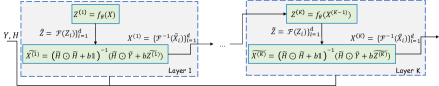
Figure 1: The proposed deep-unrolling (DU) model (Section IV-A) consisting of K layers. Each layer represents a single iteration of the iteration map in (14).

IV-B Proposed Deep Equilibrium Model

Taking into account the constraints of both plug-and-play and deep unrolling techniques, this section introduces an alternative approach. We propose an efficient network architecture that corresponds to an infinite number of layers or unrolling iterations. This architecture is inspired by Deep Equilibrium models [29], offering improved performance and flexibility. Specifically, let us represent the proposed HQS solver, consisting of the $4$ update rules as follows

$$\boldsymbol{X}^{(k+1)}=g_{\theta}(\boldsymbol{X}^{(k)};\boldsymbol{Y})\ .$$ (17)

In contrast to deep unrolling algorithm, we assume that equation (17) constructs a deep learning model with an infinite number of layers. By applying the iteration in (17) infinitely, the output will converge to a fixed point. Consequently, it will satisfy the following fixed point relation

$$\boldsymbol{X}^{\star}=g_{\theta}(\boldsymbol{X}^{\star};\boldsymbol{Y})\ .$$ (18)

As a result, using the fixed point theory, the computation of the outputs for the DEQ approach can be accelerated, as we can see in Section V-A. To train the parameters of the proposed infinite-depth architecture, which include the neural-network $f_{\theta}(\cdot)$ and the penalty parameter $b$, an end-to-end training approach can be employed. This can be accomplished by optimizing the following loss function

$$\sum_{p=1}^{P}\left\lVert g_{\theta}(\boldsymbol{X}^{\star,p},\boldsymbol{Y}^{p})-\boldsymbol{X}^{p}\right\rVert_{F}^{2},$$ (19)

where ${\boldsymbol{X}^{p},\boldsymbol{Y}^{p}}$ represent $P$ appropriate training pairs of clean hyperspectral images and their corresponding noisy and blurred images. Additionally, $g_{\theta}(\boldsymbol{X}^{\star,p};\boldsymbol{Y}^{p})=\boldsymbol{X}^{\star,p}$ is the output of the proposed DEQ model given the degraded HSI $\boldsymbol{Y}^{p}$.

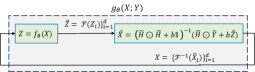
Figure 2: The proposed Deep equilibrium model, which is based on the iterative process detailed in equation 14.

V Fixed point Calculation: Forward and Backward pass

With the iteration map $g_{\theta}(\cdot,Y)$ effectively designed, two key challenges emerge. The first challenge involves computing a fixed point during the forward pass, given a noisy blurred image $Y$ and the neural network denoiser weights $\theta$. The second challenge focuses on efficiently obtaining network parameters during the training process, considering pairs of pairs of ground-truth hyperspectral images and their degraded images $\{X_{p},Y_{p}\}_{i=1}^{P}$.

To simplify notations and calculations, we examine only one pair of training data, $X$ and $Y$. Moreover, the vectorized forms of the images $Y$, and $X$, represented as $y$ and $x$ is used. This approach, without loss of generality, offers a simpler description of the problem and aids in analyzing the forward pass and training procedures of the proposed deep equilibrium model.

V-A Forward pass - Calculating fixed points

In the proposed deep equilibrium model, during both training and testing phases, a considerable number of fixed-point iterations must be executed based on the iteration map described by equation (14) to approximate the fixed point

$$x^{\star}=g_{\theta}(x^{\star},y)$$ (20)

Utilizing the following recursive scheme, the fixed-point iteration is performed

$$x^{(k+1)}=g_{\theta}(x^{(k)},y)$$ (21)

This procedure persists until convergence is reached, which occurs when $x^{(k+1)}$ and $x^{(k)}$ are adequately close together, which may introduces considerable computation burden. In view of this, we apply the Anderson acceleration technique [39], which substantially accelerates the calculation of fixed-point iterations. Specifically, the Anderson acceleration method uses $m$ previous estimate fixed points to compute the subsequent fixed point, resulting in the following solution

$$x^{(k+1)}=(1-\gamma)\sum_{i=0}^{m-1}{\beta_{i}x^{(k-i)}}+\gamma\sum_{i=0}^{m-1}{\beta_{i}g_{\theta}(x^{(k-i)},y)},$$ (22)

for $\gamma>0$. The vector $\beta\in{}^{m}$ is given as follows

$$\arg\min_{\beta}\left\lVert U\beta\right\rVert^{2}_{2},\quad s.t.\quad 1^{T}\beta=1$$ (23)

where $U=[g_{\theta}(x^{k},y)-x^{(k)},\dots,g_{\theta}(x^{k-m+1},y)-x^{(k-m+1)}]$ stands for a matrix, which contains $m$ past residuals.

V-B Backward pass - Gradient computation

During the training stage of the proposed DEQ approach, we utilize the implicit backpropagation to determine the optimal weights $\theta$. As described in [29] and [40], the objective is to train the DEQ model efficiently, avoiding the need for back-propagation across numerous iterations to reach the fixed point.

Consider the fixed point $x^{\star}=g_{\theta}(x^{\star},y)$ derived from the forward pass and a loss function $l(\cdot)$ e.g., the Mean-Squared-Error, which calculates

$$l(\theta)=\frac{1}{2}\left\lVert x^{\star}-x\right\rVert_{2}^{2}$$ (24)

The gradient of the loss with respect to the network parameters $\theta$ is given by

$$\frac{\partial l}{\partial\theta}=\frac{\partial x^{\star T}}{\partial\theta}\frac{\partial l}{\partial x^{\star}}=\left(\frac{\partial x^{\star T}}{\partial\theta}\right)\left(x^{\star}-x\right).$$ (25)

The above equation comprises two main components: the first one denotes the Jacobian of $x^{\star}$ with respect to $\theta$, while the second component is associated with the loss function gradient. However, computing the first term involves backpropagating across numerous iterations to reach a fixed point, which can be computationally expensive. To this end, we implicitly differentiate equation (20) that is $x^{\star}=g_{\theta}(x^{\star},y)$ and then proceed to utilize the multivariate chain-rule

$$\frac{\partial x^{\star}}{\partial\theta}=\frac{\partial g_{\theta}(x^{\star},y)}{\partial x^{\star}}\frac{\partial x^{\star}}{\partial\theta}+\frac{\partial g_{\theta}(x^{\star},y)}{\partial\theta}$$ (26)

By solving for $\frac{\partial x^{\star}}{\partial\theta}$ using Eq. (26), we obtain the following explicit expression for the Jacobian

$$\frac{\partial x^{\star}}{\partial\theta}=\left(I-\frac{g_{\theta}(x^{\star},y)}{\partial x^{\star}}\right)^{-1}\frac{g_{\theta}(x^{\star},y)}{\partial\theta}$$ (27)

Utilizing relation (27), we can reformulate equation (25) as

$$\frac{\partial l}{\partial\theta}=\frac{g_{\theta}(x^{\star},y)^{T}}{\partial\theta}\left(I-\frac{g_{\theta}(x^{\star},y)}{\partial x^{\star}}\right)^{-T}(x^{\star}-x).$$ (28)

As a result, we are able to compute the gradient of the loss function in a manner that is computationally efficient, eliminating the necessity for backpropagation across numerous iterations to reach a fixed point. Hence, an efficient computation of the Jacobian vector product can be performed, as demonstrated in relation (28). Following the approach presented in [40], we can compute the Jacobian vector product by defining the vector $\delta$ as

$$\delta=\left(I-\frac{g_{\theta}(x^{\star},y)}{\partial x^{\star}}\right)^{-T}(x^{\star}-x)$$

which can be reformulated as

$$\delta=\left(\frac{g_{\theta}(x^{\star},y)}{\partial x^{\star}}\right)^{T}\delta+(x^{\star}-x).$$ (29)

Interestingly, relation (29) represents a fixed point equation. Hence, given the solution of the above equation and the derived fixed-point $\delta^{\star}$, the gradient in (28) is given by

$$\frac{\partial l}{\partial\theta}=\frac{g_{\theta}(x^{\star},y)^{T}}{\partial\theta}\delta^{\star}.$$ (30)

In summary, considering the fixed point $x^{\star}$ of the iteration map $g_{\theta}(x^{\star},y)$, we adopt the following process to calculate the respective gradient:

1. Calculate the quantity $(x^{\star}-x)$ .

2. Calculate the fixed point $\delta^{\star}$, of relation (29).

3. Calculate the gradient of the loss function using equation (30).

VI Convergence Analysis

This section presents a detailed analysis of the convergence guarantees for the proposed deep equilibrium problem, based on the designed iteration map in equation (14). Recall that some operations of this iteration map (e.g., equation 14c) is expressed in the frequency domain in order to reduce the computational complexity of the iteration map. However, for simplicity, we derive an equivalent iteration map that does not involve such operations in the Fourier domain, in a mathematically equivalent manner. Therefore the final outcomes of the analysis remain valid independently of the domain in which the implementation of the recursions is performed.

Following the problem formulation of study [19, 41], the hyperspectral degradation model in (4) can be expressed as

$$y_{i}=\mathcal{H}_{i}x_{i}+w_{i}$$ (31)

where $y_{i}\in{}^{MN\times 1}$ and $x\in{}^{MN\times 1}$ are the vectorized versions of the i-th spectral bands $\boldsymbol{Y_{i}}\in{}^{M\times N}$ and $\boldsymbol{X_{i}}\in{}^{M\times N}$, respectively. $\mathcal{H}_{i}$ is a block Toeplitz matrix of size $MN\times MN$ with $M\times N$ Toeplitz blocks (see also study [19]). $\mathcal{H}_{i}$ can be rewritten as a block circulant matrix with circulant blocks, a structure denoted as circulant-block-circulant (CBC), which ensures the equivalence with the proposed designed optimization problem. Since the convolution is separable and the noise is independent over spectral bands the above degradation model is given by

$$y=\mathcal{H}x+w$$ (32)

where $\mathcal{H}$ denotes a block diagonal matrix of size $MNd\times MNd$, defined as follows

$$\begin{pmatrix}\mathcal{H}_{1}&0&\dots&0\\ 0&\ddots&\ddots&\vdots\\ \vdots&\ddots&\ddots&0\\ 0&\dots&0&\mathcal{H}_{d}\end{pmatrix}$$ (33)

Additionally, $y\in{}^{MNd\times 1}$ and $x\in{}^{MNd\times 1}$ are the vectorized versions of the images $\boldsymbol{Y}\in{}^{M\times N\times d}$ and $\boldsymbol{X}\in{}^{M\times N\times d}$, respectively.

Using the HQS method and introducing an auxiliary variable $z$, the HSI deconvolution problem is formulated as follows

$$\underset{x}{\arg\min}\,\,\, \frac{1}{2}\left\lVert y-\mathcal{H}x\right\rVert_{F}^{2}+\lambda\mathcal{R}(z)$$ (34)

$$s.t.\quad z-x=0.$$

The objective of HQS is to minimize the loss function, which can be expressed as follows

$$\mathcal{L}=\frac{1}{2}\left\lVert y-\mathcal{H}x\right\rVert_{2}^{2}+\lambda\mathcal{R}(z)+\frac{b}{2}\left\lVert z-x\right\rVert_{2}^{2}$$ (35)

The corresponding solutions of the HQS method are given by

$$z^{(k+1)} = f_{\theta}(x^{(k)})$$ (36a)

$$x^{(k+1)} = (\mathcal{H}^{T}\mathcal{H}+b\boldsymbol{I})^{-1}(\mathcal{H}^{T}y+b{z}^{(k+1)})$$ (36b)

which form the following iteration map $h_{\theta}(.,y)$ consisting of a single equation, i.e.,

$$x^{(k+1)}=(\mathcal{H}^{T}\mathcal{H}+b\boldsymbol{I})^{-1}(\mathcal{H}^{T}y+bf_{\theta}(x^{(k)}))$$ (37)

where $f_{\theta}(.)$ is the neural network that act as prior for the considered data. Note that the only difference between the above iteration map and the one in the equation 14 is that the update of the variable $x$ is performed in the spatial domain. As a result, the matrix $H$ has a significantly larger dimension, introducing considerable computational complexity compared to the iteration map that solves the update in the Fourier domain. As already mentioned in the beginning of this section, analyzing the convergence properties of the new iteration map in (37) is still valid useful for understanding the behavior of the deep equilibrium model.

VI-A Analysis

Given the iteration map in 37, i.e., $h_{\theta}(.,y):{}^{d}\rightarrow{}^{d}$, we aim to provide guarantees that the fixed point equation $x^{(k+1)}=h_{\theta}(x^{(k)},y)$ converges to a unique fixed point $x^{\star}$ as $k\rightarrow\infty$. The classical fixed-point theory [42] states that the iterative process converges to a unique fixed-point when the iteration map, denoted by $h_{\theta}(\cdot;y)$, is contractive. Note that an iteration map is contractive if there is a constant $c$ in the range $0\leq c<1$, so that the condition $||h_{\theta}(x_{1};y)-h_{\theta}(x_{2};y)||\leq c||x_{1}-x_{2}||$ is satisfied for all $x_{1},x_{2}$.

Following [43], we assume that the neural network-denoiser, represented by $f_{\theta}(\cdot)$, is $\mu$-Lipschitz continuous. This means that there exists a $\mu>0$ such that for all $x_{1},x_{2}$, the following relationship holds

$$||f_{\theta}(x_{1})-f_{\theta}(x_{2})||\leq\mu||x_{1}-x_{2}||.$$ (38)

Note that the above constraint can be easily satisfied by utilizing spectral normalization, which guarantees that the neural network will be e-Lipschitz continuous [44].

Theorem 1.

Let $f_{\theta}(\cdot)$ be a neural network denoiser that is $\mu$-Lipschitz continuous and let $L=\lambda_{\mathcal{H}^{T}\mathcal{H},min}$ be the minimum eigenvalue of $\mathcal{H}^{T}\mathcal{H}$. The iteration map $h_{\theta}(.,y)$ in (37) satisfies

$$||h_{\theta}(x_{1},y)-h_{\theta}(x_{1},y)||\leq\frac{b\,\,\mu}{(b+L)^{2}}||x_{1}-x_{2}||$$ (39)

for all $x_{1},x_{2}\in{}^{d}$. The iteration map is contractive if $\frac{b\mu}{(b+L)^{2}}<1$, in which case the proposed deep equilibrium model converges.

Proof.

Let us consider the designed iteration map $h_{\theta}(x,y)$ in equation (37). Its Jacobian with respect to $x\in\mathbb{R}^{d}$, denoted as $\partial_{x}h_{\theta}(x;y)$, is defined as follows

$$\partial_{x}h_{\theta}(x;y)=b(\mathcal{H}^{T}\mathcal{H}+b\boldsymbol{I})^{-1}\partial_{x}f_{\theta}(x)\in{}^{d\times d}$$ (40)

where $\partial_{x}f_{\theta}(x)$ denotes the Jacobian of $f_{\theta}(\cdot)$: ${}^{d}\rightarrow{}^{d}$ w.r.t x. To prove that $h_{\theta}(\cdot;y)$ is a contractive mapping, we need to show that $||\partial_{x}h_{\theta}(x;y)||<1$ holds for every $x\in{}^{d}$. Here, $||\cdot||$ represents the spectral norm. In addition, to simplify the notation, the matrix $\boldsymbol{B}=(\mathcal{H}\mathcal{H}+b\boldsymbol{I})^{-1}$ is defined. Based on equation (40), the spectral norm of the Jacobian of the iteration map is given by

$$||\partial_{x}h_{\theta}(x;y)|| =b||\boldsymbol{B}\,\partial_{x}f_{\theta}(x)||$$

$$\leq b\,\,||\boldsymbol{B}||\,\,||\partial_{x}f_{\theta}(x)||$$

$$\leq b\,\,\sigma_{B,max}\,\,\mu$$ (41)

where $\sigma_{B,max}$ stands for the maximum singular value of matrix $\boldsymbol{B}$, using the definition of the spectral norm. Note that in inequality (41), we employed the assumption in (38) that the neural network $f_{\theta}(\cdot)$ is $\mu$-Lipschitz continuous, thus the spectral norm of its Jacobian $\partial_{x}f_{\theta}(x)$ is bounded by $\mu$.

To further analyze inequality (41), we need to examine the eigenvalues of the matrix $\boldsymbol{B}$. Since $\boldsymbol{B}=(\mathcal{H}^{T}\mathcal{H}+b\boldsymbol{I})^{-1}$, it is easy to prove that the eigenvalues of $\boldsymbol{B}$ are related to the eigenvalues of the matrix $\mathcal{H}^{T}\mathcal{H}$ by the following relation

$$\lambda_{B,i}=\frac{1}{b+\lambda_{\mathcal{H}^{T}\mathcal{H},i}}$$ (42)

where $\lambda_{\mathcal{H}^{T}\mathcal{H},i}$ denotes the i-th eigenvalue of matrix $\mathcal{H}^{T}\mathcal{H}$. Since the matrix $\mathcal{H}^{T}\mathcal{H}$ is symmetric semi-positive definite and the eigenvalues of matrix $\boldsymbol{B}$, which are given by equation (42) are strictly positive, matrix $\boldsymbol{B}$ is positive definite (and symmetric). Thus, based on equation (42) its singular values are given by

$$\sigma_{B,i}=(\lambda_{B,i})^{2}=\frac{1}{(b+\lambda_{\mathcal{H}^{T}\mathcal{H},i})^{2}}$$ (43)

In view of this, the maximum singular value of matrix B is

$$\sigma_{B,max}=\frac{1}{(b+\lambda_{\mathcal{H}^{T}\mathcal{H},min})^{2}}$$ (44)

where $\lambda_{\mathcal{H}^{T}\mathcal{H},min}$ is the minimum eigenvalue of matrix $\mathcal{H}^{T}\mathcal{H}$. Based on relation 44, inequality (41) can be expressed as

$$||\partial_{x}h_{\theta}(x;y)||\leq\frac{b\mu}{(b+\lambda_{\mathcal{H}^{T}\mathcal{H},min})^{2}}$$ (45)

This proves that the iteration map $h_{\theta}(x,y)$ is $\epsilon$-Lipschitz with

$$\epsilon=\frac{b\mu}{(b+\lambda_{\mathcal{H}^{T}\mathcal{H},min})^{2}}.$$ (46)

Under the above condition, it is ensured that the proposed DEQ model will converge to a fixed point. In Section VII-D2, we provide experimental validations about the derived condition.

∎

VII Experimental part

In this section, we demonstrate the effectiveness and applicability of the proposed deep equilibrium model through extensive experiments in the context of the hyperspectral deconvolution problem. The proposed model is based on a well-justified optimization problem that utilizes a neural network for prior, allowing us to compare it with state-of-the-art works considering various optimization techniques, deep unrolling, and plug-and-play approaches. The experimental results provide strong evidence of the benefits of the proposed deep equilibrium (DEQ) model, which can be summarized as:

• Remarkably better performance compared to well-established optimization based algorithms.

• Superior performance compared to plug-and-play and deep unrolling approaches.

• Considerably less execution time compared to the state-of-the-art plug-and-play method in [19] and other optimization based approaches.

VII-A Dataset

To validate the merits of the proposed DEQ model, we used two publicly available hyperspectral image datasets, i.e., CAVE [45] dataset and the remotely sensed data Chikusei [46].

• The CAVE dataset consists of 32 hyperspectral images, each with a spatial resolution of 512 by 512 pixels 31 spectral bands in the range of 400 to 700 nm.

• The Chikusei dataset is a collection of hyperspectral images captured by a Visible and Near-Infrared imaging sensor over agricultural and urban regions in Chikusei, Ibaraki, Japan. The dataset consists of $2517\times 2335$ pixelsand covers 128 spectral channels ranging from 363 nm to 1018 nm. The spatial dimensions of the dataset were reduced by removing the black boundaries, resulting in a final image size of $2048\times 2048$ pixels.

All the hyperspectral images were normalized to the range $0-1$. In accordance with the experimental setup of the study in [22], we utilized the following blurring kernels along with Gaussian noise characterized by a standard deviation of $\sigma$ to generate the degraded images:

1. $9\times 9$ Gaussian kernel with bandwidth $\sigma_{k}=2$, and $\sigma=0.01$

2. $13\times 13$ Gaussian kernel with bandwidth $\sigma_{k}=3$, and $\sigma=0.01$

3. $9\times 9$ Gaussian kernel with bandwidth $\sigma_{k}=2$, and $\sigma=0.03$

4. Circle kernel with diameter $7$, and $\sigma=0.01$

5. Square kernel with side length of $5$, and $\sigma=0.01$

In the following experiments, we divided the CAVE dataset into two sets: a training set consisting of the first 20 images, and a test set consisting of the remaining 12 images. For the Chikusei dataset, we extracted a sub-image of size 1024 × 2048 from the top area of the image for training purposes, and then we cropped the remaining part into 32 non-overlapping sub-images of size 256 × 256 × 128 for testing.

VII-B Implementation Details

VII-B1 CNN architecture

In the proposed deep equilibrium model, a convolutional neural network $f_{\theta}(\cdot)$ with six layers was utilized to act as prior for the considered images (see, equation 14). Each convolutional layer consisted of 154 $3\times 3$ filters. Additionally, the ReLU activation function was used. To ensure that the Lipschitz constant of each layer does not exceed one, the spectral normalization [47] was applied throughout the network.

VII-B2 Hyperparameters setting

As discussed in Section IV, the CNN prior $f_{\theta}(\cdot)$ was initially pre-trained using pairs of generated noisy hyperspectral images (with varying levels of Gaussian noise) and their respective ground truth counterparts. Specifically, in a blind manner, we added i.i.d. Gaussian noise with a random standard deviation in the range of [0.2, 10] to each image. The ADAM optimizer was employed during this phase, with the training comprising $50$ epochs, a learning rate of $0.001$, and a batch size of $16$. Following pre-training, this $f_{\theta}(\cdot)$ version served as the initial point for the associated model in the proposed deep equilibrium architecture, and it was further trained during the end-to-end training process.

Regarding the DEQ model presented in Section IV-B, the Anderson acceleration technique [39] was employed to speed up fixed-point computations during the forward and backward passes in both training and testing phases, with the number of fixed-point iterations set to $15$. For the deep unrolling model discussed in Section IV-A, the number of unrolled iterations or layers was set to $K=10$. In the end-to-end training process of the DEQ and DU models, the Adam optimizer was used with a learning rate of $1e-03$ and a batch size of $6$ for $40$ epochs. Furthermore, the models were optimized for an additional $150$ epochs using a learning rate of $1e-04$.

VII-B3 Quantitative metrics

To assess the accuracy of the proposed DEQ model, we compared the reconstructed Hyperspectral Images (HSI) with their respective original images using the following metrics: (i) Peak Signal to Noise Ratio (PSNR): Higher PSNR values denote enhanced image quality, (ii) Structural Similarity Index (SSIM)[48]: Higher SSIM values indicate better preservation of spatial structure in the deconvolution image, (iii) Root Mean Square Error (RMSE): Lower RMSE values represent improved accuracy in the reconstructed image and (iv) Erreur Relative Globale Adimensionnelle de Synthese (ERGAS) [49]: A lower ERGAS value signifies better overall quality.

VII-B4 Compared Methods

As the proposed DEQ model fundamentally relies on optimization frameworks, it is compared to other optimization-based methodologies that employ either handcrafted or learnable regularizers while solving iterative algorithms. Notable examples of these methodologies include Hyper-Laplacian Priors (HLP) [41] , Spatial and Spectral Priors (SSP) [10], Weighted Low-Rank Tensor Recovery (WLRTR) [15], 3D Fractional Total Variation (3DFTV) [12], and the state-of-the-art Plug-and-Play method [19].

Additionally, utilizing the open-source HSI toolbox, called Hyde [31], we considered other three optimization based restoration approaches, i.e., the method L1HyMixDe [50], the approach Hyres [51] and the method FORDN [51]. Finally, for completeness purposes, in this study, we also examine a deep unrolling methodology presented in Section IV-A. This method serves as an intermediate solution between the plug-and-play approach [19] and the proposed DEQ model.

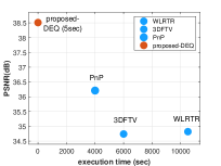
Figure 3: The execution time of our proposed DEQ model, when compared to other state-of-the-art approaches under the blurring scenario (c) in the CAVE dataset, demonstrates a significant advantage. While requiring $99.85\%$ less time than competing methods, the DEQ model still delivers superior performance, highlighting its efficiency and effectiveness in addressing hyperspectral deconvolution challenges. Note that s similar performance also exhibits the proposed DU model.

VII-C Cave and Chikusei Results

In this section, we validated the HSI deconvolution performance of the proposed DEQ model against several other approaches using the CAVE and remotely sensed Chikusei datasets. Tables II and III summarize the average results in terms of RMSE, PSNR, SSIM and ERGAS under various blurring scenarios. It is evident that the proposed DEQ model consistently outperforms the other methods in all scenarios for both datasets. Furthermore, the proposed DEQ model demonstrates superior restoration performance, particularly when dealing with high levels of noise as compared to the other methods, where their performance degrades significantly for high levels of noise.

Benefits of the concise structure of the proposed models: Moreover, an important observation can be made by examining the results shown in Table III. As previously mentioned, the Chikusei dataset consists of only one remotely sensed image. Despite the limited training data compared to the CAVE dataset, the proposed model is able to provide the best reconstruction results. The ability of the DEQ method to achieve superior performance without requiring large amounts of training data can be attributed to the fact that it has been derived from a well-justified optimization problem, thus preserving the efficient and concise nature of this approach.

Comparison with the optimization-based methods: The proposed DEQ model demonstrates a notable advantage over traditional optimization-based approaches for hyperspectral image restoration. Conventional methods depend on handcrafted regularizers to enhance restoration performance, but this strategy restricts their capacity to capture more general dependencies present in HSI images. In contrast, the DEQ model utilizes a learnable prior in the form of a CNN, allowing it to capture detailed and unique characteristics of the considered signals. This gives the DEQ model a distinct advantage over these approaches in terms of restoration performance.

Comparison with the Plug-and-play (PnP) method: Compared to the PnP approach in [19], the DEQ methodology provides notably better reconstructions results. The superior performance of the proposed DEQ model can be attributed to the end-to-end optimization of the neural-network denoiser and the penalty parameter. These components are optimized considering the quality of the reconstructed images and are specifically adapted to the examined HSI deconvolution problem. In contrast, the PnP method does not utilize an end-to-end optimization. The CNN prior is learnt separately from both the HSI degradation problem and the blurring operator.

Comparison with the deep unrolling (DU) method: Although the DU methodology (Section IV-A) provides competitive restoration results, the proposed DEQ model performed even better and that can be attributed to the following reason. Due to high GPU memory resource demands, the number of unrolling iterations in the DU method must be kept minimal, even when the problem under consideration requires more iterations for optimal restoration results. On the other hand, the DEQ model surmounts the above limitation by expressing the proposed iterative solver in (14) as a fixed point computation, thereby leading to a much more memory efficient deep architecture with an infinite number of layers.

TABLE I: Average runtime (in seconds) of the considered methods .

Method	HLP	SSP	WLRTR	3DFTV	PnP	proposed DU	proposed DEQ
time[sec]	9.7	622.5	10501.2	6044.4	4280.6	3.1	4.4

Runtime - real-time application: In terms of runtime, Figure 3 and Table I demonstrate the average execution times of the evaluated methods during the testing phase. Remarkably, the proposed DEQ method not only achieves significantly improved results but also exhibits considerably faster hyperspectral image reconstruction times. Consequently, our approach is well-suited for real-time applications, where timely and accurate processing is crucial.

TABLE II: Proposed method versus several approaches: Results under several blur scenarios on CAVE dataset.

Scenarios	Metrics	L1HyMixDe	Hyres	FORDN	HLP	SSP	WLRTR	3DFTV	PnP	proposed DU	proposed DEQ
		[50]	[52]	[52]	[41]	[10]	[15]	[12]	[19]	Section IV-A	Section IV-B
	RMSE	4.323	5.94	5.61	4.420	4.848	4.735	4.332	3.132	2.987	2.759
(a)	PSNR	35.94	35.02	34.98	36.166	35.373	35.872	36.450	39.252	39.87	40.21
	SSIM	0.9569	0.9199	0.9282	0.9167	0.9305	0.9380	0.9401	0.9493	0.9654	0.9772
	ERGAS	18.986	20.89	20.71	18.15	19.51	18.96	17.34	13.01	11.75	10.25
	RMSE	5.479	6.334	5.379	5.707	5.955	6.439	5.667	4.581	3.987	3.676
(b)	PSNR	33.14	32.57	33.21	34.034	33.541	33.084	34.116	36.305	37.64	38.050
	SSIM	0.8598	0.8223	0.8389	0.8911	0.9031	0.9025	0.9136	0.9234	0.9578	0.9565
	ERGAS	22.74	24.43	22.40	22.92	23.71	25.46	22.40	18.54	14.24	13.12
	RMSE	5.242	6.48	5.97	7.669	5.270	5.099	5.016	4.225	3.875	3.338
(c)	PSNR	34.50	32.05	33.34	30.599	34.309	34.827	34.741	36.211	37.98	38.51
	SSIM	0.8752	0.7964	0.8916	0.6406	0.8565	0.8956	0.8851	0.8708	0.9498	0.9616
	ERGAS	21.41	26.17	22.3	33.49	22.28	20.80	20.47	18.64	13.14	12.23
	RMSE	5.054	5.43	4.968	4.189	4.584	4.328	4.167	2.305	2.254	2.187
(d)	PSNR	35.12	34.22	35.171	36.549	35.862	36.68	36.80	41.65	42.01	42.55
	SSIM	0.9468	0.9214	0.9390	0.9165	0.9354	0.9450	0.9403	0.9542	0.9745	0.9801
	ERGAS	18.61	20.17	18.50	17.36	18.49	17.45	16.69	9.86	9.23	8.78
	RMSE	4.890	5.285	5.133	3.971	4.356	4.109	3.957	2.280	2.012	1.598
(e)	PSNR	35.41	34.45	34.89	36.910	36.322	37.130	37.225	41.932	44.54	45.21
	SSIM	0.9501	0.9240	0.9358	0.9195	0.9397	0.9480	0.9468	0.9475	0.9801	0.9901
	ERGAS	18.09	19.71	19.03	16.58	17.60	16.64	15.89	9.79	6.87	5.98

TABLE III: Proposed method versus several approaches: Results under several blur scenarios on Chikusei dataset.

Noise level	Metrics	L1HyMixDe	Hyres	FORDN	HLP	SSP	WLRTR	3DFTV	PnP	proposed DU	proposed DEQ
		[50]	[52]	[52]	[41]	[10]	[15]	[12]	[19]	Section IV-A	Section IV-B
	RMSE	4.27	4.41	4.321	3.233	3.050	3.138	3.207	2.560	2.398	2.228
(a)	PSNR	36.99	36.21	36.32	38.979	40.182	40.051	39.546	41.032	41.49	41.70
	SSIM	0.9116	0.8943	0.9014	0.9124	0.9334	0.9267	0.9171	0.9420	0.9587	0.9645
	ERGAS	31.72	37.89	36.87	32.25	28.13	25.29	35.37	27.87	18.97	16.33
	RMSE	5.378	5.50	5.412	3.945	3.819	4.091	4.037	3.428	3.345	3.102
(b)	PSNR	34.98	34.86	34.02	37.604	38.392	37.872	37.708	38.989	39.01	39.31
	SSIM	0.8621	0.8564	0.8612	0.8822	0.9016	0.8871	0.8819	0.9091	0.9401	0.9478
	ERGAS	39.11	40.35	39.50	35.30	32.40	31.45	39.85	30.92	29.14	28.65
	RMSE	4.444	5.30	4.69	7.094	3.506	3.777	3.662	3.413	3.012	2.805
(c)	PSNR	35.89	33.95	35.13	31.391	37.942	37.447	37.756	37.934	39.10	39.65
	SSIM	0.8799	0.8126	0.8792	0.6268	0.8839	0.8816	0.8841	0.8783	0.9498	0.9527
	ERGAS	52.24	59.33	55.52	90.14	50.26	39.95	48.15	51.38	33.54	31.65
	RMSE	4.44	4.21	4.102	3.361	2.879	2.890	3.076	2.335	2.014	1.809
(d)	PSNR	36.75	36.89	36.74	39.122	40.625	40.724	39.900	41.290	42.95	43.37
	SSIM	0.8975	0.9005	0.9012	0.9148	0.9399	0.9364	0.9228	0.9430	0.9687	0.9745
	ERGAS	36.81	34.78	34.87	32.76	27.22	23.73	34.59	32.56	17.58	16.32
	RMSE	4.025	4.014	3.901	2.990	2.688	2.691	2.913	2.148	1.987	1.678
(e)	PSNR	36.99	37.01	37.10	39.352	41.174	41.313	40.334	41.971	43.81	44.02
	SSIM	0.9193	0.9090	0.9192	0.9188	0.9456	0.9438	0.9295	0.9506	0.9665	0.9789
	ERGAS	32.00	31.02	32.15	32.68	26.19	22.46	33.74	30.62	17.84	15.78

VII-D Ablation Analysis

VII-D1 Uncertainty to blurring kernel - Generalizability

TABLE IV: PSNR results for the CAVE dataset using the DEQ model trained with blurring kernel (a) and tested with various blurring kernels, compared to the PnP method

Test Blurring Kernel	DEQ (dB)	PnP [19] (dB)
(a) 9x9 Gaussian, $\sigma_{k}$=2, $\sigma$=0.01	40.21	39.252
(b) 13x13 Gaussian, $\sigma_{k}$=3, $\sigma$=0.01	37.25	36.305
(c) 9x9 Gaussian, $\sigma_{k}$=2, $\sigma$=0.03	38.51	36.211
(d) Circle, diameter 7, $\sigma$=0.01	42.12	41.65
(e) Square, side length 5, $\sigma$=0.01	44.93	41.932

In this experiment, our objective is to evaluate the generalizability of the proposed Deep Equilibrium (DEQ) model. This is an important aspect since real-world applications often involve unknown blurring kernels, which can only be estimated, thus resulting in using noisy approximations to the actual kernel. Consequently, in many practical cases, the model may be trained with a specific blurring kernel, while during the inference phase, the actual kernel may be different. Taking this into account, we trained the DEQ model using the CAVE dataset with the blurring kernel in scenario (a), and during the testing phase, we employed several different blurring kernels, which are listed in Table IV. Additionally, we compared the proposed DEQ approach against the state-of-the-art Plug-and-Play (PnP) method.

As observed in Table IV, the DEQ model demonstrates strong generalization properties, as even in this case, it outperforms the PnP method across various blurring kernels of different sizes and types, which are distinct from the one used during training. In conclusion, the proposed deep equilibrium architecture exhibits strong generalization properties, making it a promising learning-based approach for real-world applications.

VII-D2 Convergence - Numerical validation of Theorem 1

To provide a useful intuition regarding the parameters that affect the convergence behavior of the proposed DEQ model, we conducted an experiment utilizing the Cave dataset and the blurring kernel (b). Recall that the deep equilibrium model is guaranteed to convergence to a unique fixed point if the associated iteration map is contractive. According to Theorem 1 the contractivity of the DEQ approach is ensured when the relation $\frac{b\,\,\mu}{(b+L)^{2}}<1$ is satisfied. Note that $b$ is the penalty parameter that controls the regularization term in the HQS method, $L$ denotes the minimum eigenvalue of matrix $\mathcal{H}^{T}\mathcal{H}$ and $\mu$ is the Lipschitz constant of the CNN network used for the denoising step.

For the blurring kernel in case (b), the minimum eigenvalue $L$ of matrix $\mathcal{H}^{T}\mathcal{H}$ was numerically found to have a value close to zero. Hence, the iteration map is contractive when $b>\mu$. To explore the impact of this relation and the respective parameters on the convergence on the DEQ model, we used two different values of the Lipschitz constant of the neural network $f_{\theta}(\cdot)$ i.e., $\mu=1$ and $\mu={0.075}$. Regarding the penalty parameter, we used three different values depending on the value of $\mu$, thus forming three scenarios: (i) $b<<\mu$, where $b$ is significantly smaller than $\mu$ and strongly violates the contractivity condition, (ii) $b<\mu$, where $b$ is closer to $\mu$ while still violating the contractivity condition, and (iii) $b>\mu$, thus ensuring that the developed iteration map is contractive and will converge to a fixed point. In order to quantify the convergence in all examined cases, we considered the Frobenius norm between successive fixed point estimates (i.e., between iterations $k$ and $k-1$). Figure 4 summarizes the results. It is evident from Figure 4 that a value $b>\mu$ leads to a faster and more stable convergence to a fixed point, thus validating the findings of Theorem 1.

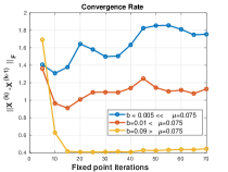
(a)

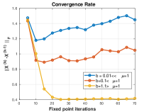
(b)

Figure 4: Numerical validation of Theorem 1 (Section VI-A). The convergence of the DEQ model is quantified by measuring the Frobenius norm between successive fixed point estimates (i.e., between fixed point estimates at iterations $k$ and $k-1$). It is demonstrated that a value $b>\mu$, as suggested by Theorem 1, leads to a faster and more stable convergence to a fixed point.

VII-D3 Influence of the number of forward iterations during inference

Plug-and-play approaches, similarly to other optimization-based methods, offer the ability to adjust the number of iterations in order to achieve satisfactory restoration results. Interestingly, the proposed deep equilibrium model also shows a similar flexibility during inference, even though it is trained end-to-end for a specific number of fixed-point iterations during the training phase. Therefore, a different number of fixed point iterations can be performed during the inference phase.

Figure 5 highlights this behavior. In particular, this figure demonstrates the performance of the DEQ and DU approaches as a function of the number of iterations performed at inference. The results show that the DEQ approach provides consistent or improved restoration performance as the number of iterations is increased, achieving a trade-off between computational efficiency and restoration performance. On the other hand, the deep unrolling method, which has been designed for a specific number of iterations, experiences a decrease in reconstruction accuracy as the number of iterations at the testing stage is increased beyond the number of iterations for which it was originally designed. The ability of the deep equilibrium model to maintain or improve its performance under varying iterations is crucial, as it highlights the model’s adaptability to different requirements. This flexibility is vital when addressing real-world scenarios where the optimal number of iterations may be unknown or subject to change based on the specific problem or application requirements.

The above finding can be attributed to a more fundamental reason. The convergence analysis of the proposed DEQ model, as detailed in Section VI, allows us to guarantee the convergence of the DEQ method. As a result, even if a specific number of fixed point iterations is performed during the training phase of the model, if this number of iterations is adequate for convergence, then the resulting model can be used for any number of iterations during inference. In fact, the iterations performed during inference constitute fixed point iterations that are guaranteed to converge to a fixed point, since the model is contractive. Overall, this observation suggests that the DEQ model, albeit a learning-based methodology, shares strong similarities with well-established optimization algorithms.

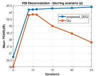
Figure 5: The comparative average performance of the proposed DEQ and the deep unrolling technique based on the number of iterations in the inference phase. The deep unrolling model was trained for K = 10 iterations at the training stage. This results in a decline in reconstruction accuracy when increasing the number of iterations at the testing stage. In contrast, the proposed deep equilibrium approach can maintain or enhance its performance over a wide range of iterations, demonstrating its adaptability and effectiveness.

VII-D4 Noise sensitivity

In this experiment, using the blurring kernel in scenario (a) and the CAVE dataset, we further examined the effectiveness of the proposed DEQ method under various noise levels. Specifically, we employed noise levels from $0.01$ to $0.05$ with an interval of $0.01$, resulting in different noise disruptions added to the input images. Table V summarizes the results. The DEQ method consistently outperforms other methods across all noise levels, demonstrating its resilience in handling various noise conditions during the HSI deconvolution problem. Additionally, although the performance of all methods generally deteriorates as the noise level increases, the DEQ method exhibits a notably smaller performance degradation, further emphasizing its efficacy.

VII-E Benefits of the Interpretability of the proposed models

As stated earlier, the deep unrolling and Deep Equilibrium models are interpretable. Their parameters directly correspond to those of the underlined optimization problem. The architecture of these models includes two interpretable components: the data consistency part and the prior denoiser part. These modules allow the effective combination of the degradation model’s structure and the a-priori knowledge of hyperspectral images. The interpretability of these models brings significant benefits. The architecture, which stems from a physical degradation process, offers a solid understanding of the network’s operations and gives insight into data processing and transformations. In addition, it provides the ability to identify cases where performance of the models may not be satisfactory, aiding in debugging and improvement. Another main advantage of these models is their ability to incorporate any denoising method, from basic designs to more elaborate deep learning architectures, without the need for model changes. This feature greatly enhances the models’ adaptability.

TABLE V: Proposed method versus several approaches: APPLIED TO THE CAVE DATASET IN THE BLURRING SCENARIO (A) WITH VARIOUS NOISE LEVELS.

Noise level	Metrics	L1HyMixDe	Hyres	FORDN	HLP	SSP	WLRTR	3DFTV	PnP	proposed DU	proposed DEQ
		[50]	[52]	[52]	[41]	[10]	[15]	[12]	[19]	Section IV-A	Section IV-B
	RMSE	4.323	5.94	5.61	4.420	4.848	4.735	4.332	3.132	2.987	2.759
$\sigma=0.01$	PSNR	35.94	35.02	34.98	36.166	35.373	35.872	36.450	39.252	39.87	40.21
	SSIM	0.9569	0.9199	0.9282	0.9167	0.9305	0.9380	0.9401	0.9493	0.9654	0.9772
	ERGAS	18.986	20.89	20.71	18.15	19.51	18.96	17.34	13.01	11.75	10.25
	RMSE	5.06	5.90	5.79	5.597	5.001	4.817	4.486	3.574	3.410	3.125
$\sigma=0.02$	PSNR	35.14	34.87	34.25	33.571	34.951	35.602	36.006	37.851	38.78	39.30
	SSIM	0.9496	0.9102	0.9094	0.8084	0.8973	0.9283	0.9301	0.9140	0.9512	0.9664
	ERGAS	19.68	21.58	21.42	23.77	20.52	19.39	17.96	15.17	12.47	11.53
	RMSE	5.242	6.48	5.97	7.669	5.270	5.099	5.016	4.225	3.875	3.338
$\sigma=0.03$	PSNR	34.50	32.05	33.34	30.599	34.309	34.827	34.741	36.211	37.98	38.51
	SSIM	0.8752	0.7964	0.8916	0.6406	0.8565	0.8956	0.8851	0.8708	0.9498	0.9616
	ERGAS	21.41	26.17	22.3	33.49	22.28	20.80	20.47	18.64	13.14	12.23
	RMSE	5.589	7.43	6.22	10.018	5.643	6.611	6.143	4.750	3.987	3.506
$\sigma=0.04$	PSNR	34.08	31.13	32.89	28.206	33.547	32.107	32.682	35.060	37.21	38.01
	SSIM	0.8650	0.7354	0.8647	0.4942	0.8155	0.7539	0.7778	0.8324	0.9347	0.9555
	ERGAS	22.00	28.77	23.46	44.43	24.66	27.42	26.05	21.37	13.51	12.90
	RMSE	6.732	8.09	6.49	12.411	6.101	9.496	7.696	5.329	4.65	3.74
$\sigma$= 0.05	PSNR	33.86	30.35	32.44	26.320	32.742	28.748	30.572	33.976	36.25	37.305
	SSIM	0.9043	0.6775	0.8402	0.3859	0.7766	0.5363	0.6462	0.7984	0.9245	0.9450
	ERGAS	23.90	31.96	24.67	55.50	27.49	40.74	33.57	24.60	15.01	13.98

VIII Conclusions

Inspired by deep equilibrium modeling, we have designed an end-to-end trainable deep network that combines the flexibility of optimization-based methods, such as generalizability and convergence properties, with the benefits of learning-based approaches, e.g. superior restoration performance and computation time efficiency. Specifically, the proposed model comprises of two interpretable modules: the data consistency step and the prior denoiser, ensuring that the network can effectively combine the structure of the degradation model and a-priori knowledge about hyperspectral images. Extensive experimental results demonstrate the flexibility, effectiveness, and generalizability of our method in the non-blind HSI deconvolution problem.

References

- [1] N. Kussul, M. Lavreniuk, S. Skakun, and A. Shelestov, “Deep learning classification of land cover and crop types using remote sensing data,” IEEE Geoscience and Remote Sensing Letters, vol. 14, no. 5, pp. 778–782, 2017.
- [2] R. Calvini, A. Ulrici, and J. M. Amigo, “Growing applications of hyperspectral and multispectral imaging,” Data Handling in Science and Technology, vol. 32, pp. 605–629, 01 2019.
- [3] A. Gkillas, D. Ampeliotis, and K. Berberidis, “Efficient coupled dictionary learning and sparse coding for noisy piecewise-smooth signals: Application to hyperspectral imaging,” in IEEE International Conference on Image Processing (ICIP), Oct. 2020.
- [4] Y. Song, D. Brie, E.-H. Djermoune, and S. Henrot, “Regularization parameter estimation for non-negative hyperspectral image deconvolution,” IEEE Transactions on Image Processing, vol. 25, no. 11, pp. 5316–5330, 2016.
- [5] S. Bongard, F. Soulez, E. Thiebaut, and E. Pecontal, “3D deconvolution of hyper-spectral astronomical data,” Monthly Notices of the Royal Astronomical Society, vol. 418, no. 1, 11 2011.
- [6] B. Rasti, Y. Chang, E. Dalsasso, L. Denis, and P. Ghamisi, “Image restoration for remote sensing: Overview and toolbox,” IEEE Geoscience and Remote Sensing Magazine, vol. 10, no. 2, pp. 201–230, 2022.
- [7] J.-M. Gaucel, M. Guillaume, and S. Bourennane, “Adaptive-3d-wiener for hyperspectral image restoration: Influence on detection strategy,” in 2006 14th European Signal Processing Conference, 2006, pp. 1–5.
- [8] R. Neelamani, H. Choi, and R. Baraniuk, “Forward: Fourier-wavelet regularized deconvolution for ill-conditioned systems,” IEEE Transactions on Signal Processing, vol. 52, no. 2, pp. 418–433, 2004.
- [9] Y. Song, E.-h. Djermoune, J. Chen, C. Richard, and D. Brie, “Online Deconvolution for Industrial Hyperspectral Imaging Systems,” SIAM Journal on Imaging Sciences, vol. 12, no. 1, pp. 54–86, 2019.
- [10] S. Henrot, C. Soussen, and D. Brie, “Fast positive deconvolution of hyperspectral images,” IEEE Transactions on Image Processing, vol. 22, no. 2, pp. 828–833, 2013.
- [11] Y. Song, D. Brie, E.-H. Djermoune, and S. Henrot, “Regularization parameter estimation for non-negative hyperspectral image deconvolution,” IEEE Transactions on Image Processing, vol. 25, no. 11, pp. 5316–5330, 2016.
- [12] L. Guo, X.-L. Zhao, X.-M. Gu, Y.-L. Zhao, Y.-B. Zheng, and T.-Z. Huang, “Three-dimensional fractional total variation regularized tensor optimized model for image deblurring,” Applied Mathematics and Computation, vol. 404, p. 126224, 2021.
- [13] S. Cao, W. Tan, K. Xing, H. He, and J. Jiang, “Dark channel inspired deblurring method for remote sensing image,” Journal of Applied Remote Sensing, vol. 12, no. 1, pp. 015 012–015 012, 2018.
- [14] H. Lim, S. Yu, K. Park, D. Seo, and J. Paik, “Texture-aware deblurring for remote sensing images using l0-based deblurring and l2-based fusion,” IEEE Journal of Selected Topics in Applied Earth Observations and Remote Sensing, vol. 13, pp. 3094–3108, 2020.
- [15] Y. Chang, L. Yan, X.-L. Zhao, H. Fang, Z. Zhang, and S. Zhong, “Weighted low-rank tensor recovery for hyperspectral image restoration,” IEEE trans on cybernetics, vol. 50, no. 11, pp. 4558–4572, 2020.
- [16] D. Gilton, G. Ongie, and R. Willett, “Learned patch-based regularization for inverse problems in imaging,” in 2019 IEEE 8th International Workshop on Computational Advances in Multi-Sensor Adaptive Processing (CAMSAP), 2019, pp. 211–215.
- [17] K. Zhang, W. Zuo, S. Gu, and L. Zhang, “Learning deep cnn denoiser prior for image restoration,” in Proceedings of the IEEE Conference on Computer Vision and Pattern Recognition (CVPR), July 2017.
- [18] G. Ongie, A. Jalal, C. A. Metzler, R. G. Baraniuk, A. G. Dimakis, and R. Willett, “Deep learning techniques for inverse problems in imaging,” IEEE J. on Selected Areas in Info Theory, vol. 1, no. 1, pp. 39–56, 2020.
- [19] X. Wang, J. Chen, and C. Richard, “Tuning-free plug-and-play hyperspectral image deconvolution with deep priors,” IEEE Transactions on Geoscience and Remote Sensing, vol. 61, pp. 1–13, 2023.
- [20] K. Zhang, Y. Li, W. Zuo, L. Zhang, L. Van Gool, and R. Timofte, “Plug-and-play image restoration with deep denoiser prior,” IEEE Transactions on Pattern Analysis and Machine Intelligence, vol. 44, no. 10, pp. 6360–6376, 2022.
- [21] V. Monga, Y. Li, and Y. C. Eldar, “Algorithm unrolling: Interpretable, efficient deep learning for signal and image processing,” IEEE Signal Processing Magazine, vol. 38, no. 2, pp. 18–44, 2021.
- [22] X. Wang, J. Chen, C. Richard, and D. Brie, “Learning spectral-spatial prior via 3ddncnn for hyperspectral image deconvolution,” in ICASSP 2020 - 2020 IEEE International Conference on Acoustics, Speech and Signal Processing (ICASSP), 2020, pp. 2403–2407.
- [23] A. Gkillas, D. Ampeliotis, and K. Berberidis, “Connections between deep equilibrium and sparse representation models with application to hyperspectral image denoising,” IEEE Transactions on Image Processing, vol. 32, pp. 1513–1528, 2023.
- [24] D. Geman and C. Yang, “Nonlinear image recovery with half-quadratic regularization,” IEEE Transactions on Image Processing, vol. 4, no. 7, pp. 932–946, 1995.
- [25] Y. Li, O. Bar-Shira, V. Monga, and Y. C. Eldar, “Deep algorithm unrolling for biomedical imaging,” arXiv:2108.06637, 2021.
- [26] Y. Ben Sahel, J. P. Bryan, B. Cleary, S. L. Farhi, and Y. C. Eldar, “Deep unrolled recovery in sparse biological imaging: Achieving fast, accurate results,” IEEE Signal Processing Magazine, vol. 39, no. 2, pp. 45–57, 2022.
- [27] Y. Yang, J. Sun, H. Li, and Z. Xu, “Admm-csnet: A deep learning approach for image compressive sensing,” IEEE Transactions on Pattern Analysis and Machine Intelligence, vol. 42, no. 3, pp. 521–538, 2020.
- [28] T. T. N. Mai, E. Y. Lam, and C. Lee, “Deep unrolled low-rank tensor completion for high dynamic range imaging,” IEEE Transactions on Image Processing, vol. 31, pp. 5774–5787, 2022.
- [29] S. Bai, J. Z. Kolter, and V. Koltun, “Deep Equilibrium Models,” in Advances in Neural Information Processing Systems, H. Wallach, H. Larochelle, A. Beygelzimer, F. d'Alché-Buc, E. Fox, and R. Garnett, Eds., vol. 32, 2019.
- [30] D. Gilton, G. Ongie, and R. Willett, “Deep equilibrium architectures for inverse problems in imaging,” IEEE Transactions on Computational Imaging, vol. 7, pp. 1123–1133, 2021.
- [31] D. Coquelin, B. Rasti, M. Götz, P. Ghamisi, R. Gloaguen, and A. Streit, “Hyde: The first open-source, python-based, gpu-accelerated hyperspectral denoising package,” 2022.
- [32] J. Chen, M. Zhao, X. Wang, C. Richard, and S. Rahardja, “Integration of physics-based and data-driven models for hyperspectral image unmixing: A summary of current methods,” IEEE Signal Processing Magazine, vol. 40, no. 2, pp. 61–74, 2023.
- [33] A. Gkillas, D. Ampeliotis, and K. Berberidis, “A highly interpretable deep equilibrium network for hyperspectral image deconvolution,” in ICASSP 2023 - 2023 IEEE International Conference on Acoustics, Speech and Signal Processing (ICASSP), 2023, pp. 1–5.
- [34] B. Rasti, P. Scheunders, P. Ghamisi, G. Licciardi, and J. Chanussot, “Noise reduction in hyperspectral imagery: Overview and application,” Remote Sensing, vol. 10, no. 3, Mar. 2018.
- [35] Y. Zhang, Y. Xiang, and L. Bai, “Generative adversarial network for deblurring of remote sensing image,” in 2018 26th International Conference on Geoinformatics, 2018, pp. 1–4.
- [36] S. Henrot, C. Soussen, and D. Brie, “Fast positive deconvolution of hyperspectral images,” IEEE Transactions on Image Processing, vol. 22, no. 2, pp. 828–833, 2013.
- [37] K. Zhang, L. Van Gool, and R. Timofte, “Deep unfolding network for image super-resolution,” in IEEE Conference on Computer Vision and Pattern Recognition, 2020, pp. 3217–3226.
- [38] C. Tian, L. Fei, W. Zheng, Y. Xu, W. Zuo, and C.-W. Lin, “Deep learning on image denoising: An overview,” Neural Networks, vol. 131, pp. 251–275, 2020.
- [39] H. F. Walker and P. Ni, “Anderson Acceleration for Fixed-Point Iterations,” http://dx.doi.org/10.1137/10078356X, vol. 49, no. 4, pp. 1715–1735, aug 2011.
- [40] “Deep Implicit Layers - Neural ODEs, Deep Equilibirum Models, and Beyond.” [Online]. Available: http://implicit-layers-tutorial.org/
- [41] D. Krishnan and R. Fergus, “Fast Image Deconvolution using Hyper-Laplacian Priors,” in Advances in Neural Information Processing Systems, Y. Bengio, D. Schuurmans, J. Lafferty, C. Williams, and A. Culotta, Eds., vol. 22. Curran Associates, Inc., 2009.
- [42] P. Agarwal, M. Jleli, and B. Samet, Banach Contraction Principle and Applications. Singapore: Springer Singapore, 2018, pp. 1–23.
- [43] E. Ryu, J. Liu, S. Wang, X. Chen, Z. Wang, and W. Yin, “Plug-and-play methods provably converge with properly trained denoisers,” in International Conference on Machine Learning. PMLR, 2019, pp. 5546–5557.
- [44] T. Miyato, T. Kataoka, M. Koyama, and Y. Yoshida, “Spectral normalization for generative adversarial networks,” in International Conference on Learning Representations, 2018. [Online]. Available: https://openreview.net/forum?id=B1QRgziT-
- [45] F. Yasuma, T. Mitsunaga, D. Iso, and S. K. Nayar, “Generalized assorted pixel camera: Postcapture control of resolution, dynamic range, and spectrum,” IEEE Transactions on Image Processing, vol. 19, no. 9, pp. 2241–2253, 2010.
- [46] N. Yokoya and A. Iwasaki, “Airborne hyperspectral data over chikusei,” Space Appl. Lab., Univ. Tokyo, Tokyo, Japan, Tech. Rep. SAL-2016-05-27, vol. 5, 2016.
- [47] T. Miyato, T. Kataoka, M. Koyama, and Y. Yoshida, “Spectral normalization for generative adversarial networks,” CoRR, vol. abs/1802.05957, 2018. [Online]. Available: http://arxiv.org/abs/1802.05957
- [48] Z. Wang, A. Bovik, H. Sheikh, and E. Simoncelli, “Image quality assessment: from error visibility to structural similarity,” IEEE Transactions on Image Processing, vol. 13, no. 4, pp. 600–612, 2004.
- [49] L. Wald, “Quality of high resolution synthesised images: Is there a simple criterion?” in Third conference” Fusion of Earth data: merging point measurements, raster maps and remotely sensed images”. SEE/URISCA, 2000, pp. 99–103.
- [50] L. Zhuang and M. K. Ng, “Hyperspectral mixed noise removal by -norm-based subspace representation,” IEEE Journal of Selected Topics in Applied Earth Observations and Remote Sensing, vol. 13, pp. 1143–1157, 2020.
- [51] B. Rasti, M. O. Ulfarsson, and P. Ghamisi, “Automatic hyperspectral image restoration using sparse and low-rank modeling,” IEEE Geoscience and Remote Sensing Letters, vol. 14, no. 12, pp. 2335–2339, 2017.
- [52] B. Rasti, J. R. Sveinsson, M. O. Ulfarsson, and J. Sigurdsson, “First order roughness penalty for hyperspectral image denoising,” in 2013 5th Workshop on Hyperspectral Image and Signal Processing: Evolution in Remote Sensing (WHISPERS), 2013, pp. 1–4.