Quantum feedback control of a two-atom network closed by a semi-infinite waveguide

Abstract

The purpose of this paper is to study the dynamics of a coherent feedback network where two two-level atoms are coupled with a semi-infinite waveguide. In this set-up, the two-level atoms can work as the photon source, and the photons can be emitted into the waveguide via the nonchiral or chiral couplings between the atom and the waveguide, according to whether the coupling strengths between the atoms and different directional propagating modes in the waveguide are identical or not. For the photon emitted by one of the two atoms, it can be reflected by the terminal mirror, or interact with the other atom, and then the photon can re-interact with the former atom. When the two atoms are both initially excited, finally there can be two-photon, one-photon or zero-photon states in the waveguide via the spontaneous emission and feedback interactions, and this is influenced by the locations of the atoms and the chirality of the coupling between the atom and the waveguide. Similarly, if only one of the two atoms is initially excited, there can be zero or one photon in the waveguide. Thus we can control the number of the photons in the waveguide and the atomic states by tuning the feedback loop length and the chiral couplings between the atom and waveguide. The photonic state in the waveguide is analyzed in the frequency domain and the spatial domain, and the transient process of photon emissions can be better understood based on the comprehensive analysis in these two domains.

1 Introduction

Feedback dynamics widely exists in quantum systems and has been explored in quantum information processing (QIP) and quantum engineering [1]. On the one hand, in measurement feedback control, the measurement results of quantum states can be used to design control signals that regulate the quantum plant [2, 3, 4]. Measurement feedback can be applied to correct error bits in quantum computation [5], squeeze light fields [6] and improve quantum metrology [7]. On the other hand, in coherent feedback control, quantum information flows in the network composed of the quantum plant and the quantum controller, without being demolished by measurements [8, 9, 10]. Coherent feedback control has found interesting applications in mechanical cooling [11], quantum error correction [12], squeezing [13], entanglement generation [14], among others.

In a quantum coherent feedback network based on waveguide quantum electrical dynamical (waveguide QED) systems, an atom can be directly coupled with the waveguide [15], or coupled with a resonant cavity and the cavity is coupled with the waveguide [16]. The atom can function as a photon source via spontaneous emission, and the emitted photons can be transmitted in the waveguide and work as the link in a quantum communication and computation network [17, 18, 19, 20]. Thus the photon can also be called the flying qubit because of its advantage of sharing quantum information and generating correlated states among standing nodes [21, 22, 23]. Single photon states are experimentally available in varied platforms such as neutral atoms [24, 25], superconducting circuits [22, 26], trapped ions [27, 28, 29], quantum dots [30, 31], and so on. Entanglement between two artificial atoms can be experimentally realized via the mediation of a single photon [32, 33]. Multi-photon states can be generated by the emission of multiple excited two-level atoms [16, 34, 35], a multi-level atom initially at the higher energy levels [36, 37] or a two-level atom which is driven repeatedly [38]. For example, in the theoretical and experimental study based on quantum dots, the two-photon state can be generated by re-exciting the quantum dot after emitting the first photon, then the quantum dot can emit two photons after two spontaneous emission processes [38].

For the feedback design based on a semi-infinite waveguide coupled with a cavity QED system [39, 40], the atom can emit photons into the cavity, and the photons in the cavity can be transmitted into the waveguide which is terminated with a perfectly reflecting mirror. The photons reflected by the mirror can further re-interact with the cavity-QED system to realize a feedback loop. The feedback dynamics can be controlled by tuning the feedback loop length and the coupling strengths among the atom, cavity and waveguide, thus the photonic state in this feedback network can be engineered. Another more efficient scheme is that atoms are directly coupled with an infinite [15, 34, 41, 42, 43, 44, 45, 46, 47, 48] or a semi-infinite [49, 46, 47, 50] waveguide. When atoms are coupled with an infinite waveguide, the feedback dynamics occurs when the photons are traveling among different atoms. For example, the photon emitted by the first atom can be absorbed and re-emitted by the second atom, then the photon in the waveguide can re-interact with the first atom, and this reflection process by the second atom can construct a feedback loop [48]. If the atoms are coupled with a semi-infinite waveguide, the terminal mirror of the waveguide can provide an additional feedback mechanism, which makes the feedback dynamics more rich. Recently, the dynamics that atoms are coupled with a semi-infinite waveguide has been analyzed for the single atom circumstance demonstrating controllable emission of single photons [46], two atoms with one exchanged excitation to create entangled states [49], the matrix product state with multi atoms [47] and the non-Markovian dynamics of giant atoms [50], in which the feedback dynamics is different according to connection topology of the giant atoms. In summary, the waveguide can be coupled with the atoms in varied formats, while the feedback dynamics with at most two excitations based on the architecture that two atoms are coupled with a semi-infinite waveguide has not yet been systematically investigated.

Depending on whether the coupling strengths between the quantum unit (e.g., an atom or a cavity) and the propagating fields in the waveguide along different directions are identical or not, the interaction between the quantum unit and the waveguide can be categorized to be chiral or nonchiral [51], and this can be fulfilled via the waveguide material design and adding external control fields [52, 53, 54]. Recently, the chiral interactions have been realized in varied experimental platforms. For example, quantum dots (QDs) coupled with a chiral photonic waveguide can induce directional emission of photons [54]; the chiral light-matter interactions have been realized with a spin chirally coupled with a nanofiber [55], and have varied applications in photon routing [56], imaging [57], optical storage [58], and so on. For atoms chirally coupled with a waveguide, the difference of the coupling strengths along the right and left directions can influence the preference direction of photon emissions in the hybrid systems such as a waveguide coupled with one atom [59, 60], the entangled two-atom network with one excitation [49, 61] and the multi-atom network coupled with an infinite waveguide with two entangled photons [41]. Take the entanglement generation between two atoms chirally coupled with a semi-infinite waveguide as an example, the chiral interactions can preserve the entanglement with a longer duration time and better robustness compared with the nonchiral coupling circumstance [49]. Furthermore, if the two atoms are both initially excited, the chirality can influence the transient process and the steady photonic states in the waveguide.

To mathematically analyze the feedback interactions between atoms and waveguide, the dynamics of the quantum system can be modeled in the frequency domain or in the spatial domain. In the frequency domain analysis, the waveguide and the atoms are coupled with a series of continuous modes, and the amplitudes of continuous photonic modes in the waveguide can be different [40, 39, 49]. In the spatial domain analysis, the photons are characterized by their spatial distributions in the waveguide, and the photons emitted by the atoms propagate in the format of wave packets [62, 59]. The atom-photon interaction in the spatial domain can be transformed from the frequency domain via the Fourier transform [48, 63, 64, 65], and the feedback of the terminal mirror can be interpreted as a boundary condition at the end of the waveguide [59]. Based on these, the evolution of the photonic state in the waveguide can be studied in terms of spatial distribution and the study can be generalized from the single-photon case to the multi-photon circumstance [66, 67, 44].

Clearly, the most desirable way to investigate the coherent feedback dynamics of atoms chirally coupled with a waveguide should be a comprehensive analysis according to both the frequency domain and spatial domain modeling. In this paper, we study a circumstance with at most two excitations based on the architecture that a semi-infinite waveguide is coupled with two two-level atoms as shown in Fig. 1. In this set-up, the evolution of the quantum states is simultaneously influenced by the feedback interactions between two atoms as in Ref. [15], the feedback dynamics induced by the mirror as in Ref. [68, 59], and the chiral interactions between the two atoms and the semi-infinite waveguide as in Ref. [49]. As a result, the photonic states in this system can be controlled by engineering the distance between two atoms, the atom locations away from the terminal mirror of the semi-infinite waveguide and the chiral coupling strengths between atoms and the waveguide. The purpose of this paper is to analyze the dynamics of this coherent feedback network in both the frequency and spatial domains, then we can engineer this coherent feedback network to generate interesting physical properties such as controllable photon source, photon memory and entangled states mediated with photons.

The rest of the paper is organized as follows. Section 2 analyzes in the frequency domain the feedback interactions when the semi-infinite waveguide is coupled with two isolated excited two-level atoms, especially how the chiral couplings and delays caused by the locations of atoms influence the performance of the feedback network. Section 3 presents the analysis in the spatial domain and clarifies that how the single photon wave packet propagates in the two-atom network mediated by a waveguide. Section 4 concludes this paper.

Notation. The reduced Planck constant $\hbar$, velocity of the light field $c$ and the group velocity for the propagating photon wave packets $v_{g}$ are samely set to be $1$ in this paper.

2 Mathematical model for two atoms coupled with a waveguide in the frequency domain

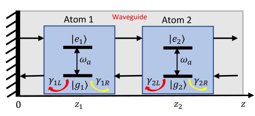
Figure 1: The control scheme of two atoms in the semi-infinite waveguide.

As shown in Fig.1, two atoms (or atomlike objects) with the same resonant frequency $\omega_{a}$ are coupled to a semi-infinite waveguide. The distance between the atoms is $L=z_{2}-z_{1}$, where $z_{j}$ is the location of the $j$th atom, $j=1,2$. The coupling strength between the $j$th atom with the left-propagating field in the waveguide is $\gamma_{jL}$, and that with the right propagating field is $\gamma_{jR}$, where $\gamma_{jL}$ and $\gamma_{jR}$ are real constant numbers. For the atom at $z_{1}$, the emitted field in the left-propagating direction can be reflected by the mirror at $z=0$ and then propagates along the right direction to re-interact with the atom. The emitted field in the right-propagating direction excites the atom at $z_{2}$. For the atom at $z_{2}$, the emitted filed in the left-propagating direction can excite the atom at $z_{1}$, while the emitted filed in the right-propagating direction leaves the system.

The following assumption is used in the frequency domain analysis.

Assumption 1.

Initially, both of the two atoms are in their excited states, the waveguide is empty, and there are no external drives.

The interaction Hamiltonian between the atoms and the waveguide in the interaction picture can be written as [47, 69, 70, 46, 49]

$$H_{I} =i\sum_{j=1,2}\int\mathrm{d}k\;\left[\left(d^{{\dagger}}_{k}\sigma_{j}^{-}\gamma_{jR}e^{-i\omega z_{j}/c}e^{-i\frac{\Phi}{2}}e^{i(\omega-\omega_{a})t}-d^{{\dagger}}_{k}\sigma_{j}^{-}\gamma_{jL}e^{i\omega z_{j}/c}e^{i\frac{\Phi}{2}}e^{i(\omega-\omega_{a})t}\right)-\mathrm{H.c.}\right],$$ (1)

where $\sigma_{j}^{-}=|g_{j}\rangle\langle e_{j}|$ and $\sigma_{j}^{+}=|e_{j}\rangle\langle g_{j}|$ are the lowering and raising operators of the $j$th atom, $c$ is the velocity of the field in the waveguide, $k$ is the continuous mode with frequency $\omega=ck$, $d_{k}$($d_{k}^{{\dagger}}$) are the annihilation(creation) operators of the propagating waveguide modes, and $\Phi$ is the reflection-induced phase delay by the mirror which is experimentally small [59], $\mathrm{H.c.}$ denotes Hermitian conjugate. The continuous coupled modes between the atoms and the waveguide are integrated within $[0,+\infty)$ in this paper. Denote $\tilde{z}_{j}=z_{j}+\frac{\Phi}{2k}$. Then the interaction Hamiltonian $H_{I}$ in Eq. (1) can be re-written as

$$H_{I} =i\sum_{j=1,2}\int\mathrm{d}k\;\left[\left(d^{{\dagger}}_{k}\sigma_{j}^{-}\gamma_{jR}e^{-i\omega\tilde{z}_{j}/c}e^{i(\omega-\omega_{a})t}-d^{{\dagger}}_{k}\sigma_{j}^{-}\gamma_{jL}e^{i\omega\tilde{z}_{j}/c}e^{i(\omega-\omega_{a})t}\right)-\mathrm{H.c.}\right].$$ (2)

That is, the phase shift $\Phi$ can be ignored under the global translation of the atoms’ positions. Still using $z_{j}$ instead of $\tilde{z}_{j}$ for simplicity, the interaction Hamiltonian in the interaction picture can be further simplified as

$$H_{I}=\sum_{j=1,2}\int\mathrm{d}k\;\left[g_{kjt}(k,t,z)d^{{\dagger}}_{k}\sigma_{j}^{-}+g_{kjt}^{*}(k,t,z)d_{k}\sigma_{j}^{+}\right],$$ (3)

where

$$g_{kjt}(k,t,z) \triangleq i(\gamma_{jR}e^{-i\omega z_{j}/c}-\gamma_{jL}e^{i\omega z_{j}/c})e^{i(\omega-\omega_{a})t}.$$ (4)

When the couplings between the atoms and the waveguide are nonchiral, namely $\gamma_{jR}=\gamma_{jL}\equiv\gamma_{j}$, ($j=1,2$), the coupling strength in Eq. (4) reduce to $g_{kjt}=2\gamma_{j}\sin(kz_{j})e^{i(\omega-\omega_{a})t}$.

The Hamiltonian of the coherent feedback network in the interaction picture reads

$$H =\sum_{j=1,2}\omega_{a}\sigma_{j}^{+}\sigma_{j}^{-}+\int\mathrm{d}k\;\omega_{k}d^{{\dagger}}_{k}d_{k}+\sum_{j=1,2}\int\mathrm{d}k\;\left[g_{kjt}(k,t,z)d^{{\dagger}}_{k}\sigma_{j}^{-}+g_{kjt}^{*}(k,t,z)d_{k}\sigma_{j}^{+}\right],$$ (5)

where the first component represents the atomic Hamiltonian, the second component represents the fields in the waveguide, and the last term is the interaction Hamiltonian $H_{I}$ in Eq. (3), respectively.

According to Assumption 1, the whole system has two excitations, hence the state of coherent feedback network can be represented as

$$|\Psi(t)\rangle= c_{ee}(t)|e_{1},e_{2},\{0\}\rangle+\int c_{egk}(t,k)|e_{1},g_{2},\{k\}\rangle\mathrm{d}k+\int c_{gek}(t,k)|g_{1},e_{2},\{k\}\rangle\mathrm{d}k$$ (6)

$$+\int c_{kk}(k_{1},k_{2},t)|g_{1},g_{2},\{k_{1}\}\{k_{2}\}\rangle\mathrm{d}k_{1}\mathrm{d}k_{2},$$

where $|e_{1},e_{2},\{0\}\rangle$ means that both atoms are in the excited state and there are no photons in the waveguide, $|e_{1},g_{2},\{k\}\rangle$ indicates that the first atom is in the excited state, the second atom is in the ground state, and there is one photon in the waveguide, $|g_{1},e_{2},\{k\}\rangle$ means that the first atom is in the ground stat, the second atom is in the excited state and there is on one photon in the waveguide, $|g_{1},g_{2},\{k_{1}\}\{k_{2}\}\rangle$ represents that both of the two atoms are in the ground state and there are two photons in the waveguide. $c_{ee}(t)$, $c_{egk}(t,k)$, $c_{gek}(t,k)$, and $c_{kk}(k_{1},k_{2},t)$ are the probability amplitudes, respectively.

Solving the Schrödinger equation

$$\frac{\partial}{\partial t}|\Psi(t)\rangle=-iH|\Psi(t)\rangle$$

with the Hamiltonian in Eq. (5) and the ansatz in Eq. (6) yields a system of integro-differential equations for the amplitudes, which is

$$\dot{c}_{ee}(t)=-i\int c_{egk}(t,k)g_{k2t}^{*}(k,t,z_{2})\mathrm{d}k-i\int c_{gek}(t,k)g_{k1t}^{*}(k,t,z_{1})\mathrm{d}k,$$ (7a)

$$\dot{c}_{egk}(t,k)=-ic_{ee}(t)g_{k2t}(k,t,z_{2})-i\int c_{kk}(k,k_{1},t)g_{k1t}^{*}(k_{1},t,z_{1})\mathrm{d}k_{1},$$ (7b)

$$\dot{c}_{gek}(t,k)=-ic_{ee}(t)g_{k1t}(k,t,z_{1})-i\int c_{kk}(k,k_{1},t)g_{k2t}^{*}(k_{1},t,z_{2})\mathrm{d}k_{1},$$ (7c)

$$\dot{c}_{kk}(k_{1},k_{2},t)=-ic_{egk}(t,k_{1})g_{k1t}(k_{2},t,z_{1})-ic_{egk}(t,k_{2})g_{k1t}(k_{1},t,z_{1})$$

$$~{}~{}~{}~{}~{}~{}~{}~{}~{}~{}~{}~{}~{}~{}~{}~{}~{}~{}~{}-ic_{gek}(t,k_{1})g_{k2t}(k_{2},t,z_{2})-ic_{gek}(t,k_{2})g_{k2t}(k_{1},t,z_{2}).$$ (7d)

The physical interpretation of Eq. (7) is as follows. Eq. (7a) means that if one of the two atoms is in the excited state while the other is in the ground state, then both of two atoms can be in the excited state after absorbing one photon from the waveguide. Inversely, the first part of the right-hand side of Eq. (7b) and Eq. (7c) indicates that when the two atoms are in the excited state, one atom can emit one photon into the waveguide and decay to the ground stat; the latter part of Eq. (7b) and Eq. (7c) describes that one atom can absorb one photon from the waveguide when both of the two atoms are in the ground state. Eq. (7d) means that when only one of the two atoms is in the excited state, the excited atom can emit a photon into the waveguide, then both of the two atoms are in the ground state and there are two photons in the waveguide.

According to the calculations in Appendix A, Eq. (7a) can be rewritten as:

$$\dot{c}_{ee}(t)=-\frac{\gamma_{1R}^{2}+\gamma_{1L}^{2}+\gamma_{2R}^{2}+\gamma_{2L}^{2}}{2}c_{ee}(t)+\gamma_{1L}\gamma_{1R}c_{ee}(t-\frac{2z_{1}}{c})e^{i\omega_{a}\frac{2z_{1}}{c}}+\gamma_{2L}\gamma_{2R}c_{ee}(t-\frac{2z_{2}}{c})e^{i\omega_{a}\frac{2z_{2}}{c}},$$ (8)

which is influenced by the round trip delay between the atoms and the terminal mirror as $\tau_{j}=\frac{2z_{j}}{c}$, ($j=1,2$). Eq. (7b) can be rewritten as:

$$\dot{c}_{egk}(t,k)= -\frac{\gamma_{1R}^{2}+\gamma_{1L}^{2}}{2}c_{egk}(t,k)-ic_{ee}(t)g_{k2t}(k,t,z_{2})+\gamma_{1L}\gamma_{1R}c_{egk}(t-\frac{2z_{1}}{c},k)e^{i\omega_{a}\frac{2z_{1}}{c}}$$ (9)

$$+\gamma_{1R}\gamma_{2L}c_{gek}(t-\frac{z_{1}+z_{2}}{c},k)e^{i\omega_{a}\frac{z_{1}+z_{2}}{c}}-\gamma_{1L}\gamma_{2L}c_{gek}(t-\frac{z_{2}-z_{1}}{c},k)e^{i\omega_{a}\frac{z_{2}-z_{1}}{c}},$$

where $\frac{2z_{1}}{c}$ represents the round trip delay between the first atom and the mirror, $\frac{z_{1}+z_{2}}{c}$ represents the delay from the second atom at $z_{2}$ to the first atom at $z_{1}$ after the field being reflected by the mirror, and $\frac{z_{2}-z_{1}}{c}$ represents the delay directly from the second atom at $z_{2}$ to the first atom at $z_{1}$. Finally, Eq. (7c) can be rewritten as:

$$\dot{c}_{gek}(t,k)= -\frac{\gamma_{2R}^{2}+\gamma_{2L}^{2}}{2}c_{gek}(t,k)-ic_{ee}(t)g_{k1t}(k,t,z_{1})+\gamma_{2L}\gamma_{2R}c_{gek}(t-\frac{2z_{2}}{c},k)e^{i\omega_{a}\frac{2z_{2}}{c}}$$ (10)

$$+\gamma_{1L}\gamma_{2R}c_{egk}(t-\frac{z_{1}+z_{2}}{c},k)e^{i\omega_{a}\frac{z_{1}+z_{2}}{c}}-\gamma_{1R}\gamma_{2R}c_{egk}(t-\frac{z_{2}-z_{1}}{c},k)e^{i\omega_{a}\frac{z_{2}-z_{1}}{c}},$$

where $\frac{2z_{2}}{c}$ represents the round trip delay between the second atom and the mirror, $\frac{z_{1}+z_{2}}{c}$ and $\frac{z_{2}-z_{1}}{c}$ represent the delay from the first atom at $z_{1}$ to the second atom at $z_{2}$ via the path reflected by the mirror or direct transmission, respectively.

In particular, if we take $\gamma_{jL}=\gamma_{jR}$ for $j=1,2$, the above equations reduce to the nonchiral coupling circumstance between the atoms and the waveguide.

Denote

$$\gamma_{RL}=\frac{\gamma_{1R}^{2}+\gamma_{1L}^{2}+\gamma_{2R}^{2}+\gamma_{2L}^{2}}{2}.$$

Clearly $\gamma_{RL}\geq\gamma_{1L}\gamma_{1R}+\gamma_{2L}\gamma_{2R}$, and the equality holds only when $\gamma_{1L}=\gamma_{1R}$ and $\gamma_{2L}=\gamma_{2R}$.

Laplace transforming Eq. (8), we get

$$C_{ee}(s)=\frac{c_{ee}(0)}{s+\gamma_{RL}-\gamma_{1L}\gamma_{1R}e^{i\omega_{a}\frac{2z_{1}}{c}}e^{-\frac{2z_{1}}{c}s}-\gamma_{2L}\gamma_{2R}e^{i\omega_{a}\frac{2z_{2}}{c}}e^{-\frac{2z_{2}}{c}s}}.$$ (11)

Next, we investigate the dynamics of the coherent feedback network based on the following assumption.

Assumption 2.

The resonant frequency of the atoms satisfies that $\omega_{a}\gg 1$, and $z_{j}\ll c$ with $j=1,2$.

The inverse Laplace transformation of the amplitudes from Eq. (11) is taken by integrating on the positive half of the complex plane close to the imaginary axis. By Assumption 2, $e^{-\frac{2z_{1}}{c}s}\approx 1$ and $e^{-\frac{2z_{2}}{c}s}\approx 1$. Consequently, the amplitude $c_{ee}(t)$ in Eq. (11) can be approximated as:

$$c_{ee}(t) \approx e^{-\left[\gamma_{RL}-\gamma_{1L}\gamma_{1R}e^{i\omega_{a}\frac{2z_{1}}{c}}-\gamma_{2L}\gamma_{2R}e^{i\omega_{a}\frac{2z_{2}}{c}}\right]t}$$ (12)

$$=e^{\left[-\gamma_{RL}+\gamma_{1L}\gamma_{1R}\cos(\omega_{a}\frac{2z_{1}}{c})+\gamma_{2L}\gamma_{2R}\cos(\omega_{a}\frac{2z_{2}}{c})\right]t}e^{i\gamma_{1L}\gamma_{1R}\sin(\omega_{a}\frac{2z_{1}}{c})t}e^{i\gamma_{2L}\gamma_{2R}\sin(\omega_{a}\frac{2z_{2}}{c})t}.$$

Theorem 1.

Under Assumption 2, $\lim_{t\rightarrow\infty}c_{ee}(t)=0$ when the coupling between the waveguide and at least one of the two atoms is chiral.

Proof.

When $\gamma_{jL}\neq\gamma_{jR}$ for $j=1$ or 2,

$$\gamma_{RL} >\gamma_{1L}\gamma_{1R}+\gamma_{2L}\gamma_{2R}\geq\gamma_{1L}\gamma_{1R}\cos(\omega_{a}\frac{2z_{1}}{c})+\gamma_{2L}\gamma_{2R}\cos(\omega_{a}\frac{2z_{2}}{c}).$$ (13)

Thus for arbitrary $\gamma_{jL}$, $\gamma_{jR}$ and $z_{j}$,

$$-\gamma_{RL}+\gamma_{1L}\gamma_{1R}\cos(\omega_{a}\frac{2z_{1}}{c})+\gamma_{2L}\gamma_{2R}\cos(\omega_{a}\frac{2z_{2}}{c})<0.$$ (14)

Then by Eq. (12), $\lim_{t\rightarrow\infty}c_{ee}(t)=0$.

Let $|c_{e1}(t)|^{2}$ (resp. $|c_{e2}(t)|^{2}$) denote the population that the first (resp. second) atom is in the excited state. Then

$$\left\{\begin{aligned} &|c_{e1}(t)|^{2}=|c_{ee}(t)|^{2}+\int|c_{egk}(t,k)|^{2}\mathrm{d}k,\\ &|c_{e2}(t)|^{2}=|c_{ee}(t)|^{2}+\int|c_{gek}(t,k)|^{2}\mathrm{d}k.\\ \end{aligned}\right.$$ (15)

For numerical simulations in Fig. 2, we choose $\gamma_{jR}=2\gamma_{jL}=0.5$, $\omega_{a}=50$, $z_{1}=0.1$ and $z_{2}=0.2$, and $\tau=z_{1}/c$. Fig. 2(a) shows that the populations of the excited states decay to zero. Moreover, the populations of the single-photon states also decay to zero, as shown in Fig. 2(b) for $t=40\tau$. As a result, there are two photons in the waveguide and the population of the two-photon state with the modes $k_{1}$ and $k_{2}$ are shown in Fig. 2(c) for $t=40\tau$.

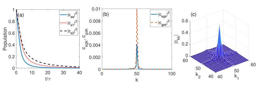
Figure 2: The evolution of two atoms coupled with a waveguide.

For typical chiral interactions between the atoms and the waveguide, by Theorem 1 asymptotically there are two photons in the waveguide and the atoms are in their ground states. However, under certain extreme conditions, it may happen that there is only one photon in the waveguide and one atom is in the excited state persistently.

Theorem 2.

When $\gamma_{1R}=\gamma_{1L}$, $z_{1}=\frac{n\pi}{\omega_{a}}\ll c$ for some positive integer $n$, $z_{2}\ll c$, $\gamma_{2R}>\gamma_{2L}=0$ or $\gamma_{2L}>\gamma_{2R}=0$, the first atom holds a significant amount of excitation and the second atom decays to the ground state.

Proof.

We look at the case $\gamma_{2L}>\gamma_{2R}=0$. The other case $\gamma_{2L}>\gamma_{2R}=0$ can be proved similarly. Under the assumptions in Theorem 2, Eqs. (8,9,10) become

$$\left\{\begin{aligned} &\dot{c}_{ee}(t)=-\frac{\gamma_{2L}^{2}+\gamma_{1R}^{2}+\gamma_{1L}^{2}}{2}c_{ee}(t)+\gamma_{1L}\gamma_{1R}c_{ee}(t-\frac{2z_{1}}{c})e^{i\omega_{a}\frac{2z_{1}}{c}},\\ &\dot{c}_{gek}(t,k)=-ic_{ee}(t)g_{k1t}(k,t,z_{1})-\frac{\gamma_{2L}^{2}}{2}c_{gek}(t,k),\\ &\dot{c}_{egk}(t,k)=-ic_{ee}(t)g_{k2t}(k,t,z_{2})-\frac{\gamma_{1R}^{2}+\gamma_{1L}^{2}}{2}c_{egk}(t,k)+\gamma_{1L}\gamma_{1R}c_{egk}(t-\frac{2z_{1}}{c},k)e^{i\omega_{a}\frac{2z_{1}}{c}}\\ &~{}~{}~{}~{}~{}~{}~{}~{}~{}~{}~{}~{}~{}~{}~{}+\gamma_{1R}\gamma_{2L}c_{gek}(t-\frac{z_{1}+z_{2}}{c},k)e^{i\omega_{a}\frac{z_{1}+z_{2}}{c}}-\gamma_{1L}\gamma_{2L}c_{gek}(t-\frac{z_{2}-z_{1}}{c},k)e^{i\omega_{a}\frac{z_{2}-z_{1}}{c}}.\\ \end{aligned}\right.$$ (16)

Applying the Laplace transform to the first two equations of (16) yields

$$~{}~{}~{}~{}C_{ee}(s)=\frac{1}{s+\frac{\gamma_{2L}^{2}+\gamma_{1R}^{2}+\gamma_{1L}^{2}}{2}-\gamma_{1L}\gamma_{1R}e^{i\omega_{a}\frac{2z_{1}}{c}}e^{-\frac{2z_{1}}{c}s}}.$$ (17)

By the final-value theorem,

$$~{}~{}~{}~{}\lim_{t\rightarrow\infty}c_{ee}(t)=\lim_{s\rightarrow 0}sC_{ee}(s)=\lim_{s\rightarrow 0}\frac{s}{s+\frac{\gamma_{2L}^{2}+\gamma_{1R}^{2}+\gamma_{1L}^{2}}{2}-\gamma_{1L}\gamma_{1R}e^{i\omega_{a}\frac{2z_{1}}{c}}e^{-\frac{2z_{1}}{c}s}}=0.$$ (18)

As a result, in the long-time limit, $\dot{c}_{gek}(t,k)\approx-\frac{\gamma_{2L}^{2}}{2}c_{gek}(t,k)$, and hence $\lim_{t\rightarrow\infty}c_{gek}(t,k)=0$. When $z_{1}=\frac{n\pi}{\omega_{a}}$, the third equation of Eq. (16) can be simplified when $t>t_{1}$ as

$$\dot{c}_{egk}(t,k)\approx-\frac{\gamma_{1R}^{2}+\gamma_{1L}^{2}}{2}c_{egk}(t,k)+\gamma_{1L}\gamma_{1R}c_{egk}(t-\frac{2z_{1}}{c},k)e^{i\omega_{a}\frac{2z_{1}}{c}},$$ (19)

because $c_{ee}(t)\approx 0$ and $c_{gek}(t,k)\approx 0$. For the evolution of $c_{egk}(t,k)$ when $t>t_{1}$ for some $t_{1}$ large enough, the Laplace transformation of Eq. (19) reads

$$sC_{egk}(s,k)-c_{egk}(t_{1},k) =-\frac{\gamma_{1R}^{2}+\gamma_{1L}^{2}}{2}C_{egk}(s,k)+\gamma_{1L}\gamma_{1R}C_{egk}(s,k)e^{-\frac{2z_{1}s}{c}}e^{i\omega_{a}\frac{2z_{1}}{c}}$$ (20)

$$\approx-\frac{\gamma_{1R}^{2}+\gamma_{1L}^{2}}{2}C_{egk}(s,k)+\gamma_{1L}\gamma_{1R}C_{egk}(s,k)e^{i\omega_{a}\frac{2z_{1}}{c}}.$$

Then

$$C_{egk}(s,k)\approx\frac{c_{egk}(t_{1},k)}{s+\frac{\gamma_{1R}^{2}+\gamma_{1L}^{2}}{2}-\gamma_{1L}\gamma_{1R}e^{i\omega_{a}\frac{2z_{1}}{c}}}.$$ (21)

Thus when $\gamma_{1L}=\gamma_{1R}$ and $\omega_{a}\frac{2z_{1}}{c}=2n\pi$, then $c_{egk}(t,k)\approx c_{egk}(t_{1},k)$.

We use Fig. 3 to demonstrate Theorem 2, where $z_{1}=\frac{\pi}{\omega_{a}}$, $z_{2}=\frac{2\pi}{\omega_{a}}$, $\gamma_{1L}=\gamma_{1R}=0.25$, $\gamma_{2L}=0.5$, $\gamma_{2R}=0$, and $\omega_{a}=50$. As shown in Fig. 3(a), the population $|c_{ee}(t)|^{2}$ converges to zero, while the population $|c_{e1}(t)|^{2}$ that the first atom is excited remains around $0.86$. As can be seen in Fig. 3(b), the amplitude of the single photon state $c_{egk}$ approximates a bump function at $\omega=\omega_{a}$ and $t=40\tau$. Finally, as can be seen from Fig. 3(c) that there are not observable two-photon states in the waveguide for $t=40\tau$.

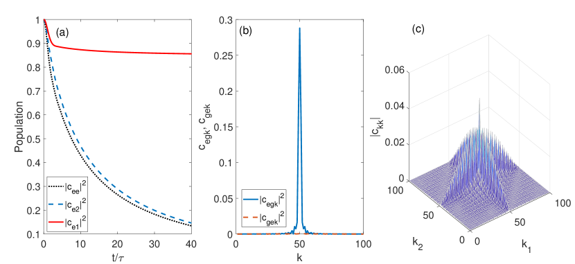
Figure 3: Control performance of the generation of the single photon state.

For the nonchiral case, we have the following result.

Theorem 3.

For the nonchiral waveguide, when $z_{j}=\frac{n\pi}{\omega_{a}}\ll c$, where $n=0,1,2,\cdots$, $j=1,2$, $c_{ee}(t)\approx 1$ .

Proof.

For the nonchiral waveguide, $\gamma_{jR}=\gamma_{jL}$. When $z_{j}=\frac{n\pi}{\omega_{a}}\ll c$ with $n=0,1,2,\cdots$ and $j=1,2$, then $-\gamma_{RL}+\gamma_{1L}\gamma_{1R}\cos(\omega_{a}\frac{2z_{1}}{c})+\gamma_{2L}\gamma_{2R}\cos(\omega_{a}\frac{2z_{2}}{c})\approx 0$ because $\sin(\omega_{a}\frac{2z_{j}}{c})=0$ and $\cos(\omega_{a}\frac{2z_{j}}{c})=1$ in Eq. (12). As a result, $c_{ee}(t)\approx 1$.

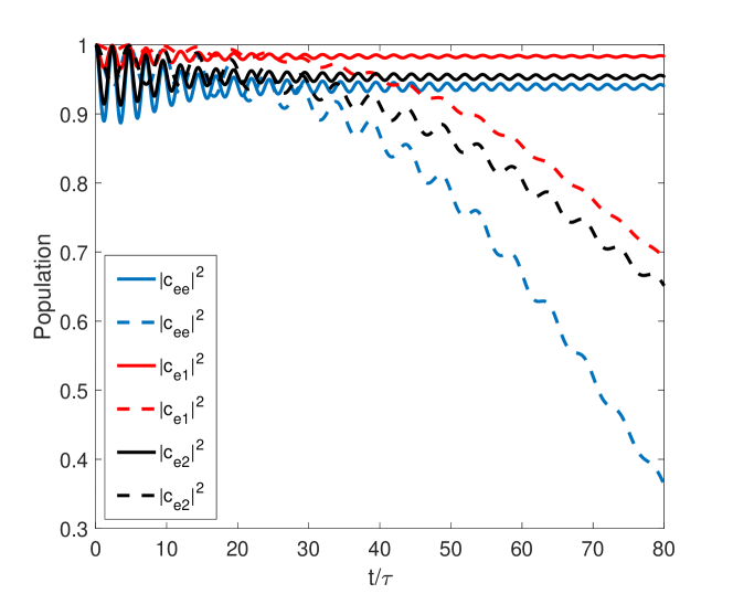
Figure 4: Comparison of the influence of atoms’ locations on the excited states.

As compared in Fig.4, the solid lines represent the simulations when $z_{1}=\frac{\pi}{\omega_{a}}$ and $z_{2}=\frac{2\pi}{\omega_{a}}$, and the dashed lines represent that $z_{1}=\frac{\pi}{2\omega_{a}}$ and $z_{2}=\frac{3\pi}{2\omega_{a}}$. In both of the above simulations, $\omega_{a}=50$, $\gamma_{jR}=\gamma_{jL}=0.5$. The comparisons agree with the conclusions in Theorem 3 that when the locations of the two charily coupled atoms are $z_{j}=\frac{n\pi}{\omega_{a}}$, $n=1,2,\cdots$, $j=1,2$, as the solid lines in Fig.4, the two atoms maintain their excited states due to the coherent feedback interactions.

Remark 1.

The conclusion of Theorem 2 and Theorem 3 reveals that the coherent feedback network can maintain the excited one or two atoms by tuning the location of atoms and the chiral coupling strengths between the atoms and waveguide. In Theorem 2, the atom is highly excited with photon packet in the waveguide is called the atom-photon bound state usually with population trappings, which has been introduced based on the coherent feedback network that one two-level atom is nonchirally coupled with a semi-infinite waveguide in Ref. [68]. In Theorem 3, both of the two atoms are excited with no photons in the waveguide, which constructs the dark state of the system and is a generalization of the one-atom circumstance in Ref. [71]. This is meaningful because it can enhance the lifetime of the qubits by elongating the duration of the excited states. This also provides a new method to generate the trapped excited quantum states through coherent feedback design.

Above all, based on the coherent feedback network that two atoms coupled with a semi-infinite waveguide, the number of photons in the waveguide can be controlled by tuning the chirally coupling strengths between the atom and waveguide as well as the locations of the atoms, which makes it possible to generate zero-photon, one-photon and two-photon states in the waveguide.

3 The feedback analysis in the spatial domain

The number of photons in the waveguide can be studied by means of the delay-dependent feedback equation (7). However, the spatial distribution of photons in the waveguide can only be studied by modeling in the spatial domain. The Hamiltonian of the waveguide in the frequency domain is given by the second term on the right-hand side of Eq. (5), whose spatial domain counterpart is [62, 59]

$$H_{w}=iv_{g}\int_{0}^{\infty}dzc_{L}^{{\dagger}}(z)\frac{\partial}{\partial z}c_{L}(z)-iv_{g}\int_{0}^{\infty}dzc_{R}^{{\dagger}}(z)\frac{\partial}{\partial z}c_{R}(z),$$ (22)

where $v_{g}$ is the group velocity of the photon wave packet in the waveguide, $c_{L}^{{\dagger}}(z)$ and $c_{L}(z)$ are the creation and annihilation operators for the left-propagating field at the position $z$, and $c_{R}^{{\dagger}}(z)$ and $c_{R}(z)$ are those for the right-propagating field. More details on Eq. (22) are given in Appendix B.

In subsection 3.1, we analyze the chiral feedback dynamics when there is a single atom coupled with a semi-infinite waveguide. Then we generalize to the two-atom case in subsection 3.2.

3.1 One atom coupled with the waveguide

When there is only the first atom at $z=z_{1}$ in Fig. 1 coupled with the waveguide, namely $\gamma_{2L}=\gamma_{2R}=0$, the quantum state for this one-exciton case is of the format

$$|\Psi(t)\rangle=\int_{0}^{\infty}dz\;\Phi_{R}(z,t)e^{-i\omega_{1}t}|1_{z}^{r},g\rangle+\int_{0}^{\infty}dz\;\Phi_{L}(z,t)e^{-i\omega_{1}t}|1_{z}^{l},g\rangle+c_{e}(t)e^{-i\omega_{2}t}|0,e\rangle,$$ (23)

where $|1_{z}^{r,l},g\rangle$ means that the first atom is at the ground state and the right or left-propagating photon can be detected at the position $z$, $|0,e\rangle$ means that the first atom is excited and the waveguide is empty, $\Phi_{R}(z,t)$ denotes the amplitude of the right-propagating photon wavepacket at the position $z$, $\Phi_{L}(z,t)$ is the amplitude of a left-propagating photon wavepacket, $c_{e}(t)$ is the amplitude that the first atom is excited, and $\tilde{\omega}_{1}$ and $\tilde{\omega}_{2}$ are the eigenfrequencies of the ground and excited state respectively with $\omega_{a}=\tilde{\omega}_{2}-\tilde{\omega}_{1}$.

The Hamiltonian of the whole quantum system reads

$$H=\tilde{\omega}_{1}|g\rangle\langle g|+\tilde{\omega}_{2}|e\rangle\langle e|+H_{w}+H_{m}+H_{I},$$ (24)

where the waveguide Hamiltonian $H_{w}$ is given in Eq. (22), the mirror Hamiltonian $H_{m}$ and the interaction Hamiltonian $H_{I}$ are given in Eqs. (56) and (53) in Appendix B, respectively.

Solving the Schrödinger equation $\frac{\partial}{\partial t}|\Psi(t)\rangle=-iH|\Psi(t)\rangle$ with $H$ in Eq. (24) and the ansatz $|\Psi(t)\rangle$ in Eq. (23), we get a system of partial differential equations (PDEs) of the form

$$\dot{c}_{e}(t)=-\left[\gamma_{1R}\Phi_{R}(z_{1},t)+\gamma_{1L}\Phi_{L}(z_{1},t)\right]e^{i\omega_{a}t},$$ (25a)

$$\frac{\partial\Phi_{R}(z,t)}{\partial t}=-v_{g}\frac{\partial\Phi_{R}(z,t)}{\partial z}+2v_{g}\delta(z)\Phi_{L}(z,t)e^{i2kz}+\gamma_{1R}\delta(z-z_{1})c_{e}(t)e^{-i\omega_{a}t},$$ (25b)

$$\frac{\partial\Phi_{L}(z,t)}{\partial t}=v_{g}\frac{\partial\Phi_{L}(z,t)}{\partial z}-2v_{g}\delta(z)\Phi_{R}(z,t)e^{-2ikz}+\gamma_{1L}\delta(z-z_{1})c_{e}(t)e^{-i\omega_{a}t},$$ (25c)

where Eq. (25a) means that the excited atom can emit a single photon into the waveguide along the right or left direction, and the probability is determined by the chiral coupling strengths between the atom and the waveguide; Eq. (25b) shows that the right-propagating mode is determined by the reflection of the mirror from the left-propagating mode at $z=0$, the position of the atom, and the coupling strength between the atom and the waveguide along the right direction; Eq. (25c) further shows that the left-propagating mode can be influenced by the coupling strength between the atom and the waveguide along the left direction.

Remark 2.

One of the advantages of representing the evolution of the quantum system as formula (25) in the spatial domain is that the differential of the excited atomic state is directly represented with the spatial distribution of the photon states rather than their integrations as in Eq. (7).

The quantum state with one right- or left propagating photon in the waveguide $\Phi_{R}(z,t)$ and $\Phi_{L}(z,t)$ in Eq. (23) can be represented according to the position as

$$\Phi_{R}(z,t)=[\Theta(z)-\Theta(z-z_{1})]f_{r}(t-z/c)+\Theta(z-z_{1})g_{r}(t-z/c),$$ (26a)

$$\Phi_{L}(z,t)=[\Theta(z)-\Theta(z-z_{1})]f_{l}(t+z/c),$$ (26b)

respectively, where $\Theta$ represents the Heaviside step function, $f_{r}(t-z/c)$ represents the right-propagating photonic mode in the area $0<z<z_{1}$, $g_{r}(t-z/c)$ is that in the area $z>z_{1}$, and $f_{l}(t+z/c)$ represents the left-propagating photonic mode in the area $0<z<z_{1}$ [59].

According to the calculations in Appendix C, Eq. (25a) can be written in the delay-dependent form as

$$\dot{c}_{e}(t)=-\frac{\gamma_{1R}^{2}+\gamma_{1L}^{2}}{2v_{g}}c_{e}(t)+\frac{\gamma_{1L}\gamma_{1R}}{v_{g}}c_{e}(t-2z_{1}/c)e^{i2\omega_{a}z_{1}/c}.$$ (27)

Let the atom be initialized in the excited state, i.e., $c_{e}(0)=1$, and take $v_{g}=c=1$. Laplace transforming Eq. (27) yields

$$sC_{e}(s)-1=-\frac{\gamma_{1R}^{2}+\gamma_{1L}^{2}}{2}C_{e}(s)+\gamma_{1L}\gamma_{1R}C_{e}(s)e^{-2\frac{z_{1}}{c}s}e^{i2\omega_{a}z_{1}/c}.$$ (28)

We have

$$C_{e}(s) =\frac{1}{s-\gamma_{1L}\gamma_{1R}e^{-2\frac{z_{1}}{c}s}e^{i2\omega_{a}z_{1}/c}+\frac{\gamma_{1R}^{2}+\gamma_{1L}^{2}}{2}},$$ (29)

which agrees with the form of Eq. (8) with $\gamma_{2R}=\gamma_{2L}=0$.

Theorem 4.

When $\gamma_{1R}=\gamma_{1L}$, and $z_{1}=\frac{n}{\omega_{a}}\pi\ll c$, where $n$ is an integer satisfying that $\frac{n}{\omega_{a}}\ll c$, the atom at $z_{1}$ can be always excited.

Proof.

When $\gamma_{1R}=\gamma_{1L}$, and $z_{1}=\frac{n}{\omega_{a}}\pi\ll c$, $-\gamma_{1L}\gamma_{1R}e^{-2\frac{z_{1}}{c}s}e^{i\omega_{a}\tau_{1}}+\frac{\gamma_{1R}^{2}+\gamma_{1L}^{2}}{2}\approx\frac{\gamma_{1R}^{2}+\gamma_{1L}^{2}}{2}-\gamma_{1L}\gamma_{1R}=0$. Then

$$C_{e}(s)=\frac{1}{s-\gamma_{1L}\gamma_{1R}e^{-2\frac{z_{1}}{c}s}+\frac{\gamma_{1R}^{2}+\gamma_{1L}^{2}}{2}}\approx\frac{1}{s-\gamma_{1L}\gamma_{1R}+\frac{\gamma_{1R}^{2}+\gamma_{1L}^{2}}{2}}=\frac{1}{s},$$ (30)

and $\lim_{t\rightarrow\infty}c_{e}(t)=\lim_{s\rightarrow 0}sC_{e}(s)=1$.

In the above, we generalized the control performance that the atom is nonchirally coupled with the waveguide in Ref. [59] to that the atom is chirally coupled with the waveguide. To compare with the result in Ref. [59], where the mirror is at the right terminal of the waveguide, we first derive its counterpart when the mirror is at the left terminal of the waveguide. After that we compare the populations of the excited atomic state and the right propagating single-photon wave packet. The performances with $z_{1}=\frac{2.25\pi}{\omega_{a}}$ and $\omega_{a}=50$ are given in Fig. 5, where (a) is for the population $|c_{e}(t)|^{2}$ and (b) is for the right-propagating photon wave packet solved in Appendix C.For the nonchiral coupling as in Ref. [59], we take $\gamma_{1R}=\gamma_{1L}=0.2$, while we let $\gamma_{1R}=3\gamma_{1L}=0.3$ and $\gamma_{1R}=7\gamma_{1L}=0.35$ for the chiral couplings respectively. Here for the simulations of the right-propagating photon wave packet, $g_{r}(t-z/c)$ is given by replacing $t$ in the right hand side of Eq. (69) with $t-z/c$. The simulations that $\gamma_{1R}<\gamma_{1L}$ are similar with the circumstance that $\gamma_{1R}>\gamma_{1L}$.

Remark 3.

In the parameters settings in Fig. 5, $e^{i2\omega_{a}z_{1}/c}=i$ and $\gamma_{1L}+\gamma_{1R}=0.4$, $|c_{e}(t)|^{2}=e^{-(\gamma_{1L}^{2}+\gamma_{1R}^{2})t}\leq e^{-\frac{(\gamma_{1L}+\gamma_{1R})^{2}}{2}t}$ with the equality established only when $\gamma_{1L}=\gamma_{1R}$. Thus the chiral coupling can induce faster decaying of the excited atomic state.

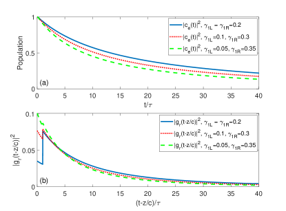
Figure 5: Comparison of the feedback control with chiral coupling and nonchiral coupling (in Ref. [59]) between one atom and the semi-infinite waveguide.

The conclusion in Theorem 4 agrees with the analysis in the frequency domain in Ref. [68], which clarifies that at the exact parameter setting of the location of the first atom, there will not be any photons emitted into the waveguide and the atom functions as an atomic mirror. Considering that Theorem 4 holds only when the interaction between the atom and the waveguide is nonchiral, this can also be derived from the nonchiral model in Ref. [59].

3.2 Two atoms coupled with the waveguide

When there are two atoms coupled with the semi-infinite waveguide, the Hamiltonian for the two-atom case, as the counterpart of that in Eq.(24) for the single-atom case, reads

$$H=\sum_{j=1,2}(\hbar\tilde{\omega}_{1}|g_{j}\rangle\langle g_{j}|+\hbar\tilde{\omega}_{2}|e_{j}\rangle\langle e_{j}|)+H_{w}+H_{m}+\sum_{j=1,2}H_{I}^{j},$$ (31)

where $H_{w}$ and $H_{m}$ are given in Eq. (24), and $H_{I}^{j}$ is generalized from Eq. (53) as

$$H_{I}^{j}=-i\int_{-\infty}^{\infty}\mathrm{d}z[\gamma_{jR}c_{R}(z)\delta(z-z_{j})+\gamma_{jL}c_{L}(z)\delta(z-z_{j})]\sigma_{j}^{+}+\mathrm{H.c.},\ \ j=1,2.$$ (32)

We assume initially only the first atom is excited, and there can be at most one photon in the waveguide. Then the quantum state can be represented as

$$|\Psi(t)\rangle=\sum_{j=1,2}c_{j}(t)e^{-i\left(\tilde{\omega}_{1}+\tilde{\omega}_{2}\right)t}\sigma_{j}^{+}|g_{1},g_{2},\{0\}\rangle+\int_{0}^{\infty}\Phi_{g}^{l}(t,z)e^{-i2\tilde{\omega}_{1}t}|g_{1},g_{2},1_{z}^{r}\rangle\mathrm{d}z+\int_{0}^{\infty}\Phi_{g}^{l}(t,z)e^{-i2\tilde{\omega}_{1}t}|g_{1},g_{2},1_{z}^{l}\rangle\mathrm{d}z,$$ (33)

where $c_{j}(t)$ represents the amplitude that the $j$th atom is excited and there is not any photons in the waveguide, $\Phi_{g}^{r}(t,z)$ and $\Phi_{g}^{l}(t,z)$ represent the amplitudes of the states that both of the two atoms are in the ground state and there is one right or left-propagating photon in the waveguide respectively. Take the state representation into the Schrödinger equation and we have

$$\dot{c}_{j}(t)=-\gamma_{jR}\Phi_{g}^{r}(t,z_{j})e^{i\omega_{a}t}-\gamma_{jL}\Phi_{g}^{l}(t,z_{j})e^{i\omega_{a}t},$$ (34a)

$$\frac{\partial\Phi_{g}^{r}(t,z)}{\partial t}=-v_{g}\frac{\partial\Phi_{g}^{r}(t,z)}{\partial z}+2v_{g}\Phi_{g}^{l}(t,z)e^{2ikz}\delta(z)+\sum_{j=1,2}\gamma_{jR}c_{j}(t)\delta(z-z_{j})e^{-i\omega_{a}t},$$ (34b)

$$\frac{\partial\Phi_{g}^{l}(t,z)}{\partial t}=v_{g}\frac{\partial\Phi_{g}^{l}(t,z)}{\partial z}-2v_{g}\Phi_{g}^{r}(t,z)e^{-2ikz}\delta(z)+\sum_{j=1,2}\gamma_{jL}c_{j}(t)\delta(z-z_{j})e^{-i\omega_{a}t}.$$ (34c)

$\Phi_{g}^{R}(t,z)$ and $\Phi_{g}^{l}(t,z)$ can be further represented as

$$\Phi_{g}^{r}(z,t)=\left[\Theta(z)-\Theta(z-z_{1})\right]f_{r}(t-z/c)+\left[\Theta(z-z_{1})-\Theta(z-z_{2})\right]g_{r}(t-z/c)+\Theta(z-z_{2})h_{r}(t-z/c),$$ (35a)

$$\Phi_{g}^{l}(z,t)=\left[\Theta(z)-\Theta(z-z_{1})\right]f_{l}(t+z/c)+\left[\Theta(z-z_{1})-\Theta(z-z_{2})\right]g_{l}(t+z/c),$$ (35b)

where $f_{r}(t-z/c)$, $g_{r}(t-z/c)$ and $h_{r}(t-z/c)$ represent the right-propagating photon wave packets at $[0,z_{1}]$, $[z_{1},z_{2}]$ and $[z_{2},+\infty]$, $f_{l}(t+z/c)$ and $g_{l}(t+z/c)$ are for the left-propagating photon wave packets at $[0,z_{1}]$ and $[z_{1},z_{2}]$, respectively.

The $c_{j}(t)$ with $j=1,2$ can be solved in the spatial domain as illustrated in Appendix  D, which agrees with the analysis in the frequency domain in Ref. [49]. While the spatial distribution of the photon wave packet can be clarified based on Eq. (34) and solved as Eq. (78), which cannot be covered in the frequency domain analysis. As compared in Fig. 6 (a) with $z_{2}=10z_{1}=10$ and $\omega_{a}=50$, the first atom decays via the spontaneous emission, and the emitted photon can further excite the second atom after the direct transmission or the reflection by the mirror. As a result, the second atom can be transiently more exited by the right-propagating photon wave packet emitted by the first atom, especially when $\gamma_{2R}$ is much larger than $\gamma_{2L}$. The right propagating photon wave packets at $z>z_{2}$ are compared in Fig. 6 (b) by combining Eqs. (78c,78d,78e), which is influenced by the locations of the atoms and the reflection of the mirror.

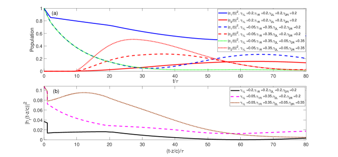
Figure 6: Comparison of the feedback control of two atoms with one excitation.

4 Conclusion

In this paper, we have analyzed the coherent feedback control with photons upon the architecture that two atoms are chirally coupled with the semi-infinite waveguide. When the atoms are initially excited, the number of generated photons in the waveguide is influenced by the locations of the atoms and there chiral coupling strengths with different directional propagating modes in the waveguide. Once the locations of the atoms and their chiral coupling strengths with the waveguide are well designed, two-photon, one-photon and zero-photon states can be generated in the waveguide. Additionally, the spatial modeling of the quantum system provides another approach to clarify dynamics of the two atoms coupled with the waveguide, and the example of the one-atom and two-atom cases can provide the comprehensive analysis when combined with the frequency domain modeling.

Appendix

Appendix A Derivations of Eqs. (8,9,10)

In this appendix, we derive Eqs. (8,9,10), which demonstrate clearly the influence of the round-trip delays in the coherent feedback network in Fig. 1 on its dynamics.

(1) Derivation of Eq. (9).

For the second component on the right hand side of Eq. (7b), $c_{kk}(k,k_{1},t)$ can be replaced with the integration of Eq. (7d); specifically,

$$~{}~{}~{}~{}-i\int c_{kk}(k,k_{1},t)g_{k1t}^{*}(k_{1},t,z_{1})\mathrm{d}k_{1}$$ (36)

$$=-\int_{0}^{t}du\int[c_{egk}(u,k)g_{k1t}(k_{1},u,z_{1})+c_{egk}(u,k_{1})g_{k1t}(k,u,z_{1})$$

$$~{}~{}~{}~{}+c_{gek}(u,k)g_{k2t}(k_{1},u,z_{2})+c_{gek}(u,k_{1})g_{k2t}(k,u,z_{2})]g_{k1t}^{*}(k_{1},t,z_{1})\mathrm{d}k_{1}.$$

Noticing that

$$~{}~{}~{}~{}\int c_{egk}(u,k)g_{k1t}(k_{1},u,z_{1})g_{k1t}^{*}(k_{1},t,z_{1})\mathrm{d}k_{1}$$ (37)

$$=\int c_{egk}(u,k)\left[\gamma_{1R}^{2}e^{i(\omega_{1}-\omega_{a})(u-t)}-\gamma_{1L}\gamma_{1R}e^{i[(\omega_{1}-\omega_{a})(u-t)+2\omega_{1}z_{1}/c]}-\gamma_{1R}\gamma_{1L}e^{i[(\omega_{1}-\omega_{a})(u-t)-2\omega_{1}z_{1}/c]}+\gamma_{1L}^{2}e^{i(\omega_{1}-\omega_{a})(u-t)}\right]\mathrm{d}k_{1}$$

$$=\int c_{egk}(u,k)e^{-i\omega_{a}(u-t)}\left[\gamma_{1R}^{2}e^{i\omega_{1}(u-t)}-\gamma_{1L}\gamma_{1R}e^{i\omega_{1}(u-t+2z_{1}/c)}-\gamma_{1R}\gamma_{1L}e^{i\omega_{1}(u-t-2z_{1}/c)}+\gamma_{1L}^{2}e^{i\omega_{1}(u-t)}\right]\mathrm{d}k_{1}$$

$$=c_{egk}(u,k)e^{-i\omega_{a}(u-t)}\left[\gamma_{1R}^{2}\delta(u-t)-\gamma_{1L}\gamma_{1R}\delta(u-t+2z_{1}/c)-\gamma_{1R}\gamma_{1L}\delta(u-t-2z_{1}/c)+\gamma_{1L}^{2}\delta(u-t)\right].$$

Thus the first component in Eq. (36) becomes

$$~{}~{}~{}~{}\int_{0}^{t}du\int c_{egk}(u,k)g_{k1t}(k_{1},u,z_{1})g_{k1t}^{*}(k_{1},t,z_{1})\mathrm{d}k_{1}$$ (38)

$$=\int_{0}^{t}du\;c_{egk}(u,k)e^{-i\omega_{a}(u-t)}\left[\gamma_{1R}^{2}\delta(u-t)-\gamma_{1L}\gamma_{1R}\delta(u-t+2z_{1}/c)-\gamma_{1R}\gamma_{1L}\delta(u-t-2z_{1}/c)+\gamma_{1L}^{2}\delta(u-t)\right]$$

$$=\frac{\gamma_{1R}^{2}+\gamma_{1L}^{2}}{2}c_{egk}(t,k)-\gamma_{1L}\gamma_{1R}c_{egk}(t-2z_{1}/c,k)e^{i\omega_{a}\frac{2z_{1}}{c}},$$

which means that the temporal evolution of $c_{egk}(t,k)$ is influenced not only by the chiral coupling strengths, but also by the round-trip delay between the first atom and the mirror.

For the second component in Eq. (36), we have

$$~{}~{}~{}~{}\int c_{egk}(u,k_{1})g_{k1t}(k,u,z_{1})g_{k1t}^{*}(k_{1},t,z_{1})\mathrm{d}k_{1}$$ (39)

$$=\int c_{egk}(u,k_{1})\left[i\gamma_{1R}e^{i[(\omega-\omega_{a})u-\omega z_{1}/c]}-i\gamma_{1L}e^{i[(\omega-\omega_{a})u+\omega z_{1}/c]}\right]\left[-i\gamma_{1R}e^{-i[(\omega_{1}-\omega_{a})t-\omega_{1}z_{1}/c]}+i\gamma_{1L}e^{-i[(\omega_{1}-\omega_{a})t+\omega_{1}z_{1}/c]}\right]\mathrm{d}k_{1},$$

which equals zero according to the following lemma.

Lemma 1.

For the finite amplitude $c_{egk}(u,k_{1})$ which is a continuous function of the time variable $u$, we have

$$\int c_{egk}(u,k_{1})e^{-i[(\omega_{1}-\omega_{a})t-\omega_{1}z_{1}/c]}\mathrm{d}k_{1}=0.$$

Proof.

Notice that

$$~{}~{}~{}~{}\int c_{egk}(u,k_{1})e^{-i[(\omega_{1}-\omega_{a})t-\omega_{1}z_{1}/c]}\mathrm{d}k_{1}$$ (40)

$$=e^{i\omega_{a}t}\int c_{egk}(u,k_{1})e^{-i\omega_{1}(t-z_{1}/c)}\mathrm{d}k_{1}$$

$$=e^{i\omega_{a}t}\left[\int e^{-i\omega_{1}(t-z_{1}/c)}\mathrm{d}k_{1}c_{egk}(u,k_{1})-\int\int e^{-i\omega_{1}^{\prime}(t-z_{1}/c)}\mathrm{d}k_{1}^{\prime}\frac{dc_{egk}(u,k_{1})}{dk_{1}}\mathrm{d}k_{1}\right]$$

$$=e^{i\omega_{a}t}\left[\delta(t-z_{1}/c)c_{egk}(u,k_{1})-\int\delta(t-z_{1}/c)\frac{dc_{egk}(u,k_{1})}{dk_{1}}\mathrm{d}k_{1}\right].$$

When $t\neq z_{1}/c$, $\delta(t-z_{1}/c)=0$, consequently $\int c_{egk}(u,k_{1})e^{-i[(\omega_{1}-\omega_{a})t-\omega_{1}z_{1}/c]}\mathrm{d}k_{1}=0$. Because $c_{egk}$ is continuous, $\int c_{egk}(u,k_{1})e^{-i[(\omega_{1}-\omega_{a})t-\omega_{1}z_{1}/c]}\mathrm{d}k_{1}=0$ for arbitrary $u$.

For the third component of Eq. (36), the integration with respect to $k_{1}$ is

$$~{}~{}~{}~{}\int c_{gek}(u,k)g_{k2t}(k_{1},u,z_{2})g_{k1t}^{*}(k_{1},t,z_{1})\mathrm{d}k_{1}$$ (41)

$$=c_{gek}(u,k)\int\Big{[}\gamma_{1R}\gamma_{2R}e^{i[(\omega_{1}-\omega_{a})(u-t)-\omega_{1}(z_{2}-z_{1})/c]}-\gamma_{1R}\gamma_{2L}e^{i[(\omega_{1}-\omega_{a})(u-t)+\omega_{1}(z_{1}+z_{2})/c]}$$

$$~{}~{}~{}~{}-\gamma_{2R}\gamma_{1L}e^{i[(\omega_{1}-\omega_{a})(u-t)-\omega_{1}(z_{2}+z_{1})/c]}+\gamma_{1L}\gamma_{2L}e^{i[(\omega_{1}-\omega_{a})(u-t)+\omega_{1}(z_{2}-z_{1})/c]}\Big{]}\mathrm{d}k_{1}$$

$$=c_{gek}(u,k)e^{-i\omega_{a}(u-t)}\int\Big{[}\gamma_{1R}\gamma_{2R}e^{i\omega_{1}[u-t-(z_{2}-z_{1})/c]}-\gamma_{1R}\gamma_{2L}e^{i\omega_{1}[u-t+(z_{1}+z_{2})/c]}$$

$$~{}~{}~{}~{}-\gamma_{2R}\gamma_{1L}e^{i\omega_{1}[u-t-(z_{2}+z_{1})/c]}+\gamma_{1L}\gamma_{2L}e^{i\omega_{1}[u-t+(z_{2}-z_{1})/c]}\Big{]}\mathrm{d}k_{1}$$

$$=c_{gek}(u,k)e^{-i\omega_{a}(u-t)}\Big{[}\gamma_{1R}\gamma_{2R}\delta(u-t-\frac{z_{2}-z_{1}}{c})-\gamma_{1R}\gamma_{2L}\delta(u-t+\frac{z_{1}+z_{2}}{c})$$

$$~{}~{}~{}~{}-\gamma_{2R}\gamma_{1L}\delta(u-t-\frac{z_{2}+z_{1}}{c})+\gamma_{1L}\gamma_{2L}\delta(u-t+\frac{z_{2}-z_{1}}{c})\Big{]}.$$

Then the third component of Eq. (36) reads

$$~{}~{}~{}~{}\int_{0}^{t}du\int c_{gek}(u,k)g_{k2t}(k_{1},u,z_{2})g_{k1t}^{*}(k_{1},t,z_{1})\mathrm{d}k_{1}$$ (42)

$$=\int_{0}^{t}duc_{gek}(u,k)e^{-i\omega_{a}(u-t)}\left[-\gamma_{1R}\gamma_{2L}\delta(u-t+\frac{z_{1}+z_{2}}{c})+\gamma_{1L}\gamma_{2L}\delta(u-t+\frac{z_{2}-z_{1}}{c})\right]$$

$$=-\gamma_{1R}\gamma_{2L}c_{gek}(t-\frac{z_{1}+z_{2}}{c},k)e^{i\omega_{a}\frac{z_{1}+z_{2}}{c}}+\gamma_{1L}\gamma_{2L}c_{gek}(t-\frac{z_{2}-z_{1}}{c},k)e^{i\omega_{a}\frac{z_{2}-z_{1}}{c}}$$

Clearly, the first term is related to the delay (a left-propagating field is emitted by the second atom, and then is reflected by the mirror and interacts with the first atom), while the second term is related with the transmission delay from the second atom to the first atom.

Similar to the proof for Lemma 1, it can be shown that

$$\int c_{gek}(u,k_{1})g_{k2t}(k,u,z_{2})g_{k1t}^{*}(k_{1},t,z_{1})\mathrm{d}k_{1}=0.$$

Thus, the forth component of Eq. (36) equals zero.

In summary, the evolution of $c_{egk}(t,k)$ can be rewritten as:

$$\dot{c}_{egk}(t,k)=-ic_{ee}(t)g_{k2t}(k,t,z_{2})-\frac{\gamma_{1R}^{2}+\gamma_{1L}^{2}}{2}c_{egk}(t,k)+\gamma_{1L}\gamma_{1R}c_{egk}(t-2z_{1}/c,k)e^{i\omega_{a}\frac{2z_{1}}{c}}$$ (43)

$$+\gamma_{1R}\gamma_{2L}c_{gek}(t-\frac{z_{1}+z_{2}}{c},k)e^{i\omega_{a}\frac{z_{1}+z_{2}}{c}}-\gamma_{1L}\gamma_{2L}c_{gek}(t-\frac{z_{2}-z_{1}}{c},k)e^{i\omega_{a}\frac{z_{2}-z_{1}}{c}},$$

which is Eq. (9) in the main text.

(2) Derivation of Eq. (10).

The derivation of Eq. (10) is similar with that of Eq. (9), thus is omitted.

(3) Derivation of Eq. (8).

Take the integration of Eq. (43) into the former part of Eq. (7a),

$$~{}~{}~{}~{}\int c_{egk}(t,k)g_{k2t}^{*}(k,t,z_{2})\mathrm{d}k$$ (44)

$$=\int\int_{0}^{t}du\Big{\{}-ic_{ee}(u)g_{k2t}(k,u,z_{2})-\frac{\gamma_{1R}^{2}+\gamma_{1L}^{2}}{2}c_{egk}(u,k)+\gamma_{1L}\gamma_{1R}c_{egk}(u-2z_{1}/c,k)e^{i\omega_{a}\frac{2z_{1}}{c}}$$

$$+\gamma_{1R}\gamma_{2L}c_{gek}(u-\frac{z_{1}+z_{2}}{c},k)e^{i\omega_{a}\frac{z_{1}+z_{2}}{c}}-\gamma_{1L}\gamma_{2L}c_{gek}(u-\frac{z_{2}-z_{1}}{c},k)e^{i\omega_{a}\frac{z_{2}-z_{1}}{c}}\Big{\}}g_{k2t}^{*}(k,t,z_{2})\mathrm{d}k,$$

where the first inner integration reads

$$~{}~{}~{}~{}\int\int_{0}^{t}du\{-ic_{ee}(u)g_{k2t}(k,u,z_{2})g_{k2t}^{*}(k,t,z_{2})\mathrm{d}k$$ (45)

$$=-i\int_{0}^{t}c_{ee}(u)e^{-i\omega_{a}(u-t)}du\int\left[\gamma_{2R}^{2}e^{i\omega(u-t)}-\gamma_{2L}\gamma_{2R}e^{i\omega(u-t+\frac{2z_{2}}{c})}-\gamma_{2L}\gamma_{2R}e^{i\omega(u-t-\frac{2z_{2}}{c})}+\gamma_{2L}^{2}e^{i\omega(u-t)}\right]\mathrm{d}k$$

$$=-i\int_{0}^{t}c_{ee}(u)e^{-i\omega_{a}(u-t)}du\left[(\gamma_{2R}^{2}+\gamma_{2L}^{2})\delta(u-t)-\gamma_{2L}\gamma_{2R}\delta(u-t+\frac{2z_{2}}{c})-\gamma_{2L}\gamma_{2R}\delta(u-t-\frac{2z_{2}}{c})\right],$$

and the following integrations in Eq. (44) equal zero according to Lemma 1. Thus

$$~{}~{}~{}~{}\int c_{egk}(t,k)g_{k2t}^{*}(k,t,z_{2})\mathrm{d}k=-i\frac{\gamma_{2R}^{2}+\gamma_{2L}^{2}}{2}c_{ee}(t)+i\gamma_{2L}\gamma_{2R}c_{ee}(t-\frac{2z_{2}}{c})e^{i\omega_{a}\frac{2z_{2}}{c}}.$$ (46)

Similar for the latter part of Eq. (7a),

$$~{}~{}~{}~{}\int c_{gek}(t,k)g_{k1t}^{*}(k,t,z_{1})\mathrm{d}k=-i\left[\frac{\gamma_{1R}^{2}+\gamma_{1L}^{2}}{2}c_{ee}(t)-\gamma_{1L}\gamma_{1R}c_{ee}(t-\frac{2z_{1}}{c})e^{i\omega_{a}\frac{2z_{1}}{c}}\right].$$ (47)

Then the evolution of $c_{ee}(t)$ can be written as:

$$~{}~{}~{}~{}\dot{c}_{ee}(t)$$ (48)

$$=-i\left[-i\frac{\gamma_{2R}^{2}+\gamma_{2L}^{2}}{2}c_{ee}(t)+i\gamma_{2L}\gamma_{2R}c_{ee}(t-\frac{2z_{2}}{c})e^{i\omega_{a}\frac{2z_{2}}{c}}\right]-\left[\frac{\gamma_{1R}^{2}+\gamma_{1L}^{2}}{2}c_{ee}(t)-\gamma_{1L}\gamma_{1R}c_{ee}(t-\frac{2z_{1}}{c})e^{i\omega_{a}\frac{2z_{1}}{c}}\right]$$

$$=-\frac{\gamma_{1R}^{2}+\gamma_{1L}^{2}+\gamma_{2R}^{2}+\gamma_{2L}^{2}}{2}c_{ee}(t)+\gamma_{1L}\gamma_{1R}c_{ee}(t-\frac{2z_{1}}{c})e^{i\omega_{a}\frac{2z_{1}}{c}}+\gamma_{2L}\gamma_{2R}c_{ee}(t-\frac{2z_{2}}{c})e^{i\omega_{a}\frac{2z_{2}}{c}},$$

which is the format of Eq. (8) in the main text.

Appendix B Derivation of the interaction Hamiltonian in the spatial domain

When an atom is coupled with an infinite waveguide, the photon wave packet can be divided into the right-propagating and left-propagating components. Accordingly, the Hamiltonian of the waveguide mode, given by the second term on the right-hand side of Eq. (5) in the main text, can be divided into two counter-propagating parts as [59]:

$$\int_{0}^{\infty}\mathrm{d}k\;\omega_{k}d^{{\dagger}}_{k}d_{k}= \int_{0}^{\infty}\mathrm{d}k_{L}\;\omega_{k_{L}}d^{{\dagger}}_{k_{L}}d_{k_{L}}+\int_{0}^{\infty}\mathrm{d}k_{R}\;\omega_{k_{R}}d^{{\dagger}}_{k_{R}}d_{k_{R}},$$ (49)

where $d^{{\dagger}}_{k_{L}}(d_{k_{L}})$ represents the creation (annihilation) operator of the left-moving photonic wave packet, and $d^{{\dagger}}_{k_{R}}(d_{k_{R}})$ represents that of the right-moving photonic wave packet. Moreover, based on the linearization of the waveguide mode $\omega_{k}$ around $\omega_{0}$, the left- and right-propagating modes can be represented as [62, 72]:

$$\int_{0}^{\infty}\mathrm{d}k_{L}\;\omega_{k_{L}}d^{{\dagger}}_{k_{L}}d_{k_{L}}\simeq\int_{0}^{\infty}\mathrm{d}k_{L}\;[\omega_{0}-v_{g}(k_{L}-k_{0})]d^{{\dagger}}_{k_{L}}d_{k_{L}},$$ (50)

$$\int_{0}^{\infty}\mathrm{d}k_{R}\;\omega_{k_{R}}d^{{\dagger}}_{k_{R}}d_{k_{R}}\simeq\int_{0}^{\infty}\mathrm{d}k_{L}\;[\omega_{0}+v_{g}(k_{R}-k_{0})]d^{{\dagger}}_{k_{R}}d_{k_{R}},$$

where $v_{g}$ is the group velocity of the field, $\omega_{k_{L}}\simeq\omega_{0}-v_{g}(k_{L}-k_{0})$ and $\omega_{k_{R}}\simeq\omega_{0}+v_{g}(k_{R}-k_{0})$. The creation and annihilation operators $d_{k_{L}}^{{\dagger}}$ and $d_{k_{L}}$ for the left-propagating modes can be represented in terms of the spatial-domain operators:

$$\left\{\begin{aligned} &d_{k_{L}}^{{\dagger}}=\int_{-\infty}^{\infty}\mathrm{d}zc_{L}^{{\dagger}}(z)e^{ik_{L}z},\\ &d_{k_{L}}=\int_{-\infty}^{\infty}\mathrm{d}zc_{L}(z)e^{-ik_{L}z},\end{aligned}\right.$$ (51)

where $c_{L}^{{\dagger}}(z)$ and $c_{L}(z)$ are the creation and annihilation operators for the left-propagating field in the waveguide at position $z$, respectively. Similarly, for the right-propagating fields,

$$\left\{\begin{aligned} &d_{k_{R}}^{{\dagger}}=\int_{-\infty}^{\infty}\mathrm{d}zc_{R}^{{\dagger}}(z)e^{ik_{R}z},\\ &d_{k_{R}}=\int_{-\infty}^{\infty}\mathrm{d}zc_{R}(z)e^{-ik_{R}z},\end{aligned}\right.$$ (52)

with $c_{R}^{{\dagger}}(z)$ and $c_{R}(z)$ are the creation and annihilation operators for the right-propagating field in the waveguide at position $z$.

As for the chiral interaction part of the Hamiltonian, namely the last term on the right-hand side of Eq. (5) in the main text, the coupling is $g_{k1t}(k,t,z)$ given in Eq. (4). Based on the transformation between the frequency domain and the spatial domain in Eqs. (51,52), the interaction Hamiltonian in the spatial domain is  [62, 59]:

$$H_{I}=-i\int_{-\infty}^{\infty}\mathrm{d}z\left[\gamma_{1R}c_{R}(z)\delta(z-z_{1})+\gamma_{1L}c_{L}(z)\delta(z-z_{1})\right]\sigma_{1}^{+}+\mathrm{H.c.},$$ (53)

which gives the format of $H_{I}$ in Eq. (24) in the main text. See for more details please refer to Ref. [62].

B.1 The Hamiltonian of the mirror

The function of the mirror in Fig. 1 is to reflect a left-moving photon wavepacket to a right-moving wavepacket. Consider the circumstance that there are no atoms coupled with the waveguide. With the boundary of the mirror at $z=0$, the Hamiltonian of the system at the absence of the atoms is

$$H=H_{w}+H_{m},$$ (54)

where $H_{m}$ represents the Hamiltonian of the mirror and $H_{w}$ is the waveguide Hamiltonian given in Eq. (22). Let

$$|\Psi\rangle=\Theta(z)e^{ikz}c_{R}^{{\dagger}}(z)|0\rangle+\Theta(z)e^{-ikz}c_{L}^{{\dagger}}(z)|0\rangle,$$ (55)

where $\Theta$ represents the Heaviside step function.

Definition 1.

[59] The quantum state $|\Psi\rangle$ in Eq. (55) is called an eigenstate corresponding to the eigen-spectrum $v_{g}k$ of the Hamiltonian $H$ if $H|\Psi\rangle=v_{g}k|\Psi\rangle$.

Lemma 2.

The Hamiltonian of the mirror located at the left terminal $z=0$ is:

$$H_{m}=i2v_{g}\int_{0^{-}}^{\infty}\left[c_{R}^{{\dagger}}(z)c_{L}(z)e^{2ikz}-c_{L}^{{\dagger}}(z)c_{R}(z)e^{-2ikz}\right]\delta(z)dz.$$ (56)

Proof.

The proof is constructive. For an eigenstate $|\Psi\rangle$ of the Hamiltonian $H=H_{m}+H_{w}$, we have $(H_{m}+H_{w})|\Psi\rangle=v_{g}k|\Psi\rangle$, then

$$(v_{g}k-H_{w})|\Psi\rangle$$ (57)

$$=(v_{g}k-iv_{g}\int_{0}^{\infty}dzc_{L}^{{\dagger}}(z)\frac{\partial}{\partial z}c_{L}(z)+iv_{g}\int_{0}^{\infty}dzc_{R}^{{\dagger}}(z)\frac{\partial}{\partial z}c_{R}(z))[\Theta(z)e^{ikz}c_{R}^{{\dagger}}(z)|0\rangle+\Theta(z)e^{-ikz}c_{L}^{{\dagger}}(z)|0\rangle]$$

$$=v_{g}k|\Psi\rangle-iv_{g}\frac{\partial}{\partial z}[\Theta(z)e^{-ikz}]c_{L}^{{\dagger}}(z)|0\rangle+iv_{g}\frac{\partial}{\partial z}[\Theta(z)e^{ikz}]c_{R}^{{\dagger}}(z)|0\rangle$$

$$=v_{g}k|\Psi\rangle-kv_{g}\Theta(z)e^{-ikz}c_{L}^{{\dagger}}(z)|0\rangle-kv_{g}\Theta(z)e^{ikz}c_{R}^{{\dagger}}(z)|0\rangle-iv_{g}\delta(z)e^{-ikz}c_{L}^{{\dagger}}(z)|0\rangle+iv_{g}\delta(z)e^{ikz}c_{R}^{{\dagger}}(z)|0\rangle$$

$$=v_{g}k|\Psi\rangle-kv_{g}|\Psi\rangle-iv_{g}\delta(z)e^{-ikz}c_{L}^{{\dagger}}(z)|0\rangle+iv_{g}\delta(z)e^{ikz}c_{R}^{{\dagger}}(z)|0\rangle$$

$$=-iv_{g}\delta(z)e^{-ikz}c_{L}^{{\dagger}}(z)|0\rangle+iv_{g}\delta(z)e^{ikz}c_{R}^{{\dagger}}(z)|0\rangle.$$

On the other hand, for the form of $H_{m}$ in Eq. (56), we have

$$~{}~{}~{}~{}H_{m}|\Psi\rangle$$ (58)

$$=\int_{0^{-}}^{\infty}[i2v_{g}c_{R}^{{\dagger}}(z)c_{L}(z)e^{2ikz}\delta(z)-i2v_{g}c_{L}^{{\dagger}}(z)c_{R}(z)e^{-2ikz}\delta(z)]dz[\Theta(z)e^{ikz}c_{R}^{{\dagger}}(z)|0\rangle+\Theta(z)e^{-ikz}c_{L}^{{\dagger}}(z)|0\rangle]$$

$$=\int_{0^{-}}^{\infty}[i2v_{g}c_{R}^{{\dagger}}(z^{\prime})c_{L}(z^{\prime})e^{2ikz^{\prime}}\delta(z^{\prime})-i2v_{g}c_{L}^{{\dagger}}(z^{\prime})c_{R}(z^{\prime})e^{-2ikz^{\prime}}\delta(z^{\prime})]dz^{\prime}[\Theta(z)e^{ikz}c_{R}^{{\dagger}}(z)|0\rangle+\Theta(z)e^{-ikz}c_{L}^{{\dagger}}(z)|0\rangle]$$

$$=i2v_{g}\int_{0^{-}}^{\infty}c_{R}^{{\dagger}}(z^{\prime})c_{L}(z^{\prime})e^{2ikz^{\prime}}\delta(z^{\prime})dz^{\prime}\Theta(z)e^{-ikz}c_{L}^{{\dagger}}(z)|0\rangle-i2v_{g}\int_{0^{-}}^{\infty}c_{L}^{{\dagger}}(z^{\prime})c_{R}(z^{\prime})e^{-2ikz}\delta(z^{\prime})dz^{\prime}\Theta(z)e^{ikz}c_{R}^{{\dagger}}(z)|0\rangle$$

$$=i2v_{g}\int_{0^{-}}^{\infty}c_{R}^{{\dagger}}(z^{\prime})e^{2ikz^{\prime}}\delta(z^{\prime})\delta(z-z^{\prime})dz^{\prime}\Theta(z)e^{-ikz}|0\rangle-i2v_{g}\int_{0^{-}}^{\infty}c_{L}^{{\dagger}}(z^{\prime})e^{-2ikz}\delta(z^{\prime})\delta(z-z^{\prime})dz^{\prime}\Theta(z)e^{ikz}|0\rangle$$

$$=iv_{g}c_{R}^{{\dagger}}(z)\delta(z)\Theta(z)e^{ikz}|0\rangle-iv_{g}c_{L}^{{\dagger}}(z)\delta(z)\Theta(z)e^{-ikz}|0\rangle,$$

where the fact $\int_{0^{-}}^{\infty}\delta(z)\Theta(z)\mathrm{d}z=\frac{1}{2}$ has been used. As a result, when $H_{m}$ is that in Eq. (57), $H|\Psi\rangle=v_{g}k|\Psi\rangle$ holds.

Remark 4.

The boundary condition of the waveguide given by the mirror is independent from whether the waveguide is coupled with the atom or not. The format of the Hamiltonian of the mirror is influenced by the relative position between the mirror and the waveguide. When the mirror is at the right terminal of the waveguide as adopted in Ref. [59], the function of the mirror is to reflect the right-propagating fields in the waveguide to the left-propagating fields, and the Hamiltonian of the mirror is different from the circumstance that the mirror is at the left terminal of the waveguide as given in Eq. (56) above.

Appendix C One-atom control model in the spatial domain

The quantum state with one right- or left propagating photon in the waveguide can be equivalently represented as in Eq. (23) and Eq. (26) in the main text.

Substituting Eq. (26a) into Eq. (25b) yields

$$~{}~{}~{}~{}[\Theta(z)-\Theta(z-z_{1})]\frac{\partial f_{r}(t-z/c)}{\partial t}+\Theta(z-z_{1})\frac{\partial g_{r}(t-z/c)}{\partial t}$$ (59)

$$=-v_{g}[\delta(z)-\delta(z-z_{1})]f_{r}(t-z/c)-v_{g}[\Theta(z)-\Theta(z-z_{1})]\frac{\partial f_{r}(t-z/c)}{\partial z}$$

$$~{}~{}~{}~{}-v_{g}\delta(z-z_{1})g_{r}(t-z/c)-v_{g}\Theta(z-z_{1})\frac{\partial g_{r}(t-z/c)}{\partial z}$$

$$~{}~{}~{}~{}+2v_{g}\delta(z)[\Theta(z)-\Theta(z-z_{1})]f_{l}(t+z/c)e^{2ikz}$$

$$~{}~{}~{}~{}+\gamma_{1R}\delta(z-z_{1})c_{e}(t)e^{-i\omega_{a}t}.$$

Considering that $\frac{\partial f_{r}(t-z/c)}{\partial t}=-v_{g}\frac{\partial f_{r}(t-z/c)}{\partial z}$, and $\frac{\partial g_{r}(t-z/c)}{\partial t}=-v_{g}\frac{\partial g_{r}(t-z/c)}{\partial z}$, then Eq. (59) reads

$$~{}~{}~{}~{}v_{g}[\delta(z)-\delta(z-z_{1})]f_{r}(t-z/c)+v_{g}\delta(z-z_{1})g_{r}(t-z/c)$$ (60)

$$=2v_{g}\delta(z)[\Theta(z)-\Theta(z-z_{1})]f_{l}(t+z/c)e^{2ikz}+\gamma_{1R}\delta(z-z_{1})c_{e}(t)e^{-i\omega_{a}t}.$$

Consider the integration within $[z_{1}^{-},z_{1}^{+}]$, we derive that

$$-v_{g}f_{r}(t-z_{1}/c)+v_{g}g_{r}(t-z_{1}/c)=\gamma_{1R}c_{e}(t)e^{-i\omega_{a}t}.$$ (61)

For the left propagating mode, substituting Eq. (26b) into Eq. (25c) yields

$$~{}~{}~{}~{}\left[\Theta(z)-\Theta(z-z_{1})\right]\frac{\partial f_{l}(t+z/c)}{\partial t}$$ (62)

$$=v_{g}\left[\delta(z)-\delta(z-z_{1})\right]f_{l}(t+z/c)+v_{g}\left[\Theta(z)-\Theta(z-z_{1})\right]\frac{\partial f_{l}(t+z/c)}{\partial z}$$

$$~{}~{}~{}~{}+\gamma_{1L}\delta(z-z_{1})c_{e}(t)e^{-i\omega_{a}t}-2v_{g}\delta(z)\Phi_{R}(z,t)e^{-2ikz},$$

where $\frac{\partial f_{l}(t+z/c)}{\partial t}=v_{g}\frac{\partial f_{l}(t+z/c)}{\partial z}$, and Eq. (62) reads

$$~{}~{}~{}~{}2v_{g}\delta(z)\Phi_{R}(z,t)e^{-2ikz}=v_{g}[\delta(z)-\delta(z-z_{1})]f_{l}(t+z/c)+\gamma_{1L}\delta(z-z_{1})c_{e}(t)e^{-i\omega_{a}t}.$$ (63)

From the integrations

$$\int_{z_{1}^{-}}^{z_{1}^{+}}2v_{g}\delta(z)\Phi_{R}(z,t)e^{-2ikz}\mathrm{d}z=\int_{z_{1}^{-}}^{z_{1}^{+}}v_{g}[\delta(z)-\delta(z-z_{1})]f_{l}(t+z/c)\mathrm{d}z+\int_{z_{1}^{-}}^{z_{1}^{+}}\gamma_{1L}\delta(z-z_{1})c_{e}(t)e^{-i\omega_{a}t}\mathrm{d}z,$$ (64)

and

$$\int_{0^{-}}^{0^{+}}2v_{g}\delta(z)\Phi_{R}(z,t)e^{-2ikz}\mathrm{d}z=\int_{0^{-}}^{0^{+}}v_{g}[\delta(z)-\delta(z-z_{1})]f_{l}(t+z/c)\mathrm{d}z+\int_{0^{-}}^{0^{+}}\gamma_{1L}\delta(z-z_{1})c_{e}(t)e^{-i\omega_{a}t}\mathrm{d}z,$$ (65)

we have

$$\left\{\begin{aligned} &v_{g}f_{l}(t+z_{1}/c)=\gamma_{1L}c_{e}(t)e^{-i\omega_{a}t},\\ &2v_{g}\Phi_{R}(0,t)=v_{g}f_{l}(t),\end{aligned}\right.$$ (66)

and

$$f_{l}(t)=\frac{\gamma_{1L}}{v_{g}}c_{e}(t-z_{1}/c)e^{-i\omega_{a}(t-z_{1}/c)}.$$ (67)

Combing Eqs. (61), (67) and (26) with the boundary condition $\Phi_{R}(0,t)=-\Phi_{L}(0,t)$ of the mirror at $z=0$,

$$-v_{g}f_{r}(t)+v_{g}g_{r}(t)=\gamma_{1R}c_{e}(t+z_{1}/c)e^{-i\omega_{a}(t+z_{1}/c)},$$ (68a)

$$f_{l}(t)=\frac{\gamma_{1L}}{v_{g}}c_{e}(t-z_{1}/c)e^{-i\omega_{a}(t-z_{1}/c)},$$ (68b)

$$f_{l}(t)=-f_{r}(t),$$ (68c)

where the phase shift induced by the reflection of the mirror is omitted for the same reason as in Eq. (2) and Eq. (3) in the frequency domain analysis.

By Eq. (68) we get

$$g_{r}(t)=\frac{\gamma_{1R}}{v_{g}}c_{e}(t+z_{1}/c)e^{-i\omega_{a}(t+z_{1}/c)}-\frac{\gamma_{1L}}{v_{g}}c_{e}(t-z_{1}/c)e^{-i\omega_{a}(t-z_{1}/c)}.$$ (69)

Considering that the amplitudes for the right and left propagating photon at $z=z_{1}$ can be represented as

$$\left\{\begin{aligned} \Phi_{R}(z_{1},t)&=[\Theta(z_{1})-\Theta(z_{1}-z_{1})]f_{r}(t-z_{1}/c)+\Theta(z_{1}-z_{1})g_{r}(t-z_{1}/c)\\ &=\frac{1}{2}f_{r}(t-z_{1}/c)+\frac{1}{2}g_{r}(t-z_{1}/c),\\ \Phi_{L}(z_{1},t)&=[\Theta(z_{1})-\Theta(z_{1}-z_{1})]f_{l}(t+z_{1}/c)\\ &=\frac{1}{2}f_{l}(t+z_{1}/c).\end{aligned}\right.$$ (70)

where $\Theta(0)=\frac{1}{2}$, and take the format of $g_{r}(t)$, $f_{l}(t)$ and $f_{r}(t)$ into Eq. (25a), then

$$\dot{c}_{e}(t) =-\left[\gamma_{1R}\Phi_{R}(z_{1},t)+\gamma_{1L}\Phi_{L}(z_{1},t)\right]e^{i\omega_{a}t}$$ (71)

$$=-\frac{1}{2}\left[\gamma_{1R}(f_{r}(t-z_{1}/c)+g_{r}(t-z_{1}/c))+\gamma_{1L}f_{l}(t+z_{1}/c)\right]e^{i\omega_{a}t}$$

$$=-\frac{1}{2}\Big{\{}-\gamma_{1R}\frac{\gamma_{1L}}{v_{g}}c_{e}(t-2z_{1}/c)e^{-i\omega_{a}(t-2z_{1}/c)}+\gamma_{1R}\left[\frac{\gamma_{1R}}{v_{g}}c_{e}(t)e^{-i\omega_{a}t}-\frac{\gamma_{1L}}{v_{g}}c_{e}(t-2z_{1}/c)e^{-i\omega_{a}(t-2z_{1}/c)}\right]$$

$$~{}~{}~{}~{}+\gamma_{1L}\frac{\gamma_{1L}}{v_{g}}c_{e}(t)e^{-i\omega_{a}t}\Big{\}}e^{i\omega_{a}t}$$

$$=-\frac{\gamma_{1R}^{2}+\gamma_{1L}^{2}}{2v_{g}}c_{e}(t)+\frac{\gamma_{1L}\gamma_{1R}}{v_{g}}c_{e}(t-2z_{1}/c)e^{i2\omega_{a}z_{1}/c},$$

which is Eq. (27) in the main text.

Appendix D Two-atom control model with one excitation in the spatial domain

Take the state representation in Eq. (35) into Eq. (34) in the main text, we have

$$v_{g}\left[\delta(z)-\delta(z-z_{1})\right]f_{r}(t-z/c)+v_{g}\left[\delta(z-z_{1})-\delta(z-z_{2})\right]g_{r}(t-z/c)+v_{g}\delta(z-z_{2})h_{r}(t-z/c)$$

$$=2v_{g}\Phi_{g}^{l}(t,z)e^{2ikz}\delta(z)+\sum_{j=1,2}\gamma_{jR}c_{j}(t)\delta(z-z_{j})e^{-i\omega_{a}t},$$ (72a)

$$v_{g}\left[\delta(z)-\delta(z-z_{1})\right]f_{l}(t+z/c)+v_{g}\left[\delta(z-z_{1})-\delta(z-z_{2})\right]g_{l}(t+z/c)$$

$$=2v_{g}\delta(z)\Phi_{g}^{r}(t,z)e^{-2ikz}\delta(z)-\sum_{j=1,2}\gamma_{jL}c_{j}(t)\delta(z-z_{j})e^{-i\omega_{a}t}.$$ (72b)

Consider the integration within $\left[0^{-},0^{+}\right]$, $\left[z_{1}^{-},z_{1}^{+}\right]$ and $\left[z_{2}^{-},z_{2}^{+}\right]$ respectively, we have

$$f_{r}(t)=-f_{l}(t),$$ (73a)

$$g_{r}(t-z_{1}/c)-f_{r}(t-z_{1}/c)=\frac{\gamma_{1R}}{v_{g}}c_{1}(t)e^{-i\omega_{a}t},$$ (73b)

$$g_{l}(t+z_{1}/c)-f_{l}(t+z_{1}/c)=-\frac{\gamma_{1L}}{v_{g}}c_{1}(t)e^{-i\omega_{a}t},$$ (73c)

$$h_{r}(t-z_{2}/c)-g_{r}(t-z_{2}/c)=\frac{\gamma_{2R}}{v_{g}}c_{2}(t)e^{-i\omega_{a}t},$$ (73d)

$$g_{l}(t+z_{2}/c)=\frac{\gamma_{2L}}{v_{g}}c_{2}(t)e^{-i\omega_{a}t}.$$ (73e)

Then

$$\dot{c}_{1}(t) =-\gamma_{1R}\Phi_{g}^{r}(t,z_{1})e^{i\omega_{a}t}-\gamma_{1L}\Phi_{g}^{l}(t,z_{1})e^{i\omega_{a}t}$$ (74)

$$=-\gamma_{1R}\frac{f_{r}(t-z_{1}/c)+g_{r}(t-z_{1}/c)}{2}e^{i\omega_{a}t}-\gamma_{1L}\frac{f_{l}(t+z_{1}/c)+g_{l}(t+z_{1}/c)}{2}e^{i\omega_{a}t}$$

$$=\frac{\gamma_{1R}}{2}\left[g_{r}(t-z_{1}/c)-f_{r}(t-z_{1}/c)-2g_{r}(t-z_{1}/c)\right]e^{i\omega_{a}t}-\frac{\gamma_{1L}}{2}\left[g_{l}(t+z_{1}/c)-f_{l}(t+z_{1}/c)+2f_{l}(t+z_{1}/c)\right]e^{i\omega_{a}t}$$

$$=\frac{\gamma_{1R}^{2}+\gamma_{1L}^{2}}{2}c_{1}(t)-\gamma_{1R}g_{r}(t-z_{1}/c)e^{i\omega_{a}t}-\gamma_{1L}f_{l}(t+z_{1}/c)e^{i\omega_{a}t}$$

$$=-\frac{\gamma_{1R}^{2}+\gamma_{1L}^{2}}{2}c_{1}(t)+\gamma_{1R}\gamma_{1L}c_{1}(t-\frac{2z_{1}}{c})e^{i\omega_{a}\frac{2z_{1}}{c}}+\gamma_{1R}\gamma_{2L}c_{2}(t-\frac{z_{1}+z_{2}}{c})e^{i\omega_{a}\frac{z_{1}+z_{2}}{c}}$$

$$~{}~{}~{}-\gamma_{1L}\gamma_{2L}c_{2}(t-\frac{z_{2}-z_{1}}{c})e^{i\omega_{a}\frac{z_{2}-z_{1}}{c}}.$$

where

$$g_{r}(t-z_{1}/c) =f_{r}(t-z_{1}/c)+\frac{\gamma_{1R}}{v_{g}}c_{1}(t)e^{-i\omega_{a}t}$$ (75)

$$=f_{l}(t-z_{1}/c)+\frac{\gamma_{1R}}{v_{g}}c_{1}(t)e^{-i\omega_{a}t}$$

$$=g_{l}(t-z_{1}/c)+\frac{\gamma_{1L}}{v_{g}}c_{1}(t-\frac{2z_{1}}{c})e^{-i\omega_{a}(t-\frac{2z_{1}}{c})}+\frac{\gamma_{1R}}{v_{g}}c_{1}(t)e^{-i\omega_{a}t}$$

$$=\frac{\gamma_{2L}}{v_{g}}c_{2}(t-\frac{z_{1}+z_{2}}{c})e^{-i\omega_{a}(t-\frac{z_{1}+z_{2}}{c})}+\frac{\gamma_{1L}}{v_{g}}c_{1}(t-\frac{2z_{1}}{c})e^{-i\omega_{a}(t-\frac{2z_{1}}{c})}+\frac{\gamma_{1R}}{v_{g}}c_{1}(t)e^{-i\omega_{a}t}.$$

$$f_{l}(t+z_{1}/c) =g_{l}(t+z_{1}/c)+\frac{\gamma_{1L}}{v_{g}}c_{1}(t)e^{-i\omega_{a}t}$$ (76)

$$=\frac{\gamma_{2L}}{v_{g}}c_{2}(t-\frac{z_{2}-z_{1}}{c})e^{-i\omega_{a}(t-\frac{z_{2}-z_{1}}{c})}+\frac{\gamma_{1L}}{v_{g}}c_{1}(t)e^{-i\omega_{a}t}.$$

Similarly

$$\dot{c}_{2}(t) =-\frac{\gamma_{2R}^{2}+\gamma_{2L}^{2}}{2}c_{2}(t)+\gamma_{2R}\gamma_{2L}c_{2}(t-\frac{2z_{2}}{c})e^{i\omega_{a}\frac{2z_{1}}{c}}+\gamma_{1L}\gamma_{2R}c_{1}(t-\frac{z_{1}+z_{2}}{c})e^{i\omega_{a}\frac{z_{1}+z_{2}}{c}}$$ (77)

$$~{}~{}~{}-\gamma_{1R}\gamma_{2R}c_{1}(t-\frac{z_{2}-z_{1}}{c})e^{i\omega_{a}\frac{z_{2}-z_{1}}{c}}.$$

Derived from Eq. (73), the photon wave packet can be represented as

$$g_{l}(t+z/c)=\frac{\gamma_{2L}}{v_{g}}c_{2}(t+z/c-z_{2}/c)e^{-i\omega_{a}(t+z/c-z_{2}/c)},$$ (78a)

$$f_{l}(t+z/c)=\frac{\gamma_{2L}}{v_{g}}c_{2}(t+z/c-z_{2}/c)e^{-i\omega_{a}(t+z/c-z_{2}/c)}+\frac{\gamma_{1L}}{v_{g}}c_{1}(t+z/c-z_{1}/c)e^{-i\omega_{a}(t+z/c-z_{1}/c)},$$ (78b)

$$f_{r}(t-z/c)=-\frac{\gamma_{2L}}{v_{g}}c_{2}(t-z/c-z_{2}/c)e^{-i\omega_{a}(t-z/c-z_{2}/c)}-\frac{\gamma_{1L}}{v_{g}}c_{1}(t-z/c-z_{1}/c)e^{-i\omega_{a}(t-z/c-z_{1}/c)},$$ (78c)

$$g_{r}(t-z/c)=f_{r}(t-z/c)+\frac{\gamma_{1R}}{v_{g}}c_{1}(t-z/c+z_{1}/c)e^{-i\omega_{a}(t-z/c+z_{1}/c)},$$ (78d)

$$h_{r}(t-z/c)=g_{r}(t-z/c)+\frac{\gamma_{2R}}{v_{g}}c_{2}(t-z/c+z_{2}/c)e^{-i\omega_{a}(t-z/c+z_{2}/c)}.$$ (78e)

References

- [1] J. Zhang, Y. X. Liu, R. B. Wu, K. Jacobs, and F. Nori. Quantum feedback: Theory, experiments, and applications. Physics Reports, 2017.
- [2] Gerardo Cardona, Alain Sarlette, and Pierre Rouchon. Exponential stabilization of quantum systems under continuous non-demolition measurements. Automatica, 112:108719, 2020.
- [3] Kenji Kashima and Naoki Yamamoto. Control of quantum systems despite feedback delay. IEEE Transactions on Automatic Control, 54(4):876–881, 2009.
- [4] Naoki Yamamoto. Coherent versus measurement feedback: Linear systems theory for quantum information. Phys. Rev. X, 4:041029, Nov 2014.
- [5] Charlene Ahn, Andrew C Doherty, and Andrew J Landahl. Continuous quantum error correction via quantum feedback control. Physical Review A, 65(4):042301, 2002.
- [6] HM Wiseman and GJ Milburn. Squeezing via feedback. Physical Review A, 49(2):1350, 1994.
- [7] Roman Schnabel, Nergis Mavalvala, David E McClelland, and Ping K Lam. Quantum metrology for gravitational wave astronomy. Nature communications, 1(1):1–10, 2010.
- [8] Guofeng Zhang and Matthew R James. Direct and indirect couplings in coherent feedback control of linear quantum systems. IEEE Transactions on Automatic Control, 56(7):1535–1550, 2010.
- [9] Guofeng Zhang. Single-photon coherent feedback control and filtering. Encyclopedia of Systems and Control. Springer, London, 2020.
- [10] Hua-Tang Tan, Wei-Min Zhang, and Gao-xiang Li. Entangling two distant nanocavities via a waveguide. Phys. Rev. A, 83:062310, Jun 2011.
- [11] Ryan Hamerly and Hideo Mabuchi. Coherent controllers for optical-feedback cooling of quantum oscillators. Physical Review A, 87(1):013815, 2013.
- [12] Joseph Kerckhoff, Hendra I Nurdin, Dmitri S Pavlichin, and Hideo Mabuchi. Designing quantum memories with embedded control: photonic circuits for autonomous quantum error correction. Physical Review Letters, 105(4):040502, 2010.
- [13] Hongbin Song, Guofeng Zhang, Xiaoqiang Wang, Hidehiro Yonezawa, and Kaiquan Fan. Amplification of optical schrödinger cat states with an implementation protocol based on a frequency comb. Physical Review A, 105(4):043713, 2022.
- [14] Thomas M Karg, Baptiste Gouraud, Chun Tat Ngai, Gian-Luca Schmid, Klemens Hammerer, and Philipp Treutlein. Light-mediated strong coupling between a mechanical oscillator and atomic spins 1 meter apart. Science, 369(6500):174–179, 2020.
- [15] Guofeng Zhang and Yu Pan. On the dynamics of two photons interacting with a two-qubit coherent feedback network. Automatica, 117:108978, 2020.
- [16] Zhiyuan Dong, Guofeng Zhang, Ai-Guo Wu, and Re-Bing Wu. On the dynamics of the tavis-cummings model. IEEE Transactions on Automatic Control, 2022.
- [17] Christoph Simon. Towards a global quantum network. Nature Photonics, 11(11):678–680, 2017.
- [18] TE Northup and R Blatt. Quantum information transfer using photons. Nature photonics, 8(5):356–363, 2014.
- [19] Chris Monroe. Quantum information processing with atoms and photons. Nature, 416(6877):238–246, 2002.
- [20] Fulvio Flamini, Nicolo Spagnolo, and Fabio Sciarrino. Photonic quantum information processing: a review. Reports on Progress in Physics, 82(1):016001, 2018.
- [21] Wen-Long Li, Guofeng Zhang, and Re-Bing Wu. On the control of flying qubits. Automatica, 143:110338, 2022.
- [22] Andrew Addison Houck, DI Schuster, JM Gambetta, JA Schreier, BR Johnson, JM Chow, L Frunzio, J Majer, MH Devoret, SM Girvin, et al. Generating single microwave photons in a circuit. Nature, 449(7160):328–331, 2007.
- [23] Wenlong Li, Xue Dong, Guofeng Zhang, and Re-Bing Wu. Flying-qubit control via a three-level atom with tunable waveguide couplings. Phys. Rev. B, 106:134305, Oct 2022.
- [24] Markus Hijlkema, Bernhard Weber, Holger P Specht, Simon C Webster, Axel Kuhn, and Gerhard Rempe. A single-photon server with just one atom. Nature Physics, 3(4):253–255, 2007.
- [25] Axel Kuhn, Markus Hennrich, and Gerhard Rempe. Deterministic single-photon source for distributed quantum networking. Phys. Rev. Lett., 89:067901, Jul 2002.
- [26] ZH Peng, SE De Graaf, JS Tsai, and OV Astafiev. Tuneable on-demand single-photon source in the microwave range. Nature communications, 7(1):1–6, 2016.
- [27] Matthias Keller, Birgit Lange, Kazuhiro Hayasaka, Wolfgang Lange, and Herbert Walther. Continuous generation of single photons with controlled waveform in an ion-trap cavity system. Nature, 431(7012):1075–1078, 2004.
- [28] HG Barros, A Stute, TE Northup, C Russo, PO Schmidt, and R Blatt. Deterministic single-photon source from a single ion. New Journal of Physics, 11(10):103004, 2009.
- [29] M. Almendros, J. Huwer, N. Piro, F. Rohde, C. Schuck, M. Hennrich, F. Dubin, and J. Eschner. Bandwidth-tunable single-photon source in an ion-trap quantum network. Phys. Rev. Lett., 103:213601, Nov 2009.
- [30] Peter Michler, Alper Kiraz, Christoph Becher, WV Schoenfeld, PM Petroff, Lidong Zhang, Ella Hu, and A Imamoglu. A quantum dot single-photon turnstile device. science, 290(5500):2282–2285, 2000.
- [31] Valery Zwiller, Hans Blom, Per Jonsson, Nikolay Panev, Sören Jeppesen, Tedros Tsegaye, Edgard Goobar, Mats-Erik Pistol, Lars Samuelson, and Gunnar Björk. Single quantum dots emit single photons at a time: Antibunching experiments. Applied Physics Letters, 78(17):2476–2478, 2001.
- [32] Arjan F Van Loo, Arkady Fedorov, Kevin Lalumiere, Barry C Sanders, Alexandre Blais, and Andreas Wallraff. Photon-mediated interactions between distant artificial atoms. Science, 342(6165):1494–1496, 2013.
- [33] Philipp Kurpiers, Paul Magnard, Theo Walter, Baptiste Royer, Marek Pechal, Johannes Heinsoo, Yves Salathé, Abdulkadir Akin, Simon Storz, J-C Besse, et al. Deterministic quantum state transfer and remote entanglement using microwave photons. Nature, 558(7709):264–267, 2018.
- [34] Matti Laakso and Mikhail Pletyukhov. Scattering of two photons from two distant qubits: Exact solution. Phys. Rev. Lett., 113:183601, Oct 2014.
- [35] A. González-Tudela, V. Paulisch, H. J. Kimble, and J. I. Cirac. Efficient multiphoton generation in waveguide quantum electrodynamics. Phys. Rev. Lett., 118:213601, May 2017.
- [36] Yu Pan, Guofeng Zhang, and Matthew R James. Analysis and control of quantum finite-level systems driven by single-photon input states. Automatica, 69:18–23, 2016.
- [37] Yu Pan and Guofeng Zhang. Scattering of few photons by a ladder-type quantum system. Journal of Physics A: Mathematical and Theoretical, 50(34):345301, 2017.
- [38] Kevin A Fischer, Lukas Hanschke, Jakob Wierzbowski, Tobias Simmet, Constantin Dory, Jonathan J Finley, Jelena Vučković, and Kai Müller. Signatures of two-photon pulses from a quantum two-level system. Nature Physics, 13(7):649–654, 2017.
- [39] Nikolett Német, Alexander Carmele, Scott Parkins, and Andreas Knorr. Comparison between continuous- and discrete-mode coherent feedback for the jaynes-cummings model. Phys. Rev. A, 100:023805, Aug 2019.
- [40] Haijin Ding and Guofeng Zhang. Quantum coherent feedback control with photons. arXiv preprint arXiv:2206.01445, 2022.
- [41] Imran M. Mirza and John C. Schotland. Two-photon entanglement in multiqubit bidirectional-waveguide qed. Phys. Rev. A, 94:012309, Jul 2016.
- [42] Carlos Gonzalez-Ballestero, Alejandro Gonzalez-Tudela, Francisco J. Garcia-Vidal, and Esteban Moreno. Chiral route to spontaneous entanglement generation. Phys. Rev. B, 92:155304, Oct 2015.
- [43] Fatih Dinc. Diagrammatic approach for analytical non-markovian time evolution: Fermi’s two-atom problem and causality in waveguide quantum electrodynamics. Physical Review A, 102(1):013727, 2020.
- [44] Mu-Tian Cheng, Jingping Xu, and Girish S Agarwal. Waveguide transport mediated by strong coupling with atoms. Physical Review A, 95(5):053807, 2017.
- [45] Kanupriya Sinha, Alejandro González-Tudela, Yong Lu, and Pablo Solano. Collective radiation from distant emitters. Physical Review A, 102(4):043718, 2020.
- [46] Hannes Pichler and Peter Zoller. Photonic circuits with time delays and quantum feedback. Phys. Rev. Lett., 116:093601, Mar 2016.
- [47] Sofia Arranz Regidor, Gavin Crowder, Howard Carmichael, and Stephen Hughes. Modeling quantum light-matter interactions in waveguide qed with retardation, nonlinear interactions, and a time-delayed feedback: Matrix product states versus a space-discretized waveguide model. Physical Review Research, 3(2):023030, 2021.
- [48] Huaixiu Zheng and Harold U. Baranger. Persistent quantum beats and long-distance entanglement from waveguide-mediated interactions. Phys. Rev. Lett., 110:113601, Mar 2013.
- [49] Bin Zhang, Sujian You, and Mei Lu. Enhancement of spontaneous entanglement generation via coherent quantum feedback. Phys. Rev. A, 101:032335, Mar 2020.
- [50] Anton Frisk Kockum, Göran Johansson, and Franco Nori. Decoherence-free interaction between giant atoms in waveguide quantum electrodynamics. Physical review letters, 120(14):140404, 2018.
- [51] Peter Lodahl, Sahand Mahmoodian, Søren Stobbe, Arno Rauschenbeutel, Philipp Schneeweiss, Jürgen Volz, Hannes Pichler, and Peter Zoller. Chiral quantum optics. Nature, 541(7638):473–480, 2017.
- [52] Frederic Mariotte and Nader Engheta. Reflection and transmission of guided electromagnetic waves at an air-chiral interface and at a chiral slab in a parallel-plate waveguide. IEEE transactions on microwave theory and techniques, 41(11):1895–1906, 1993.
- [53] Gerald Busse, Jens Reinert, and Arne F Jacob. Waveguide characterization of chiral material: Experiments. IEEE transactions on microwave theory and techniques, 47(3):297–301, 1999.
- [54] Immo Söllner, Sahand Mahmoodian, Sofie Lindskov Hansen, Leonardo Midolo, Alisa Javadi, Gabija Kiršanskė, Tommaso Pregnolato, Haitham El-Ella, Eun Hye Lee, Jin Dong Song, et al. Deterministic photon–emitter coupling in chiral photonic circuits. Nature nanotechnology, 10(9):775–778, 2015.
- [55] Clément Sayrin, Christian Junge, Rudolf Mitsch, Bernhard Albrecht, Danny O’Shea, Philipp Schneeweiss, Jürgen Volz, and Arno Rauschenbeutel. Nanophotonic optical isolator controlled by the internal state of cold atoms. Physical Review X, 5(4):041036, 2015.
- [56] Cong-Hua Yan, Yong Li, Haidong Yuan, and LF Wei. Targeted photonic routers with chiral photon-atom interactions. Physical Review A, 97(2):023821, 2018.
- [57] M Khorasaninejad, WT Chen, AY Zhu, J Oh, RC Devlin, D Rousso, and F Capasso. Multispectral chiral imaging with a metalens. Nano letters, 16(7):4595–4600, 2016.
- [58] Daisuke Barada, Takashi Fukuda, Hiroshi Sumimura, Jun Young Kim, Masahide Itoh, and Toyohiko Yatagai. Polarization recording in photoinduced chiral material for optical storage. Japanese journal of applied physics, 46(6S):3928, 2007.
- [59] Matthew Bradford and Jung-Tsung Shen. Spontaneous emission in cavity qed with a terminated waveguide. Phys. Rev. A, 87:063830, Jun 2013.
- [60] Shan Xiao, Shiyao Wu, Xin Xie, Jingnan Yang, Wenqi Wei, Shushu Shi, Feilong Song, Sibai Sun, Jianchen Dang, Longlong Yang, et al. Position-dependent chiral coupling between single quantum dots and cross waveguides. Applied Physics Letters, 118(9):091106, 2021.
- [61] PR Berman. Theory of two atoms in a chiral waveguide. Physical Review A, 101(1):013830, 2020.
- [62] Jung-Tsung Shen and Shanhui Fan. Theory of single-photon transport in a single-mode waveguide. i. coupling to a cavity containing a two-level atom. Phys. Rev. A, 79:023837, Feb 2009.
- [63] Cong-Hua Yan, Lian-Fu Wei, Wen-Zhi Jia, and Jung-Tsung Shen. Controlling resonant photonic transport along optical waveguides by two-level atoms. Physical Review A, 84(4):045801, 2011.
- [64] Yao Zhou, Zihao Chen, and Jung-Tsung Shen. Single-photon superradiant emission rate scaling for atoms trapped in a photonic waveguide. Physical Review A, 95(4):043832, 2017.
- [65] Qingmei Hu, Bingsuo Zou, and Yongyou Zhang. Transmission and correlation of a two-photon pulse in a one-dimensional waveguide coupled with quantum emitters. Physical Review A, 97(3):033847, 2018.
- [66] Zihao Chen, Yao Zhou, and Jung-Tsung Shen. Dissipation-induced photonic-correlation transition in waveguide-qed systems. Physical Review A, 96(5):053805, 2017.
- [67] Matthew Bradford and Jung-Tsung Shen. Architecture dependence of photon antibunching in cavity quantum electrodynamics. Physical Review A, 92(2):023810, 2015.
- [68] Tommaso Tufarelli, Francesco Ciccarello, and M. S. Kim. Dynamics of spontaneous emission in a single-end photonic waveguide. Phys. Rev. A, 87:013820, Jan 2013.
- [69] Peter Domokos, Peter Horak, and Helmut Ritsch. Quantum description of light-pulse scattering on a single atom in waveguides. Phys. Rev. A, 65:033832, Mar 2002.
- [70] U. Dorner and P. Zoller. Laser-driven atoms in half-cavities. Phys. Rev. A, 66:023816, Aug 2002.
- [71] Lei Qiao and Chang-Pu Sun. Atom-photon bound states and non-markovian cooperative dynamics in coupled-resonator waveguides. Physical Review A, 100(6):063806, 2019.
- [72] Alexander Cyril Hewson. The Kondo Problem to Heavy Fermions. 1997.