Probabilistic Visibility-Aware Trajectory Planning for Target Tracking in Cluttered Environments

Abstract

Target tracking with a mobile robot has numerous significant applications in both civilian and military. Practical challenges such as limited field-of-view, obstacle occlusion, and system uncertainty may all adversely affect tracking performance, yet few existing works can simultaneously tackle these limitations. To bridge the gap, we introduce the concept of belief-space probability of detection (BPOD) to measure the predictive visibility of the target under stochastic robot and target states. An Extended Kalman Filter variant incorporating BPOD is developed to predict target belief state under uncertain visibility within the planning horizon. Furthermore, we propose a computationally efficient algorithm to uniformly calculate both BPOD and the chance-constrained collision risk by utilizing linearized signed distance function (SDF), and then design a two-stage strategy for lightweight calculation of SDF in sequential convex programming. Building upon these treatments, we develop a real-time, non-myopic trajectory planner for visibility-aware and safe target tracking in the presence of system uncertainty. The effectiveness of the proposed approach is verified by both simulations and real-world experiments.

I Introduction

Target tracking using an autonomous vehicle has garnered widespread utilization in various important applications, such as vehicle tracking [1], cinematography [2], and underwater monitoring [3]. In recent years, visibility-aware motion planning has emerged as a key focus of target-tracking research, where the robot is tasked with generating collision-free trajectories to track a mobile target while ensuring continuous visibility, as illustrated in Fig. 1.

Trajectory optimization remains a mainstream methodology for visibility-aware planning. This approach formulates trajectory planning as a nonlinear optimization problem [4], seeking to maintain the target’s visibility by adjusting robot control inputs [5, 6] or predictive trajectory parameters [7, 8] using off-the-shelf optimization algorithms, such as Sequential Quadratic Programming [9, 10]. Despite notable progress in this area, applying visibility-aware tracking techniques in cluttered environments continues to pose significant challenges due to adverse conditions such as limited field-of-view (FOV), obstacle occlusion, and system uncertainty.

A limited FOV restricts the range of perception and can result in target loss when the target moves outside the FOV. A mainstream approach addressing this issue involves employing geometric shapes, such as a conical shape [5, 10] or the union of multiple spherical shapes [3, 7] to model the FOV and using geometric costs, such as distance [3, 7] and bearing angle [10, 7] costs between the target and the sensor, to maintain the target within the FOV. Although computationally efficient, geometric cost calculation relies on the particular FOV shape, hindering generalization to different sensor types.

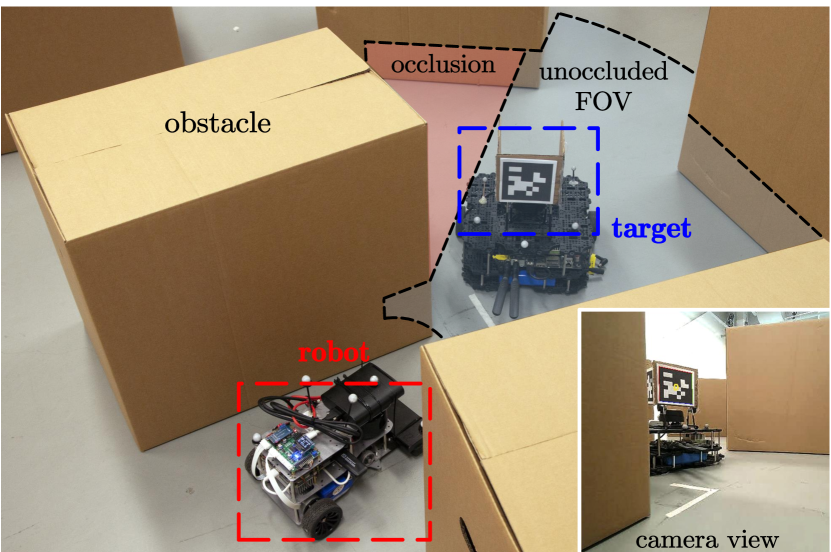
Figure 1: Illustration of visibility-aware tracking. The robot is equipped with an onboard sensor and is tasked with planning its trajectory to track a moving target in a cluttered environment while maintaining continual detection of the target.

Obstacle occlusion presents another challenge in target tracking. Such occlusion can be geometrically characterized, i.e., when a target is occluded by an obstacle, the line segment connecting the target and the robot, namely the line of sight (LOS), intersects with the obstacle. Following this line of thought, previous works have modeled obstacles as spheres and applied geometric distance costs in either the world frame [11] or the camera frame [10] to avoid occlusion. However, using spheres to envelop obstacles with varying shapes may lead to a conservative occlusion avoidance strategy. To overcome this limitation, researchers have proposed constructing a Euclidean Signed Distance Field (ESDF) to compute the occlusion cost for arbitrary obstacle shapes [12, 7]. Nevertheless, this method requires the offline computation of the ESDF to reduce the online computational burden hence rendering it ineffective in dynamic environments.

System uncertainty arising from imperfect system models and process noise can also degrade state estimation and trajectory planning in visibility-aware tracking tasks. Belief space planning [13] provides a systematic approach for handling such uncertainty by formulating a stochastic optimization problem to generate visibility maintenance trajectories, and the key step lies in the evaluation of predictive target visibility. A commonly employed method for predicting visibility is to evaluate the probability of detection (POD) by integrating predictive target probability density function (PDF) over the anticipated unoccluded FOV area [14, 15]. However, calculation of this integration can be either computationally burdensome when conducted over continuous state spaces [15] or inaccurate due to discretization error when transformed into the sum of probability mass over a grid detectable region [14]. Another approach is to directly determine target visibility based on the mean positions of the predicted target and the planned FOV [5, 6]. Despite the computational efficiency of this approach, such maximum-a-posteriori (MAP) estimation only considers mean positions, neglecting predictive target uncertainty during robot trajectory planning.

To overcome those limitations, our work proposes a model predictive control (MPC)-based non-myopic trajectory planner for mobile target tracking in cluttered environments. The proposed framework systematically considers limited FOV, obstacle occlusion, and state uncertainty during tracking, which is less investigated in current literature. The main contributions can be summarized as follows:

• We propose the concept of belief-space probability of detection (BPOD) that depends on both robot and target belief states to function as a measure of predicted visibility. We then develop an Extended Kalman Filter (EKF) variant that incorporates BPOD into target state prediction to take into account stochastic visibility in the MPC predictive horizon, which overcomes the deficiency of MAP estimation.

• We present a unified representation for both the BPOD and the collision risk as the probabilities of stochastic SDF satisfaction (PoSSDF) via the use of signed distance functions (SDFs), and develop a paradigm to efficiently calculate the PoSSDFs by linearizing the SDF around the mean values of robot and target distributions.

• We propose a real-time trajectory planner for visibility-aware target tracking in cluttered environments based on sequential convex programming (SCP). In particular, we propose a two-stage strategy for calculating SDF in SCP to accelerate the planner, reaching a computational speed of $10Hz$. Simulations and real-world experiments demonstrate that our method enables the robot to track a moving target in cluttered environments at high success rates and visible rates.

The remainder of the article is organized as follows. Sec. II formulates the target tracking problem. Sec. III defines BPOD and proposes a variant of EKF covariance update formulation to tackle uncertain visibility in the predictive horizon. Sec. IV approximates BPOD and collision risk by SDF linearization and proposes an SCP framework with the two-stage strategy for online trajectory planning. Simulations and real-world experiments are presented in Secs. V and VI, respectively. Sec. VII presents conclusions and future outlooks.

II Formulation of Target Tracking

II-A Motion Models and Obstacle Modeling

This work considers a discrete-time unicycle model as the robot dynamics:

$$\small\mathbf{z}^{r}_{k+1}=\mathbf{f}^{r}(\mathbf{z}^{r}_{k},\mathbf{u}^{r}_{k})+\mathbf{\mathbf{w}}^{r},\mathbf{\mathbf{w}}^{r}\sim\mathcal{N}(\mathbf{0},\mathbf{R}^{r}),$$ (1)

where

$$\small\mathbf{f}^{r}(\mathbf{z}^{r}_{k},\mathbf{u}^{r}_{k})=\mathbf{z}^{r}_{k}+[v_{k}^{r}\cos\theta_{k}^{r},\,v_{k}^{r}\sin\theta_{k}^{r},\,\omega_{k}^{r},\,a_{k}^{r}]^{T}\cdot\Delta t,$$

with $\Delta t$ representing the sampling interval. The robot state $\mathbf{z}^{r}_{k}=[{\mathbf{x}^{r}_{k}}^{T},\theta_{k}^{r},v_{k}^{r}]^{T}\in\mathbb{R}^{4}$ contains position ${\mathbf{x}^{r}_{k}}\in\mathbb{R}^{2}$, orientation $\theta_{k}^{r}\in(-\pi,\pi]$, and velocity $v_{k}^{r}\in\mathbb{R}_{+}$, where the subscript $k$ means time step. The control input $\mathbf{u}^{r}_{k}=[\omega_{k}^{r},a_{k}^{r}]^{T}\in\mathbb{R}^{2}$ is composed of angular velocity $\omega_{k}^{r}\in\mathbb{R}$ and acceleration $a_{k}^{r}\in\mathbb{R}$. The process noise $\mathbf{w}^{r}$ follows a Gaussian distribution with a zero mean and covariance matrix $\mathbf{R}^{r}$. We assume the robot’s current state is known.

The target motion model is defined as

$$\small\mathbf{z}^{t}_{k+1}=\mathbf{f}^{t}(\mathbf{z}^{t}_{k},\mathbf{u}^{t}_{k})+\mathbf{w}^{t},\ \ \mathbf{w}^{t}\sim\mathcal{N}(\mathbf{0},\mathbf{R}^{t}),$$ (2)

where $\mathbf{z}^{t}_{k}\in\mathbb{R}^{d_{t}}$ denotes the target state with dimension $d_{t}$, $\mathbf{u}^{t}_{k}$ represents the target control input. We define the elements in $\mathbf{z}^{t}_{k}$ that correspond to the target position as $\mathbf{x}^{t}_{k}\in\mathbb{R}^{2}$. The target motion function $\mathbf{f}^{t}$ will be specified in Sec. V, and the motion noise $\mathbf{w}^{t}$ follows a Gaussian distribution with a zero mean and covariance matrix $\mathbf{R}^{t}$. Target state $\mathbf{z}^{t}_{k}$ remains unknown and needs to be estimated.

This work considers a known continuous map $\mathcal{M}\in\mathbb{R}^{2}$ with convex obstacles represented as point sets $\mathcal{O}_{i}\subset\mathcal{M},i=1,2,\cdots,N_{o}$, where $N_{o}$ denotes the number of obstacles. Note that the proposed approach can also address nonconvex obstacles by dividing them into multiple convex ones.

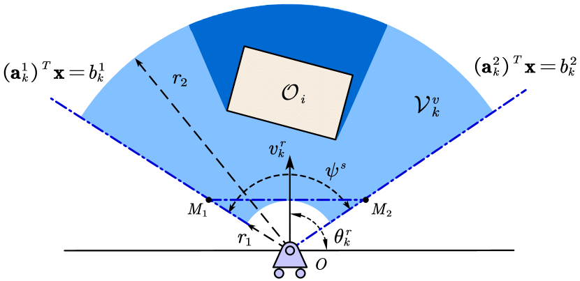
Figure 2: Illustration of FOV and occlusion. The polygon $\mathcal{O}_{i}$ represents an obstacle, and the light blue area $\mathcal{V}^{v}_{k}$ represents the non-occluded part of the FOV. Point $O$ denotes the robot position, and line $M_{1}M_{2}$ is tangent to the inner arc and perpendicular to the robot’s orientation $\theta_{k}^{r}$.

II-B Sensor Model

The robot’s sensor FOV is modeled as an annular sector:

$$\small\mathcal{V}_{k}=\{\mathbf{x}|\mathbf{a}^{i}_{k}\cdot\mathbf{x}\leq b^{i}_{k},r_{1}\leq\|\mathbf{x}-\mathbf{x}^{r}_{k}\|\leq r_{2},i=1,2\},$$

where $\|\cdot\|$ means the Euclidean norm, $\mathbf{a}^{1}_{k},\mathbf{a}^{2}_{k}\in\mathbb{R}^{2},b^{1}_{k},b^{2}_{k}\in\mathbb{R}$ form the two linear boundaries that limit the maximum detection angle $\psi^{s}$, and $r_{1},r_{2}\in\mathbb{R_{+}}$ constrain the detection range. The FOV is illustrated in Fig. 2.

The sensor model described in this work considers intermittent measurements due to potential target loss caused by the limited FOV and occlusions, which is defined as

$$\small\mathbf{y}_{k}=\left\{\begin{array}[]{c}\mathbf{f}^{s}(\mathbf{z}_{k}^{t},\mathbf{z}_{k}^{r})+\mathbf{w}^{s},\ \mathbf{x}^{t}_{k}\in\mathcal{V}_{k}^{v}\\ \varnothing,\qquad\quad\qquad\ \ \ \ \mathbf{x}^{t}_{k}\notin\mathcal{V}_{k}^{v}\end{array}\right.,$$ (3)

where $\mathbf{y}_{k}\in\mathbb{R}^{d_{m}}$ is the measurement with dimension $d_{m}$ and the measurement function $\mathbf{f}^{s}$ will be specified in Sec. V. The sensor noise $\mathbf{w}^{s}$ follows a Gaussian distribution with a zero mean and covariance matrix $\mathbf{R}^{s}$. Here $\mathcal{V}^{v}_{k}$ is a subset of $\mathcal{V}_{k}$ that is not occluded by any obstacles, as illustrated in Fig. 2.

II-C Extended Kalman Filter with Intermittent Measurements

The robot needs accurately estimate the target state based on sensor measurements to make informed tracking behavior. To account for the system nonlinearity and possible target loss, we develop a variant of EKF for target state estimation to take intermittent measurements into account, inspired by [16]. The filtering procedure can be summarized as follows.

Prediction. Predict the prior PDF using target kinematics,

$$\small\hat{\mathbf{z}}^{t}_{k|k-1} =\mathbf{f}^{t}(\hat{\mathbf{z}}^{t}_{k-1|k-1},\mathbf{u}^{t}_{k-1}),$$ (4a)

$$\mathbf{P}_{k|k-1} =\mathbf{A}^{t}_{k-1}\mathbf{P}_{k-1|k-1}(\mathbf{A}^{t}_{k-1})^{T}+\mathbf{R}^{t},$$ (4b)

where $\hat{\mathbf{z}}^{t}_{k-1|k-1}$ and $\mathbf{P}_{k-1|k-1}$ represent the mean and covariance of the estimate of $\mathbf{z}^{t}_{k-1}$, and $\mathbf{A}^{t}_{k-1}=\nabla_{\mathbf{z}^{t}}\mathbf{f}^{t}(\mathbf{z}^{t},\mathbf{u}^{t}_{k-1})|_{\mathbf{z}^{t}=\hat{\mathbf{z}}^{t}_{k-1|k-1}}$ is the Jacobi matrix of the target kinematic model.

Update. Use current measurements to update target PDF,

$$\small\mathbf{K}_{k} =\mathbf{P}_{k|k-1}\mathbf{C}_{k}^{T}(\mathbf{C}_{k}\mathbf{P}_{k|k-1}{\mathbf{C}^{T}_{k}}+\mathbf{R}^{s})^{-1},$$ (5a)

$$\hat{\mathbf{z}}^{t}_{k|k} =\hat{\mathbf{z}}^{t}_{k|k-1}+\mu_{k}\mathbf{K}_{k}(\mathbf{y}_{k}-\mathbf{f}^{s}(\hat{\mathbf{z}}_{k|k-1}^{t},\mathbf{z}_{k}^{r})),$$ (5b)

$$\mathbf{P}_{k|k} =\mathbf{P}_{k|k-1}-\mu_{k}\mathbf{K}_{k}\mathbf{C}_{k}\mathbf{P}_{k|k-1},$$ (5c)

where $\mathbf{C}_{k}=\nabla_{\mathbf{z}^{t}}\mathbf{f}^{s}(\mathbf{z}^{t},\mathbf{z}^{r}_{k})|_{\mathbf{z}^{t}=\hat{\mathbf{z}}^{t}_{k|k-1}}$ is the Jacobi matrix of the measurement model, and $\mu_{k}$ is the detection variable (DV) that determines whether the target is detected, calculated as

$$\small\mu_{k}=\left\{\begin{array}[]{c}1,\ \ \ \ \mathbf{y}_{k}\neq\varnothing\\ 0,\ \ \ \ \mathbf{y}_{k}=\varnothing\\ \end{array}\right..$$ (6)

II-D MPC Formulation for Trajectory Planning

The trajectory planner is formulated as an MPC problem:

$$\small\min_{\mathbf{u}^{r}_{k:k+N-1}} J(\mathbf{b}^{r}_{k+1:k+N},\mathbf{b}^{t}_{k+1:k+N})$$ (7a)

$$s.t.\ \ \ \mathbf{b}^{t}_{k+i}=\mathbf{g}^{t}(\mathbf{b}^{t}_{k+i-1},\mathbf{b}^{r}_{k+i-1}),$$ (7b)

$$\mathbf{b}^{r}_{k+i}=\mathbf{g}^{r}(\mathbf{b}^{r}_{k+i-1},\mathbf{u}^{r}_{k+i-1}),$$ (7c)

$$\mathbf{b}^{r}_{k+i}\in\mathcal{B}^{r},\mathbf{b}_{k+i}^{t}\in\mathcal{B}^{t},\mathbf{u}^{r}_{k+i-1}\in\mathcal{U},$$ (7d)

$$\mathbf{f}^{o}(\mathbf{b}^{r}_{k+i},\mathcal{O}_{j})<0,$$ (7e)

$$j=1,2,\cdots,N_{o},\ i=1,\cdots,N,$$

where $N$ stands for MPC planning horizon. The target belief state $\mathbf{b}^{t}_{k}=[\hat{\mathbf{z}}_{k|k}^{t},\mathbf{P}_{k|k}]$ encodes the probability distribution of the estimated target state. Due to the existence of process noise, the robot state is stochastic in the predictive horizon. Therefore, we define the robot belief state $\mathbf{b}^{r}_{k}=[{\hat{\mathbf{z}}^{r}_{k}},\mathbf{Q}_{k}]$ to encode mean value $\hat{\mathbf{z}}^{r}_{k}$ and covariance matrix $\mathbf{Q}_{k}$ of robot state. The sets $\mathcal{B}^{r},\ \mathcal{B}^{t}$ and $\mathcal{U}$ are the feasible sets of robot belief state, target belief state and robot control input, respectively. The functions $\mathbf{g}^{r}(\cdot)$ and $\mathbf{g}^{t}(\cdot)$ denote belief prediction procedures, which will be described in detail in the next section. The objective function Eq. 7a and the collision avoidance constraint Eq. 7e will be further elaborated in Secs. III and IV.

III Belief-Space Probability of Detection-Based State Prediction

III-A Probabilistic State Prediction in Predictive Horizon

We employ two different EKF-based approaches for the state prediction of the robot and target. Note that the lack of observation needs to be properly addressed, which differs from the estimation process Eqs. 4a, 4b, 5a, 5b and 5c.

Robot state prediction. Like Eqs. 4a and 4b, we use the prediction step of EKF to predict the robot state in the predictive horizon. Specifically, Eq. 7c is specified as

$$\small\hat{\mathbf{z}}_{k+i}^{r} =\mathbf{f}^{r}(\hat{\mathbf{z}}^{r}_{k+i-1},\mathbf{u}_{k+i-1}^{r}),$$ (8a)

$$\mathbf{Q}_{k+i} =\mathbf{A}^{r}_{k+i-1}\mathbf{Q}_{k+i-1}(\mathbf{A}^{r}_{k+i-1})^{T}+\mathbf{R}^{r},$$ (8b)

where $\mathbf{A}^{r}_{k+i-1}=\nabla_{\mathbf{z}^{r}}\mathbf{f}^{r}(\mathbf{z}^{r},\mathbf{u}^{r}_{k+i-1})|_{\mathbf{z}^{r}=\hat{\mathbf{z}}^{r}_{k+i-1}}$ is the Jacobi matrix of the robot kinematic model.

Target state prediction. The target mean $\hat{\mathbf{z}}_{k|k}^{t}$ is simply propagated using its kinematics due to unknown predictive measurements, and the covariance $\mathbf{P}_{k|k-1}$ is predicted by using Eq. 4b. However, the target visibility is uncertain in the predictive horizon, making it difficult to predict DV and update the covariance following Eqs. 5a and 5c. To deal with this difficulty, we propose the concept of BPOD to denote the probability that the target is detected, defined as

$$\small\gamma_{k} =Pr(\mathbf{y}_{k}\neq\varnothing|\mathbf{b}^{r}_{k},\mathbf{b}^{t}_{k|k-1}),$$ (9)

where $\mathbf{b}^{t}_{k|k-1}=[\hat{\mathbf{z}}_{k|k-1}^{t},\mathbf{P}_{k|k-1}]$. Compared to traditional PODs that are either determined by the ground truth of robot and target positions [17] or only depend on the predictive target distribution under deterministic robot states [14, 15], BPOD is conditioned on the belief states of both the robot and the target, which provides a more precise measurement of visibility under stochastic robot and target states. Next, we will incorporate the BPOD into EKF and constitute the stochastic counterpart of Eq. 5c to tackle uncertain predictive visibility.

Recall that the DV is determined by the relative pose of the robot and the target, and thus can be reformulated as

$$\small\mu_{k} =Pr(\mathbf{y}_{k}\neq\varnothing|\mathbf{z}^{r}_{k},\mathbf{z}^{t}_{k}).$$ (10)

Denote $\mathbb{E}_{z|b}(\cdot)$ as the expectation operator with respect to $\mathbf{z}^{t}_{k}$ and $\mathbf{z}^{r}_{k}$ conditioned on $\mathbf{b}^{t}_{k|k-1}$ and $\mathbf{b}^{r}_{k}$, we can adopt the total probability rule (TPR) and derive $\gamma_{k}=\mathbb{E}_{z|b}(\mu_{k})$. Combining Eq. 10 and the EKF procedures, we can find that $\mathbf{P}_{k|k}$ in Eq. 5c is conditioned on $\mathbf{z}^{r}_{k}$ and $\mathbf{z}^{t}_{k}$. Note that accurate estimates of the robot and target states are not available in the predictive horizon. Therefore, the posterior covariance $\tilde{\mathbf{P}}_{k|k}$ in predictive horizon only depends on the predictive robot and target beliefs, and thus can be formulated as the conditional expectation of $\mathbf{P}_{k|k}$, i.e., $\tilde{\mathbf{P}}_{k|k}=\mathbb{E}_{z|b}(\mathbf{P}_{k|k})$ according to TPR. Following this idea, we propose a visibility-aware covariance update scheme, which is formulated as follows:

$$\small\tilde{\mathbf{P}}_{k|k} =\mathbb{E}_{z|b}(\mathbf{P}_{k|k})$$ (11a)

$$\approx\mathbb{E}_{z|b}(\mathbf{P}_{k|k-1}-\mu_{k}\tilde{\mathbf{K}}_{k}\tilde{\mathbf{C}}_{k}\mathbf{P}_{k|k-1})$$ (11b)

$$=\mathbf{P}_{k|k-1}-\mathbb{E}_{z|b}(\mu_{k})\tilde{\mathbf{K}}_{k}\tilde{\mathbf{C}}_{k}\mathbf{P}_{k|k-1}$$ (11c)

$$=\mathbf{P}_{k|k-1}-\gamma_{k}\tilde{\mathbf{K}}_{k}\tilde{\mathbf{C}}_{k}\mathbf{P}_{k|k-1},$$ (11d)

where covariance $\mathbf{P}_{k|k-1}$ and $\mathbf{P}_{k|k}$ are defined in Eqs. 4b and 5c, respectively, and $\tilde{\mathbf{C}}_{k}$, $\tilde{\mathbf{K}}_{k}$ denote the approximate measurement Jacobi matrix and Kalman gain, respectively. To simplify the computation, we approximate the measurement Jacobi matrix as being equal to the one determined by the mean value of robot belief $\hat{\mathbf{z}}_{k}^{r}$, i.e., $\tilde{\mathbf{C}}_{k}=\nabla_{\mathbf{z}^{t}}\mathbf{f}^{s}(\mathbf{z}^{t},\hat{\mathbf{z}}^{r}_{k})|_{\mathbf{z}^{t}=\hat{\mathbf{z}}^{t}_{k|k-1}}$, and calculate the Kalman gain $\tilde{\mathbf{K}}_{k}$ from Eq. 5a by replacing $\mathbf{C}_{k}$ with $\tilde{\mathbf{C}}_{k}$, which yields Eq. 11b. Eq. 11c is derived by the independency of $\tilde{\mathbf{K}}_{k}$ and $\tilde{\mathbf{C}}_{k}$ from $\mathbf{z}^{t}_{k}$ and $\mathbf{z}^{r}_{k}$.

Eq. 11d is a probabilistic extension of Eq. 5c that allows us to update the target covariance in Eq. 7b using only the predicted beliefs of the robot and target. Intuitively speaking, smaller BPOD means a lower probability of the target to be observed, which in turn corresponds to higher predictive uncertainty of the target (Fig. 3). To further justify our proposed new formulation for covariance update, we can prove that a larger BPOD indeed leads to reduced uncertainty.

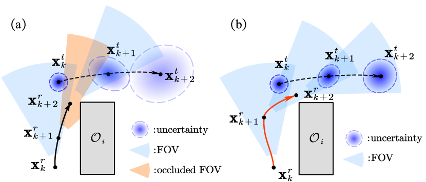
Figure 3: Relationship between BPOD and predictive uncertainty of target. In contrast to the black trajectory in (a) that leads to FOV being partially blocked, if the robot follows the red trajectory in (b), it is expected to keep better visibility of the target due to unoccluded sight and better coverage of target PDF by FOV. Target uncertainty is consequently smaller in (b).

Proposition 1 (Monotonic Decrease of Covariance Determinant with Respect to Increasing BPOD)

Define the function

$$\small f(\gamma)=|\mathbf{P}_{k|k-1}-\gamma\tilde{\mathbf{K}}_{k}\tilde{\mathbf{C}}_{k}\mathbf{P}_{k|k-1}|,\gamma\in[0,1],$$

where $|\cdot|$ is the determinant. Then following inequality holds,

$$f(\gamma_{1})\geq f(\gamma_{2}),\ \forall\gamma_{1}\leq\gamma_{2}.$$

Proof:

For convenience, we define

$$\mathbf{\Psi}=\tilde{\mathbf{K}}_{k}\tilde{\mathbf{C}}_{k}\mathbf{P}_{k|k-1},\quad\mathbf{\Phi}=\mathbf{P}_{k|k-1}-\gamma_{2}\mathbf{\mathbf{\Psi}}.$$

Following inequalities hold for EKF given the definitions of $\mathbf{\Psi}$ and $\mathbf{\Phi}$ in Kalman Filter[18],

$$\mathbf{\mathbf{\Psi}}\succeq 0,\,\,\mathbf{P}_{k|k-1}-\mathbf{\mathbf{\Psi}}\succeq 0,$$ (12)

where “$\succeq$" denotes semi-definiteness.

Using Eq. 12 and the constraint that $\gamma_{2}\leq 1$, it is obvious that $\mathbf{\Phi}$ is also semi-definite. Then we can derive that

$$\leavevmode\resizebox{394.59578pt}{}{$|\mathbf{P}_{k|k-1}-\gamma_{1}\mathbf{\mathbf{\Psi}}|=|\mathbf{\Phi}+(\gamma_{2}-\gamma_{1})\mathbf{\mathbf{\Psi}}|\geq|\mathbf{\Phi}|+|(\gamma_{2}-\gamma_{1})\mathbf{\mathbf{\Psi}}|\geq|\mathbf{\Phi}|$},$$

where the first inequality is derived by the superadditivity property of determinant for semi-definite matrices [19]. ∎

In information theory, entropy is widely used as a measure of uncertainty. Due to the Gaussian assumption of EKF, the entropy of target belief state can be formulated as follows [20],

$$\small\mathcal{H}(\mathbf{b}^{t}_{k})=\frac{d_{t}}{2}(\ln(2\pi)+1)+\frac{1}{2}\ln|\mathbf{P}_{k|k}|.$$ (13)

Combining 1, we can conclude that higher BPOD results in smaller target uncertainty in the sense of entropy, which motivates the use of the following objective functions.

III-B Objective Function

There are two mainstream choices of the objective function for target tracking, i.e., to minimize target uncertainty[5, 15], or to maximize the predictive visibility of the target[14]. We correspondingly formulate two objectives as

$$\small J_{1}=\sum_{i=1}^{N}\mathcal{H}(\mathbf{b}^{t}_{k+i}),\ \ J_{2}=-\sum_{i=1}^{N}\gamma_{k+i},$$ (14)

where $J_{1}$ is the cumulative entropy and $J_{2}$ is the negation of cumulative BPOD. With the help of 1 and Eq. 13, we show that these two objectives are compatible, such that minimizing $J_{2}$ will simultaneously decrease $J_{1}$. Both two objective functions are tested in our simulations, as will be presented in Sec. V, and are shown to achieve similar performance in effectively keeping the target visible and decreasing estimation error.

IV Signed Distance Function-Based Online Trajectory Planning

IV-A Unified Expression of Visibility and Collision Risk

Limited FOV and occlusion are two major factors that influence visibility. Following this idea, we define two corresponding probabilities to compute Eq. 9.

Target and FOV. We define the probability of the target being within the FOV area as:

$$\gamma^{tf}_{k}=Pr(\mathbf{x}^{t}_{k}\in\mathcal{V}_{k}|\mathbf{b}_{k}^{r},\mathbf{b}_{k|k-1}^{t}).$$ (15)

LOS and Obstacle. Likewise, we express the probability that the target is not occluded by obstacle $i$ as:

$$\gamma^{lo}_{k,i}=Pr(\mathcal{L}_{k}\bigcap\mathcal{O}_{i}=\varnothing|\mathbf{b}_{k}^{r},\mathbf{b}_{k|k-1}^{t}),$$ (16)

where $\mathcal{L}_{k}$ is the line segment between $\mathbf{x}^{t}_{k}$ and $\mathbf{x}^{r}_{k}$. Reasonably, we can assume that all variables in $\{\gamma^{tf}_{k},\gamma^{lo}_{k,1},\cdots,\gamma^{lo}_{k,N_{o}}\}$ are mutually independent. Then the BPOD can be factorized as

$$\gamma_{k}=\gamma^{tf}_{k}\prod_{i=1}^{N_{o}}\gamma^{lo}_{k,i}.$$ (17)

To avoid overly conservative trajectory while ensuring safety, we define chance-constrained[21] collision avoidance conditions that bound the collision risk below a user-defined threshold $\delta^{s}\in\mathbb{R}$. The probability of collision between the robot and obstacle $i$ at time $k$ is defined as

$$\small\gamma^{ro}_{k,i}=Pr(\mathbf{x}^{r}_{k}\in\mathcal{O}_{i}|\mathbf{b}_{k}^{r},\mathbf{b}_{k|k-1}^{t}).$$ (18)

Eq. 7e is then specified as the chance constraints, i.e.,

$$\gamma^{ro}_{k+i,j}<\delta^{s}_{k+i,j}.$$ (19)

In order to solve the MPC problem Eq. 7, it is crucial to efficiently compute $\gamma^{tf}$, $\gamma^{lo}$, and $\gamma^{ro}$ as specified in Eqs. 15, 18 and 16. A main contribution of this work is to represent and compute the BPOD and chance-constrained collision risk in a unified manner that significantly reduces the computational burden of solving the MPC problem, which will be described in the next subsection. For clarity, we define the set $\Gamma_{k}=\{\gamma^{tf}_{k},\gamma^{lo}_{k,i},\gamma^{ro}_{k,i},i=1,\cdots,N_{o}\}$.

1 Input: two rigid bodies: $\mathcal{A}_{1}(\mathbf{x}),\mathcal{A}_{2}(\mathbf{x})$, $\mathbf{x}\sim\mathcal{N}(\hat{\mathbf{x}},\Sigma)$,

2         SDF parameters $\hat{p}^{L}_{1},\hat{p}^{L}_{2},\hat{\mathbf{n}}$

3

4Output: $p=Pr(sd(\mathcal{A}_{1}(\mathbf{x}),\mathcal{A}_{2}(\mathbf{x}))\leq 0)$

5

6     $\mathbf{p}_{i}(\mathbf{x})\leftarrow\mathbf{R}_{i}(\mathbf{x})\hat{p}_{i}^{L}+\mathbf{p}^{c}_{i}(\mathbf{x}),i=1,2$

7

8     $sd(\mathbf{x})\leftarrow\hat{\mathbf{n}}^{T}(\mathbf{p}_{1}(\mathbf{x})-\mathbf{p}_{2}(\mathbf{x}))$

9      $sd_{L}(\mathbf{x})\leftarrow sd(\hat{\mathbf{x}})+\nabla_{\mathbf{x}}sd(\mathbf{x})|_{\mathbf{x}=\hat{\mathbf{x}}}(\mathbf{x}-\hat{\mathbf{x}})$

10

     $p\leftarrow\text{Calculate }Pr(sd_{L}(\mathbf{x})\leq 0)$

Algorithm 1 Calculation of PoSSDF

IV-B Approximating $\Gamma_{k}$ with Linearized SDF

The SDF quantifies the distance between two shapes. Specifically, the SDF of two sets $\mathcal{A},\mathcal{B}\subset\mathbb{R}^{2}$ is formulated as the minimum translation distance required to separate or intersect each other, i.e.,

$$\small sd\left(\mathcal{A},\mathcal{B}\right)=\left\{\begin{array}[]{c}\inf\left\{\left\|\mathbf{v}\right\|\,|\left(\mathbf{v}+\mathcal{A}\right)\bigcap{\mathcal{B}\neq\varnothing}\right\},\mathcal{A}\bigcap{\mathcal{B}}=\varnothing\\ \inf\left\{\left\|\mathbf{v}\right\|\,|\left(\mathbf{v}+\mathcal{A}\right)\bigcap{\mathcal{B}=\varnothing}\right\},\mathcal{A}\bigcap{\mathcal{B}}\neq\varnothing\\ \end{array}\right.,$$

where $\mathbf{v}\in\mathbb{R}^{2}$ is the translation vector. Using SDF, we can equivalently reformulate Eqs. 15, 16 and 18 as follows,

$$\small\gamma^{tf}_{k} =Pr(sd(\mathbf{x}^{t}_{k},\mathcal{V}_{k})\leq 0|\mathbf{b}_{k}^{r},\mathbf{b}_{k|k-1}^{t}),$$ (20)

$$\gamma^{lo}_{k,i} =Pr(sd(\mathcal{L}_{k},\mathcal{O}_{i})\geq 0|\mathbf{b}_{k}^{r},\mathbf{b}_{k|k-1}^{t}),$$ (21)

$$\gamma^{ro}_{k,i} =Pr(sd(\mathbf{x}^{r}_{k},\mathcal{O}_{i})\leq 0|\mathbf{b}_{k}^{r},\mathbf{b}_{k|k-1}^{t}).$$ (22)

Note that Eqs. 20, 21 and 22 are all PoSSDFs because $\mathbf{x}^{t}_{k},\mathbf{x}^{r}_{k},\mathcal{L}_{k}$ and $\mathcal{V}_{k}$ are all random variables given robot and target beliefs. These probabilities can be evaluated using Monte-Carlo simulation, but at the cost of heavy computational burden. Inspired by [22], we propose a computationally efficient paradigm to evaluate PoSSDF using a linearized SDF expression, as described in Alg. 1.

The inputs of Alg. 1 include two rigid bodies $\mathcal{A}_{1},\mathcal{A}_{2}\subset\mathbb{R}^{2}$, whose poses are determined by an arbitrary random Gaussian variable $\mathbf{x}$ with dimension $d_{x}$. This algorithm also needs to precalculate the signed distance $\hat{d}\in\mathbb{R}$ between $\mathcal{A}_{1}(\hat{\mathbf{x}})$ and $\mathcal{A}_{2}(\hat{\mathbf{x}})$, along with the closest points from each set, $\hat{\mathbf{p}}_{1}\in\mathcal{A}_{1}(\hat{\mathbf{x}}),\hat{\mathbf{p}}_{2}\in\mathcal{A}_{2}(\hat{\mathbf{x}})$, as illustrated in Fig. 4(a). This operation can be efficiently carried out by using one of the two popular algorithms: Gilbert–Johnson–Keerthi (GJK) algorithm [23] for minimum distance, and Expanding Polytope Algorithm (EPA)[24] for penetration depth. Then we obtain the SDF parameters including the contact normal $\hat{\mathbf{n}}=sgn(\hat{d})\cdot(\hat{\mathbf{p}}_{1}-\hat{\mathbf{p}}_{2})/\|\hat{\mathbf{p}}_{1}-\hat{\mathbf{p}}_{2}\|$, and the local coordinates of $\hat{\mathbf{p}}_{1}$ and $\hat{\mathbf{p}}_{2}$ relative to $\mathcal{A}_{1}(\hat{\mathbf{x}})$ and $\mathcal{A}_{2}(\hat{\mathbf{x}})$ respectively, noted as $\hat{p}^{L}_{1}$ and $\hat{p}^{L}_{2}$. Alg. 1 provides an analytical approximation of the closest points $\mathbf{p}_{1}(\mathbf{x})$ and $\mathbf{p}_{2}(\mathbf{x})$ in the world frame. Here we assume that the local coordinates of $\mathbf{p}_{1}(\mathbf{x})$ and $\mathbf{p}_{2}(\mathbf{x})$, relative to $\mathcal{A}_{1}(\mathbf{x})$ and $\mathcal{A}_{2}(\mathbf{x})$ respectively, are fixed and equal to $\hat{p}^{L}_{1}$ and $\hat{p}^{L}_{2}$. The approximate closest point $\mathbf{p}_{i}(\mathbf{x})$ in the world frame can then be obtained by using $\mathbf{R}_{i}(\mathbf{x})$, the rotation matrix of $\mathcal{A}_{i}(\mathbf{x})$, and $\mathbf{p}_{i}^{c}(\mathbf{x})$, the origin of the local coordinate system attached to $\mathcal{A}_{i}(\mathbf{x})$. In Alg. 1, the SDF between $\mathcal{A}_{1}(\mathbf{x})$ and $\mathcal{A}_{2}(\mathbf{x})$ is approximated by projecting the distance between $\mathbf{p}_{1}(\mathbf{x})$ and $\mathbf{p}_{2}(\mathbf{x})$ onto the contact normal $\hat{\mathbf{n}}$. Fig. 4(a) illustrates the SDF approximation in Algs. 1 and 1. In Algs. 1 and 1, we linearize the SDF around the Gaussian mean and analytically calculate the PoSSDF using the fact that the probability of a linear inequality for a Gaussian variable can be explicitly expressed as follows[25],

$$Pr(\mathbf{a}^{T}\cdot\mathbf{x}\leq b)=\frac{1}{2}(1-\text{erf}(\frac{\mathbf{a}^{T}\cdot\hat{\mathbf{x}}-b}{\sqrt{2\mathbf{a}^{T}\Sigma\mathbf{a}}})),$$

where $\text{erf}(\cdot)$ represents the Gauss error function, and $\mathbf{a}\in\mathbb{R}^{d_{x}},b\in\mathbb{R}$ form the linear constraint of $\mathbf{x}$.

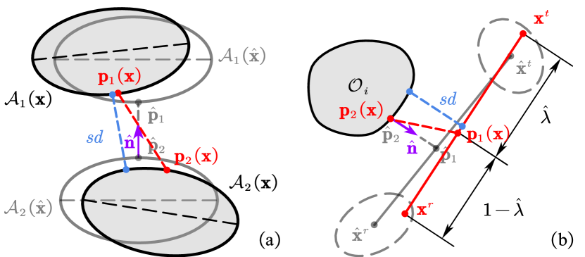
Figure 4: Illustration of SDF approximation in Alg. 1. The blue segment represents the true SDF value of two sets $\mathcal{A}_{1}(\mathbf{x})$ and $\mathcal{A}_{2}(\mathbf{x})$, while the approximate SDF is calculated by projecting $\mathbf{p}_{1}(\mathbf{x})-\mathbf{p}_{2}(\mathbf{x})$ (the red dashed segment) to $\hat{\mathbf{n}}$ (the purple vector). (a) A general case. (b) Application of Alg. 1 to calculate $\gamma^{lo}$ with the dashed ellipses denoting the uncertainties of the robot and the target.

Alg. 1 provides a general procedure to calculate PoSSDF. Denote $\mathbf{x}=\left[{\mathbf{z}_{k}^{r}}^{T},{\mathbf{z}_{k}^{t}}^{T}\right]^{T}$, we can make the following adjustments and apply Alg. 1 to efficiently calculate $\Gamma_{k}$. First, feeding $\mathcal{V}_{k}$ into Alg. 1 is error-prone for $\gamma^{tf}$ calculation because $\mathcal{V}_{k}$ is nonconvex. Therefore, we convexify the FOV by excluding the area in $\Delta M_{1}M_{2}O$ (see Fig. 2 for detail). Second, to take the variable length of the LOS $\mathcal{L}_{k}(\mathbf{x})$ into account when calculating $\gamma^{lo}$, we precalculate the separative ratio $\hat{\lambda}$ of $\mathcal{L}_{k}(\hat{\mathbf{x}})$ before carrying out Alg. 1, which is formulated as

$$\small\hat{\lambda}=\|\hat{\mathbf{p}}_{1}-\hat{\mathbf{x}}^{t}_{k}\|/\|\hat{\mathbf{x}}^{r}_{k}-\hat{\mathbf{x}}^{t}_{k}\|,$$

where $\hat{\mathbf{p}}_{1}$ is the nearest point on $\mathcal{L}_{k}(\hat{\mathbf{x}})$. We then replace the SDF parameter $\hat{p}_{1}^{L}$ with $\hat{\lambda}$ and reformulate the approximated nearest point (Alg. 1) on $\mathcal{L}_{k}(\mathbf{x})$ in the world frame as

$$\small\mathbf{p}_{1}(\mathbf{x})=\hat{\lambda}\mathbf{x}^{r}_{k}(\mathbf{x})+(1-\hat{\lambda})\mathbf{x}^{t}_{k}(\mathbf{x}).\\$$

This adjustment for calculating $\gamma^{lo}$ is illustrated in Fig. 4(b).

Note that Eq. 19 is not violated even though we alternatively bound the collision probability approximated by Alg. 1 below threshold $\delta^{s}$. This is because in Alg. 1, the obstacle is expanded to a half space with the closest point on its boundary and $\hat{\mathbf{n}}$ being its normal vector. This process overestimates $\gamma^{ro}$ thus ensuring Eq. 19 to be strictly enforced.

IV-C Sequential Convex Optimization

After being specified in Secs. IV-A and IV-B, problem Eq. 7 can be solved using the SCP algorithm, where the nonlinear constraints are converted into $l_{1}$ penalty functions,

$$\small J_{m}=J+\eta(\sum_{i}|g^{n}_{i}|^{+}+\sum_{i}|h^{n}_{i}|).$$ (23)

Here $J$ denotes the objective function Eq. 7a, and $g_{i}^{n}$, $h_{i}^{n}$ represent the nonlinear inequality and equality constraints, respectively. Here $\eta$ is the penalty coefficient and $|x|^{+}=\max(x,0)$. The SCP consists of two loops: The outer loop progressively increases $\eta$ to drive the nonlinear constraint violation to zero, while in the inner loop, the trust region method is implemented to minimize the new objective function ${J}_{m}$. Interested readers can refer to [22] for details.

Directly adopting this framework turns out to be slow due to the frequent calls of GJK algorithms and EPA when calculating the gradient of Eq. 23. To overcome this limitation, we use a fixed SDF parameter set that encodes all the SDF parameters in the MPC horizon to calculate $\Gamma_{k+1:k+N}$ in the gradient, and update the SDF parameter set after obtaining a new solution. This two-stage strategy significantly speeds up the planner with minor accuracy loss, and is further described in the SCP-based trajectory planning framework presented in Alg. 2.

1 Parameters:

2      $\eta:\text{initial penalty coefficient}$

3      $d:\text{initial trust region size}$

4      $\beta:\text{increase ratio of the penalty coefficient}$

5      $\tau_{c},\tau_{p},\tau_{f}:\text{convergence tolerances}$

6 Output: $x^{\ast}=\mathbf{u}^{r}_{k:k+N-1}:\text{the optimal solution}$

7 $x_{0},\mathcal{C}_{0}\leftarrow$ Initialize the solution and SDF parameter set

8 while TRUE do

9       while TRUE do

10             $\nabla J_{x}\leftarrow$ Get the gradient of $J_{m}$ on $x_{0}$ using $\mathcal{C}_{0}$

11             $\tilde{J}(x,\eta,\mathcal{C}_{0})\leftarrow J_{m}(x_{0},\eta,\mathcal{C}_{0})+\nabla J_{x}\cdot(x-x_{0})$

12             $x^{\ast}\leftarrow\textbf{argmin}_{x}\tilde{J}(x,\eta,\mathcal{C}_{0})$ subject to trust region, linear constraints, and semidefinite constraints of covariance matrices.

13             $\mathcal{C}^{\ast}\leftarrow$ Update SDF parameter set from $x^{\ast}$

14             $d\leftarrow$ Update trust region size by improvement ratio $\frac{J_{m}(x_{0},\eta,\mathcal{C}_{0})-J_{m}(x^{\ast},\eta,\mathcal{C}^{\ast})}{J_{m}(x_{0},\eta,\mathcal{C}_{0})-\tilde{J}(x^{\ast},\eta,\mathcal{C}_{0})}$

15             $\textbf{If }\|x^{\ast}-x_{0}\|\leq\tau_{c}\textbf{ or }|\nabla J_{x}\cdot(x^{\ast}-x_{0})|\leq\tau_{f}\ \textbf{break}$

16             $x_{0}\leftarrow x^{\ast}$, $\mathcal{C}_{0}\leftarrow\mathcal{C}^{\ast}$ If trust region is expanded

17       end while

18      $\textbf{If}\sum_{i}|g^{n}_{i}(x^{\ast},\mathcal{C}^{\ast})|^{+}+\sum_{j}|h^{n}_{j}(x^{\ast},\mathcal{C}^{\ast})|\leq\tau_{p}\ \textbf{break}$

19       $\eta\leftarrow\beta\cdot\eta$

20 end while

Algorithm 2 Trajectory Planning in SCP Framework with Two-Stage Strategy for Efficient SDF Calculation

The variable $x_{0}$ is initialized with zero control inputs at the first step, and is extrapolated from its value at the previous step for all subsequent steps. This is followed by precalculating an SDF parameter set $\mathcal{C}_{0}$ at the mean value of the initial robot and target beliefs, which is propagated by $x_{0}$ (Alg. 2). Using a fixed $\mathcal{C}_{0}$, we can fastly obtain the gradient (Alg. 2) and linearize the objective function (Alg. 2). After solving the linearized problem, the SDF parameter set is updated (Alg. 2) and utilized to update the trust region size (Alg. 2). The inner loop ends when the improvement is small (Alg. 2). The outer loop checks the terminal condition for the solution $x^{\ast}$ (Alg. 2) and increases the penalty coefficient $\eta$ (Alg. 2).

V Simulations

The proposed method is validated through multiple simulations in MATLAB using a desktop (12th Intel(R) i7 CPU@2.10GHz), and the MOSEK solver is adopted to optimize the trajectory according to the SCP routine. We set the range of robot acceleration ($m/s^{2}$) as $-4\leq a_{k}^{r}\leq 2$, angular velocity ($rad/s$) as $-\pi/3\leq\omega_{k}^{r}\leq-\pi/3$ and speed limit as $4m/s$. The robot dynamics follow Eq. 1, and motion noise is set as $\mathbf{R}^{r}=10^{-3}\cdot diag(4,4,0.4,0.4)$. The robot’s FOV has a minimal detection distance $r_{1}=2m$ and maximal distance $r_{2}=10m$, while the sensing angle $\psi^{s}$ is $2\pi/3$. The predictive horizon is set as $N=4$ and our step interval is $\Delta t=0.5s$. A $60m\times 50m$ map with cluttered polygon obstacles is designed in our simulation tests (Fig. 5(a)). The initial state of the robot is designated as $[32,7,\frac{3}{4}\pi,0]^{T}$.

To evaluate the performance of our method, several metrics are obtained from a tracking simulation with a total step $T$ and target trajectory $\{\tilde{\mathbf{x}}^{t}_{k},k=1,\cdots,T\}$, including computing time $t_{cal}$, visible rate $r_{vis}$ that denotes the percentage of time seeing the target, and the estimation error $e_{est}$ that is defined as the mean absolute error (MAE) of the target’s estimated position, i.e., $e_{est}=\frac{1}{T}\sum_{k=1}^{T}\|\hat{\mathbf{x}}^{t}_{k}-\tilde{\mathbf{x}}^{t}_{k}\|.$ Besides, we claim a tracking failure if the robot collides with an obstacle or loses sight of the target in continuous 15 steps.

Temporary target loss may occur due to the zero thresholds on the right-hand side of the SDF constraints in Eqs. 20, 22 and 21. We address this issue by relaxing those zero values to small numbers. To speed up the computation, the robot only considers obstacles near the LOS, noted as valid obstacles.

V-A Case 1: Target with Linear Motion Model

In this part, we adopt a single integrator to describe the target motion model, which is formulated as $\mathbf{z}^{t}_{k+1}=\mathbf{z}^{t}_{k}+\mathbf{u}^{t}_{k}\cdot\Delta t$, where the target state consists of its position, i.e., $\mathbf{z}^{t}_{k}=\mathbf{x}^{t}_{k}$, and target control $\mathbf{u}^{t}_{k}\in\mathbb{R}^{2}$ is known to the robot. Covariance $\mathbf{R}^{t}$ is set as $0.01\mathbf{I}_{2}$, where $\mathbf{I}_{2}$ denotes the $2\times 2$ identity matrix. A range-bearing sensor model is adopted to acquire the distance and bearing angle of the target relative to the robot, which is formulated as:

$$\small\mathbf{f}^{s}_{rb}(\mathbf{z}_{k}^{t},\mathbf{z}_{k}^{r})=[\|\mathbf{x}_{k}^{t}-\mathbf{x}_{k}^{r}\|,\angle(\mathbf{x}_{k}^{t}-\mathbf{x}_{k}^{r})-\theta^{r}_{k}]^{T}.$$

The covariance $\mathbf{R}^{s}$ is set as $diag(0.3,0.05)$. The target position is initialized at $[28,9]^{T}$. To make the task more challenging, we design a target trajectory with several sharp turns near obstacles (Fig. 5(b)). We use cumulative entropy $J_{1}$ in Eq. 14 as our objective function.

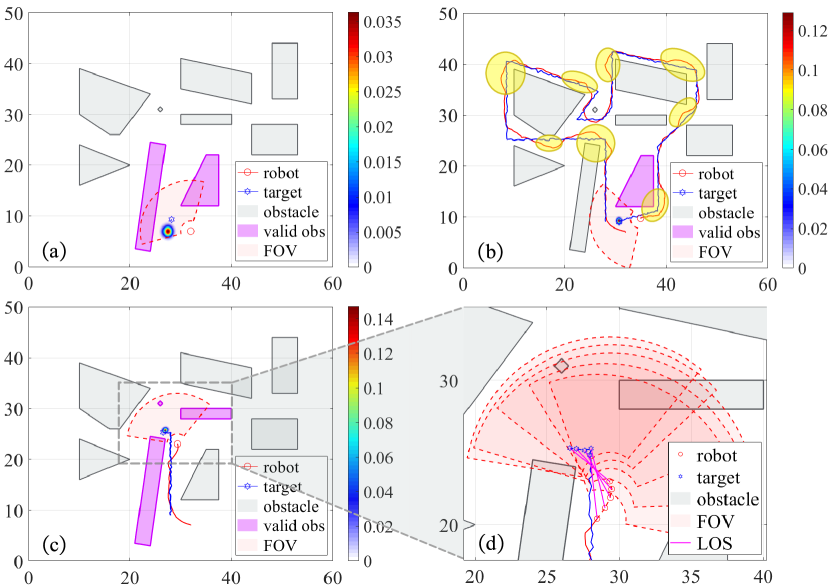
Figure 5: Visibility-aware tracking of the target with linear motion model. The colorful background represents the target’s PDF, and the color bar shows the colormap of probability. The “valid obs” denotes the valid obstacles. (a) Initial simulation scenario. (b) Entire tracking trajectory. (c) and (d) highlight a sharp turn of the target and display the robot’s trajectory with high visibility.

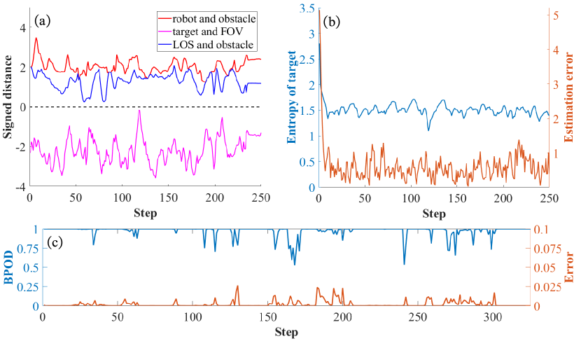
Figure 6: Trajectory performance. (a) History of signed distances. (b) Target entropy and estimation error. (c) The BPOD value and the approximation error of the BPOD compared to the ground truth.

Fig. 5 shows the tracking process. The target uncertainty is initialized to be very large (Fig. 5(a)). As the tracking progresses, the robot plans a visibility-aware trajectory to track the target (Fig. 5(b)). Specifically, when the target takes a sharp turn near an obstacle, the robot moves away from the obstacle in advance to reduce the likelihood of target loss (Fig. 5(c) and (d)). Note that this roundabout path frequently appears in the tracking process (highlighted by yellow ellipses in Fig. 5(b)) and is a characteristic of visibility-aware trajectories.

Fig. 6 displays the performance data. The robot can maintain the visibility of the target throughout the simulation without any target loss. To see this, Fig. 6(a) shows the purple curve that indicates the target is inside our convexified FOV most of the time, and the blue curve that indicates LOS and obstacles never intersect. Due to uninterrupted measurements, target entropy rapidly converges and the estimation error is kept small (Fig. 6(b)). We also record the BPOD value and evaluate the accuracy of the BPOD approximation against the Monte-Carlo simulation as the ground truth, as shown in Fig. 6(c). The subfigure shows that the BPOD is kept near $1$ most of the time although we don’t use the BPOD as the objective function directly, which verifies the compatibility of the two objectives Eq. 14. Results also demonstrate that we can calculate one BPOD within $1ms$ with an MAE of $2.5\times 10^{-3}$.

This experiment is conducted 50 times to verify the robustness of our method under measurement noise and imperfect control. The results show that the robot can track the target with low mean estimation error $\bar{e}_{est}=0.336m$, high mean visible rate $\bar{r}_{vis}=96.5$% and high success rate $r_{suc}=96$% with the mean computing time $\bar{t}_{cal}=0.23s/step$.

V-B Case 2: Target with Nonlinear Motion Model

The target takes a unicycle model[26] with the target state represented as $\mathbf{z}^{t}_{k}=[{\mathbf{x}^{t}_{k}}^{T},\theta^{t}_{k}]^{T}$, where $\theta^{t}_{k}$ stands for target orientation. In addition, the target controls $\mathbf{u}^{t}_{k}=[v^{t}_{k},\omega^{t}_{k}]^{T}$ that encode the speed $v^{t}_{k}\in\mathbb{R}$ and angular velocity $\omega^{t}_{k}\in\mathbb{R}$ remain unknown to the robot. Therefore, the robot estimates $\mathbf{u}^{t}_{k}$ by differentiating target displacement and rotation. We should note that this coarse control estimation poses a great challenge for the tracking task. We choose the cumulated BPOD $J_{2}$ in Eq. 14 as the objective function. We adopt a camera sensor model to detect target distance, bearing angle and orientation:

$$\mathbf{f}^{s}_{cam}(\mathbf{z}_{k}^{t},\mathbf{z}_{k}^{r})=[\|\mathbf{x}_{k}^{t}-\mathbf{x}_{k}^{r}\|,\angle(\mathbf{x}_{k}^{t}-\mathbf{x}_{k}^{r})-\theta^{r}_{k},\theta^{t}_{k}-\theta^{r}_{k}]^{T},$$

and the measurement noise is set as $10^{-2}\cdot diag(1,0.5,1)$.

To verify the generality of our algorithm, we set different target speed limits $v_{max}^{t}$ and implement the MATLAB Navigation Toolbox to randomly generate 50 trajectories with $400$ steps for each trajectory under each $v_{max}^{t}$. Target motion noise is set as $0.5\mathbf{I}_{3}$ to simulate stochastic target movements.

Examples of tracking experiments are presented in Fig. 7 and simulation results are shown in Tab. I. Results demonstrate that the proposed planner consistently maintains high visibility and success rates in tracking a target with highly-stochastic trajectories, achieving a computing speed of around $10Hz$. The increased computational time and decreased visible rate in the linear case result from the fact that the robot has to track a target with a highly challenging target trajectory, as illustrated in Fig. 5(b).

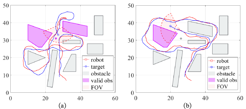
Figure 7: Two tracking simulations of the nonlinear target with randomly-generated trajectories.

TABLE I: Simulation Results for Case 2

$v_{max}^{t}$(m/s)	1	2	3
$\bar{t}_{cal}$(s/step)	0.114 $\pm$ 0.005	0.105 $\pm$ 0.005	0.092 $\pm$ 0.005
$\bar{e}_{est}$(m)	0.249 $\pm$ 0.007	0.261 $\pm$ 0.009	0.276 $\pm$ 0.011
$\bar{r}_{vis}$(%)	99.7 $\pm$ 0.4	99.7 $\pm$ 0.6	99.3 $\pm$ 0.9
$r_{suc}$(%)	100	100	96

VI Real-World Experiments

The proposed approach has been tested by using a Wheeltec ground robot equipped with an ORBBEC Femto W camera to keep track of a moving Turtlebot3, on which three interlinked Apriltags [27] are affixed. The speed limit of the tracker and the target are $0.4m/s$ and $0.31m/s$, respectively. The onboard processor (NVIDIA Jetson TX1) on the Wheeltec robot calculates the distance, bearing angle, and orientation of the detected Apriltag from the camera images and transmits the messages through ROS to a laptop (11th Intel(R) i7 CPU@2.30GHz) that performs the planning algorithm. The parameters of the sensor model are calibrated as $r_{1}=0.3m$, $r_{2}=1.5m$, $\theta=100^{\circ}$, and $\mathbf{R}^{s}=diag(0.069,8.3\times 10^{-4},0.0055)$. The covariance of robot motion noise is set as $\mathbf{R}^{r}=diag(0.08\mathbf{I}_{2},0.055\mathbf{I}_{2})$ to handle model discretization error and mechanical error. Other parameters are kept the same as Sec. V-B. The ground truth of the robot and target poses are obtained by a Vicon motion-capture system.

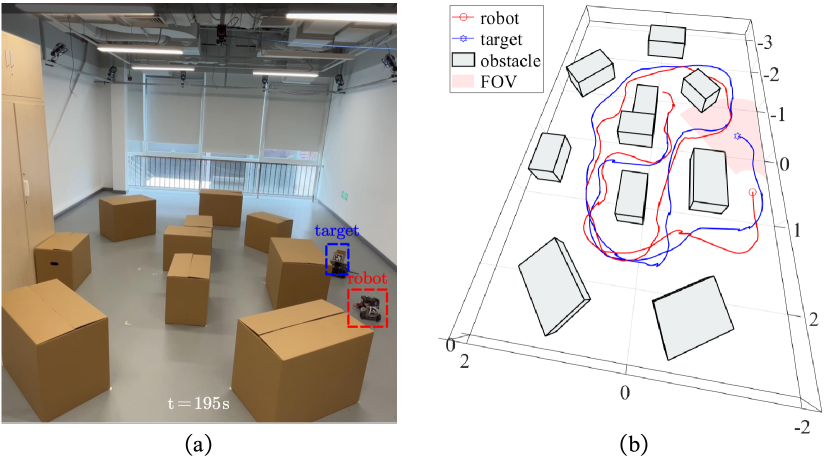
Figure 8: Real-world target tracking. (a) Map configuration and one tracking frame. (b) Simulation scene corresponding to (a) and the trajectories of the target and the robot.

We conduct three tracking experiments by remotely controlling the target to randomly traverse an indoor map with cluttered obstacles (Fig. 8(a)), and the duration of all three experiments exceed 2 minutes. For each experiment, we record the total planning steps $T$, estimation error $e_{est}$, calculation time $t_{cal}$ and minimum distance to obstacles $d_{min}$, as shown in Tab. II. Both Fig. 8(b) and Tab. II show that our planner can generate safe trajectories for the robot to track a moving target while reducing target uncertainty in real-world scenarios.

TABLE II: Real-World Experiment Results

	$T$	$e_{est}$(m)	$t_{cal}$(s/step)	$d_{min}$(m)
1	538	0.072	0.087	0.247
2	497	0.078	0.089	0.210
3	471	0.071	0.090	0.232

VII Conclusion

We propose a target-tracking approach that systematically accounts for the limited FOV, obstacle occlusion, and state uncertainty. In particular, the concept of BPOD is proposed and incorporated into the EKF framework to predict target uncertainty in systems subject to measurement noise and imperfect motion models. We subsequently develop an SDF-based method to efficiently calculate the BPOD and collision risk to solve the trajectory optimization problem in real time. Both simulations and real-world experiments validate the effectiveness and efficiency of our approach. Future work includes mainly two aspects. First, we will investigate the properties and applications of BPOD in non-Gaussian belief space planning. Second, we will extend the proposed method to unknown and dynamic environments.

Acknowledgement

We thank Dr. Meng Wang at BIGAI for his help with photography.

References

- [1] G. Punyavathi, M. Neeladri, and M. K. Singh, “Vehicle tracking and detection techniques using iot,” Materials Today: Proceedings, vol. 51, pp. 909–913, 2022.
- [2] X. Xu, G. Shi, P. Tokekar, and Y. Diaz-Mercado, “Interactive multi-robot aerial cinematography through hemispherical manifold coverage,” in Proceedings of International Conference on Intelligent Robots and Systems (IROS), IEEE, 2022.
- [3] M. Xanthidis, M. Kalaitzakis, N. Karapetyan, J. Johnson, N. Vitzilaios, J. M. O’Kane, and I. Rekleitis, “Aquavis: A perception-aware autonomous navigation framework for underwater vehicles,” in Proceedings of International Conference on Intelligent Robots and Systems (IROS), IEEE, 2021.
- [4] Y. Su, Y. Jiang, Y. Zhu, and H. Liu, “Object gathering with a tethered robot duo,” IEEE Robotics and Automation Letters (RA-L), vol. 7, no. 2, pp. 2132–2139, 2022.
- [5] C. Liu and J. K. Hedrick, “Model predictive control-based target search and tracking using autonomous mobile robot with limited sensing domain,” in American Control Conference (ACC), IEEE, 2017.
- [6] T. Li, L. W. Krakow, and S. Gopalswamy, “Sma-nbo: A sequential multi-agent planning with nominal belief-state optimization in target tracking,” in Proceedings of International Conference on Intelligent Robots and Systems (IROS), IEEE, 2022.
- [7] Q. Wang, Y. Gao, J. Ji, C. Xu, and F. Gao, “Visibility-aware trajectory optimization with application to aerial tracking,” in Proceedings of International Conference on Intelligent Robots and Systems (IROS), IEEE, 2021.
- [8] J. Ji, N. Pan, C. Xu, and F. Gao, “Elastic tracker: A spatio-temporal trajectory planner for flexible aerial tracking,” in Proceedings of International Conference on Robotics and Automation (ICRA), IEEE, 2022.
- [9] D. Falanga, P. Foehn, P. Lu, and D. Scaramuzza, “Pampc: Perception-aware model predictive control for quadrotors,” in Proceedings of International Conference on Intelligent Robots and Systems (IROS), IEEE, 2018.
- [10] B. Penin, P. R. Giordano, and F. Chaumette, “Vision-based reactive planning for aggressive target tracking while avoiding collisions and occlusions,” IEEE Robotics and Automation Letters (RA-L), vol. 3, no. 4, pp. 3725–3732, 2018.
- [11] H. Masnavi, J. Shrestha, M. Mishra, P. Sujit, K. Kruusamäe, and A. K. Singh, “Visibility-aware navigation with batch projection augmented cross-entropy method over a learned occlusion cost,” IEEE Robotics and Automation Letters (RA-L), vol. 7, no. 4, pp. 9366–9373, 2022.
- [12] B. Jeon, Y. Lee, and H. J. Kim, “Integrated motion planner for real-time aerial videography with a drone in a dense environment,” in Proceedings of International Conference on Robotics and Automation (ICRA), IEEE, 2020.
- [13] S. Patil, Y. Duan, J. Schulman, K. Goldberg, and P. Abbeel, “Gaussian belief space planning with discontinuities in sensing domains,” in Proceedings of International Conference on Robotics and Automation (ICRA), IEEE, 2014.
- [14] H. Yu, K. Meier, M. Argyle, and R. W. Beard, “Cooperative path planning for target tracking in urban environments using unmanned air and ground vehicles,” IEEE/ASME Transactions on Mechatronics (TMECH), vol. 20, no. 2, pp. 541–552, 2014.
- [15] C. Zhang and I. Hwang, “Multiple maneuvering target tracking using a single unmanned aerial vehicle,” Journal of guidance, control, and dynamics, vol. 42, no. 1, pp. 78–90, 2019.
- [16] B. Sinopoli, L. Schenato, M. Franceschetti, K. Poolla, M. I. Jordan, and S. S. Sastry, “Kalman filtering with intermittent observations,” IEEE transactions on Automatic Control, vol. 49, no. 9, pp. 1453–1464, 2004.
- [17] S. Papaioannou, P. Kolios, T. Theocharides, C. G. Panayiotou, and M. M. Polycarpou, “Jointly-optimized searching and tracking with random finite sets,” IEEE Transactions on Mobile Computing, vol. 19, no. 10, pp. 2374–2391, 2020.
- [18] S. Haykin, Kalman filtering and neural networks. John Wiley & Sons, 2004.
- [19] M. Marcus and H. Minc, A survey of matrix theory and matrix inequalities, vol. 14. Courier Corporation, 1992.
- [20] T. M. Cover, Elements of information theory. John Wiley & Sons, 1999.
- [21] L. Blackmore, M. Ono, and B. C. Williams, “Chance-constrained optimal path planning with obstacles,” IEEE Transactions on Robotics (T-RO), vol. 27, no. 6, pp. 1080–1094, 2011.
- [22] J. Schulman, Y. Duan, J. Ho, A. Lee, I. Awwal, H. Bradlow, J. Pan, S. Patil, K. Goldberg, and P. Abbeel, “Motion planning with sequential convex optimization and convex collision checking,” International Journal of Robotics Research (IJRR), vol. 33, no. 9, pp. 1251–1270, 2014.
- [23] E. G. Gilbert, D. W. Johnson, and S. S. Keerthi, “A fast procedure for computing the distance between complex objects in three-dimensional space,” IEEE Journal on Robotics and Automation, vol. 4, no. 2, pp. 193–203, 1988.
- [24] G. Van Den Bergen, “Proximity queries and penetration depth computation on 3d game objects,” in Game developers conference, vol. 170, 2001.
- [25] A. Prékopa, Stochastic programming, vol. 324. Springer Science & Business Media, 2013.
- [26] S. M. LaValle, Planning algorithms. Cambridge university press, 2006.
- [27] E. Olson, “Apriltag: A robust and flexible visual fiducial system,” in Proceedings of International Conference on Robotics and Automation (ICRA), IEEE, 2011.